PINF: Continuous Normalizing Flows for Physics-Constrained Deep Learning
Abstract
The normalization constraint on probability density poses a significant challenge for solving the Fokker-Planck equation. Normalizing Flow, an invertible generative model leverages the change of variables formula to ensure probability density conservation and enable the learning of complex data distributions. In this paper, we introduce Physics-Informed Normalizing Flows (PINF), a novel extension of continuous normalizing flows, incorporating diffusion through the method of characteristics. Our method, which is mesh-free and causality-free, can efficiently solve high dimensional time-dependent and steady-state Fokker-Planck equations.
1 Introduction
The Fokker-Planck (FP) equation (Risken, 1996) is a well-known partial differential equation that describes the evolution of a stochastic system’s probability density function (PDF) over time. Due to the high-dimensional variable and unbounded domain, traditional numerical methods, such as the finite difference methods (FDM) (Kumar & Narayanan, 2006), the finite element methods (FEM) (Deng, 2009), and the path integral methods (Wehner & Wolfer, 1983) prove to be computationally daunting in tackling the FP equations. By contrast, deep learning algorithms (Sirignano & Spiliopoulos, 2018; Raissi et al., 2019; Weinan & Yu, 2018), without a specific network structure, violate the normalization constraint on PDF, resulting in reduced accuracy and prevalent errors.
Recently, researchers have recognized the potential of flow-based generative models in learning complicated probability distributions (Kingma & Dhariwal, 2018; Ho et al., 2019; Albergo et al., 2019), alongside the connection to optimal transport (OT) theory (Finlay et al., 2020; Yang & Karniadakis, 2020; Zhang et al., 2018). Tang et al. (2022) employed normalizing flows as alternative solutions and proposed the KRnet for solving the steady-state Fokker-Planck (SFP) equations. However, the discrete normalizing flow remains circumscribed to model a single target distribution at a time, typically the final or steady-state distribution, thus constraining its utility in the time-dependent Fokker-Planck (TFP) equations. Consequently, Feng et al. (2022) introduced the temporal normalizing flow (TNF) to estimate time-dependent distributions for TFP equations, albeit without encapsulating the inherent physical laws of FP equations in structure.
More naturally, we generalize the continuous normalizing flow (CNF) (Chen et al., 2018) with diffusion and propose a novel intelligent architecture: Physics-Informed Normalizing Flows (PINF) for solving FP equations. We encode the physical constraints into ordinary differential equations (ODEs) using the method of characteristics and train the model in a self-supervised way. Numerical experiments demonstrate both accuracy and efficiency in solving high-dimensional TFP and SFP equations, even without the need for meticulous hyperparameter tuning.
2 Problem definition
Here we first give a brief introduction to the FP equation. Consider the state variable described by the stochastic differential equation (SDE) (Oksendal, 2013):
| (1) |
where the drift coefficient is a vector field, is a matrix-valued function and is an -dimensional standard Wiener process. The probability density function of satisfies the following Fokker-Planck equation:
| (2) | ||||
where denote the spatial-temporal variables, is the diffusion matrix, is the initial PDF of , is defined with the unbounded boundary condition, is an operator for spatial variables and indicates the norm of .
The stationary solution of Eq.(2) means the invariant measure independent of time, satisfying
| (3) |
More specifically, i.e.,
| (4) |
For the physical background of the FP equation, there are some extra constraints on its solution :
| (5) | ||||
which are called normalization and nonnegativity constraints.
3 Related work
To better describe our algorithm and its connections with flow-based models, it is worthwhile to review prior research on normalizing flows.
3.1 Normalizing flows and change of variables
Given a latent variable drawn from a simple prior probability distribution . When normalizing flows transform into using a bijection , the probability density function of follows the change of variables formula:
| (6) |
where is the Jacobian of at .
To describe a complex target distribution, a sequence of invertible and learnable mappings represented as are constructed and denotes the trainable parameter of the neural network. Let , then the density of is computed by
| (7) |
There are some simple optional structures, such as planar flows and radial flows (Rezende & Mohamed, 2015). A key challenge is to increase the representative power of normalizing flows while simplifying the computation of the associated Jacobian determinant. NICE (Dinh et al., 2015) employed affine coupling layers, duplicating a portion of the input while transforming the remaining part, thereby maintaining reversibility. Real NVP (Dinh et al., 2016) introduced scale and translation parameters, further improving the performance of the flow. Additionally, the Jacobian of Real NVP transformations has a specific lower triangular structure, ensuring efficient computations with linear time complexity for the logdet-Jacobian term.
It is important to note that the resulting target distribution adheres to the probability normalization constraint, as guaranteed by the change of variables formula.
| (8) |
3.2 Continuous normalizing flows and instantaneous change of variables
Chen et al. (2018) proposed the Neural ODE framework and derived the finite normalizing flows to a continuous limit scheme, effectively expressing the invertible mappings using ODEs. The latent variable and its log probability change according to the instantaneous change of variables theorem (Villani, 2003):
| (9) |
By leveraging the adjoint sensitivity method to resolve augmented ODEs in reverse time, CNF computes gradients with respect to and is trained directly using maximum likelihood. An unexpected side-benefit is that the likelihood can be calculated using relatively cheap trace operations instead of the Jacobian determinant. Moreover, the entire transformation is automatically bijective when Eq.(9) has a unique solution. Therefore, the mapping does not need to be bijective.
3.3 Relationship between continuous normalizing flows and Fokker-Planck equations
Continuous normalizing flows can be related to the special case of the FP equation with zero diffusion, known as the Liouville equation. Let evolve through time according to the degenerate Eq.(1): . As shown in Eq.(2), the probability density function satisfies the FP equation represented as:
| (10) |
To compute the value of , the characteristics method tracks the trajectory of a particle . The total derivative of is given by
| (11) |
By dividing on both sides, we obtain the same result as Eq.(9). (See Appendix A.2 in Chen et al. (2018) for more details).
4 PINF: Physics-Informed Normalizing Flows
Let us begin by introducing the PINF algorithm for time-dependent FP equations, categorizing them into two scenarios based on whether the diffusion term is zero. Subsequently, we will present the special design of the algorithm for solving the steady-state FP equation.
4.1 Time-dependent Fokker-Planck equations
The TFP equation is essentially an initial value problem (2), where the initial density function is known.
4.1.1 TFP equation with zero diffusion
Problem Setup:
| (12) | ||||
The objective of solving the TFP equation is to compute the density at any given point . Following the derivation in Eq.(11), the TFP equation can be reformulated as an initial value problem of ODEs.
| (13) |
Notably, the increment in is independent of its value and solely depends on the start time , the stop time , and the value of . Therefore, the initial states for can be set as , and the solution is obtained by using the corresponding output of ODE solvers, yielding . The specific algorithm is outlined as follows:
The key distinction between PINF and CNF lies in the fact that the drift is known in the TFP equation. In this context, there is no need to train from the real data samples and we can simply use ODE solvers once to obtain the outcomes.
4.1.2 TFP equation with diffusion
Problem Setup:
| (14) | ||||
We first perform some necessary transformations of the equation.
| (15) | ||||
Let us define . We force to evolve through time following and get the associated ODEs by Eq.(11).
| (16) |
In particular, unlike the zero diffusion case, the ODE dynamics depend on the unknown function and its gradient will not be evaluated during the forward calculation. For this reason, we parameterize as a neural network .
Neural network architecture. The network structure is inspired by the value function representations used for stochastic optimal control (Li et al., 2022), multi-agent optimal control (Onken et al., 2021b), and high-dimensional optimal control (Onken et al., 2022). The network is given by
| (17) |
where are the trainable weights of . The shapes of those parameters are listed as follows: the inputs corresponding to space–time, , , , , and . The rank is set to limit the number of parameters in . Here, , , and model quadratic potentials, i.e., linear dynamics; models nonlinear dynamics.
In our implementation, for , we use a residual neural network (ResNet) (He et al., 2016) with layers and obtain as the final step of the forward propagation
| (18) | ||||
where the trainable weights are , and . We select the step size and the element-wise activation function (Onken et al., 2021a), which is the antiderivative of the hyperbolic tangent, i.e., . It can also be seen as a smoothed absolute value function (Ruthotto et al., 2020).
To satisfy the initial value condition , the network is cast as
| (19) |
to represent (Lagaris et al., 1998). This structured design can impose hard constraints that are strictly enforced, rather than soft constraints (Wang & Yu, 2021).
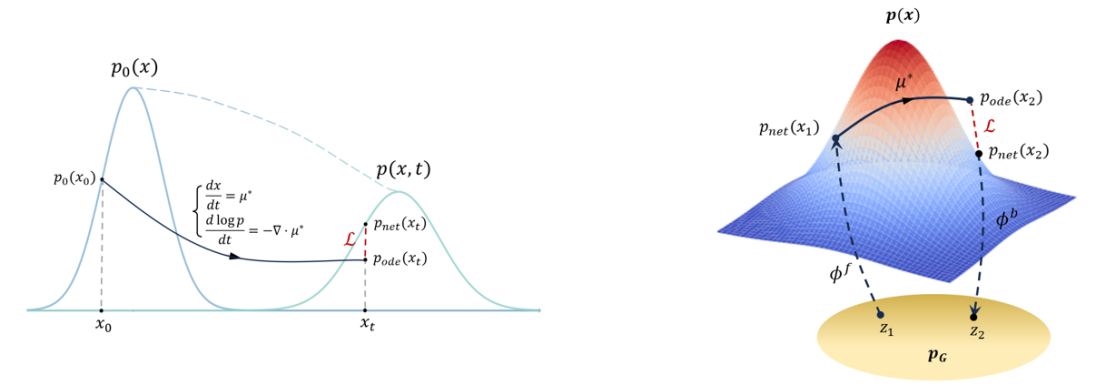
Self-supervised training method. Distinct from normalizing flows that minimize the Kullback-Leibler divergence, we employ a self-supervised training method. Our approach eliminates the need for labeled data or real data samples from the target distribution, which are sometimes challenging or costly to acquire. Training data is adaptively generated based on the initial PDF.
For training , we solve the ODEs (16) related to the network , obtaining predictions in the form of . Moreover, the network can also output the prediction directly. We calculate the Mean Squared Error (MSE) between and and use the Adam optimizer (Kingma & Ba, 2014).
| (20) |
To address issues such as small gradients and optimization difficulties in high-dimensional scenarios, we avoid comparing directly in the loss function: . Experimental results also demonstrate that applying the logarithm function accelerates the training process.
Flexible prediction modes. With the trained , we provide two flexible prediction modes: numerical solutions solved by ODE solvers and continuous solutions predicted by neural networks. This flexibility enables a trade-off between efficiency and accuracy, maintaining advantages such as memory efficiency, adaptive solvers, and parallel computation (Kang et al., 2021). When using neural networks for prediction, our approach is mesh-free and causality-free (Nakamura-Zimmerer et al., 2020), similar to PINNs. Data at different time steps can be computed rapidly and in parallel, allowing for real-time or low-power applications. Alternatively, when using ODE solvers for prediction, we can freely choose from modern ODE solvers for adaptive computation (Runge, 1895; Wanner & Hairer, 1996). See Alg.(2) for the complete algorithm.
4.2 Steady-state Fokker-Planck equations
Problem Setup:
| (21) | ||||
The SFP equation replaces the initial value condition with an equation constraint (3), ensuring that its solution remains invariant over time. Therefore, the steady-state PDF only depends on spatial variables and we derive another form of our problem:
| (22) |
Normalization Challenge. In the TFP equations, since the initial PDF satisfies the normalization constraint, the total density integral on the space domain remains conserved as the solution evolves under equation constraints or ODEs controls. Consequently, the solution predicted by the PINF algorithm also satisfies the normalization constraint.
However, for the SFP equations, it is easily checked that if is the solution, then any ( is a constant) also satisfies the equation. In the ODEs, the scheme remains unchanged due to . Hence, starting from and evolving through to , both ODEs associated with and reach the same point and have the same increment . For the ODEs of , the predicted value of is given by
| (23) | ||||
Ultimately, and satisfy the ODEs.
Neural network architecture. We still employ a neural network to parameterize in ODEs (16). For the normalization constraint, we adopt the Real NVP (Dinh et al., 2016) to model the equilibrium distribution from a Gaussian distribution . We stack affine coupling layers to build a flexible and tractable bijective transformation. At each layer, given the input and dimension , the output is defined as
| (24) | ||||
where and represent scale and translation, and is the element-wise product. The Jacobian of this transformation is triangular, reads
| (25) |
Consequently, we can efficiently compute its log-determinant as .
Since partitioning can be implemented using a binary mask , the forward and backward computation processes respectively follow the equations,
| Forward: | (26) | |||
| Backward: | ||||
Here, are constructed via a simple 3-layer MLP (Goodfellow et al., 2016) with the activation function .
| (27) | ||||
The self-supervised training method and loss function remain consistent with the previous description. This is the PINF algorithm for SFP equations.
5 Experiment
In this section, we consider the following three numerical examples to test the performance of our PINF algorithm.
5.1 A toy example
We first present a toy example, a TFP equation with zero diffusion. We employ it to illustrate that our PINF algorithm is the method of characteristics in mathematics.
| (28) | ||||
Here denotes an all-ones vector, and the diffusion term is independent of . The corresponding ODEs obtained through the PINF algorithm (1) are as follows:
| (29) |
Consequently, the analytical solution of the equation is
| (30) |
5.2 TFP equation
We consider a relatively high-dimensional TFP equation. For this problem, the PINN is effective primarily with the dimension .
| (31) | ||||
The exact solution is given by
| (32) |
Using the PINF algorithm (2), we formulate the ODEs as
| (33) |
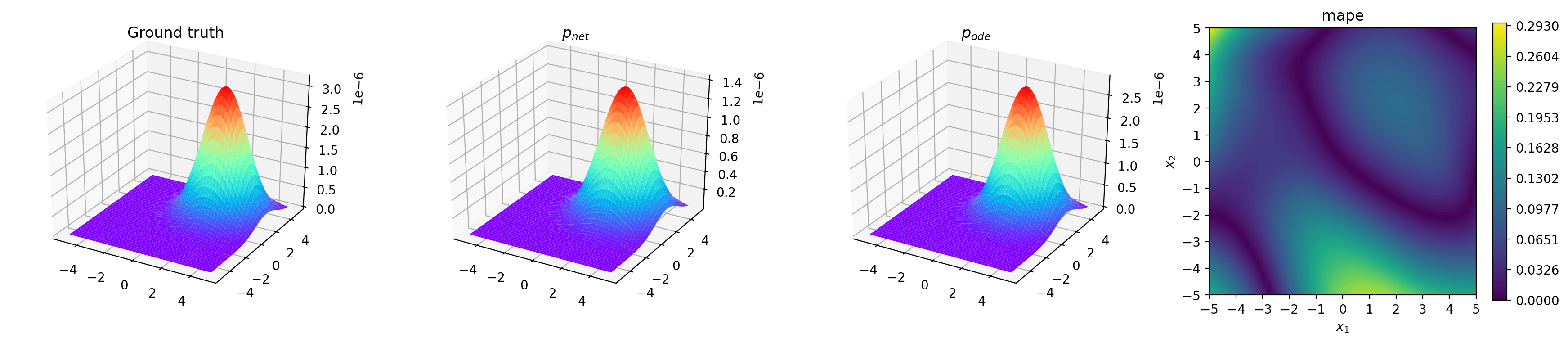
We solve this TFP equation of . We take residual layers with hidden neurons and set training iteration , the learning rate for Adam optimizer , and the batch size is . The initial spatial training set is generated from , and the corresponding temporal training set is uniformly sampled in the interval . We evaluate the performance of our PINF algorithm at the point and the stop time , where is drawn from a uniform grid within the finite spatial domain . The comparison between the prediction and the ground truth is shown in Fig.(2) and we observe a good agreement.
5.3 High dimensional SFP equation
In this part, a SFP equation with drift term and diffusion matrix is considered.
| (34) |
Its exact solution is a single Gaussian distribution, represented as
| (35) |
In our experiment, we set and evaluate our PINF algorithm on the SFP equation with dimensions and . We employ affine coupling layers and set , , batch size is . Since its steady-state solution is an unimodal function near the origin, we select the test points as , where is drawn from a uniform grid within the range , resulting in total test points. Fig.(3) shows the exact solution and our PINF solution , where it can be seen that they are visually indistinguishable, and the relative error remains below 0.2%, even for relatively high dimensions.
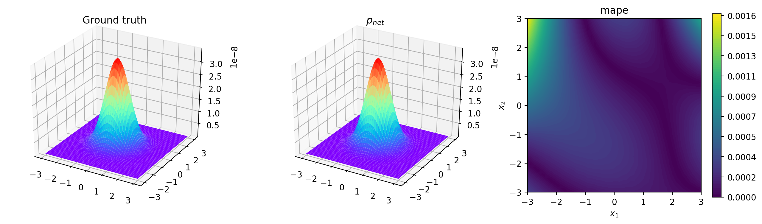

Bottom row: d=50.
6 Discussion
Our proposed PINF algorithm extends CNF to the scheme with diffusion using the method of characteristics. Compared to PINNs, which apply pointwise equation constraints, our improvements are mainly in reformulating the FP equation as ODEs and computing the integral of the loss along characteristic curves using an ODE solver, thereby enhancing training efficiency and stability. It effectively addresses the normalization constraint of the PDF even in high-dimensional FP problems.
The critical distinction between PINF for FP equations and CNF for density estimation lies in whether the drift term is known. In FP equations, the drift term is known and we obtain its solution by self-supervised training of a neural network. Conversely, the drift term necessitates likelihood-based training for the latter. In future work, we may explore the application of PINF with diffusion for density estimation tasks to enhance model generalization and data generation quality.
Considering the profound physical significance and wide-ranging applications of FP equations, the PINF algorithm can also be seamlessly integrated with large-scale mean-field games for optimal control problems, such as path planning, obstacle avoidance, and tracking in drone swarm applications.
References
- Albergo et al. (2019) Michael S Albergo, Gurtej Kanwar, and Phiala E Shanahan. Flow-based generative models for markov chain monte carlo in lattice field theory. Physical Review D, 100(3):034515, 2019.
- Chen et al. (2018) Ricky TQ Chen, Yulia Rubanova, Jesse Bettencourt, and David K Duvenaud. Neural ordinary differential equations. Advances in neural information processing systems, 31, 2018.
- Deng (2009) Weihua Deng. Finite element method for the space and time fractional fokker–planck equation. SIAM journal on numerical analysis, 47(1):204–226, 2009.
- Dinh et al. (2015) L Dinh, D Krueger, and Y Bengio. Nice: non-linear independent components estimation. In International Conference on Learning Representations Workshop, 2015.
- Dinh et al. (2016) Laurent Dinh, Jascha Sohl-Dickstein, and Samy Bengio. Density estimation using real nvp. In International Conference on Learning Representations, 2016.
- Feng et al. (2022) Xiaodong Feng, Li Zeng, and Tao Zhou. Solving time dependent fokker-planck equations via temporal normalizing flow. Communications in Computational Physics, 32(2):401–423, 2022.
- Finlay et al. (2020) Chris Finlay, Jörn-Henrik Jacobsen, Levon Nurbekyan, and Adam Oberman. How to train your neural ode: the world of jacobian and kinetic regularization. In International conference on machine learning, pp. 3154–3164. PMLR, 2020.
- Goodfellow et al. (2016) Ian Goodfellow, Yoshua Bengio, and Aaron Courville. Deep learning. MIT press, 2016.
- He et al. (2016) Kaiming He, Xiangyu Zhang, Shaoqing Ren, and Jian Sun. Deep residual learning for image recognition. In Proceedings of the IEEE conference on computer vision and pattern recognition, pp. 770–778, 2016.
- Ho et al. (2019) Jonathan Ho, Xi Chen, Aravind Srinivas, Yan Duan, and Pieter Abbeel. Flow++: Improving flow-based generative models with variational dequantization and architecture design. In International Conference on Machine Learning, pp. 2722–2730. PMLR, 2019.
- Kang et al. (2021) Wei Kang, Qi Gong, Tenavi Nakamura-Zimmerer, and Fariba Fahroo. Algorithms of data generation for deep learning and feedback design: A survey. Physica D: Nonlinear Phenomena, 425:132955, 2021.
- Kingma & Ba (2014) Diederik P Kingma and Jimmy Ba. Adam: A method for stochastic optimization. arXiv preprint arXiv:1412.6980, 2014.
- Kingma & Dhariwal (2018) Durk P Kingma and Prafulla Dhariwal. Glow: Generative flow with invertible 1x1 convolutions. Advances in neural information processing systems, 31, 2018.
- Kumar & Narayanan (2006) Pankaj Kumar and S Narayanan. Solution of fokker-planck equation by finite element and finite difference methods for nonlinear systems. Sadhana, 31:445–461, 2006.
- Lagaris et al. (1998) Isaac E Lagaris, Aristidis Likas, and Dimitrios I Fotiadis. Artificial neural networks for solving ordinary and partial differential equations. IEEE transactions on neural networks, 9(5):987–1000, 1998.
- Li et al. (2022) Xingjian Li, Deepanshu Verma, and Lars Ruthotto. A neural network approach for stochastic optimal control. arXiv preprint arXiv:2209.13104, 2022.
- Nakamura-Zimmerer et al. (2020) Tenavi Nakamura-Zimmerer, Qi Gong, and Wei Kang. A causality-free neural network method for high-dimensional hamilton-jacobi-bellman equations. In 2020 American Control Conference (ACC), pp. 787–793. IEEE, 2020.
- Oksendal (2013) Bernt Oksendal. Stochastic differential equations: an introduction with applications. Springer Science & Business Media, 2013.
- Onken et al. (2021a) Derek Onken, Samy Wu Fung, Xingjian Li, and Lars Ruthotto. Ot-flow: Fast and accurate continuous normalizing flows via optimal transport. Proceedings of the AAAI Conference on Artificial Intelligence, 35(10):9223–9232, 2021a.
- Onken et al. (2021b) Derek Onken, Levon Nurbekyan, Xingjian Li, Samy Wu Fung, Stanley Osher, and Lars Ruthotto. A neural network approach applied to multi-agent optimal control. In 2021 European Control Conference (ECC), pp. 1036–1041. IEEE, 2021b.
- Onken et al. (2022) Derek Onken, Levon Nurbekyan, Xingjian Li, Samy Wu Fung, Stanley Osher, and Lars Ruthotto. A neural network approach for high-dimensional optimal control applied to multi-agent path finding. IEEE Transactions on Control Systems Technology, 31(1):235–251, 2022.
- Raissi et al. (2019) Maziar Raissi, Paris Perdikaris, and George E Karniadakis. Physics-informed neural networks: A deep learning framework for solving forward and inverse problems involving nonlinear partial differential equations. Journal of Computational Physics, 378:686–707, 2019.
- Rezende & Mohamed (2015) Danilo Rezende and Shakir Mohamed. Variational inference with normalizing flows. In International conference on machine learning, pp. 1530–1538. PMLR, 2015.
- Risken (1996) Hannes Risken. Fokker-planck equation. Springer, 1996.
- Runge (1895) Carl Runge. Über die numerische auflösung von differentialgleichungen. Mathematische Annalen, 46(2):167–178, 1895.
- Ruthotto et al. (2020) Lars Ruthotto, Stanley J Osher, Wuchen Li, Levon Nurbekyan, and Samy Wu Fung. A machine learning framework for solving high-dimensional mean field game and mean field control problems. Proceedings of the National Academy of Sciences, 117(17):9183–9193, 2020.
- Sirignano & Spiliopoulos (2018) Justin Sirignano and Konstantinos Spiliopoulos. Dgm: A deep learning algorithm for solving partial differential equations. Journal of computational physics, 375:1339–1364, 2018.
- Tang et al. (2022) Kejun Tang, Xiaoliang Wan, and Qifeng Liao. Adaptive deep density approximation for fokker-planck equations. Journal of Computational Physics, 457:111080, 2022.
- Villani (2003) Cédric Villani. Topics in Optimal Transportation. Number 58. American Mathematical Soc., 2003.
- Wang & Yu (2021) Rui Wang and Rose Yu. Physics-guided deep learning for dynamical systems: A survey. arXiv preprint arXiv:2107.01272, 2021.
- Wanner & Hairer (1996) Gerhard Wanner and Ernst Hairer. Solving ordinary differential equations II, volume 375. Springer Berlin Heidelberg New York, 1996.
- Wehner & Wolfer (1983) M Fo Wehner and WG Wolfer. Numerical evaluation of path-integral solutions to fokker-planck equations. Physical Review A, 27(5):2663, 1983.
- Weinan & Yu (2018) E Weinan and Bing Yu. The deep ritz method: A deep learning-based numerical algorithm for solving variational problems. Communications in Mathematics and Statistics, 6(1):1–12, 2018.
- Yang & Karniadakis (2020) Liu Yang and George Em Karniadakis. Potential flow generator with optimal transport regularity for generative models. IEEE Transactions on Neural Networks and Learning Systems, 33(2):528–538, 2020.
- Zhang et al. (2018) Linfeng Zhang, Lei Wang, et al. Monge-ampère flow for generative modeling. arXiv e-prints, pp. arXiv–1809, 2018.