Quasilocal Corrections to Bondi’s Mass-Loss Formula and Dynamical Horizons
Abstract
In this work, a null geometric approach to the Brown-York quasilocal formalism is used to derive an integral law that describes the rate of change of mass and/or radiative energy escaping through a dynamical horizon of a non-stationary spacetime. The result thus obtained shows - in accordance with previous results from the theory of dynamical horizons of Ashtekar et al. - that the rate at which energy is transferred from the bulk to the boundary of spacetime through the dynamical horizon becomes zero at equilibrium, where said horizon becomes non-expanding and null. Moreover, it reveals previously unrecognized quasilocal corrections to the Bondi mass-loss formula arising from the combined variation of bulk and boundary components of the Brown-York Hamiltonian, given in terms of a bulk-to-boundary inflow term akin to an expression derived in an earlier paper by the author [17]. For clarity, this is discussed with reference to the Generalized Vaidya family of spacetimes, for which derived integral expressions take a particularly simple form.
Key words: quasilocal Hamiltonian, dynamical horizons, Bondi mass-loss formula
Introduction
To determine within the Brown-York quasilocal formalism [10, 13] the change in mass and/or radiant energy escaping through the spatial boundary of a finitely extended gravitating physical system, it generally incurs, as only recently shown in [17], the necessity to calculate the time derivative of the total quasilocal gravitational Hamiltonian (bulk plus boundary term) rather than just that of the boundary part. The main reason for this is that the temporal variation of the ADM Hamiltonian, which corresponds to the bulk part of the total expression mentioned above, yields a non-vanishing bulk-to-boundary inflow term that leads to corrections to Einstein’s quadrupole formula in the linearized weak-field approximation of general relativity.
This integral term, if different from zero (which is possible only in the non-vacuum case), has been shown to play a role in the quasilocal description of various physical phenomena, such as tidal deformation and heating processes as well as gravitoelectromagnetic effects [17]. Moreover, as has also been shown, its existence entails some remarkable consequences, perhaps the most striking of which is that the corrections it causes lead to a shift in the overall intensity of gravitational radiation emanating from compact gravitational sources such as stars and black holes. This is remarkable not least because the intensity shift in question should in principle prove to be experimentally detectable resp. observable in gravitational wave simulations, thus leading to a physical prediction that can readily be tested with modern methods of gravitational wave astronomy.
The main problem in this respect, however, is that it has not yet been clearly established whether the corrections caused by the mentioned inflow term are smaller or of the same order of magnitude as other integral terms resulting from the variation of the quasilocal Brown-York Hamiltonian. Moreover, with the exception of selected models of linearized Einstein-Hilbert gravity, the precise physical meaning of the corrections in question has remained elusive to this day.
In response to these shortcomings, the present work takes a specific approach to the subject by calculating within a bounded non-stationary spacetime the flux of mass and/or radiant energy through the dynamical horizon of the geometry, as well as its temporal variation. As a basis for these calculations, a null geometric approach to the quasilocal Brown-York formalism is pursued, which is shown to be compatible with the powerful dynamical horizon framework of Ashtekar et al. [6, 7] and Hayward’s related trapping horizon approach [16]. To this end, following a previous work on the subject [11], a geometric setting is introduced that involves a spatially and temporally bounded spacetime with inner and outer boundaries, where the inner boundary is given by a dynamical horizon. Regarding this particular geometric setting, the time-flow vector field of spacetime is then chosen to coincide once with the lightlike horizon vector field of the geometry (which is generally non-tangential to said horizon) and once with the same horizon vector field plus a boundary shift vector, and the resulting total Hamiltonian is varied with respect to these same vector fields. Thereby, it is shown that the methods used naturally lead to a null geometric equivalent of the bulk-to-boundary inflow term derived in [17] and thus to a corresponding intensity shift of emitted gravitational radiation.
The latter is concluded from the fact that the resulting quasilocal corrections do not vanish even if the outer boundary of spacetime is shifted to infinity in the large sphere limit. In lieu thereof, as shown in the second section of the paper, a modification of Bondi’s celebrated mass-loss formula [9, 18] results in such a case, which shows that radiative contributions at infinity can occur even if the Bondi news function is zero, and thus supposedly the time derivative of the associated mass aspect. It thus appears that, according to the quasilocal Hamiltonian formalism, there are exceptions to the generally accepted rule: The mass of a system is constant if and only if there is no news. As it seems, no similar result has been obtained in the literature so far. The quasilocal corrections responsible for this fact are determined explicitly in section two of the work.
For the standard choice for the lapse function proposed in the dynamical horizon framework, the result thus obtained shows that the temporal variation of the total quasilocal Brown-York Hamiltonian vanishes once the horizon reaches a steady state of equilibrium and becomes an isolated or weakly isolated horizon in the sense of [1, 2, 3, 4, 5]. Thus, in agreement with the common expectation, the discussed model confirms that any matter and/or radiation flux (of the specified type) from the bulk to the boundary of spacetime that crosses a dynamical horizon necessarily subsides completely in the limiting case where the local horizon geometry becomes stationary and settles into a state of equilibrium, as in the case of a black hole.
To eventually assess the magnitude of the integral terms involved and to provide an explicit example of non-vanishing radiative contributions at infinity, the corresponding expressions are calculated in the third and final section of the paper with respect to models of the Generalized Vaidya spacetime family, for which the resulting integral expressions take a particularly simple form in case that the boundary of spacetime is shifted to infinity in the large sphere limit. In doing so, it is shown that radiation fields may be detected at null infinity even in cases where the Bondi news function is zero, and that the resulting quasilocal corrections depend to a large extent on the choice of the time-flow vector field of the geometry. Potential implications of these findings are discussed towards the end of the paper.
1 Quasilocal Hamiltonian and Mass-Energy Transfer in Bounded Gravitational Fields
In this first preliminary section, the geometric setting to be considered is introduced, and some of the main results of [17] are recapitulated and generalized to fit this same setting. In particular, the time derivative of the quasilocal Brown-York gravitational Hamiltonian is calculated in a spacetime with interior and exterior boundaries, leading to an integral law describing how the matter and/or radiation content of a spatially and temporally bounded gravitating physical system changes with time. The bulk-to-boundary inflow term mentioned in the introduction is derived in the process, and it is shown what form some of the relevant integral expressions take with respect to the special choice of a lightlike (horizon) time-flow vector field of spacetime.
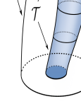
As a basis for the ensuing calculations, the present section essentially takes up the geometric setting considered in [17]. However, the latter is to be extended to comply with the dynamical horizon framework of Ashtekar et al. [6] in a manner similar to an earlier, slightly related work by Booth and Fairhurst [11]. For this purpose, let a fully dynamical, spatially compact, time orientable spacetime with manifold structure be considered, which is foliated by a family of -hypersurfaces . This spacetime may be envisioned as a non-stationary spacetime in a ’box’, i.e., a dynamical spacetime with a cylindrical outer boundary, the latter being later shifted to infinity. In more concrete terms, the boundary of said spacetime shall consist of two parts: an exterior part and an an interior part such that . The exterior part of the boundary shall be chosen in such a way that applies, where and represent spatial boundary parts, while represents a timelike boundary portion. This timelike portion shall be assumed to be foliated by a collection of two-surfaces such that . Additionally, it shall be assumed that there exists an interior boundary , where is a spacelike hypersurface representing a (canonical) dynamical horizon in the sense of Ashtekar et al. That is to say, is assumed to be a smooth, three-dimensional, spacelike submanifold of spacetime that exhibits a foliation by marginally trapped surfaces such that relative to each leaf of the foliation there exist two null normals and and two associated null expansion scalars and , where is the inverse of the induced metric , one of which vanishes locally and the other of which is strictly negative, i.e. and on .
Taking these assumptions as a starting point, the results of [17] shall be recapitulated in the following. To this end, the conventions of the mentioned work shall be adopted and adapted to the given geometric setting. To start with, a future-directed time evolution vector field shall be considered, which, at the timelike boundary , takes the form , where and are the corresponding lapse function and shift vector field as usual, is the normalized timelike generator leading to the the spacelike slicing of , is some timelike vector field tangent to and orthogonal to and and are the corresponding boundary lapse function and boundary shift vector field, respectively. Given this vector field and the related conventions, the corresponding three-metric at reads . To define the induced three-metric at , on the other hand, one may additionally consider a spatial unit vector field which is perpendicular to and thus orthogonal to the temporal unit vector field tangent to . With respect to the latter, the three-metric then is . Moreover, considering a further spacelike vector field that is orthogonal to the timelike generator of the spacelike foliation , but generally non-orthogonal to (in contrast to , which is generally non-orthogonal to ), one finds that the induced two-metric at takes the form . Using the latter relation in combination with the decompositions and of and , where and are null normals reducing locally to those associated with a given leaf of the foliation of the dynamical horizon , it then becomes clear that the induced metric at said horizon takes the previously claimed form . With respect to this induced metric, the boundary shift vector can be written in the form .
The consideration of all the foregoing definitions proves to be beneficial for setting up the quasilocal Brown-York-Hamiltonian
| (1) |
which in the given context consists of two parts and , both of which themselves consist of bulk and boundary parts such that
| (2) |
where
| (3) | ||||
shall apply by definition. Here, represents the ADM Hamiltonian density . The individual parts of this Hamiltonian density read and , where is the extrinsic curvature of the three-hypersurface and is the covariant derviative at . The Hamiltonian density at , on the other hand, can be written in the form , by virtue of the fact that and with applies in this context, where is the extrinsic curvature calculated with respect to and the covariant derviative at . Using the well-known decomposition relations and , given in terms of the parameter measuring the non-othogonality of and as well as and and a related boost parameter , one finds here that can alternatively be specified in terms of and . In particular, the identity
| (4) |
is found to be valid in this context, which will play a role later in determining changes in the matter and/or radiation content of the system at infinity as well as through the dynamical horizon . The quantity entering this very identity is admittedly the extrinsic curvature of , calculated with respect to .
As a supplementary remark, it may be noted that and as well as and could be specified completely analogously at and in terms of the corresponding conjugate momenta (even if only with respect to the first and second fundamental forms of said hypersurface and surface, respectively). However, taking such a step will not prove necessary in the following and will therefore not be undertaken at this point. Instead, direct recourse will be made to the null geometric framework used in [6] in the second section of the paper, rendering a specification of said quantities obsolete.
That said, the next step will be to calculate the time derivative of the quasilocal Hamiltonian by performing a variation of each of the integral expressions in , where denotes the Lie derivative along the spacelike section with respect to the time evolution vector . This yields a result of the form .
The emphasis is here first put on the calculation of the former term of the time derivative of and only then on that of the second term , which proceeds completely analogously. For the purpose of calculating said term, one may take into account that expressions split once more in bulk and boundary parts, i.e. , and use the identity
| (5) | ||||
in combination with to obtain the integral expressions
| (6) |
and
| (7) |
where
| (8) | ||||
applies by definition. To obtain the above integral expressions, as should be noted, the definitions , , , , , as well as , , have been used, where denotes the induced Lie-derivative at pointing along .
As can be seen, the result thus obtained now decomposes into three terms: a bulk term, a boundary term and the bulk-to-boundary inflow term already mentioned in the introduction. The latter term occurring in results from a total divergence and is given with respect to an integrand of the form
| (9) |
From this, it is found that relations , , and give rise to a power functional of the form
| (10) |
where the occurring intensity expression reads
| (11) |
with and . The default candidate for such an intensity, previously derived in [10, 12], is therefore shifted by a -term of the form , which is zero only in the vacuum case. In all other cases, this term is generally different from zero, which implies that the corresponding surface integral in and does not vanish even if the outer boundary of spacetime is shifted to infinity in the large sphere limit; a point from which it was concluded in [17] that quasilocal corrections of Einstein’s quadrupole formula arise in the same limit.
This, of course, applies to any choice of the time-flow vector field . In particular, it applies to a class of such vector fields arising from an orthogonal -decomposition of the shift vector with respect to the surface , which yields a bulk-to-boundary inflow term with an integrand of the form
| (12) |
by virtue of the fact that the definitions and are used in this context.
As may be noted, the foreging results can be generalized in the sense that one may choose a linear combination of the form as time evolution vector field of spacetime, where is an angular vector field tangential to all the cross-sections of , i.e. a vector field that coincides with a corresponding Killing field in the regime in which the dynamical horizon framework tends to the isolated horizon framework; a regime in which spacetime typically exhibits global generators of time translations and rotations. In this case, the form of the corresponding quasilocal corrections can be straightforwardly determined from the above, using the fact that the vector field can be decomposed in the form with and and making the replacements , and in , which yields the analogous expression
| (13) |
with . Accordingly, the problem of determining quasilocal corrections in the rotating case can be handled exactly along the same lines as in the non-rotating case; with the only difference being that and are now the associated shifted versions of the lapse function and the shift vector field of the spacetime metric. Otherwise, there is no difference in the treatment of these cases.
That said, let it be noted that there is an important special case resulting from , which arises when the time-flow vector of the geometry is chosen to be , with being a null vector field that reduces locally to the horizon vector field of spacetime at . The latter follows directly from for the case that , and thus is chosen to be satisfied. Given precisely this choice, the identity can be used to convert the integrand of the bulk-to-boundary integral term in , leading to the result
| (14) |
Moreover, the further identity can be used to convert the boundary Hamiltonian density into
| (15) |
This makes it clear that the boundary Hamiltonian vanishes for the given choice of time-flow vector field whenever applies at the exterior spatial boundary of spacetime (that is, in particular, when said boundary constitutes a timelike dynamical horizon); quite in contrast to the temporal variation of said term with respect to the null time evolution vector field , which is generally different from zero.
As will be shown in the subsequent section of this work, the latter proves to be particularly important in that said variation of the boundary Hamiltonian - after being combined with a bulk-to-boundary inflow term with an integrand of the form - leads to Bondi’s result for mass loss in gravitating systems due to gravitational radiation; while other choices typically lead to quasilocal corrections to Bondi’s formula. This is the reason why, in order to capture deviations from Bondi’s mass-loss formula and simultaneously quantify the strength of the aforementioned quasilocal corrections, it will prove useful in the following to make an ansatz of the form for the time evolution vector of spacetime, where must be satisfied for the sake of consistency.
Provided that this is indeed the case, the ansatz mentioned proves to be fully compatible with all foregoing results, yielding a -term of the form and a boundary Hamiltonian density given by the expression
| (16) |
where the quantity has been introduced; a quantity that proves consistent with that of the null Brown-York tensor given in [14] for and , where is the Hajiek one-form.
As may be noted, in order to return to the case of a rotating black hole, just the replacements , , and need to be made in this context. Such a transition has the interesting consequence that part of the boundary component of the quasilocal Hamiltonian gives rise to an integral expression of the form
| (17) |
which can be converted to agree with a generalized version of Komar’s angular momentum integral by applying Gauss’ theorem and using the momentum constraint equation. Hence, as a direct consequence, it is found that the exterior boundary part of the Hamiltonian splits up in two parts, i.e. , where coincides with the ADM angular momentum associated with . Accordingly, the variation of with respect to necessarily yields a torque term which fully characterizes the power of the rotational motion of the system at the boundary of spacetime, especially for spacetimes with asymptotic rotational symmetry when the latter is shifted to infinity.
With this now being clarified, it may next be noted that, for all the foregoing applies in a similar way to fields at the interior boundary of spacetime, the variation of the horizon part of the Hamiltonian can be calculated in exactly the same way as above. Yet, since is a dynamical horizon in the sense of Ashtekar et al. it is clear that when is chosen to be the time-flow vector of spacetime, the boundary part of this part of the quasilocal Hamiltonian will generally be zero, while its variation will in turn generally be different from zero. Therefore, also in the given case, a quasilocal power functional of the form
| (18) |
can be defined, where holds by definition and the -term is given by .
In this case, too, it proves useful to consider the shifted horizon vector field , if only to to be able to include again the rotating case by choosing , where in case of a black hole spacetime and represent the angular velocity of the black hole and an associated angular vector field coincident with the Killing field of the geometry when the black hole spacetime under consideration is axisymmetric. This choice is intriguing not least because it allows one to derive (with respect to a portion of the dynamical horizon ) the Ashtekar-Krishnan version of the first law of black hole mechanics from [6]; a law which - similar to Hayward’s first law of black hole dynamics [16], but different from the original law of Bardeen, Carter and Hawking [8] - remains valid even in the light of dynamical black hole spacetimes. Still, a more generic scenario arises in the given context if again simply the replacements , and are made, yielding in full analogy to the above a splitting of the boundary Hamiltonian, where the corresponding horizon angular momentum is of the exact same form as depicted in , except that the latter is defined with respect to the cut , while the former is defined with respect to . The mentioned horizon angular momentum then leads again to a torque term , which characterizes the power of the rotational motion of the system along the horizon.
This in advance, it may next be noted that a large part of the upcoming section will be devoted to a more detailed characterization of equations and , for which purpose a null geometric derivation of the surface integrals with integrands of the form and will be given and the derivatives and of the boundary parts of the Hamiltonian will be calculated with regard to the shifted horizon vector field ; first for and then for . The results obtained in this way pass an important test along the way in that they are found to be fully consistent with the theory of dynamical and isolated horizons of Ashtekar et al. Moreover, it is found that the interpretation of the surface integrals over and as bulk-to-boundary inflow terms also proves to be absolutely tenable, not least because - given a suitable choice of the lapse function at the horizon - it can be observed that the rate of energy transfer from the bulk through the inner to the outer boundary of spacetime (and vice versa) becomes zero in the limiting case where the dynamical horizon of spacetime transitions to an isolated or weakly isolated horizon and settles into a stable equilibrium state; a state in which it would be impossible for matter to cross the outermost, non-expanding null horizon and then escape to infinity, as in the case of a black hole. The approach taken in this paper thus reflects this particular aspect of black hole physics, as it should if an interpretation of the derived integral expressions as bulk-to-boundary inflow terms were to prove plausible. The latter is further clarified in the third and final section of this work by the concrete example of the Generalized Vaidya family of spacetimes.
2 Matter and Radiation Transfer through Dynamical Horizons
Having obtained a number of results applicable to quantities at both the inner and outer boundaries of spacetime, the present section is now devoted to the calculation of exactly the same quantities from a different angle; thus continuing the quasilocal description of mass and radiative energy transfer in bounded non-stationary spacetimes with dynamical horizons begun in the previous section.
For the calculation of these quantities, a null geometric approach is adopted this time, by which it is shown that the results deduced in the previous section prove to be consistent with, and are derivable within, the theory of dynamical horizons. Furthermore, it is shown that the corresponding boundary terms - depending on the choice of the time-flow vector field of the geometry - either reduce directly to the Bondi mass-loss formula or lead to quasilocal corrections from the latter when the outer boundary of spacetime is shifted to infinity.
As a first step in dealing with the above and thus linking the results of the previous section to the theory of dynamical horizons of Ashtekar et al., let a radial parameter be considered and used as a coordinate for describing local effects at the horizon . Given this null coordinate, the choice can be made for the lapse function, where shall by definition apply in this context. This choice for the lapse, as described in detail in the relevant literature on the subject, turns out to be favorable for several reasons; one of which is that it causes the ADM Hamiltonian on the black hole horizon (and, in fact, the entire horizon part of the Brown-York Hamiltonian ) to vanish as soon as the latter transitions from a dynamical to an isolated or weakly isolated horizon, thereby ensuring that the rate of transferred energy becomes zero once the geometry of the black hole becomes stationary and its horizon non-expanding and null. On top of that, some of the ensuing calculations can be greatly simplified by choosing the lapse function in this particular way, which, however, also applies after relabeling of the level sets of the foliation of spacetime, yielding no more than the trivial rescaling of the lapse. Accordingly, to include this very rescaling freedom, the lapse function shall be chosen from now on as for determining the form of quasilocal quantities at the horizon.
As a further step, let it be assumed that the horizon null vector can be completed to a null tetrad of the form such that the conditions are met. Moreover, let it be assumed that there is a portion of that is bounded by two cross-sections and , given with respect to the selected radial coordinate , with radii and such that . While the co-vector associated with the transverse vector field is usually additionally chosen as a null gradient field in the theory of dynamical and isolated horizons, which has the consequence that is by definition geodesic in these theories, this assumption is not needed and therefore not made in the following. It could, however, still be made complementarily.
Anyway, with that set, it may be taken into account that the form of the Brown-York Hamiltonian depends on which of the choices for the time-flow vector field proposed in the previous section is made in this context. Focusing here first on the case in which , it is found that applies by necessity at due to the fact that holds along the same hypersurface. Consequently, the horizon part of the Hamiltonian can be re-written in the form
| (19) | ||||
Hence, after using the decomposition with of the ADM Hamiltonian density, this same Hamiltonian, as shown by Ashtekar and Krishnan in [6], gives rise to an energy flux term of the form
| (20) |
where is the two-dimensional Ricci scalar. By taking the Gauss-Bonnet theorem into account, it can then be shown that this term leads for the standard choice to an exact balance law for the area increase of a given black hole, i.e.
| (21) |
which is given with respect to the different black hole areas with , and an integral expression describing the energy flux due to gravitational radiation. Based on the fact that the right hand side of is manifestly non-negative, this result thus shows that even in the fully dynamical case the area of a black hole can never decrease.
Taking the above into account, it is found that the underlying ADM Hamiltonian considered in can alternatively be cast in the form
| (22) |
thereby suggesting that is satisfied. This can be readily concluded from the fact that the null Raychaudhuri equation can be combined with the identity to obtain the result
| (23) | ||||
which can then be used to set up equation . Note that it has been used in this context that the expression vanishes identically and does so as well. As may be noted, the quantity coincides with the surface gravity of the black hole at the horizon, where one generally has in spin-coefficient notation.
With this clarified, it may next be noted that, although the boundary term is equal to zero, its temporal variation with respect to the time evolution vector field is generally not. Also, the corresponding variation of the bulk part is generally unequal to zero, which has the consequence that the temporal variation of the full Hamiltonian leads to an integral law with a form identical to that of that includes a bulk-to-boundary inflow term with integrand resulting from the variation of the corresponding bulk part .
To see this, the Lie derivative of with respect to along will be calculated next. For this purpose, it may be taken into account that a variation of the integrand occurring in yields the result
| (24) | ||||
where, just as a reminder, parts of the corresponding Hamiltonian density can be written in the form . Using here then the fact that
| (25) | ||||
applies as a consequence of the contracted Bianchi identity , it is thus found that
| (26) | ||||
is satisfied, where, in spin-coefficient notation, one has , , and . Given that the co-vector is usually chosen as a gradient field in the theory of dynamical and isolated horizons, one could use at this point the fact that . Yet, since applies generically and remains valid regardless of whether is satisfied or not, the latter is not strictly assumed either at this or a later point of this work.
This being said, it can further be observed that
| (27) |
applies globally in , where is the extrinsic curvature scalar calculated with respect to . Whence, using Gauss’ law once again, one is thus led to conclude that
| (28) |
This makes it clear that the bulk-to-boundary inflow term can be derived as required in the context of the theory of dynamical black hole horizons.
Clearly, since the Lie derivative of one and the same object is calculated only in different ways, it can be confidently assumed that the remaining terms in relations and can be combined to agree with the integrand of the bulk integral term in equation . However, this confirms that the results of the quasilocal Brown-York-Hamiltonian formalism and the dynamical horizon framework are entirely consistent with each other; and that even to a much greater extent than pointed out in [11].
For the sake of completeness, the result of the variation of the bulk part of the Hamiltonian shall be given at this point as well, reading
| (29) | ||||
where and applies by definition. Note that the identity has been used to obtain this form of relation . An alternative way to express this relation is
| (30) |
thereby giving exactly the bulk-to-boundary inflow term derived in the previous section. In this context, it has been used that
| (31) |
applies due to the fact that by Gauss’ law the surface integral can be converted into an line integral over the boundary of which is zero.
However, as the variation of the Brown-York Hamiltonian with respect to at is not yet fully calculated, this is not the end of the story. To calculate the latter, the variation of the inner boundary part of the Brown-York Hamiltonian has to be calculated as well. Using once more the null Raychadhuri equation, one here finds
| (32) | ||||
and thus
| (33) |
for the power functional , as follows directly from relations and , respectively. Thus, as can be seen, the bulk-to-boundary inflow term is counterbalanced by the net flow of matter and/or radiation through the horizon. The amount of matter and radiation that flows out through the horizon therefore flows back in from the bulk, so that the net flux becomes zero at the cuts of the horizon.
This result holds in the exact same form at , which is interesting to the extent that, after taking the exterior boundary of spacetime to future null infinity in the large sphere limit, it is found that
| (34) |
applies in a suitable Bondi-like chart with radial null coordinate near null infinity [9, 18]. To see this, the asymptotic expansions , as well as with may be taken into account, where is the Bondi news function. This news function is the retarded time derivative of the radiation strain, i.e. , where corresponds to the leading order term of the spin-coefficient of the Newman-Penrose formalism. This coefficient has been unobtrusively incorporated into the definition of inasmuch as it has been used that , where the latter holds in the vicinity of future null infinity.
In light of the above, one is led to the conclusion that the quasilocal quantity given above coincides in Bondi coordinates near future null infinity exactly with the time deriviative of the Bondi mass aspect, thereby giving rise to the infamous Bondi mass-loss formula [9, 18]. This can readily be concluded by taking into account that applies in said coordinates at future null infinity, where is the Bondi mass. However, this implies that the quantity can be interpreted as one characterizing the rate of mass-loss of a spatially and temporally bounded gravitating physical system, which reduces to the standard expression given an extension of the spacetime boundary to future null infinity. Yet, as may be noted, this only holds true relative to the given choice for the time evolution vector field, but not with respect to other choices that do not lead to the same result.
To see this, let the general case with be considered, where the situation changes completely in the sense that quasilocal corrections to and occur naturally. Here, the following is to be added: The choice made above for the time flow vector field actually proves to be a suitable choice for the study of the intrinsic and extrinsic geometry of dynamical horizons and for characterizing the latter by means of different null geometric quantities. The choice of an alternative time-flow vector field is essentially arbitrary for spacetimes lacking time translation symmetry; however, this choice should always be made taking into account important local geometric properties of the considered geometric field. On the other hand, given spacetimes that do not lack time translation (and/or rotational) symmetry, it is straightforward to make a choice for the time flow vector field of the geometry. This choice, as already emphasized in the previous section, is simply given by the Killing vector field of spacetime , i.e. by the linear combination of temporal and angular Killing vector fields, which can be written the form with . Such a choice already leads to quasilocal corrections, as shall be shown below.
To derive said corrections and obtain a bulk-to-boundary inflow term of the form , one may perform a variation of the bulk part of the horizon Hamiltonian. From the perspective of an unboosted observer (for which ), this Hamiltonian takes the form
| (35) |
where the definitions and have been used. Perhaps the simplest way to calculate the variation of the bulk part is to consider the -identities
| (36) | ||||
and
| (37) | ||||
where the fact that has been used. As may be noted, the latter identity can straightforwardly be deduced using the -splitting of the Einstein tensor.
Taking into account the decomposition relations , relation can be recast such that
| (38) |
with
| (39) |
being satisfied. Ultimately, applying Gauss’ theorem once again to convert
| (40) |
and taking as well as and into account, one finds that for a time-flow vector field of the form the variation of the bulk part of the Hamiltonian is given by plus an extra term of the form
| (41) | ||||
with
| (42) |
As can readily be checked, by combining and one obtains again a bulk-to-boundary inflow term with an integrand that satisfies the identity . Thus, as to be expected, one finds the result of the first section exactly reproduced.
For the variation of the boundary part of the Hamiltonian , one may take into account that applies in the given context. This reveals the fact that the variation of the boundary term is given by plus an extra term of the form
| (43) |
where the definition
| (44) | ||||
has been used, which takes a simpler form at and therefore also at due to the fact that applies there. Hence, by combining the bulk-to-boundary terms resulting from and with , one obtains the power functional
| (45) |
for the inner boundary of spacetime, with being depicted in . This power functional contains the quasilocal correction term
| (46) |
which again takes a simpler form at due to the fact that is satisfied along the leaves of The reason why was not set equal to zero in this context is, of course, that by an analogous approach an equivalent power functional
| (47) |
can be derived for the outer boundary of spacetime, whose from can easily be read off from . In fact, the exact same expression is obtained here, only that has to be replaced by and it cannot necessarily be assumed that is equal to zero, since the outer horizon is a timelike hypersurface that will not generally represent a dynamical horizon. Provided that, as before, the outer boundary of spacetime is shifted to null infinity in the large sphere limit, is then again given by equation , thereby implying that describes quasilocal corrections to said formula. Note that here again the transition to the rotating case can be readily achieved by the substitutions , , and .
As can be inferred from equations and , the quantities and encode corrections to the quasilocal analog of Bondi’s mass-loss formula given by equations and , respectively. These corrections each contain one term resulting from the variation of the boundary part of the Hamiltonian and a previously unrecognized bulk-to-boundary inflow term. The existence of precisely these terms suggests that the Bondi mass-loss formula - for the given choice of the time evolution vector field - results as a special case of the Brown-York formalism only when is satisfied, which, however, requires specific asymptotic fall-off conditions to be satisfied. Yet, the latter may not be the case for all choices for the shift vector of the geometry; possibly not even in case that , as will be explained more clearly in the following, final section of this paper.
In conclusion, given the fact that in general no preferred time-flow vector field can be distinguished in spacetimes which do not exhibit time-translation symmetry and, moreover, with and essentially freely selectable quantities which enter the definition of the derived qusilocal corrections, it is clear that these quantities can always be chosen in such a way that the mentioned corrections are non-zero in spacetimes without the mentioned symmetry. Thus, one is led to conclude that, according to the quasilocal Hamiltonian formalism used in this work, there are integral terms that can be expected to survive the large sphere limit and so give rise to non-vanishing quasilocal corrections to Bondi’s mass-loss formula. Accordingly, there should be exceptions to the generally accepted rule: The mass of a system is constant if and only if there is no news. Rather, in light of the above, the statement should read correctly: The mass of a system is constant if and only if there is no news (and the bulk stress-energy tensor at the boundary of spacetime is zero).
This small addition to Bondi’s statement proves quite significant in some cases of interest, in particular those in which both electromagnetic and gravitational radiation escape continuously from the system to null infinity, which is possible in non-stationary spacetimes because both matter and radiation can simultaneously pass through a dynamical horizon (as opposed to the case of a stationary isolated or even Killing horizon, where the latter would be impossible). The reason for this is that in just such a case there should be a non-vanishing bulk-to-boundary energy inflow term and hence corrections to the Bondi mass-loss formula, which should manifest themselves in the form of a shift in the intensity of the measured radiation.
That the explicit form of such a shift can actually be calculated, at least in simpler cases, will be shown in the forthcoming concluding section of this work, using the Generalized Vaidya family of spacetimes as an example. In doing so, it will be shown that the quasilocal corrections derived in the present section must be taken into account in order to obtain the correct formula for the loss of mass and radiant energy through a dynamical horizon in a spatially and temporally bounded gravitational system whose boundary is shifted to infinity in the large sphere limit. The form of the resulting quasilocal corrections is shown to depend particularly on the choice of the shift vector field of the geometry; with certain choices clearly showing that, contrary to general expectation, null radiation at null infinity can be detected even when both the Bondi news function and the time derivative of the associated mass aspect are zero.
3 A Specific Example: The Family of Generalized Vaidya Spacetimes
To illustrate applications for the integral laws derived in the previous sections, a specific class of geometric models will now be treated in the following, namely the Generalized Vaidya family of solutions of Einstein’s eqations. The metric of this spacetime describes the geometric field of a matter distribution with a null dust and a non-rotating null fluid part. In the ingoing case, the line element encoding the components corresponding metric reads
| (48) |
where is assumed to be a function of and with the property that its first derivative with respect to possesses a well-defined limit in the sense that the object with exists and is non-singular. Given that this is the case, one may consider the normalized geodesic null frame
| (49) | ||||
in relation to which the stress-energy tensor of this geometry splits in two parts
| (50) |
i.e., a null dust part of type and a null fluid part of type [15], where the short hand notation , , , , and has been introduced. Thus, given that is only a function of , is zero and the Vaidya metric is obtained as a special case. On the other hand, if is chosen to be of the form the Vaidya-de Sitter metric is obtained as a special case, which reduces to the Kottler alias Schwarzschild-de Sitter metric in the case that
As a basis for the introduction of a geometric setting, as considered in the first section, one may now identify as the lapse function of the geometry and perform a rescaling of the form and , which yields the timelike and spacelike vector fields and . Then, by another boost transformation, the related vector fields and can be constructed in the next step, so that the main ingredients for the introduction of the geometric setting considered in previous sections of this work are given. Taking then further into account that the generalized Vaidya geometry is non-stationary and thus lacks time translation symmetry, it becomes clear that there are various ways to select the time-flow vector field of spacetime, all of which are consistent with the results of the previous section. As a result, there are multiple ways to set up the part of the quasilocal Hamiltonian , and also multiple ways to calculate the variation of this same Hamiltonian and to investigate whether quasilocal corrections arise and persist even when the boundary of spacetime is shifted to infinity; some of which will now be discussed in the following.
Obviously, one of the choices mentioned is . Since for this choice and applies, it is clear that the asymptotic fall-off conditions , are met in the case that the boundary of spacetime is moved to null infinity in the large sphere limit.
Thus, taking the results of the previous section into account, it follows that the associated power functional , which describes the rate at which energy is radiated to infinity, is given by relation and that only the energy flux due to gravitational radiation reaches null infinity; thereby proving to be consistent with relation in the sense that . Hence, no quasilocal corrections arise in the given case. Yet, since the generalized Vaidya metric is spherically symmetric, it is clear that and thus applies, thereby implying that the Bondi mass of the system is constant, as to be expected.
Another possible choice for the time-flow vector field of spacetime is ; a choice according to which applies. Given this comparatively simple form of , it turns out to be most straightforward to use directly to determine the form of potentially occurring quasilocal corrections. To this end, it may first be concluded from that the bulk-to-boundary inflow term of the geometry takes the form
| (51) | ||||
thereby yielding
| (52) |
in the large sphere limit. Then, given that the validity of implies that and thus is satisfied, one finds that
| (53) |
Also, by taking further into account that , and and thus applies in the given context, it is found that
| (54) | ||||
where, just as a reminder, applies by definition. Ultimately, by using the fact that and holds true by definition and taking the large sphere limit of , one obtains the final result
| (55) |
From this, however, it can be concluded that even in the given simple case Bondi’s result is no longer exactly reproduced, since the variation of the quasilocal mass of the system does not coincide with that of the Bondi mass ; the fact that both quasilocal masses coincide exactly at future null infinity notwithstanding.
Moreover, since neither nor nor are equal to zero, it is clear that one can always find a function and an associated time evolution vector field of the form such that the resulting bulk-to-boundary inflow term with integrand is different from zero at null infinity, thereby implying that and thus applies for the quasilocal quantities occurring in in such a case. Accordingly, given this particular choice of time-flow vector field, it becomes clear that, as claimed, quasilocal corrections to the Bondi mass-loss formula occur at future null infinity. These are manifestly different from zero, so that in such a case one is led to conclude that there are again deviations from Bondi’s mass-loss formula caused by the resulting quasilocal corrections.
Thus, to conclude, it is found in the given non-stationary case that radiation fields can be detected at null infinity even in cases where the Bondi news function is zero. The bulk-to-boundary inflow term responsible for this fact depends to a large extent, similar to the other quasilocal corrections, on the choice of the time-flow vector field of the geometry. For special choices of the latter, as it turns out, Bondi’s results can however be exactly reproduced.
That said, in order to determine the analogous power functional at the horizon, one may proceed somewhat differently; if only because the rescaled null vector field diverges at the horizon.
A facilitating circumstance in this context is the fact that it proves sufficient to consider vector fields which are only locally lightlike at the dynamical horizon . Taking this into account, the steps taken in [6] can be applied as is to the given case and used as a basis for constructing the horizon Hamiltonian as well as calculating its variation. To this end, one may define the function , choose for the lapse function of the geometry and set up the system of vector fields , , , with being only locally lightlike. Choosing then the horizon vector field for setting up 111In this context, it has to be ensured that the horizon vector field transitions smoothly into the residual time-flow vector field. However, this can readily be done by considering a smooth joining of the two vector fields using distrbutions or functions with compact support., it can be concluded from that , which implies that the gravitational Hamiltonian of generalized Vaidya spacetime, when defined with respect to , is constant with respect to the Lie-flow generated by the same vector field, and thus is a locally conserved quantity at the boundary of spacetime (but not in the bulk). In the case where and thus the geometry of spacetime approaches that of Schwarzschild spacetime, the fact that applies in the same limit further implies that , as to be expected.
Consequently, given the choice for the lapse function at the horizon, the fact that shows that the temporal variation of the total quasilocal Brown-York Hamiltonian vanishes once the black hole horizon reaches a steady state of equilibrium and becomes an isolated or weakly isolated horizon in the sense of Ashtekar et al. Thus, the treated model confirms that any matter and/or radiation flux (of the specified type) from the bulk to the boundary of spacetime crossing a dynamical horizon necessarily subsides completely in the limiting case where the geometry of the generalized Vaidya becomes static and settles into an equilibrium state where it coincides with that of Schwarzschild spacetime. The model therefore confirms that in the case of a black hole spacetime, neither matter nor radiation can escape to infinity through the event horizon of a black hole. However, through a dynamical horizon, which lies not within a black hole event horizon, matter and radiation can very well escape to infinity. An example of the occurrence of such a situation is in the case of Vaidya-de Sitter spacetime for ; a case in which no black hole horizon can form, but spacetime nevertheless exhibits a dynamical horizon through which matter and radiation can escape to infinity (but not to future null infinity, as the latter does not exist in said case). But there are, of course, other examples that could also be mentioned at this point.
Anyway, the above should apply not only to dynamical horizons whose cross sections are spherically symmetric, but also to more general horizons that occur, for example, in non-stationary axisymmetric spacetime. However, surprisingly, it has been found in the literature that in general it is not easy to analyze non-spherical dynamical horizons, since not too much is known about non-spherical marginally trapped surfaces.
Yet, as far as the results of the present work are concerned, this does not pose a major problem, since the derived integral laws should retain their validity for any type of dynamical black hole spacetime (and certainly beyond); even if the notion of a dynamical horizon is replaced by Hayward’s more general notion of a trapping horizon. The calculated quasilocal corrections should therefore be taken into account where necessary.
Conclusion and Outlook
In this work, the rate of change of mass and/or radiant energy escaping through the spatial boundary of a confined non-stationary spacetime was calculated using the quasilocal Brown-York formalism. In doing so, it was shown that a null geometric equivalent of the bulk-to-boundary inflow term derived in [17] results from varying the total Hamiltonian of the theory, which describes how matter and/or radiation can escape from the bulk of spacetime into its boundary region. Also, it was shown that other quasilocal corrections occur, some of which do not vanish even when the boundary of spacetime is shifted to infinity. As a result, using the example of Generalized Vaidya spacetime, it was shown that, in general, corrections to the Bondi mass-loss formula occur at null infinity, even though said formula can also be reproduced exactly - given a suitable choice of the time-flow vector field. The null geometric approach used for this purpose was found to be consistent with the theory of dynamical and isolated horizons, and it was found that the horizon part of the Hamiltonian becomes zero (for a suitable choice for the lapse function of the geometry) as soon as the dynamical horizon transitions into an isolated or weakly isolated horizon.
Remarkably, in this context, it turns out that the form of the derived bulk-to-boundary inflow term is independent of the choice of boundary conditions chosen to set up the quasilocal Hamiltonian of the theory. The reason is that this term results from the variation of the bulk part of the quasilocal Hamiltonian, i.e., the ADM Hamiltonian, and not from the variation of its boundary part. For this reason, the quasilocal corrections associated with this term always occur when the ADM Hamiltonian is considered, and are thus relatively universally applicable in general relativity. It is therefore to be expected that said quasilocal corrections play an important role in describing a large class of phenomena in Einstein-Hilbert gravity. As it stands, any further applications will be discussed in more detail elsewhere, in a future work on this subject.
- Acknowledgements:
Great thanks to Abhay Ashtekar for pointing out an erroneous conclusion in the first draft of the manuscript. Also, I want to thank Felix Wilkens for his support in preparing the image depicted in Fig. 1 of the paper.
References
- [1] Abhay Ashtekar, Christopher Beetle, Olaf Dreyer, Stephen Fairhurst, Badri Krishnan, Jerzy Lewandowski, and Jacek Wiśniewski. Generic isolated horizons and their applications. Physical Review Letters, 85(17):3564, 2000.
- [2] Abhay Ashtekar, Christopher Beetle, and Stephen Fairhurst. Isolated horizons: a generalization of black hole mechanics. Classical and Quantum Gravity, 16(2):L1, 1999.
- [3] Abhay Ashtekar, Christopher Beetle, and Stephen Fairhurst. Mechanics of isolated horizons. Classical and Quantum Gravity, 17(2):253, 2000.
- [4] Abhay Ashtekar, Christopher Beetle, and Jerzy Lewandowski. Geometry of generic isolated horizons. Classical and Quantum Gravity, 19(6):1195, 2002.
- [5] Abhay Ashtekar, Stephen Fairhurst, and Badri Krishnan. Isolated horizons: Hamiltonian evolution and the first law. Physical Review D, 62(10):104025, 2000.
- [6] Abhay Ashtekar and Badri Krishnan. Dynamical horizons and their properties. Physical Review D, 68(10):104030, 2003.
- [7] Abhay Ashtekar and Badri Krishnan. Isolated and dynamical horizons and their applications. Living Reviews in Relativity, 7:1–91, 2004.
- [8] James M Bardeen, Brandon Carter, and Stephen W Hawking. The four laws of black hole mechanics. Communications in mathematical physics, 31:161–170, 1973.
- [9] Hermann Bondi, M Gr J Van der Burg, and AWK Metzner. Gravitational waves in general relativity, vii. waves from axi-symmetric isolated system. Proceedings of the Royal Society of London. Series A. Mathematical and Physical Sciences, 269(1336):21–52, 1962.
- [10] IS Booth and RB Mann. Moving observers, nonorthogonal boundaries, and quasilocal energy. Physical Review D, 59(6):064021, 1999.
- [11] Ivan Booth and Stephen Fairhurst. Horizon energy and angular momentum from a hamiltonian perspective. Classical and Quantum Gravity, 22(21):4515, 2005.
- [12] Ivan S Booth and Jolien DE Creighton. Quasilocal calculation of tidal heating. Physical Review D, 62(6):067503, 2000.
- [13] J David Brown and James W York Jr. Quasilocal energy and conserved charges derived from the gravitational action. Physical Review D, 47(4):1407, 1993.
- [14] Venkatesa Chandrasekaran, Éanna É Flanagan, Ibrahim Shehzad, and Antony J Speranza. Brown-york charges at null boundaries. Journal of High Energy Physics, 2022(1):1–29, 2022.
- [15] Stephen W Hawking and George FR Ellis. The large scale structure of space-time. Cambridge university press, 2023.
- [16] Sean A Hayward. General laws of black-hole dynamics. Physical Review D, 49(12):6467, 1994.
- [17] Albert Huber. Remark on the quasilocal calculation of tidal heating: Energy transfer through the quasilocal surface. Physical Review D, 105(2):024011, 2022.
- [18] Thomas Mädler and Jeffrey Winicour. Bondi-Sachs Formalism. Scholarpedia, 11:33528, 2016.