Range of the displacement operator of PDHG with applications to quadratic and conic programming

Abstract

Primal-dual hybrid gradient (PDHG) is a first-order method for saddle-point problems and convex programming introduced by Chambolle and Pock. Recently, Applegate et al. analyzed the behavior of PDHG when applied to an infeasible or unbounded instance of linear programming, and in particular, showed that PDHG is able to diagnose these conditions. Their analysis hinges on the notion of the infimal displacement vector in the closure of the range of the displacement mapping of the splitting operator that encodes the PDHG algorithm. In this paper, we develop a novel formula for this range using monotone operator theory. The analysis is then specialized to conic programming and further to quadratic programming (QP) and second-order cone programming (SOCP). A consequence of our analysis is that PDHG is able to diagnose infeasible or unbounded instances of QP and of the ellipsoid-separation problem, a subclass of SOCP.

2010 Mathematics Subject Classification: 49M27, 65K05, 65K10, 90C25; Secondary 47H14, 49M29, 49N15.

Keywords: Chambolle–Pock algorithm, convex optimization problem, inconsistent constrained optimization, primal-dual hybrid gradient method, projection operator, proximal mapping, second-order cone programming, quadratic programming.

1 Introduction

“First-order” methods for convex programming use matrix-vector multiplication as their principal operation. For huge-scale convex programming problems, first-order methods appear to be the only tractable approach. In a recent survey, Lu [21] found that, among first-order methods, primal-dual hybrid gradient (PDHG) appears to be the best in practice for linear programming (LP). PDHG was introduced by Chambolle and Pock [18]. It has been shown by O’Connor and Vandenberghe [24] that PDHG may be regarded as a particular form of the Douglas-Rachford iteration. In the following, we assume that

$$X Y$$ and are real Hilbert spaces (1)

with corresponding inner products $\left\langle{\cdot},{\cdot}\right\rangle_{\mkern-1.5mu{X}}$ (respectively $\left\langle{\cdot},{\cdot}\right\rangle_{\mkern-1.5mu{Y}}$) and induced norms $\lVert\cdot\rVert_{\mkern-1.5mu{X}}$ (respectively $\lVert\cdot\rVert_{\mkern-1.5mu{Y}}$). We also assume that

$$f:X\to\,\left]-\infty,+\infty\right],\quad g:Y\to\,\left]-\infty,+\infty\right],$$ (2)

are convex lower semicontinuous and proper, and that

$$\text{${\cal{A}}:X\to Y$ is linear and continuous}.$$ (3)

PDHG is an algorithm for general saddle-point problems of the form

$$\inf_{{\bm{x}}\in X}\sup_{{\bm{y}}\in Y}f({\bm{x}})-g^{*}({\bm{y}})+\langle{\bm{y}},{\cal{A}}{\bm{x}}\rangle.$$ (4)

Here, $g^{*}$ denotes the Fenchel–Legendre conjugate of $g$. It should be noted that 4 is equivalent to $\inf_{{\bm{x}}\in X}f({\bm{x}})+g({\cal{A}}{\bm{x}})$ since the inner sup of 4 is exactly the formula for conjugation of $g^{*}$. We return to this point in Section 3.1. Recall the proximal mapping of $f$ at ${\bm{x}}\in X$ is defined by

$$\operatorname{Prox}_{f}({\bm{x}})=\operatorname{argmin}_{{\bm{z}}\in X}\left\{f({\bm{z}})+\frac{1}{2}\|{\bm{z}}-{\bm{x}}\|^{2}\right\},$$

and that the operator form for the proximal mapping is

$$\operatorname{Prox}_{f}\equiv(\operatorname{Id}+\partial f)^{-1}.$$ (5)

Let $({\bm{x}}_{0},{\bm{y}}_{0})\in X\times Y$. The PDHG iteration updates $({\bm{x}}_{0},{\bm{y}}_{0})$ as follows $(\forall{k\in{\mathbb{N}}})$:

$${\bm{x}}_{k+1} :=\operatorname{Prox}_{\sigma f}({\bm{x}}_{k}-\sigma{\cal{A}}^{*}{\bm{y}}_{k}),$$ (6a)

$${\bm{y}}_{k+1} :=\operatorname{Prox}_{\tau g^{*}}\left({\bm{y}}_{k}+\tau{\cal{A}}(2{\bm{x}}_{k+1}-{\bm{x}}_{k})\right).$$ (6b)

Here, $\sigma,\tau>0$ are step-size parameters that must be chosen correctly—refer to Lemma 3.2. Thus, the main work on each iteration consists of multiplication by ${\cal{A}}$ and ${\cal{A}}^{*}$ and two prox operations.

Observe that 6 can be written as $({\bm{x}}_{k+1},{\bm{y}}_{k+1}):=T({\bm{x}}_{k},{\bm{y}}_{k})$ where:

$$T({\bm{x}},{\bm{y}})=\left(\begin{array}[]{c}\operatorname{Prox}_{\sigma f}({\bm{x}}-\sigma{\cal{A}}^{*}{\bm{y}})\\ \operatorname{Prox}_{\tau g^{*}}\left({\bm{y}}+\tau{\cal{A}}(2\operatorname{Prox}_{\sigma f}({\bm{x}}-\sigma{\cal{A}}^{*}{\bm{y}})-{\bm{x}})\right)\end{array}\right).$$ (7)

Let $({\bm{x}}^{*},{\bm{y}}^{*})\in X\times Y$. Then, assuming a constraint qualification, $({\bm{x}}^{*},{\bm{y}}^{*})\in\operatorname{Fix}T:=\big{\{}{({\bm{x}},{\bm{y}})\in X\times Y}\leavevmode\nobreak\ \big{|}\leavevmode\nobreak\ {({\bm{x}},{\bm{y}})=T({\bm{x}},{\bm{y}})}\big{\}}$ or equivalently $(\operatorname{Id}-T)({\bm{x}}^{*},{\bm{y}}^{*})={\bm{0}}$, if and only if $({\bm{x}}^{*},{\bm{y}}^{*})$ is a solution to 4 (see, e.g., Proposition 3.1 below). On the other hand, if ${\bm{0}}\notin{\operatorname{ran}}\,(\operatorname{Id}-T)$ then $\lVert({\bm{x}}_{k},{\bm{y}}_{k})\rVert\to\infty$ (see, e.g., [2, Corollary 2.2]). This motivates the exploration of the set $\overline{\operatorname{ran}}\,(\operatorname{Id}-T)$ and the corresponding well-defined infimal displacement vector (see 47 below). In passing we point out that the study of the range of the displacement mapping associated with splitting algorithms; namely Douglas–Rachford and forward-backward algorithms, was a key ingredient in exploring the static structure and the dynamic behaviour of these methods in the inconsistent case. In this regard, we refer the reader to [10, 9, 11, 3, 20, 22, 23, 28].

In the case of PDHG, recently Applegate et al. [1] showed that in the case of inconsistent linear programming (infeasible or unbounded), the infimal displacement vector characterizes the limiting difference between successive PDHG iterates and also certifies the infeasibility or unboundedness.

Our main results can be summarized as follows:

1. We provide a novel formula for $\overline{\operatorname{ran}}\,(\operatorname{Id}-T)$ in terms of the domains of the functions $f,g,f^{*},g^{*}$ and ${\cal{A}}$ (see Theorem 3.5 below). Along the way, we obtain a formula for the range of the sum of a skew symmetric operator (of the form 9 below) and a maximally monotone operator with a specific structure (see Theorem 2.3 below).

2. When specializing $g=\iota_{K}$, where $K$ is a nonempty closed convex cone of $Y$, we obtain powerful properties for the infimal displacement vector in $\overline{\operatorname{ran}}\,(\operatorname{Id}-T)$ (see Proposition 4.2 below).

3. We present a comprehensive analysis of the behavior of PDHG when applied to QP. More specifically, we prove that the infimal displacement vector ${\bm{v}}$ in $\overline{\operatorname{ran}}\,(\operatorname{Id}-T)$ provides certificates of inconsistency (see Theorem 5.7 below). In Theorem 5.10 below we prove that the sequence $(({\bm{x}}_{k},{\bm{y}}_{k})+k{\bm{v}})_{k\in{\mathbb{N}}}$ converges as $k\rightarrow\infty$.

4. We analyze the ellipsoid separation problem, another instance of conic programming. For this problem, we also derive a convergence result (see Theorem 6.17 below), and we establish again that PDHG in the inconsistent case returns a certificate (see Theorem 6.19 below).

Organization. The rest of this paper is organized as follows. In Section 2 we present a formula for the range of the sum of two maximally monotone operators that have particular structures. In Section 3 we develop formulas for $\operatorname{Id}-T$, the displacement operator of PDHG, and its range. In Section 4 and the following sections, we consider the several specializations of PDHG to convex optimization problems. Section 5 presents our analysis of ${\operatorname{ran}}\,(\operatorname{Id}-T)$ and the infimal displacement vector in the case of QP. Furthermore, when the problem is inconsistent, ${\bm{v}}$ is nonzero and certifies inconsistency. We provide computational experiments that illustrate our conclusions. Another special case of the general conic programming problem is presented in Section 6. An application of this setting to the ellipsoid separation problem is detailed. We also prove that PDHG can diagnose infeasible instances of the ellipsoid separation problem.

2 On the range of the sum of monotone operators

Let $B\colon X\rightrightarrows X$. Recall that $B$ is monotone if $(\forall({\bm{x}},{\bm{u}})\in\operatorname{gr}B)$ $(\forall({\bm{y}},{\bm{v}})\in\operatorname{gr}B)$ $\left\langle{{\bm{x}}-{\bm{y}}},{{\bm{u}}-{\bm{v}}}\right\rangle\geq 0$ and $B$ is maximally monotone if it is monotone and its graph does not admit any proper extension (in terms of set inclusion). In this section, we derive a formula for the range of the sum of two maximally monotone operators of the form 11 below. This will play a critical role in our analysis later. In the following, we assume that

$$B_{1}\colon X\rightrightarrows X B_{2}\colon Y\rightrightarrows Y$$ and are maximally monotone. (8)

For the remainder of the paper, we set

$$S:=\begin{pmatrix}0&{\cal{A}}^{*}\\ -{\cal{A}}&0\end{pmatrix}.$$ (9)

We now define the maximally monotone operator (see, e.g., [6, Proposition 20.23])

$${\bf B}\colon X\times Y\rightrightarrows X\times Y\colon({\bm{x}},{\bm{y}})\mapsto B_{1}{\bm{x}}\times B^{-1}_{2}{\bm{y}}.$$ (10)

Observe that by, e.g., [16, Proposition 2.7(i)–(iii)] we have $\mathbf{B}$ is maximally monotone, $S\colon X\times Y\to X\times Y$ is maximally monotone with $S^{*}=-S$ and

$${\mathbf{B}}+S$$ is maximally monotone. (11)

Let $C\colon X\rightrightarrows X$ be monotone. Recall that $C$ is $3^{*}$ monotone if $(\forall({\bm{s}},{\bm{r}})\in\operatorname{dom}C\times{\operatorname{ran}}\,C)$

$$\inf_{({\bm{u}},{\bm{v}})\in\operatorname{gr}C}\;\;\left\langle{{\bm{u}}-{\bm{s}}},{{\bm{v}}-{\bm{r}}}\right\rangle>-\infty.$$ (12)

Fact 2.1.

$\partial f$ is $3^{*}$ monotone.

Proof. See, e.g., [6, Example 25.13]. $\hfill\quad\blacksquare$

Lemma 2.2.

Suppose that ${\cal{A}}\neq 0$. Then $S$ is not $3^{*}$ monotone.

Proof. Combine [6, Proposition 25.12] and [4, Example 4.5]. $\hfill\quad\blacksquare$

The following result provides a formula for the closure of the range of ${\bf B}+S$.

Theorem 2.3.

Suppose that $B_{1}$ and $B_{2}$ are $3^{*}$ monotone. Then

$$\overline{\operatorname{ran}}\,{({\bf B}+S)}=\overline{({\operatorname{ran}}\,B_{1}+{\cal{A}}^{*}({\operatorname{ran}}\,B_{2}))}\times\overline{(\operatorname{dom}B_{2}-{\cal{A}}(\operatorname{dom}B_{1}))}.$$ (13)

Proof. For simplicity, we set $R:=({\operatorname{ran}}\,B_{1}+{\cal{A}}^{*}({\operatorname{ran}}\,B_{2}))\times(\operatorname{dom}B_{2}-{\cal{A}}(\operatorname{dom}B_{1}))$. Let $({\bm{u}},{\bm{v}})\in{\operatorname{ran}}\,({\bf B}+S)$. Then $(\exists({\bm{x}},{\bm{y}})\in\operatorname{dom}{\bf B}=\operatorname{dom}B_{1}\times\operatorname{dom}B_{2}^{-1}=\operatorname{dom}B_{1}\times{\operatorname{ran}}\,B_{2})$ such that $({\bm{u}},{\bm{v}})\in(B_{1}{\bm{x}}+{\cal{A}}^{*}{\bm{y}})\times(B_{2}^{-1}{\bm{y}}-{\cal{A}}{\bm{x}})\subseteq({\operatorname{ran}}\,B_{1}+{\cal{A}}^{*}({\operatorname{ran}}\,B_{2}))\times(\operatorname{dom}B_{2}-{\cal{A}}(\operatorname{dom}B_{1}))$. This proves that

$${\operatorname{ran}}\,({\bf B}+S)\subseteq R \overline{\operatorname{ran}}\,{({\bf B}+S)}\subseteq\overline{R}$$ and hence . (14)

We now turn to the opposite inclusion. Let ${\bm{r}}\in R$. Then there exists ${\bm{x}}\in{\operatorname{ran}}\,B_{1}$, ${\bm{y}}\in\operatorname{dom}B_{2}$, ${\bm{w}}\in{\operatorname{ran}}\,B_{2}$ and ${\bm{z}}\in\operatorname{dom}B_{1}$ such that ${\bm{r}}=({\bm{x}}+{\cal{A}}^{*}{\bm{w}},{\bm{y}}-{\cal{A}}{\bm{z}}).$ Recalling 11 and Minty’s theorem (see, e.g., [6, Theorem 21.1]), we learn that $(\forall n\geq 1)$ $\tfrac{1}{n^{2}}\operatorname{Id}+{\bf B}+S$ is surjective. Consequently, $(\forall n\geq 1)$ there exists ${\bm{x}}_{n}\in\operatorname{dom}\bf B$ such that ${\bm{r}}\in\left(\tfrac{1}{n^{2}}\operatorname{Id}+{\mathbf{B}}+S\right)({\bm{x}}_{n})=\tfrac{1}{n^{2}}{\bm{x}}_{n}+{\mathbf{B}}{\bm{x}}_{n}+S{\bm{x}}_{n}.$ Equivalently,

the sequence $$\Big{(}{\bm{x}}_{n},{\bm{r}}-\tfrac{1}{n^{2}}{\bm{x}}_{n}\Big{)}_{n\geq 1} \operatorname{gr}({\mathbf{B}}+S)$$ lies in . (15)

This in turn implies that

the sequence $$\Big{(}{\bm{r}}-\tfrac{1}{n^{2}}{\bm{x}}_{n}\Big{)}_{n\geq 1} {\operatorname{ran}}\,({\mathbf{B}}+S)$$ lies in . (16)

We will show that $({\bm{x}}_{n}/n)_{n\geq 1}$ is bounded. We set ${\bm{s}}=({\bm{z}},{\bm{w}})$. We claim that there exists $K\in\mathbb{R}$ such that

$$\inf_{({\bm{u}},{\bm{v}})\in\operatorname{gr}({\mathbf{B}}+S)}\quad\left\langle{{\bm{u}}-{\bm{s}}},{{\bm{v}}-{\bm{r}}}\right\rangle\geq K.$$ (17)

Indeed, let $({\bm{u}},{\bm{v}})\in\operatorname{gr}({\mathbf{B}}+S)$. Then $(\exists({\bm{a}},{\bm{a}}^{*})\in\operatorname{gr}B_{1})$ $(\exists({\bm{b}}^{*},{\bm{b}})\in\operatorname{gr}B_{2}^{-1})$ such that ${\bm{u}}=({\bm{a}},{\bm{b}}^{*})$ and ${\bm{v}}=({\bm{a}}^{*}+{\cal{A}}^{*}{\bm{b}}^{*},{\bm{b}}-{\cal{A}}{\bm{a}})$. Now,

$$\qquad\left\langle{{\bm{u}}-{\bm{s}}},{{\bm{v}}-{\bm{r}}}\right\rangle$$

$$=\left\langle{({\bm{a}},{\bm{b}}^{*})-({\bm{z}},{\bm{w}})},{({\bm{a}}^{*}+{\cal{A}}^{*}{\bm{b}}^{*},{\bm{b}}-{\cal{A}}{\bm{a}})-({\bm{x}}+{\cal{A}}^{*}{\bm{w}},{\bm{y}}-{\cal{A}}{\bm{z}})}\right\rangle$$ (18a)

$$=\left\langle{({\bm{a}}-{\bm{z}},{\bm{b}}^{*}-{\bm{w}})},{({\bm{a}}^{*}+{\cal{A}}^{*}{\bm{b}}^{*}-({\bm{x}}+{\cal{A}}^{*}{\bm{w}}),{\bm{b}}-{\cal{A}}{\bm{a}}-({\bm{y}}-{\cal{A}}{\bm{z}})}\right\rangle$$ (18b)

$$=\left\langle{{\bm{a}}-{\bm{z}}},{{\bm{a}}^{*}+{\cal{A}}^{*}{\bm{b}}^{*}-({\bm{x}}+{\cal{A}}^{*}{\bm{w}})}\right\rangle+\left\langle{{\bm{b}}^{*}-{\bm{w}}},{{\bm{b}}-{\cal{A}}{\bm{a}}-({\bm{y}}-{\cal{A}}{\bm{z}})}\right\rangle$$ (18c)

$$=\left\langle{{\bm{a}}-{\bm{z}}},{{\bm{a}}^{*}-{\bm{x}}}\right\rangle+\left\langle{{\bm{a}}-{\bm{z}}},{{\cal{A}}^{*}({\bm{b}}^{*}-{\bm{w}})}\right\rangle+\left\langle{{\bm{b}}^{*}-{\bm{w}}},{{\bm{b}}-{\bm{y}}}\right\rangle-\left\langle{{\bm{b}}^{*}-{\bm{w}}},{{\cal{A}}({\bm{a}}-{\bm{z}})}\right\rangle$$ (18d)

$$=\left\langle{{\bm{a}}-{\bm{z}}},{{\bm{a}}^{*}-{\bm{x}}}\right\rangle+\left\langle{{\bm{b}}^{*}-{\bm{w}}},{{\bm{b}}-{\bm{y}}}\right\rangle+\left\langle{{\bm{b}}^{*}-{\bm{w}}},{{\cal{A}}({\bm{a}}-{\bm{z}})}\right\rangle-\left\langle{{\bm{b}}^{*}-{\bm{w}}},{{\cal{A}}({\bm{a}}-{\bm{z}})}\right\rangle$$ (18e)

$$=\left\langle{{\bm{a}}-{\bm{z}}},{{\bm{a}}^{*}-{\bm{x}}}\right\rangle+\left\langle{{\bm{b}}^{*}-{\bm{w}}},{{\bm{b}}-{\bm{y}}}\right\rangle\geq K,$$ (18f)

for some $K\in\mathbb{R}$. The inequality in 18f follows from applying 12 with $C$ replaced by $B_{1}$ by noting that $({\bm{a}},{\bm{a}}^{*})\in\operatorname{gr}B_{1}$ and again applying 12 with $X$ replaced by $Y$, and $C$ replaced by $B_{2}$ by noting that $({\bm{b}},{\bm{b}}^{*})\in\operatorname{gr}B_{2}$. This proves 17. Now 15 and 17 imply that $(\forall n\geq 1)$

$$\tfrac{\lVert{\bm{x}}_{n}\rVert^{2}}{n^{2}} =\tfrac{1}{n^{2}}(\lVert{\bm{x}}_{n}\rVert^{2}-\lVert{\bm{s}}\rVert^{2})+\tfrac{\lVert{\bm{s}}\rVert^{2}}{n^{2}}$$ (19a)

$$\leq\tfrac{1}{n^{2}}(\lVert{\bm{x}}_{n}\rVert^{2}-\lVert{\bm{s}}\rVert^{2})+\lVert{\bm{s}}\rVert^{2}$$ (19b)

$$=\tfrac{1}{n^{2}}(2\lVert{\bm{x}}_{n}\rVert^{2}-(\lVert{\bm{x}}_{n}\rVert^{2}+\lVert{\bm{s}}\rVert^{2}))+\lVert{\bm{s}}\rVert^{2}$$ (19c)

$$\leq\tfrac{1}{n^{2}}(2\lVert{\bm{x}}_{n}\rVert^{2}-2\left\langle{{\bm{s}}},{{\bm{x}}_{n}}\right\rangle)+\lVert{\bm{s}}\rVert^{2}$$ (19d)

$$=-2\left\langle{{\bm{x}}_{n}-{\bm{s}}},{-\tfrac{1}{n^{2}}{\bm{x}}_{n}}\right\rangle+\lVert{\bm{s}}\rVert^{2}$$ (19e)

$$=-2\left\langle{{\bm{x}}_{n}-{\bm{s}}},{{\bm{r}}-\tfrac{1}{n^{2}}{\bm{x}}_{n}-{\bm{r}}}\right\rangle+\lVert{\bm{s}}\rVert^{2}$$ (19f)

$$\leq-2K+\lVert{\bm{s}}\rVert^{2}.$$ (19g)

That is, $({\bm{x}}_{n}/n)_{n\geq 1}$ is bounded as claimed. Taking the limit in 16 as $n\to\infty$ we learn that ${\bm{r}}\in\overline{\operatorname{ran}}\,(\mathbf{B}+S)$ and hence $R\subseteq\overline{\operatorname{ran}}\,(\mathbf{B}+S)$. The proof is complete. $\hfill\quad\blacksquare$

Remark 2.4.

Suppose that $B_{1}$ and $B_{2}$ are $3^{*}$ monotone. Then ${\mathbf{B}}$ is $3^{*}$ monotone. Some comments are in order.

1. Suppose that $\operatorname{dom}{\mathbf{B}}=X\times Y$. This is equivalent to $\operatorname{dom}B_{1}=X$ and ${\operatorname{ran}}\,B_{2}=\operatorname{dom}B_{2}^{-1}=Y$. The formula in 13 boils down to

   $$\overline{\operatorname{ran}}\,{({\bf B}+S)}=\overline{({\operatorname{ran}}\,B_{1}+{\operatorname{ran}}\,{\cal{A}}^{*})}\times\overline{(\operatorname{dom}B_{2}-{\operatorname{ran}}\,{\cal{A}})}=\overline{{\operatorname{ran}}\,{\mathbf{B}}+{\operatorname{ran}}\,S}.$$ (20)

   The above formula is alternatively obtained using the celebrated Brezis–Haraux theorem, see, e.g., [6, Theorem 25.24(ii)].

2. The assumption that $\operatorname{dom}{\mathbf{B}}=X\times Y$ is critical to prove that the formula in 13 reduces to the formula in 20 as we illustrate in Example 2.5 below.

3. The assumption that both $B_{1}$ and $B_{2}$ are $3^{*}$ monotone is critical to obtain the conclusion of Theorem 2.3 as we illustrate in Example 2.6 below.

Example 2.5.

Suppose that $X=Y=\mathbb{R}$, that ${\cal{A}}=-\operatorname{Id}$, that $B_{1}=N_{\left[0,+\infty\right[}$ and that $B_{2}=N_{\left]-\infty,0\right]}$. Then

$$\overline{\operatorname{ran}}\,({\mathbf{B}}+S)=\left]-\infty,0\right]\times\mathbb{R}\subsetneqq\mathbb{R}^{2}=\overline{{\operatorname{ran}}\,{\mathbf{B}}+{\operatorname{ran}}\,S}.$$ (21)

Proof. Observe that $B_{1}$ and $B_{2}$ are subdifferential operators, hence $3^{*}$ monotone by 2.1. Moreover, ${\mathbf{B}}=N_{\mathbb{R}^{2}_{+}}$ and $S=\begin{pmatrix}0&-1\\ 1&0\end{pmatrix}$ On the one hand, clearly ${\operatorname{ran}}\,{\mathbf{B}}=\mathbb{R}^{2}_{-}$ and ${\operatorname{ran}}\,S=\mathbb{R}^{2}$  hence ${\operatorname{ran}}\,{\mathbf{B}}+{\operatorname{ran}}\,S=\mathbb{R}^{2}=\overline{{\operatorname{ran}}\,{\mathbf{B}}+{\operatorname{ran}}\,S}$. On the other hand, $\operatorname{dom}B_{1}={\operatorname{ran}}\,B_{2}=\left[0,+\infty\right[$ and $\operatorname{dom}B_{2}={\operatorname{ran}}\,B_{1}=\left]-\infty,0\right]$, and 13 yields $\overline{\operatorname{ran}}\,({\mathbf{B}}+S)=\left]-\infty,0\right]\times\mathbb{R}\subsetneqq\mathbb{R}^{2}=\overline{{\operatorname{ran}}\,{\mathbf{B}}+{\operatorname{ran}}\,S}$, as claimed. $\hfill\quad\blacksquare$

Example 2.6.

Suppose that $X=\mathbb{R}$, that $Y=\mathbb{R}^{2}$, that $B_{1}\equiv 0$, that $B_{2}=\begin{pmatrix}0&-1\\ 1&0\end{pmatrix}$, and that ${\cal{A}}=\begin{pmatrix}1\\ 0\end{pmatrix}$. Then the following hold:

1. $\overline{\operatorname{ran}}\,({\mathbf{B}}+S)=\operatorname{span}\,\{(0,1,0)^{\mkern-1.5mu\mathsf{T}},(-1,0,1)^{\mkern-1.5mu\mathsf{T}}\}\subsetneqq\mathbb{R}^{3}$.

2. $\overline{({\operatorname{ran}}\,B_{1}+{\cal{A}}^{*}({\operatorname{ran}}\,B_{2}))}\times\overline{(\operatorname{dom}B_{2}-{\cal{A}}(\operatorname{dom}B_{1}))}=\mathbb{R}^{3}$.

3. $\overline{\operatorname{ran}}\,({\mathbf{B}}+S)\subsetneqq\overline{({\operatorname{ran}}\,B_{1}+{\cal{A}}^{*}({\operatorname{ran}}\,B_{2}))}\times\overline{(\operatorname{dom}B_{2}-{\cal{A}}(\operatorname{dom}B_{1}))}.$

Proof. It follows from Lemma 2.2 that $B_{2}$ is not $3^{*}$ monotone. Moreover, it is easy to verify that $B_{2}^{-1}=-B_{2}$, that $\operatorname{dom}B_{1}=\mathbb{R}$, that ${\operatorname{ran}}\,B_{1}=\{0\}$, and that $\operatorname{dom}B_{2}={\operatorname{ran}}\,B_{2}=\mathbb{R}^{2}$. (i): We have

$${\mathbf{B}}=\begin{pmatrix}0&0&0\\ 0&0&1\\ 0&-1&0\end{pmatrix}\;\text{and}\;S=\begin{pmatrix}0&1&0\\ -1&0&0\\ 0&0&0\end{pmatrix}\;\text{hence}\;{\mathbf{B}}+S=\begin{pmatrix}0&1&0\\ -1&0&1\\ 0&-1&0\end{pmatrix}.$$ (22)

This proves (i). (ii): Indeed, we have ${\operatorname{ran}}\,B_{1}+{\cal{A}}^{*}({\operatorname{ran}}\,B_{2})=\{0\}+{\cal{A}}^{*}(\mathbb{R}^{2})=\mathbb{R}$ and $\operatorname{dom}B_{2}-{\cal{A}}(\operatorname{dom}B_{1})=\mathbb{R}^{2}$. (iii): Combine (i) and (ii). $\hfill\quad\blacksquare$

3 The PDHG splitting operator, the range of its displacement map, and the infimal displacement vector

In this section, we apply the theory from Section 2 to develop formulas $\operatorname{Id}-T$, the displacement operator of PDHG, and its range. These formulas appear in Theorem 3.5. Then in Section 3.3 we define the infimal displacement vector, which lies in the closure of this range, and state and prove some of its important properties. Let $\sigma>0$ and let $\tau>0$. For the remainder of the paper, we set

$$M:=\begin{pmatrix}\tfrac{1}{\sigma}\operatorname{Id}_{\mkern-1.5mu{X}}&-{\cal{A}}^{*}\\ -{\cal{A}}&\tfrac{1}{\tau}\operatorname{Id}_{\mkern-1.5mu{Y}}\end{pmatrix},$$ (23)

and we set

$$F\colon X\times Y\to\,\left]-\infty,+\infty\right]\colon({\bm{x}},{\bm{y}})\mapsto f({\bm{x}})+g^{*}({\bm{y}}).$$ (24)

Then (see, e.g., [6, Proposition 16.9])

$$\partial F({\bm{x}},{\bm{y}})=\partial f({\bm{x}})\times\partial g^{*}({\bm{y}}).$$ (25)

3.1 PDHG and Fenchel–Rockafellar duality

Consider the primal problem

$$\underset{\begin{subarray}{c}{{\bm{x}}\in X}\end{subarray}}{\mathrm{minimize}}\;\;\quad f({\bm{x}})+g({\cal{A}}{\bm{x}}),$$ (26)

which is equivalent to 4, and its Fenchel–Rockafellar dual

$$\underset{\begin{subarray}{c}{{\bm{y}}\in Y}\end{subarray}}{\mathrm{minimize}}\;\;\quad f^{*}(-{\cal{A}}^{*}{\bm{y}})+g^{*}({\bm{y}}).$$ (27)

Under appropriate constraint qualifications (see, e.g., [12] and [13] or [16, Proposition 4.1(iii)]) 26 boils down to solving the primal inclusion:

$$\text{find ${\bm{x}}\in X$ such that }0\in\partial f({\bm{x}})+{\cal{A}}^{*}\partial g({\cal{A}}{\bm{x}})$$ (28)

while 27 boils down to solving the dual inclusion:

$$\text{find ${\bm{y}}\in Y$ such that $(\exists{\bm{x}}\in X)$ }-{\cal{A}}^{*}{\bm{y}}\in\partial f({\bm{x}})\text{ and }{\bm{y}}\in\partial g({\cal{A}}{\bm{x}}).$$ (29)

Following [14] , we say that $(\overline{{\bm{x}}},\overline{{\bm{y}}})\in X\times Y$ is a primal-dual solution to both 28 and 29 if

$$-{\cal{A}}^{*}\overline{{\bm{y}}}\in\partial f(\overline{{\bm{x}}})\;\text{ and }\;\overline{{\bm{y}}}\in\partial g({\cal{A}}\overline{{\bm{x}}}).$$ (30)

One checks that the existence of a solution to 30 implies the existence of a solution to both 28 and 29. Conversely, a solution to either 28 or 29 implies the existence of a solution to 30.

The following result is part of the literature. We include proof for the sake of completeness. Recall that $S$ was defined in 9, $M$ in 23, and $F$ in 24. Recall $\operatorname{Prox}_{f}=(\operatorname{Id}+\partial f)^{-1}$, and $\partial f^{*}=(\partial f)^{-1}$.

Proposition 3.1.

Let $({\bm{x}},{\bm{y}})\in X\times Y$ . We set

$$\begin{pmatrix}{\bm{x}}^{+}\\ {\bm{y}}^{+}\end{pmatrix}=\begin{pmatrix}\operatorname{Prox}_{\sigma f}({\bm{x}}-\sigma{\cal{A}}^{*}{\bm{y}})\\ \operatorname{Prox}_{\tau g^{*}}({\bm{y}}+\tau{\cal{A}}(2{\bm{x}}^{+}-{\bm{x}}))\end{pmatrix}.$$ (31)

Let $(\overline{{\bm{x}}},\overline{{\bm{y}}})\in X\times Y$. We set $T=(M+{\partial F}+S)^{-1}M$. Then the following hold.

1. We have

   $$\begin{pmatrix}{\bm{x}}^{+}\\ {\bm{y}}^{+}\end{pmatrix}=T\begin{pmatrix}{\bm{x}}\\ {\bm{y}}\end{pmatrix}.$$ (32)

2. Recalling 30 we have $(\overline{{\bm{x}}},\overline{{\bm{y}}})$ is a primal-dual solution of 28 if and only if $(\overline{{\bm{x}}},\overline{{\bm{y}}})\in\operatorname{Fix}T$.

Proof. (i): Indeed,

31 $$\Leftrightarrow{\bm{x}}^{+}=\operatorname{Prox}_{\sigma f}({\bm{x}}-\sigma{\cal{A}}^{*}{\bm{y}}),$$

$$\qquad{\bm{y}}^{+}=\operatorname{Prox}_{\tau g^{*}}({\bm{y}}+\tau{\cal{A}}(2{\bm{x}}^{+}-{\bm{x}}))$$ (33a)

$$\Leftrightarrow{\bm{x}}-\sigma{\cal{A}}^{*}{\bm{y}}\in{\bm{x}}^{+}+\sigma\partial f({\bm{x}}^{+}),$$

$$\qquad{\bm{y}}+\tau{\cal{A}}(2{\bm{x}}^{+}-{\bm{x}})\in{\bm{y}}^{+}+\tau\partial g^{*}({\bm{y}}^{+})$$ (33b)

$$\Leftrightarrow{\bm{x}}-{\bm{x}}^{+}\in\sigma{\cal{A}}^{*}{\bm{y}}+\sigma\partial f({\bm{x}}^{+}),$$

$$\qquad{\bm{y}}-{\bm{y}}^{+}\in-\tau{\cal{A}}(2{\bm{x}}^{+}-{\bm{x}})+\tau\partial g^{*}({\bm{y}}^{+})$$ (33c)

$$\Leftrightarrow\tfrac{1}{\sigma}({\bm{x}}-{\bm{x}}^{+})\in{\cal{A}}^{*}{\bm{y}}+\partial f({\bm{x}}^{+}),$$

$$\qquad\tfrac{1}{\tau}({\bm{y}}-{\bm{y}}^{+})\in-{\cal{A}}(2{\bm{x}}^{+}-{\bm{x}})+\partial g^{*}({\bm{y}}^{+})$$ (33d)

$$\Leftrightarrow\tfrac{1}{\sigma}({\bm{x}}-{\bm{x}}^{+})-{\cal{A}}^{*}({\bm{y}}-{\bm{y}}^{+})\in{\cal{A}}^{*}{\bm{y}}+\partial f({\bm{x}}^{+})-{\cal{A}}^{*}({\bm{y}}-{\bm{y}}^{+}),$$

$$\qquad\tfrac{1}{\tau}({\bm{y}}-{\bm{y}}^{+})-{\cal{A}}({\bm{x}}-{\bm{x}}^{+})\in-{\cal{A}}(2{\bm{x}}^{+}-{\bm{x}})+\partial g^{*}({\bm{y}}^{+})-{\cal{A}}({\bm{x}}-{\bm{x}}^{+})$$ (33e)

$$\Leftrightarrow\tfrac{1}{\sigma}({\bm{x}}-{\bm{x}}^{+})-{\cal{A}}^{*}({\bm{y}}-{\bm{y}}^{+})\in{\cal{A}}^{*}{\bm{y}}^{+}+\partial f({\bm{x}}^{+}),$$

$$\qquad\tfrac{1}{\tau}({\bm{y}}-{\bm{y}}^{+})-{\cal{A}}({\bm{x}}-{\bm{x}}^{+})\in\partial g^{*}({\bm{y}}^{+})-{\cal{A}}{\bm{x}}^{+}$$ (33f)

$$\Leftrightarrow\begin{pmatrix}\tfrac{1}{\sigma}\operatorname{Id}_{X}&-{\cal{A}}^{*}\\ -{\cal{A}}&\tfrac{1}{\tau}\operatorname{Id}_{Y}\end{pmatrix}\begin{pmatrix}{\bm{x}}-{\bm{x}}^{+}\\ {\bm{y}}-{\bm{y}}^{+}\end{pmatrix}\in\begin{pmatrix}\partial f({\bm{x}}^{+})\\ \partial g^{*}({\bm{y}}^{+})\end{pmatrix}+\begin{pmatrix}0&{\cal{A}}^{*}\\ -{\cal{A}}&0\end{pmatrix}\begin{pmatrix}{\bm{x}}^{+}\\ {\bm{y}}^{+}\end{pmatrix}$$ (33g)

$$\Leftrightarrow M\begin{pmatrix}{\bm{x}}-{\bm{x}}^{+}\\ {\bm{y}}-{\bm{y}}^{+}\end{pmatrix}\in\begin{pmatrix}\partial f({\bm{x}}^{+})\\ \partial g^{*}({\bm{y}}^{+})\end{pmatrix}+S\begin{pmatrix}{\bm{x}}^{+}\\ {\bm{y}}^{+}\end{pmatrix}$$ (33h)

$$\Leftrightarrow M\begin{pmatrix}{\bm{x}}\\ {\bm{y}}\end{pmatrix}\in M\begin{pmatrix}{\bm{x}}^{+}\\ {\bm{y}}^{+}\end{pmatrix}+\begin{pmatrix}\partial f({\bm{x}}^{+})\\ \partial g^{*}({\bm{y}}^{+})\end{pmatrix}+S\begin{pmatrix}{\bm{x}}^{+}\\ {\bm{y}}^{+}\end{pmatrix}=(M+{\partial F}+S)\begin{pmatrix}{\bm{x}}^{+}\\ {\bm{y}}^{+}\end{pmatrix}$$ (33i)

$$\Leftrightarrow\begin{pmatrix}{\bm{x}}^{+}\\ {\bm{y}}^{+}\end{pmatrix}\in(M+{\partial F}+S)^{-1}M\begin{pmatrix}{\bm{x}}\\ {\bm{y}}\end{pmatrix}$$ (33j)

$$\Leftrightarrow\begin{pmatrix}{\bm{x}}^{+}\\ {\bm{y}}^{+}\end{pmatrix}=(M+{\partial F}+S)^{-1}M\begin{pmatrix}{\bm{x}}\\ {\bm{y}}\end{pmatrix}.$$ (33k)

Note that the last step 33k follows because 33a implies that, given $({\bm{x}},{\bm{y}})$, there is exactly one solution ${\bm{z}}$ to the inclusion $({\bm{z}},M({\bm{x}},{\bm{y}}))\in\operatorname{gr}(M+\partial F+S)$. The proof of (i) is complete.

(ii): Indeed,

$$\quad\begin{pmatrix}\overline{{\bm{x}}}\\ \overline{{\bm{y}}}\end{pmatrix}=T\begin{pmatrix}\overline{{\bm{x}}}\\ \overline{{\bm{y}}}\end{pmatrix}$$ (34a)

$$\Leftrightarrow\overline{{\bm{x}}}=\operatorname{Prox}_{\sigma f}(\overline{{\bm{x}}}-\sigma{\cal{A}}^{*}\overline{{\bm{y}}})\;\text{ and }\;\overline{{\bm{y}}}=\operatorname{Prox}_{\tau g^{*}}(\overline{{\bm{y}}}+\tau{\cal{A}}\overline{{\bm{x}}})$$ (34b)

$$\Leftrightarrow\overline{{\bm{x}}}-\sigma{\cal{A}}^{*}\overline{{\bm{y}}}\in\overline{{\bm{x}}}+\sigma\partial f(\overline{{\bm{x}}})\;\text{ and }\;\overline{{\bm{y}}}+\tau{\cal{A}}\overline{{\bm{x}}}\in\overline{{\bm{y}}}+\tau\partial g^{*}(\overline{{\bm{y}}})$$ (34c)

$$\Leftrightarrow-\sigma{\cal{A}}^{*}\overline{{\bm{y}}}\in\sigma\partial f(\overline{{\bm{x}}})\;\text{ and }\;\tau{\cal{A}}\overline{{\bm{x}}}\in\tau\partial g^{*}(\overline{{\bm{y}}})$$ (34d)

$$\Leftrightarrow-{\cal{A}}^{*}\overline{{\bm{y}}}\in\partial f(\overline{{\bm{x}}})\;\text{ and }\;\overline{{\bm{y}}}\in\partial g({\cal{A}}\overline{{\bm{x}}})$$ (34e)

$$\Leftrightarrow\text{$(\overline{{\bm{x}}},\overline{{\bm{y}}})$ is a primal-dual solution of \lx@cref{creftype~refnum}{e:p:minc}.}$$ (34f)

This completes the proof. $\hfill\quad\blacksquare$

3.2 The range of $\operatorname{Id}-T$

In this subsection we apply the results of Section 2 to obtain a formula for $\overline{\operatorname{ran}}\,(\operatorname{Id}-T)$, starting from the formula for $T$ given by Proposition 3.1(i). A key operator in our analysis is $M^{-1}(\partial F+S)$. The significance of this operator becomes apparent below in Theorem 3.5, and hence we set the stage with some preliminary results about $M$ and $\partial F+S$. We start by observing that 11 applied with $\mathbf{B}$ replaced by $\partial F$ implies that

$$\partial F+S X\times Y$$ is maximally monotone on . (35)

For the remainder of the paper, we impose the assumption that $\sigma,\tau$ are chosen to satisfy

$$\sigma\tau\|{\cal{A}}\|^{2}<1.$$ (36)

The following lemma is straightforward to verify. We include the proof for the sake of completeness.

Lemma 3.2.

$M$ is self-adjoint. Moreover, we have:

1. $M$ and $M^{-1}$ are strongly monotone.

2. $M$ and $M^{-1}$ are surjective.

3. $M$ and $M^{-1}$ are injective.

4. $M$ and $M^{-1}$ are bijective.

5. $M$ and $M^{-1}$ are maximally monotone.

Proof. (i): Indeed, let $({\bm{u}},{\bm{v}})\in X\times Y$. Then using Cauchy–Schwarz we have

$$\left\langle{({\bm{u}},{\bm{v}})},{M({\bm{u}},{\bm{v}})}\right\rangle =\left\langle{({\bm{u}},{\bm{v}})},{\left(\tfrac{1}{\sigma}{\bm{u}}-{\cal{A}}^{*}{\bm{v}},-{\cal{A}}{\bm{u}}+\tfrac{1}{\tau}{\bm{v}}\right)}\right\rangle$$ (37a)

$$=\tfrac{1}{\sigma}\lVert{\bm{u}}\rVert^{2}+\tfrac{1}{\tau}\lVert{\bm{v}}\rVert^{2}-2\left\langle{{\cal{A}}{\bm{u}}},{{\bm{v}}}\right\rangle\geq\tfrac{1}{\sigma}\lVert{\bm{u}}\rVert^{2}+\tfrac{1}{\tau}\lVert{\bm{v}}\rVert^{2}-2\lVert{\cal{A}}\rVert\lVert{\bm{u}}\rVert\lVert{\bm{v}}\rVert$$ (37b)

$$=\tfrac{1}{\sigma}\lVert{\bm{u}}\rVert^{2}+\tfrac{1}{\tau}\lVert{\bm{v}}\rVert^{2}-2\left(\tfrac{\sqrt[4]{\sigma\tau}\sqrt{\lVert{\cal{A}}\rVert}}{\sqrt{\sigma}}\lVert{\bm{u}}\rVert\right)\left(\tfrac{\sqrt[4]{\sigma\tau}\sqrt{\lVert{\cal{A}}\rVert}}{\sqrt{\tau}}\lVert{\bm{v}}\rVert\right)$$ (37c)

$$\geq\tfrac{1}{\sigma}\lVert{\bm{u}}\rVert^{2}+\tfrac{1}{\tau}\lVert{\bm{v}}\rVert^{2}-\tfrac{\sqrt{\sigma\tau}\lVert{\cal{A}}\rVert}{\sigma}\lVert u\rVert^{2}-\tfrac{\sqrt{\sigma\tau}\lVert{\cal{A}}\rVert}{\tau}\lVert{\bm{v}}\rVert^{2}$$ (37d)

$$\geq\min\left\{\tfrac{1}{\sigma},\tfrac{1}{\tau}\right\}(1-\sqrt{\sigma\tau}\lVert{\cal{A}}\rVert)\lVert({\bm{u}},{\bm{v}})\rVert^{2}.$$ (37e)

That is, $M$ is $\left(\min\left\{\tfrac{1}{\sigma},\tfrac{1}{\tau}\right\}(1-\sqrt{\sigma\tau}\lVert{\cal{A}}\rVert)\right)$-strongly monotone. Consequently, $M$ is $3^{*}$ monotone by, e.g., [6, Example 25.15(iv)]. Now combine this with [6, Proposition 25.16 and Example 22.7] to learn that that $M^{-1}$ is strongly monotone. (ii): Combine (i) and [6, Proposition 22.11(ii)]. (iii): This is a direct consequence of (i). (iv): Combine (ii) and (iii). (v): Using (i) we have $M$ and $M^{-1}$ are monotone. Now combine this with [6, Example 20.34]. $\hfill\quad\blacksquare$

Recalling that $M$ is positive definite, in the following we let $Z$ be the Hilbert space obtained by endowing $X\times Y$ with the inner product and induced norm

$$\left\langle{\cdot},{\cdot}\right\rangle_{\mkern-1.5mu{M}}:Z\times Z\to\mathbb{R}:({\bm{u}},{\bm{v}})\mapsto\left\langle{{\bm{u}}},{M{\bm{v}}}\right\rangle \lVert{\bm{u}}\rVert_{\mkern-1.5mu{M}}=\sqrt{\left\langle{{\bm{u}}},{M{\bm{u}}}\right\rangle}$$    and    (38)

respectively.

Lemma 3.3.

$M^{-1}({\partial F}+S)\colon Z\rightrightarrows Z$ is maximally monotone.

Proof. Combine 35 with [6, Proposition 20.24] in view of Lemma 3.2(i). $\hfill\quad\blacksquare$

Let $D\subseteq X$ and let $L\colon X\to X$ be linear and continuous. It is easy to verify that

$$\overline{L(D)}=\overline{L(\overline{D})}.$$ (39)

The following result is of central importance in our work.

Theorem 3.4.

We have

$$\overline{\operatorname{ran}}\,{(\partial F+S)}=\overline{(\operatorname{dom}f^{*}+{\cal{A}}^{*}(\operatorname{dom}g^{*}))}\times\overline{(\operatorname{dom}g-{\cal{A}}(\operatorname{dom}f))}.$$ (40)

Proof. Recall that by [6, Corollary 16.30] we have $(\partial f^{*},\partial g^{*})=((\partial f)^{-1},(\partial g)^{-1})$. Moreover, by e.g., [6, Corollary 16.39] we have

$$\overline{\operatorname{dom}}\ \partial f=\overline{\operatorname{dom}}f.$$ (41)

It follows from 39 applied with $L$ replaced by ${\cal{A}}$ and $D$ replaced by $\operatorname{dom}\partial f$ and again by $D$ replaced by $\operatorname{dom}f$ in view of 41 that $\overline{{\cal{A}}(\operatorname{dom}\partial f)}=\overline{{\cal{A}}(\overline{\operatorname{dom}}\ \partial f)}=\overline{{\cal{A}}(\overline{\operatorname{dom}}\ f)}=\overline{{\cal{A}}(\operatorname{dom}f)}$. Similarly, we conclude that $\overline{{\cal{A}}^{*}(\operatorname{dom}\partial g^{*})}=\overline{{\cal{A}}^{*}(\operatorname{dom}g^{*})}$. It therefore follows from Theorem 2.3, applied with $(B_{1},B_{2})$ replaced by $(\partial f,\partial g)$, in view of 2.1 that

$$\overline{\operatorname{ran}}\,{(\partial F+S)} ={(\overline{{\operatorname{ran}}\,\partial f+{\cal{A}}^{*}({\operatorname{ran}}\,(\partial g^{*})^{-1})})}\times{(\overline{\operatorname{dom}\partial g-{\cal{A}}(\operatorname{dom}\partial f)})}$$ (42a)

$$={(\overline{\operatorname{dom}\partial f^{*}+{\cal{A}}^{*}(\operatorname{dom}\partial g^{*})})}\times{(\overline{\operatorname{dom}\partial g-{\cal{A}}(\operatorname{dom}\partial f)})}$$ (42b)

$$={(\overline{\overline{\operatorname{dom}}\ \partial f^{*}+\overline{{\cal{A}}^{*}(\operatorname{dom}\partial g^{*})}})}\times{(\overline{\overline{\operatorname{dom}}\ \partial g-\overline{{\cal{A}}(\operatorname{dom}\partial f)}})}$$ (42c)

$$={(\overline{\overline{\operatorname{dom}}\ f^{*}+\overline{{\cal{A}}^{*}(\operatorname{dom}g^{*})}})}\times{(\overline{\overline{\operatorname{dom}}\ g-\overline{{\cal{A}}(\operatorname{dom}f)}})}$$ (42d)

$$={(\overline{\operatorname{dom}f^{*}+{\cal{A}}^{*}(\operatorname{dom}g^{*})}})\times{(\overline{\operatorname{dom}g-{\cal{A}}(\operatorname{dom}f)}}).$$ (42e)

The proof is complete. $\hfill\quad\blacksquare$

We are now ready to prove the main result in this section.

Theorem 3.5.

Let $T=(M+\partial F+S)^{-1}M$, that is, the PDHG operator introduced in Proposition 3.1. Then the following hold:

1. $T=(\operatorname{Id}+M^{-1}(\partial F+S))^{-1}$.

2. $T\colon Z\to Z$ is firmly nonexpansive.

3. $\operatorname{Id}-T=(\operatorname{Id}+(\partial F+S)^{-1}M)^{-1}$.

4. ${\operatorname{ran}}\,(\operatorname{Id}-T)=M^{-1}({\operatorname{ran}}\,(\partial F+S))$.

5. $\overline{\operatorname{ran}}\,(\operatorname{Id}-T)=M^{-1}(\overline{\operatorname{ran}}\,(\partial F+S))$.

6. $\overline{\operatorname{ran}}\,(\operatorname{Id}-T)=M^{-1}\big{(}\overline{(\operatorname{dom}f^{*}+{\cal{A}}^{*}(\operatorname{dom}g^{*}))}\times\overline{(\operatorname{dom}g-{\cal{A}}(\operatorname{dom}f))}\big{)}.$

Proof. (i): Indeed, we have $T=(M+{\partial F}+S)^{-1}M=(M^{-1}(M+{\partial F}+S))^{-1}=(\operatorname{Id}+M^{-1}({\partial F}+S))^{-1}$. (ii): Combine (i), Lemma 3.3, Lemma 3.2(i) and, e.g., [6, Proposition 23.10]. (iii): It follows from [6, Proposition 23.34(iii)] in view of Lemma 3.2(i) that

$$\operatorname{Id}-T =M^{-1}(\operatorname{Id}+M({\partial F}+S)^{-1})^{-1}M=M^{-1}(M^{-1}+({\partial F}+S)^{-1})^{-1}$$ (43a)

$$=(\operatorname{Id}+({\partial F}+S)^{-1}M)^{-1}.$$ (43b)

(iv): Using (iii) we have

$${\operatorname{ran}}\,(\operatorname{Id}-T) ={\operatorname{ran}}\,(\operatorname{Id}+({\partial F}+S)^{-1}M)^{-1}=\operatorname{dom}(\operatorname{Id}+({\partial F}+S)^{-1}M)$$ (44a)

$$=\operatorname{dom}(({\partial F}+S)^{-1}M)={\operatorname{ran}}\,(({\partial F}+S)^{-1}M)^{-1}$$ (44b)

$$={\operatorname{ran}}\,(M^{-1}({\partial F}+S))=M^{-1}({\operatorname{ran}}\,({\partial F}+S)),$$ (44c)

where in the last identity we used Lemma 3.2(iv). (v): It follows from (iv) that $\overline{\operatorname{ran}}\,(\operatorname{Id}-T)=\overline{M^{-1}({\operatorname{ran}}\,(\partial F+S))}=\overline{M^{-1}(\overline{\operatorname{ran}}\,(\partial F+S))}=M^{-1}(\overline{\operatorname{ran}}\,(\partial F+S))$. Here the second identity follows from applying 39 with $X$ replaced by $X\times Y$, $L$ replaced by $M^{-1}$ and $D$ replaced by ${\operatorname{ran}}\,(\partial F+S)$, while the third identity follows from Lemma 3.2(iv). (vi): Combine (v) and Theorem 3.4. $\hfill\quad\blacksquare$

3.3 The infimal displacement vector associated with $T$

We point out that Theorem 3.5 is a powerful and instrumental tool in analyzing the behaviour of PDHG in the inconsistent case in view Proposition 3.1(ii). Indeed, if $({\bm{0}},{\bm{0}})\not\in{\operatorname{ran}}\,(\operatorname{Id}-T)$ then $T$ does not have a fixed point. More concretely, in this section, we study the minimal norm element in $\overline{\operatorname{ran}}\,(\operatorname{Id}-T)$. As we shall see below, this allows us to diagnose if the inconsistency comes from the primal problem or from the dual problem or from both. In this section, we assume that

$$T\colon Z\to Z$$ is defined as in 32. (45)

Because $T$ is firmly nonexpansive (see Theorem 3.5(ii)) we learn by, e.g., [6, Example 20.29] that

$$\operatorname{Id}-T\colon Z\to Z$$ is maximally monotone. (46)

It, therefore, follows from 46 and, e.g., [6, Corollary 21.14] that $\overline{\operatorname{ran}}\,(\operatorname{Id}-T)$ is convex. Recalling 38 we now define the infimal displacement vector ${\bm{v}}$

$${\bm{v}}=\operatorname{argmin}_{{\bm{w}}\in\overline{\operatorname{ran}}\,(\operatorname{Id}-T)}\lVert{\bm{w}}\rVert_{\mkern-1.5mu{M}}.$$ (47)

The vector ${\bm{v}}$ has a beautiful interpretation. Indeed, in some sense, $\lVert{\bm{v}}\rVert$ can be viewed as a measurement of how far our problem is from being consistent. We now have the following useful facts.

Fact 3.6.

Suppose ${\bm{v}}\in{\operatorname{ran}}\,(\operatorname{Id}-T)$, equivalently; $\operatorname{Fix}({\bm{v}}+T)\neq\varnothing$. Let ${\bm{z}}_{0}\in X$. $(\forall{k\in{\mathbb{N}}})$ update via:

$${\bm{z}}_{k+1}=T{\bm{z}}_{k}.$$ (48)

Then $({\bm{z}}_{k}+k{\bm{v}})_{k\in{\mathbb{N}}}$ is Fejér monotone with respect to $\operatorname{Fix}({\bm{v}}+T)$, hence $({\bm{z}}_{k}+k{\bm{v}})_{k\in{\mathbb{N}}}$ is bounded.

Proof. See [9, Proposition 2.5]. $\hfill\quad\blacksquare$

Fact 3.7.

Suppose that ${\bm{z}}_{0}\in\operatorname{Fix}({\bm{v}}+T)$. Then ${\bm{z}}_{0}-\mathbb{R}_{+}{\bm{v}}\subseteq\operatorname{Fix}({\bm{v}}+T)$.

Proof. See [9, Proposition 2.5(i)]. $\hfill\quad\blacksquare$

Fact 3.8.

Let ${\bm{z}}_{0}\in Z$. Update via: ${\bm{z}}_{k+1}=T{\bm{z}}_{k}$. Then the following hold:

1. (Pazy) $\frac{{\bm{z}}_{k}}{k}\to-{\bm{v}}$.

2. (Baillon–Bruck–Reich) ${\bm{z}}_{k}-{\bm{z}}_{k+1}\to{\bm{v}}$.

Proof. (i): See [25]. (ii): See [2] or [17]. $\hfill\quad\blacksquare$

Remark 3.9.

Some comments are in order.

1. 3.8(i)&(ii) reveal that when ${\bm{v}}\neq{\bm{0}}$ PDHG is able to diagnose inconsistent problems. Furthermore, as we shall see in Theorem 5.7 and again in Theorem 6.19, ${\bm{v}}$ may also carry a certificate of inconsistency.

2. On the other hand, if ${\bm{0}}\in\overline{\operatorname{ran}}\,(\operatorname{Id}-T)\smallsetminus{\operatorname{ran}}\,(\operatorname{Id}-T)$ then 3.8(i)&(ii) do not tell whether the problem is inconsistent. Alternatively, one could use [2, Corollary 2.2] and monitor the sequence $(\lVert{\bm{z}}_{k}\rVert)_{k\in{\mathbb{N}}}$.

3. In passing, we point out that in the applications we study in upcoming sections, we prove that ${\bm{v}}\in{\operatorname{ran}}\,(\operatorname{Id}-T)$. More precisely, in the QP case (see Section 5 below) we show that ${\operatorname{ran}}\,(\operatorname{Id}-T)$ is closed and the inclusion follows, while in the case of the ellipsoid separation problem in Section 6 below we proved the inclusion directly.

We conclude this section with the following proposition, which further characterizes and establishes properties of ${\bm{v}}$ used later.

Proposition 3.10.

Recalling 47, let $\overline{{\bm{w}}}\in\overline{\operatorname{ran}}\,(\operatorname{Id}-T)$. Then

$$\overline{{\bm{w}}}={\bm{v}}\;\Leftrightarrow\;(\forall{\bm{y}}\in\overline{\operatorname{ran}}\,(\partial F+S))\left\langle{\overline{{\bm{w}}}},{M\overline{{\bm{w}}}-{\bm{y}}}\right\rangle\leq 0.$$ (49)

In particular

1. $(\forall{\bm{r}}\in(\overline{\operatorname{dom}f^{*}+{\cal{A}}^{*}(\operatorname{dom}g^{*})}))$ we have $\left\langle{{\bm{v}}_{R}},{\tfrac{1}{\sigma}{\bm{v}}_{R}-{\cal{A}}^{*}{\bm{v}}_{D}-{\bm{r}}}\right\rangle\leq 0$.

2. $(\forall{\bm{d}}\in(\overline{\operatorname{dom}g-{\cal{A}}(\operatorname{dom}f)}))$ we have $\left\langle{{\bm{v}}_{D}},{\tfrac{1}{\tau}{\bm{v}}_{D}-{\cal{A}}{\bm{v}}_{R}-{\bm{d}}}\right\rangle\leq 0$.

Proof. Indeed, let ${\bm{y}}\in\overline{\operatorname{ran}}\,(\partial F+S)$. Recalling Theorem 3.5(v), it follows from the Projection Theorem see, e.g., [6, Theorem 3.16], that

$$\overline{{\bm{w}}}={\bm{v}}\Leftrightarrow\ \left\langle{\overline{{\bm{w}}}},{\overline{{\bm{w}}}-M^{-1}{\bm{y}}}\right\rangle_{M}\leq 0\Leftrightarrow\left\langle{\overline{{\bm{w}}}},{M\overline{{\bm{w}}}-MM^{-1}{\bm{y}}}\right\rangle\leq 0\Leftrightarrow\left\langle{\overline{{\bm{w}}}},{M\overline{{\bm{w}}}-{\bm{y}}}\right\rangle\leq 0.$$ (50)

This verifies 49. Now, let ${\bm{r}}\in\overline{(\operatorname{dom}f^{*}+{\cal{A}}^{*}(\operatorname{dom}g^{*}))}$ and let ${\bm{d}}\in\overline{(\operatorname{dom}g-{\cal{A}}(\operatorname{dom}f))}$. Then ${\bm{y}}:=({\bm{r}},{\bm{d}})\in\overline{\operatorname{ran}}\,(\partial F+S)$ by Theorem 3.4. This and 49 imply that

$$\left\langle{{\bm{v}}_{R}},{\tfrac{1}{\sigma}{\bm{v}}_{R}-{\cal{A}}^{*}{\bm{v}}_{D}-{\bm{r}}}\right\rangle+\left\langle{{\bm{v}}_{D}},{\tfrac{1}{\tau}{\bm{v}}_{D}-{\cal{A}}{\bm{v}}_{R}-{\bm{d}}}\right\rangle\leq 0.$$ (51)

Finally, observe that 47 and Theorem 3.5(v) imply

$$M{\bm{v}}=(\tfrac{1}{\sigma}{\bm{v}}_{R}-{\cal{A}}^{*}{\bm{v}}_{D},\tfrac{1}{\tau}{\bm{v}}_{D}-{\cal{A}}{\bm{v}}_{R})\in\overline{\operatorname{ran}}\,(\partial F+S).$$ (52)

(i): Apply 51 with ${\bm{d}}$ replaced by $\tfrac{1}{\tau}{\bm{v}}_{D}-{\cal{A}}{\bm{v}}_{R}$ in view of 52.(ii): Apply 51 with ${\bm{r}}$ replaced by $\tfrac{1}{\sigma}{\bm{v}}_{R}-{\cal{A}}^{*}{\bm{v}}_{D}$ in view of 52.$\hfill\quad\blacksquare$

4 Specialization to conic problems

From now on we assume that

$$K Y {\bm{b}}\in Y$$ is a closed convex cone in and . (53)

Consider the problem

$$\begin{array}[]{rl}\underset{\begin{subarray}{c}{{\bm{x}}\in X}\end{subarray}}{\mathrm{minimize}}&f({\bm{x}})\\ \mbox{\rm subject to}&{\cal{A}}{\bm{x}}-{\bm{b}}\in K.\end{array}$$ (54)

Problem 54 can be recast as

$$\underset{\begin{subarray}{c}{{\bm{x}}\in X}\end{subarray}}{\mathrm{minimize}}\;\;\;\;f({\bm{x}})+\iota_{K}({\cal{A}}{\bm{x}}-{\bm{b}}).$$ (55)

We recover the PDHG framework by setting

$$\text{$g=\iota_{K}(\cdot-{\bm{b}})$, hence $g^{*}=\iota_{K^{\ominus}}(\cdot)+\left\langle{{\bm{b}}},{\cdot}\right\rangle$}.$$ (56)

It follows from [6, Example 23.4 and Proposition 23.17(ii)] that

$$\operatorname{Prox}_{\tau g^{*}}=P_{K^{\ominus}}(\cdot-\tau{\bm{b}}).$$ (57)

By combining 31 and 57, the PDHG update to solve 55 is

$$\begin{pmatrix}{\bm{x}}^{+}\\ {\bm{y}}^{+}\end{pmatrix}=T\begin{pmatrix}{\bm{x}}\\ {\bm{y}}\end{pmatrix}:=\begin{pmatrix}\operatorname{Prox}_{\sigma f}({\bm{x}}-\sigma{\cal{A}}^{*}{\bm{y}})\\ P_{K^{\ominus}}({\bm{y}}+\tau{\cal{A}}(2{\bm{x}}^{+}-{\bm{x}})-\tau{\bm{b}})\end{pmatrix}.$$ (58)

Remark 4.1.

The following are special cases of 54.

1. Let $H\colon X\to X$ be linear, monotone, and self-adjoint, i.e., $H=H^{*}$ and let ${\bm{c}}\in X$. The quadratic optimization problem

   $$\begin{array}[]{rl}\underset{\begin{subarray}{c}{{\bm{x}}\in X}\end{subarray}}{\mathrm{minimize}}&\tfrac{1}{2}\left\langle{{\bm{x}}},{H{\bm{x}}}\right\rangle+\left\langle{{\bm{c}}},{{\bm{x}}}\right\rangle\\ \mbox{\rm subject to}&{\cal{A}}{\bm{x}}-{\bm{b}}\in K,\end{array}$$ (59)

   is a special case of 55 by setting

   $$f({\bm{x}})=\tfrac{1}{2}\left\langle{{\bm{x}}},{H{\bm{x}}}\right\rangle+\left\langle{{\bm{c}}},{{\bm{x}}}\right\rangle.$$ (60)

   It follows from [6, Example 24.2] that

   $$\operatorname{Prox}_{\sigma f}=J_{\sigma H}(\cdot-\sigma{\bm{c}})\text{\leavevmode\nobreak\ where\leavevmode\nobreak\ }J_{\sigma H}:=(\operatorname{Id}+\sigma H)^{-1}.$$ (61)

   The above formula uses standard notation for the resolvent of an operator defined by $J_{A}:=(\operatorname{Id}+A)^{-1}$.

   Let $({\bm{x}},{\bm{y}})\in X\times Y$. By combining 58 and 61, the PDHG update to solve 59 is

   $$\begin{pmatrix}{\bm{x}}^{+}\\ {\bm{y}}^{+}\end{pmatrix}=T\begin{pmatrix}{\bm{x}}\\ {\bm{y}}\end{pmatrix}:=\begin{pmatrix}J_{\sigma H}({\bm{x}}-\sigma{\cal{A}}^{*}{\bm{y}}-\sigma{\bm{c}})\\ P_{K^{\ominus}}({\bm{y}}+\tau{\cal{A}}(2{\bm{x}}^{+}-{\bm{x}})-\tau{\bm{b}})\end{pmatrix}.$$ (62)

   We point out that PDHG for standard QP is recovered by taking $X=\mathbb{R}^{n}$, $Y=\mathbb{R}^{m}$ and $K=\mathbb{R}^{m}_{-}$. This special case is the topic of Section 5.

2. Let $C$ be a nonempty closed convex subset of $X$ and let ${\bm{c}}\in X$. The problem

   $$\begin{array}[]{rl}\underset{\begin{subarray}{c}{{\bm{x}}\in C}\end{subarray}}{\mathrm{minimize}}&\left\langle{{\bm{c}}},{{\bm{x}}}\right\rangle\\ \mbox{\rm subject to}&{\cal{A}}{\bm{x}}-{\bm{b}}\in K\end{array}$$ (63)

   is a special case of 55 by setting

   $$f(x)=\left\langle{{\bm{c}}},{{\bm{x}}}\right\rangle+\iota_{C}({\bm{x}}).$$ (64)

   It follows from [6, Example 24.2] that

   $$\operatorname{Prox}_{\sigma f}=P_{C}(\cdot-\sigma{\bm{c}}).$$ (65)

   Let $({\bm{x}},{\bm{y}})\in X\times Y$. By combining 58 and 65, the PDHG update to solve 63 is

   $$\begin{pmatrix}{\bm{x}}^{+}\\ {\bm{y}}^{+}\end{pmatrix}=T\begin{pmatrix}{\bm{x}}\\ {\bm{y}}\end{pmatrix}:=\begin{pmatrix}P_{C}({\bm{x}}-\sigma{\cal{A}}^{*}{\bm{y}}-\sigma{\bm{c}})\\ P_{K^{\ominus}}({\bm{y}}+\tau{\cal{A}}(2{\bm{x}}^{+}-{\bm{x}})-\tau{\bm{b}})\end{pmatrix}.$$ (66)

   A further special case of 63 is obtained when $C$ is a cone and $K=\{{\bm{0}}\}$, yielding the problem commonly known as standard conic primal form. We return to standard conic primal form in Section 6.

4.1 The infimal displacement vector in the conic case

In the remainder of this section, we develop additional properties of the infimal displacement vector for 54.

Proposition 4.2.

Let $T$ be defined as in 58, let ${\bm{v}}$ be given by 47, and let

$${\bm{v}}=:({\bm{v}}_{R},{\bm{v}}_{D}).$$ (67)

Then the following hold:

1. $-{{\bm{v}}_{D}}=P_{K^{\ominus}}(-{{\bm{v}}_{D}}-\tau{\cal{A}}{{\bm{v}}_{R}})$.

2. $-\tau{\cal{A}}{{\bm{v}}_{R}}=P_{K}(-{{\bm{v}}_{D}}-\tau{\cal{A}}{{\bm{v}}_{R}})$.

3. $\left\langle{{\cal{A}}{{\bm{v}}_{R}}},{{{\bm{v}}_{D}}}\right\rangle=0$.

4. $\lVert{\bm{v}}\rVert_{\mkern-1.5mu{M}}^{2}=\lVert{\bm{v}}_{R}\rVert^{2}/\sigma+\lVert{\bm{v}}_{D}\rVert^{2}/\tau$.

5. $K=\{{\bm{0}}\}\Rightarrow{\cal{A}}{{\bm{v}}_{R}}={\bm{0}}$, i.e., ${{\bm{v}}_{R}}\in\ker{\cal{A}}$.

Suppose further that $f$ is defined as in 60. Then 58 reduces to 62 and we additionally have:

1. ${\cal{A}}^{*}{{\bm{v}}_{D}}+H{{\bm{v}}_{R}}={\bm{0}}$.

2. $\left\langle{{{\bm{v}}_{R}}},{H{{\bm{v}}_{R}}}\right\rangle=0$.

3. $J_{\sigma H}({{\bm{v}}_{R}})={{\bm{v}}_{R}}+\sigma J_{\sigma H}({\cal{A}}^{*}{{\bm{v}}_{D}})$.

Proof. Let $({\bm{x}}_{0},{\bm{y}}_{0})\in X\times Y$ and let $(({\bm{x}}_{k},{\bm{y}}_{k}))_{k\in{\mathbb{N}}}$ be the sequence obtained via the update $(\forall{k\in{\mathbb{N}}})$ $({\bm{x}}_{k+1},{\bm{y}}_{k+1})=T({\bm{x}}_{k},{\bm{y}}_{k})$. Applying 3.8(i)&(ii) with ${\bm{z}}_{0}=({\bm{x}}_{0},{\bm{y}}_{0})$ in view of Theorem 3.5(ii) implies

$${{\bm{x}}_{k}}-{\bm{x}}_{k+1}\to{{\bm{v}}_{R}}\;\;\text{and}\;\;{{\bm{y}}_{k}}-{\bm{y}}_{k+1}\to{{\bm{v}}_{D}},$$ (68)

and

$$\tfrac{{\bm{x}}_{k}}{k}\to-{{\bm{v}}_{R}}\;\;\text{and}\;\;\tfrac{{\bm{y}}_{k}}{k}\to-{{\bm{v}}_{D}}.$$ (69)

(i): Because $K^{\ominus}$ is a cone we have $P_{K^{\ominus}}$ is positively homogeneous by [19, Theorem 5.6(7)]. Moreover, $P_{K^{\ominus}}$ is (firmly) nonexpansive by, e.g., [6, Proposition 4.16], hence continuous. It follows from 58 applied with $({\bm{x}},{\bm{y}})$ replaced by $({\bm{x}}_{k},{\bm{y}}_{k})$ that

$${\bm{y}}_{k+1}=P_{K^{\ominus}}({\bm{y}}_{k}+\tau{\cal{A}}(2{\bm{x}}_{k+1}-{\bm{x}}_{k})-\tau{\bm{b}}).$$ (70)

Dividing both sides of 70 by $k+1$ and taking the limit as $k\to\infty$ in view of 68, 69 and 3 yield

$$-{{\bm{v}}_{D}}\leftarrow\tfrac{{\bm{y}}_{k+1}}{k+1} =\tfrac{1}{k+1}P_{K^{\ominus}}({\bm{y}}_{k}+\tau{\cal{A}}(2{\bm{x}}_{k+1}-{\bm{x}}_{k})-\tau{\bm{b}})$$ (71a)

$$=\tfrac{1}{k+1}P_{K^{\ominus}}\Big{(}{\bm{y}}_{k}-{\bm{y}}_{k+1}+{\bm{y}}_{k+1}+\tau{\cal{A}}{\bm{x}}_{k+1}+\tau{\cal{A}}({\bm{x}}_{k+1}-{\bm{x}}_{k})-\tau{\bm{b}}\Big{)}$$ (71b)

$$=P_{K^{\ominus}}\Big{(}\tfrac{{\bm{y}}_{k}-{\bm{y}}_{k+1}}{k+1}+\tfrac{{\bm{y}}_{k+1}}{k+1}+\tau{\cal{A}}\tfrac{{\bm{x}}_{k+1}}{k+1}+\tau{\cal{A}}\Big{(}\tfrac{{\bm{x}}_{k}-{\bm{x}}_{k+1}}{k+1}\Big{)}-\tau\tfrac{{\bm{b}}}{k+1}\Big{)}$$ (71c)

$$\to P_{K^{\ominus}}(-{{\bm{v}}_{D}}-\tau{\cal{A}}{{\bm{v}}_{R}}).$$ (71d)

This proves the claim. (ii): Indeed, using (i) and the Moreau decomposition, see, e.g., [6, Theorem 6.30(i)] we have

$$P_{K}(-{{\bm{v}}_{D}}-\tau{\cal{A}}{{\bm{v}}_{R}}) =-{{\bm{v}}_{D}}-\tau{\cal{A}}{{\bm{v}}_{R}}-P_{K^{\ominus}}(-{{\bm{v}}_{D}}-\tau{\cal{A}}{{\bm{v}}_{R}})$$ (72a)

$$=-{{\bm{v}}_{D}}-\tau{\cal{A}}{{\bm{v}}_{R}}-(-{{\bm{v}}_{D}})=-\tau{\cal{A}}{{\bm{v}}_{R}}.$$ (72b)

(iii): Combine (i), (ii) and, e.g., [6, Theorem 6.30(ii)]. (iv): Indeed, recalling (iii) we have

$$\lVert{\bm{v}}\rVert^{2}_{\mkern-1.5mu{M}} =\left\langle{{\bm{v}}},{M{\bm{v}}}\right\rangle=\left\langle{({{\bm{v}}_{R}},{{\bm{v}}_{D}})},{({{\bm{v}}_{R}}/\sigma-{\cal{A}}^{*}{{\bm{v}}_{D}},{{\bm{v}}_{D}}/\tau-{\cal{A}}{{\bm{v}}_{R}})}\right\rangle$$ (73a)

$$=\left\langle{{{\bm{v}}_{R}}},{{{\bm{v}}_{R}}/\sigma-{\cal{A}}^{*}{{\bm{v}}_{D}}}\right\rangle+\left\langle{{{\bm{v}}_{D}}},{{{\bm{v}}_{D}}/\tau-{\cal{A}}{{\bm{v}}_{R}}}\right\rangle$$ (73b)

$$=\lVert{{\bm{v}}_{R}}\rVert^{2}/\sigma-\left\langle{{{\bm{v}}_{R}}},{{\cal{A}}^{*}{{\bm{v}}_{D}}}\right\rangle+\lVert{{\bm{v}}_{D}}\rVert^{2}/\tau-\left\langle{{{\bm{v}}_{D}}},{{\cal{A}}{{\bm{v}}_{R}}}\right\rangle$$ (73c)

$$=\lVert{{\bm{v}}_{R}}\rVert^{2}/\sigma+\lVert{{\bm{v}}_{D}}\rVert^{2}/\tau.$$ (73d)

(v): This is a direct consequence of (ii). (vi): It follows from 62 applied with $({\bm{x}},{\bm{y}})$ replaced by $({\bm{x}}_{k},{\bm{y}}_{k})$ that

$${\bm{x}}_{k}-{\bm{x}}_{k+1}-\sigma{\cal{A}}^{*}({\bm{y}}_{k}-{\bm{y}}_{k+1})=\sigma{\cal{A}}^{*}{\bm{y}}_{k+1}+\sigma H{\bm{x}}_{k+1}+\sigma{\bm{c}}.$$ (74)

Dividing the above equation by $k+1$ and taking the limit as $k\to\infty$ in view of 68, 69 and 3 yield

$${\bm{0}}\leftarrow \quad\tfrac{1}{k+1}({\bm{x}}_{k}-{\bm{x}}_{k+1})-\sigma{\cal{A}}^{*}(\tfrac{1}{k+1}({\bm{y}}_{k}-{\bm{y}}_{k+1}))$$ (75a)

$$=\sigma{\cal{A}}^{*}\Big{(}\tfrac{{\bm{y}}_{k+1}}{k+1}\Big{)}+\sigma H\Big{(}\tfrac{{\bm{x}}_{k+1}}{k+1}\Big{)}+\sigma\left(\tfrac{{\bm{c}}}{k+1}\right)\to-\sigma{\cal{A}}^{*}{{\bm{v}}_{D}}-\sigma H{{\bm{v}}_{R}}.$$ (75b)

(vii): It follows from (iii) and (vi) that $0=\left\langle{{{\bm{v}}_{R}}},{{\cal{A}}^{*}{{\bm{v}}_{D}}+H{{\bm{v}}_{R}}}\right\rangle=\left\langle{{{\bm{v}}_{R}}},{H{{\bm{v}}_{R}}}\right\rangle+\left\langle{{{\bm{v}}_{R}}},{{\cal{A}}^{*}{{\bm{v}}_{D}}}\right\rangle=\left\langle{{{\bm{v}}_{R}}},{H{{\bm{v}}_{R}}}\right\rangle+\left\langle{{\cal{A}}{{\bm{v}}_{R}}},{{{\bm{v}}_{D}}}\right\rangle=\left\langle{{{\bm{v}}_{R}}},{H{{\bm{v}}_{R}}}\right\rangle$. (viii): It follows from (vi) that $(\operatorname{Id}+\sigma H){{\bm{v}}_{R}}={{\bm{v}}_{R}}-\sigma{\cal{A}}^{*}{{\bm{v}}_{D}}$. Hence, ${{\bm{v}}_{R}}=J_{\sigma H}({{\bm{v}}_{R}}-\sigma{\cal{A}}^{*}{{\bm{v}}_{D}})=J_{\sigma H}{{\bm{v}}_{R}}-\sigma J_{\sigma H}({\cal{A}}^{*}{{\bm{v}}_{D}})$ as claimed. $\hfill\quad\blacksquare$

5 Application to QP

In this section we set

$$X=\mathbb{R}^{n},\;Y=\mathbb{R}^{m},K=\mathbb{R}^{m}_{-},$$ (76)

and

$$T$$ is defined as in 62. (77)

This means that 59 specializes to

$$\begin{array}[]{rl}\underset{\begin{subarray}{c}{{\bm{x}}\in\mathbb{R}^{n}}\end{subarray}}{\mathrm{minimize}}&\frac{1}{2}\langle{\bm{x}},H{\bm{x}}\rangle+\langle{\bm{c}},{\bm{x}}\rangle\\ \mbox{\rm subject to}&{\cal{A}}{\bm{x}}\leq{\bm{b}},\end{array}$$ (78)

whose Lagrangian dual is well known to be

$$\begin{array}[]{rl}\underset{\begin{subarray}{c}{{\bm{q}}\in\mathbb{R}^{n},{\bm{y}}\in\mathbb{R}^{m}}\end{subarray}}{\mathrm{maximize}}&-\frac{1}{2}\langle{\bm{q}},H{\bm{q}}\rangle-\langle{\bm{b}},{\bm{y}}\rangle\\ \mbox{\rm subject to}&H{\bm{q}}=-({\bm{c}}+{\cal{A}}^{*}{\bm{y}}),\\ &{\bm{y}}\geq{\bm{0}}.\end{array}$$ (79)

In view of 61, PDHG for QP is efficient in practice only if a fast method is available to solve the equations implicit in 62, e.g., if $\operatorname{Id}+\sigma H$ has a sparse Cholesky factorization. Unlike, e.g., interior-point methods, the coefficient matrix of the linear system to be solved does not vary with iteration counter $k$.

5.1 PDHG for QP: Static properties

We start with the following key lemma.

Lemma 5.1.

The following hold:

1. $\partial F+S$ is a polyhedral multifunction.

2. ${\operatorname{ran}}\,(\partial F+S)$ is a union of finitely many polyhedral sets.

3. ${\operatorname{ran}}\,(\partial F+S)$ is closed and convex.

4. ${\operatorname{ran}}\,(\partial F+S)=({\operatorname{ran}}\,H+{\cal{A}}^{*}(\mathbb{R}^{m}_{+})+{\bm{c}})\times(\mathbb{R}^{m}_{-}+{\operatorname{ran}}\,{\cal{A}}+{\bm{b}})$.

5. ${\operatorname{ran}}\,(\partial F+S)$ is polyhedral.

6. ${\operatorname{ran}}\,(\operatorname{Id}-T)=M^{-1}(({\operatorname{ran}}\,H+{\cal{A}}^{*}(\mathbb{R}^{m}_{+})+{\bm{c}})\times(\mathbb{R}^{m}_{-}+{\operatorname{ran}}\,{\cal{A}}+{\bm{b}}))$.

7. ${\operatorname{ran}}\,(\operatorname{Id}-T)$ is polyhedral. Hence, ${\operatorname{ran}}\,(\operatorname{Id}-T)$ is convex and closed.

Proof. (i): It follows from [26, Example on page 207] that $\partial F+S$ is a polyhedral multifunction. That is $\operatorname{gr}(\partial F+S)=P_{1}\cup\ldots\cup P_{l}$ and $(\forall i\in\{1,\dots,l\})$ $P_{i}$ is polyhedral. (ii): Observe that ${\operatorname{ran}}\,(\partial F+S)$ is the canonical projection of $\operatorname{gr}(\partial F+S)$ onto $\mathbb{R}^{n}\times\mathbb{R}^{m}$. It follows from [27, Theorem 19.3] that ${\operatorname{ran}}\,(\partial F+S)$ is a finite union of polyhedral sets. (iii): The claim of closedness is a consequence of (ii). The convexity of ${\operatorname{ran}}\,(\partial F+S)$ follows from combining 35, [6, Corollary 21.14] and the closedness of ${\operatorname{ran}}\,(\partial F+S)$. (iv): It follows from 60 and 56 that $\operatorname{dom}f=\mathbb{R}^{n}$, $\operatorname{dom}f^{*}={\operatorname{ran}}\,H+{\bm{c}}$, $\operatorname{dom}g=\mathbb{R}^{m}_{-}+{\bm{b}}$ and $\operatorname{dom}g^{*}=\mathbb{R}^{m}_{+}$. Now combine this with Theorem 3.4 in view of (iii). (v): Combine (iv) and [27, Theorem 19.3 and Corollary 19.3.2]. (vi): Combine Theorem 3.5(iv) and (iv). (vii): It follows from (vi) and [27, Theorem 19.3], in view of (iv), that ${\operatorname{ran}}\,(\operatorname{Id}-T)$ is polyhedral, hence it is closed and convex. $\hfill\quad\blacksquare$

Remark 5.2 (when $K$ is a general polyhedral cone).

One easily checks that the proof of Lemma 5.1 generalizes seamlessly if we replace $\mathbb{R}^{m}_{-}$ by a general polyhedral cone $K$. In this case we have ${\operatorname{ran}}\,(\partial F+S)=({\operatorname{ran}}\,H+{\cal{A}}^{*}(K^{\ominus})+{\bm{c}})\times(K+{\operatorname{ran}}\,{\cal{A}}+{\bm{b}})$ and ${\operatorname{ran}}\,(\operatorname{Id}-T)=M^{-1}(({\operatorname{ran}}\,H+{\cal{A}}^{*}(K^{\ominus})+{\bm{c}})\times(K+{\operatorname{ran}}\,{\cal{A}}+{\bm{b}}))$.

Finally, we set

$${\bm{v}}=({\bm{v}}_{R},{\bm{v}}_{D})=\operatorname{argmin}_{{\bm{w}}\in\overline{\operatorname{ran}}\,(\operatorname{Id}-T)}\lVert{\bm{w}}\rVert_{\mkern-1.5mu{M}}\in{\operatorname{ran}}\,(\operatorname{Id}-T),$$ (80)

where the inclusion follows from Lemma 5.1(vii).

Lemma 5.3.

The following hold:

1. $-{{\bm{v}}_{D}}=P_{\mathbb{R}^{m}_{+}}(-{{\bm{v}}_{D}}-\tau{\cal{A}}{{\bm{v}}_{R}})$.

2. $-\tau{\cal{A}}{{\bm{v}}_{R}}=P_{\mathbb{R}^{m}_{-}}(-{{\bm{v}}_{D}}-\tau{\cal{A}}{{\bm{v}}_{R}})$.

3. $\left\langle{{\cal{A}}{{\bm{v}}_{R}}},{{{\bm{v}}_{D}}}\right\rangle=0$.

4. ${\cal{A}}^{\ast}{{\bm{v}}_{D}}+H{{\bm{v}}_{R}}={\bm{0}}$.

5. $H{{\bm{v}}_{R}}={\bm{0}}$, i.e., ${{\bm{v}}_{R}}\in\ker H$.

6. ${\cal{A}}^{\ast}{{\bm{v}}_{D}}=0$.

7. $J_{\sigma H}({{\bm{v}}_{R}})=(\operatorname{Id}+\sigma H)^{-1}({{\bm{v}}_{R}})={{\bm{v}}_{R}}$.

8. Let $i\in\{1,\ldots,m\}$. If $({\cal{A}}{{\bm{v}}_{R}})_{i}>0$ then $({{\bm{v}}_{D}})_{i}=0$.

9. Let $i\in\{1,\ldots,m\}$. If $({{\bm{v}}_{D}})_{i}<0$ then $({\cal{A}}{{\bm{v}}_{R}})_{i}=0$.

Proof. We apply Proposition 4.2 with $(X,Y,K)$ replaced by $(\mathbb{R}^{n},\mathbb{R}^{m},\mathbb{R}^{m}_{-})$. (i)–(iv): This follows from Proposition 4.2(i)–(vi). (v): This follows from Proposition 4.2(vii) and the positive semidefiniteness of $H$ in view of (iv). (vi): Combine (iv) and (v). (vii): This is a direct consequence of Proposition 4.2(viii) and (vi). (viii)&(ix): Combine (i), (ii) and (iii). $\hfill\quad\blacksquare$

We conclude this section with Example 5.5 below. We first prove the following auxiliary example.

Example 5.4.

Suppose that $m=4$, $n=2$, ${\bm{c}}=(1,-2)^{\mkern-1.5mu\mathsf{T}}$, ${\bm{b}}=(-2,1,0,0)^{\mkern-1.5mu\mathsf{T}}$ and ${\cal{A}}=\begin{pmatrix}-1&1\\ 1&-1\\ -1&0\\ 0&-1\end{pmatrix}$. Let ${\bm{u}}=-0.15\cdot(1,1)^{\mkern-1.5mu\mathsf{T}}$, let ${\bm{w}}=-0.15\cdot(1,1,0,0)^{\mkern-1.5mu\mathsf{T}}$, and we set $\sigma=\tau=0.3$. Let ${\bm{r}}\in{\cal{A}}^{\mkern-1.5mu\mathsf{T}}(\mathbb{R}^{4}_{+})+{\bm{c}}$ and let ${\bm{d}}\in\mathbb{R}^{4}_{-}+{\operatorname{ran}}\,{\cal{A}}+{\bm{b}}$. Then the following hold:

1. $\left\langle{{\bm{w}}},{{\cal{A}}{\bm{u}}}\right\rangle=0$.

2. $\lVert{\cal{A}}\rVert=\sqrt{5}$. Hence, $\sigma\tau\lVert A\rVert^{2}=0.45<1$.

3. $\tfrac{1}{\sigma}{\bm{u}}\in{\cal{A}}^{\mkern-1.5mu\mathsf{T}}(\mathbb{R}^{4}_{+})+{\bm{c}}$.

4. $\tfrac{1}{\tau}{\bm{w}}-{\cal{A}}{\bm{u}}\in\mathbb{R}^{4}_{-}+{\operatorname{ran}}\,{\cal{A}}+{\bm{b}}$.

5. $\tfrac{1}{\tau}{\bm{w}}\in\mathbb{R}^{4}_{-}+{\operatorname{ran}}\,{\cal{A}}+{\bm{b}}$.

6. $\left\langle{{\bm{u}}},{\tfrac{1}{\sigma}{\bm{u}}-{\bm{r}}}\right\rangle\leq 0$.

7. $\left\langle{{\bm{w}}},{\tfrac{1}{\tau}{\bm{w}}-{\bm{d}}}\right\rangle\leq 0$.

8. $\left\langle{{\bm{w}}},{\tfrac{1}{\tau}{\bm{w}}-{\cal{A}}{\bm{u}}-{\bm{d}}}\right\rangle\leq 0$.

Proof. (i): This is clear. (ii): Indeed, a direct calculation yields that ${\cal{A}}^{\mkern-1.5mu\mathsf{T}}{\cal{A}}=\begin{pmatrix}3&-2\\ -2&3\end{pmatrix}$. Hence $\lVert{\cal{A}}\rVert^{2}=\lVert{\cal{A}}^{\mkern-1.5mu\mathsf{T}}{\cal{A}}\rVert=\lambda_{\rm{max}}({\cal{A}}^{\mkern-1.5mu\mathsf{T}}{\cal{A}})=5$. (iii): Indeed, let ${\bm{x}}=(1.5,0,0,0)^{\mkern-1.5mu\mathsf{T}}\in\mathbb{R}^{4}_{+}$ and observe that $\tfrac{1}{\sigma}{\bm{u}}=-0.5\cdot(1,1)^{\mkern-1.5mu\mathsf{T}}={\cal{A}}^{\mkern-1.5mu\mathsf{T}}{\bm{x}}+{\bm{c}}\in{\cal{A}}^{\mkern-1.5mu\mathsf{T}}(\mathbb{R}^{4}_{+})+{\bm{c}}$. (iv): Indeed, let ${\bm{y}}=(-2.5,-1)^{\mkern-1.5mu\mathsf{T}}$ and let ${\bm{z}}=(0,0,-2.65,-1.15)^{\mkern-1.5mu\mathsf{T}}\in\mathbb{R}^{4}_{-}$ and observe that $\tfrac{1}{\tau}{\bm{w}}-{\cal{A}}{\bm{u}}=-(0.5,0.5,0.15,0.15)^{\mkern-1.5mu\mathsf{T}}={\bm{z}}+{\cal{A}}{\bm{y}}+{\bm{b}}\in\mathbb{R}^{4}_{-}+{\operatorname{ran}}\,{\cal{A}}+{\bm{b}}$. (v): Indeed, let ${\bm{y}}=(-2.5,-1)^{\mkern-1.5mu\mathsf{T}}$ and let ${\bm{z}}=(0,0,-2.5,-1)^{\mkern-1.5mu\mathsf{T}}\in\mathbb{R}^{4}_{-}$ and observe that $\tfrac{1}{\tau}{\bm{w}}=(-0.5,-0.5,0,0)^{\mkern-1.5mu\mathsf{T}}={\bm{z}}+{\cal{A}}{\bm{y}}+{\bm{b}}\in\mathbb{R}^{4}_{-}+{\operatorname{ran}}\,{\cal{A}}+{\bm{b}}$. (vi): Indeed, let ${\bm{p}}=(\alpha,\beta,\gamma,\delta)^{\mkern-1.5mu\mathsf{T}}\in\mathbb{R}^{4}_{+}$ be such that ${\bm{r}}={\cal{A}}^{\mkern-1.5mu\mathsf{T}}{\bm{p}}+{\bm{c}}$. Then ${\bm{r}}=(-\alpha+\beta-\gamma+1,\alpha-\beta-\delta-2)^{\mkern-1.5mu\mathsf{T}}$. Thus,

$$\left\langle{{\bm{u}}},{\tfrac{1}{\sigma}{\bm{u}}-{\bm{r}}}\right\rangle =-0.15\left\langle{(1,1)},{(-0.5,-0.5)-(-\alpha+\beta-\gamma+1,\alpha-\beta-\delta-2)}\right\rangle$$ (81a)

$$=-0.15(-0.5+\alpha-\beta+\gamma-1-0.5-\alpha+\beta+\delta+2)$$ (81b)

$$=-0.15(\gamma+\delta)\leq 0.$$ (81c)

(vii): Indeed, let ${\bm{q}}=(\alpha,\beta,\gamma,\delta)^{\mkern-1.5mu\mathsf{T}}\in\mathbb{R}^{4}_{-}$ and let ${\bm{y}}=(\rho,\eta)\in\mathbb{R}^{2}$ be such that ${\bm{d}}={\bm{q}}+{\cal{A}}{\bm{y}}+{\bm{b}}$. Then ${\bm{d}}=(\alpha-\rho+\eta-2,\beta+\rho-\eta+1,\gamma-\rho,\delta-\eta)^{\mkern-1.5mu\mathsf{T}}$. Therefore,

$$\quad\left\langle{{\bm{w}}},{\tfrac{1}{\tau}{\bm{w}}-{\bm{d}}}\right\rangle$$ (82a)

$$=-0.15\left\langle{(1,1,0,0)},{(-0.5,-0.5,0,0)-(\alpha-\rho+\eta-2,\beta+\rho-\eta+1,\gamma-\rho,\delta-\eta)}\right\rangle$$ (82b)

$$=-0.15(-0.5-\alpha+\rho-\eta+2-0.5-\beta-\rho+\eta-1)=0.15(\alpha+\beta)\leq 0.$$ (82c)

(viii): Combine (vii) and (i). $\hfill\quad\blacksquare$

Example 5.5.

Recalling 78, let $H$ be a $2\times 2$ matrix and let ${\cal{A}}$, ${\bm{b}}$, ${\bm{c}}$ be given as in Example 5.4. In view of Example 5.4(ii), we set $\sigma=\tau=0.3$. Recalling 80, the following hold.

1. Suppose that $H=0$. Then ${\bm{v}}_{R}=-0.15\cdot(1,1)^{\mkern-1.5mu\mathsf{T}}$ and ${\bm{v}}_{D}=-0.15\cdot(1,1,0,0)^{\mkern-1.5mu\mathsf{T}}$.

2. Suppose that $H=\operatorname{Id}$. Then ${\bm{v}}_{R}=(0,0)^{\mkern-1.5mu\mathsf{T}}$ and ${\bm{v}}_{D}=-0.15(1,1,0,0)^{\mkern-1.5mu\mathsf{T}}$.

Proof. We set ${\bm{u}}=-0.15\cdot{(1,1)}^{\mkern-1.5mu\mathsf{T}}$ and set ${\bm{w}}=-0.15\cdot(1,1,0,0)^{\mkern-1.5mu\mathsf{T}}$. (i): Observe that ${\operatorname{ran}}\,H=\{{\bm{0}}\}$, hence Lemma 5.1(iv) yields ${\operatorname{ran}}\,(\partial F+S)=({\cal{A}}^{\mkern-1.5mu\mathsf{T}}(\mathbb{R}^{4}_{+})+{\bm{c}})\times(\mathbb{R}^{4}_{-}+{\operatorname{ran}}\,{\cal{A}}+{\bm{b}})$. On the one hand, it follows from Example 5.4(iii)&(iv) and Lemma 5.1(iv) that $M({\bm{u}},{\bm{w}})=(\tfrac{1}{\sigma}{\bm{u}},\tfrac{1}{\tau}{\bm{w}}-{\cal{A}}{\bm{u}})\in{\operatorname{ran}}\,(\partial F+S)=({\cal{A}}^{\mkern-1.5mu\mathsf{T}}(\mathbb{R}^{4}_{+})+{\bm{c}})\times(\mathbb{R}^{4}_{-}+{\operatorname{ran}}\,{\cal{A}}+{\bm{b}})$. Equivalently, $({\bm{u}},{\bm{w}})\in M^{-1}({\operatorname{ran}}\,(\partial F+S))={\operatorname{ran}}\,(\operatorname{Id}-T)$ by Lemma 5.1(vi). On the other hand, Example 5.4(vi)&(viii) implies that $(\forall({\bm{r}},{\bm{d}})\in{\operatorname{ran}}\,(\partial F+S))$ we have $\left\langle{({\bm{u}},{\bm{w}})},{M({\bm{u}},{\bm{w}})-({\bm{r}},{\bm{d}})}\right\rangle\leq 0$. Altogether in view of 49 this yields $({\bm{v}}_{R},{\bm{v}}_{D})=({\bm{u}},{\bm{w}})$.

(ii): Observe that ${\operatorname{ran}}\,H=\mathbb{R}^{2}$, hence Lemma 5.1(iv) yields ${\operatorname{ran}}\,(\partial F+S)=\mathbb{R}^{2}\times(\mathbb{R}^{4}_{-}+{\operatorname{ran}}\,{\cal{A}}+{\bm{b}})$. On the one hand, it follows from Example 5.4(iii)&(iv) and Lemma 5.1(iv) that $M({\bm{0}},{\bm{w}})=({\bm{0}},\tfrac{1}{\tau}{\bm{w}})\in{\operatorname{ran}}\,(\partial F+S)=\mathbb{R}^{2}\times(\mathbb{R}^{4}_{-}+{\operatorname{ran}}\,{\cal{A}}+{\bm{b}})$. Equivalently, $({\bm{0}},{\bm{w}})\in M^{-1}({\operatorname{ran}}\,(\partial F+S))={\operatorname{ran}}\,(\operatorname{Id}-T)$ by Lemma 5.1(vi). On the other hand, Example 5.4(vii) implies that $(\forall({\bm{r}},{\bm{d}})\in{\operatorname{ran}}\,(\partial F+S))$ we have $\left\langle{({\bm{0}},{\bm{w}})},{M({\bm{0}},{\bm{w}})-({\bm{r}},{\bm{d}})}\right\rangle=\left\langle{{\bm{w}}},{\tfrac{1}{\tau}{\bm{w}}-{\bm{d}}}\right\rangle\leq 0$. Altogether in view of 49 this yields $({\bm{v}}_{R},{\bm{v}}_{D})=({\bm{0}},{\bm{w}})$. $\hfill\quad\blacksquare$

5.2 Detecting inconsistency of QP

We start with the following useful lemma.

Lemma 5.6.

Let ${\bm{r}}\in{\operatorname{ran}}\,H+{\cal{A}}^{*}(\mathbb{R}^{m}_{+})+{\bm{c}}$ and let ${\bm{d}}\in\mathbb{R}^{m}_{-}+{\operatorname{ran}}\,{\cal{A}}+{\bm{b}}$. Then the following hold:

1. $\left\langle{{\bm{v}}_{R}},{\tfrac{1}{\sigma}{\bm{v}}_{R}-{\bm{r}}}\right\rangle\leq 0$.

2. $\left\langle{{\bm{v}}_{D}},{\tfrac{1}{\tau}{\bm{v}}_{D}-{\bm{d}}}\right\rangle\leq 0$.

In particular, we have

1. $\left\langle{{\bm{v}}_{R}},{\tfrac{1}{\sigma}{\bm{v}}_{R}-{\bm{c}}}\right\rangle\leq 0$.

2. $\left\langle{{\bm{v}}_{D}},{\tfrac{1}{\tau}{\bm{v}}_{D}-{\bm{b}}}\right\rangle\leq 0$.

Proof. (i): Combine Proposition 3.10(i), Lemma 5.1(iv) and Lemma 5.3(iii) to learn that $0\geq\left\langle{{\bm{v}}_{R}},{\tfrac{1}{\sigma}{\bm{v}}_{R}-{\cal{A}}^{*}{\bm{v}}_{D}-{\bm{r}}}\right\rangle=\left\langle{{\bm{v}}_{R}},{\tfrac{1}{\sigma}{\bm{v}}_{R}-{\bm{r}}}\right\rangle-\left\langle{{\bm{v}}_{R}},{{\cal{A}}^{*}{\bm{v}}_{D}}\right\rangle=\left\langle{{\bm{v}}_{R}},{\tfrac{1}{\sigma}{\bm{v}}_{R}-{\bm{r}}}\right\rangle-\left\langle{{\cal{A}}{\bm{v}}_{R}},{{\bm{v}}_{D}}\right\rangle=\left\langle{{\bm{v}}_{R}},{\tfrac{1}{\sigma}{\bm{v}}_{R}-{\bm{r}}}\right\rangle$. (ii): Proceed similarly to (i) but use Proposition 3.10(ii) instead of Proposition 3.10(i). (iii): Apply (i) with ${\bm{r}}$ replaced by ${\bm{c}}$. (iv): Apply (ii) with ${\bm{d}}$ replaced by ${\bm{b}}$. $\hfill\quad\blacksquare$

Theorem 5.7.

The following hold:

1. If ${\bm{v}}_{R}\neq{\bm{0}}$, then the dual 79 is infeasible, and ${\bm{v}}_{R}$ is an infeasibility certificate.

2. If ${\bm{v}}_{D}\neq{\bm{0}}$, then the primal 78 is infeasible, and ${\bm{v}}_{D}$ is an infeasibility certificate.

Proof. (i): Indeed, on the one hand it follows from Lemma 5.6(iii) that $\left\langle{{\bm{c}}},{{\bm{v}}_{R}}\right\rangle\geq\tfrac{1}{\sigma}\lVert{\bm{v}}_{R}\rVert^{2}>0$. On the other hand Lemma 5.3(ii) implies that ${\cal{A}}{\bm{v}}_{R}\geq{\bm{0}}$. In addition, $H{\bm{v}}_{R}={\bm{0}}$. Thus, taking the inner product of the dual constraint $H{\bm{q}}=-({\bm{c}}+{\cal{A}}^{*}{\bm{y}})$ with ${\bm{v}}_{R}$ yields $0=\left\langle{{\bm{c}}},{{\bm{v}}_{R}}\right\rangle+\langle{\cal{A}}{\bm{v}}_{R},{\bm{y}}\rangle$, which contradicts the other constraint ${\bm{y}}\geq{\bm{0}}$. Altogether, ${\bm{v}}_{R}$ is an infeasibility certificate for the dual 79. (ii): Indeed, on the one hand it follows from Lemma 5.6(iv) that $\left\langle{{\bm{b}}},{{\bm{v}}_{D}}\right\rangle\geq\tfrac{1}{\tau}\lVert{\bm{v}}_{D}\rVert^{2}>0$. On the other hand Lemma 5.3(vi) implies that ${\cal{A}}^{*}{\bm{v}}_{D}={\bm{0}}$. Finally, ${\bm{v}}_{D}\leq{\bm{0}}$ by Lemma 5.3(i). Taking the inner product of ${\bm{v}}_{D}$ with both sides of the constraint ${\cal{A}}{\bm{x}}\leq{\bm{b}}$ yields $\langle{\bm{v}}_{D},{\cal{A}}x\rangle\geq\langle{\bm{v}}_{D},{\bm{b}}\rangle$, i.e., $0\geq\langle{\bm{v}}_{D},{\bm{b}}\rangle$, a contradiction. Altogether, ${\bm{v}}_{D}$ is an infeasibility certificate for 78. $\hfill\quad\blacksquare$

5.3 PDHG for QP: Dynamic behaviour

In this section, we show that in the case of QP, $(({\bm{x}}_{k},{\bm{y}}_{k})+k{\bm{v}})_{k\in{\mathbb{N}}}$ converges as $k\rightarrow\infty$. Our result extends the analogous result for LP due to Applegate et al. Our proof technique is somewhat different from that of [1] in that it builds on our previous characterization of ${\operatorname{ran}}\,(\operatorname{Id}-T)$. This result strengthens both parts of 3.8 for the special case of PDHG applied to QP.

We start with the following useful lemma.

Lemma 5.8.

Let $C$ be a nonempty closed convex cone of $X$ such that $\operatorname{int}C\neq\varnothing$. Let ${\bm{w}}\in\operatorname{int}C$ and let $M>0$. Then there exists $\overline{\alpha}\geq 0$ such that $(\forall\alpha\geq\overline{\alpha})$ $\operatorname{ball}({\bm{0}};M)+\alpha{\bm{w}}\subseteq\operatorname{int}C$.

Proof. Indeed, observe that $\operatorname{int}C$ is a nonempty convex cone of $X$. If $\operatorname{ball}(0;M)\subseteq\operatorname{int}C$ then $\overline{\alpha}=0$ and the conclusion follows. Otherwise, by assumption $(\exists\epsilon>0)$ such that ${\bm{w}}+\operatorname{ball}(0;\epsilon)\subseteq\operatorname{int}C$. Let $\overline{\alpha}\geq\tfrac{M}{\epsilon}+1$ and observe that $(\forall\alpha\geq\overline{\alpha})$ ${\bm{w}}+\operatorname{ball}({\bm{0}};\epsilon-\tfrac{M}{{\alpha}})\subseteq\operatorname{int}C$. Now, $\operatorname{ball}({\bm{0}};M)+\alpha{\bm{w}}\subseteq\operatorname{ball}({\bm{0}};M)+\alpha{\bm{w}}+\operatorname{ball}({\bm{0}};\alpha\epsilon-M)=\alpha{\bm{w}}+\operatorname{ball}({\bm{0}};\alpha\epsilon)=\alpha({\bm{w}}+\operatorname{ball}({\bm{0}};\epsilon))\subseteq\alpha(\operatorname{int}C)=\operatorname{int}C.$ The proof is complete. $\hfill\quad\blacksquare$

Corollary 5.9.

Let $C$ be a nonempty closed convex cone of $X$ such that $\operatorname{int}C\neq\varnothing$. Let ${\bm{w}}\in\operatorname{int}C$ and suppose that $({\bm{x}}_{k})_{k\in{\mathbb{N}}}$ is a bounded sequence in $X$. Then there exists $\overline{\alpha}\geq 0$ such that $(\forall\alpha\geq\overline{\alpha})$ the following hold:

1. $({\bm{x}}_{k}+\alpha{\bm{w}})_{k\in{\mathbb{N}}}$ lies in $\operatorname{int}C$.

2. $P_{C}({\bm{x}}_{k}+\alpha{\bm{w}})={\bm{x}}_{k}+\alpha{\bm{w}}$.

3. $P_{C^{\ominus}}({\bm{x}}_{k}+\alpha{\bm{w}})={\bm{0}}$.

Proof. (i): Because $({\bm{x}}_{k})_{k\in{\mathbb{N}}}$ is bounded there exists $M>0$ such that $({\bm{x}}_{k})_{k\in{\mathbb{N}}}$ lies in $\operatorname{ball}(0;M)$. Now combine this with Lemma 5.8. (ii)&(iii): This is a direct consequence of (i). $\hfill\quad\blacksquare$

Because ${\bm{v}}\in{\operatorname{ran}}\,(\operatorname{Id}-T)$ (see 80) we learn that

$$\operatorname{Fix}({\bm{v}}+T)\neq\varnothing,$$ (83)

where $(\forall{\bm{z}}\in\mathbb{R}^{n}\times\mathbb{R}^{m})$ $({\bm{v}}+T)({\bm{z}})={\bm{v}}+T{\bm{z}}$.

We are now ready for the main result in this section. We point out that Theorem 5.10 below generalizes [1, Theorem 5] to quadratic programming.

Theorem 5.10.

Let ${\bm{z}}_{0}=({\bm{x}}_{0},{\bm{y}}_{0})\in\mathbb{R}^{n}\times\mathbb{R}^{m}$. Update via $(\forall{k\in{\mathbb{N}}})$

$${\bm{z}}_{k+1}=T{\bm{z}}_{k}.$$ (84)

Then $(\exists\alpha\geq 0)$ such that the sequence $({\bm{z}}_{k}+k{\bm{v}})_{k\in{\mathbb{N}}}$ converges to a point in $\alpha{\bm{v}}+\operatorname{Fix}({\bm{v}}+T)$.

Proof. Observe that the sequence

$$({\bm{z}}_{k}+k{\bm{v}})_{k\in{\mathbb{N}}}=\begin{pmatrix}({\bm{x}}_{k}+k{{\bm{v}}_{R}})_{k\in{\mathbb{N}}}\\ ({\bm{y}}_{k}+k{{\bm{v}}_{D}})_{k\in{\mathbb{N}}}\end{pmatrix}\text{\leavevmode\nobreak\ \leavevmode\nobreak\ is bounded\leavevmode\nobreak\ \leavevmode\nobreak\ }$$ (85)

by 3.6. Furthermore, the sequence

$$({\bm{z}}_{k}-{\bm{z}}_{k+1})_{k\in{\mathbb{N}}}=\begin{pmatrix}({\bm{x}}_{k}-{\bm{x}}_{k+1})_{k\in{\mathbb{N}}}\\ ({\bm{y}}_{k}-{\bm{y}}_{k+1})_{k\in{\mathbb{N}}}\end{pmatrix}\text{\leavevmode\nobreak\ \leavevmode\nobreak\ is convergent, hence bounded\leavevmode\nobreak\ \leavevmode\nobreak\ }$$ (86)

by 3.8(ii).

We set $I=\big{\{}{\{i\in 1,\ldots,m\}}\leavevmode\nobreak\ \big{|}\leavevmode\nobreak\ {({\cal{A}}{{\bm{v}}_{R}})_{i}>0\text{\leavevmode\nobreak\ or \leavevmode\nobreak\ }({\bm{v}}_{D})_{i}<0}\big{\}}$. We proceed by verifying the following claims.

Claim 1: There exists $K\geq 0$ such that $(\forall k\geq K)$ $(\forall i\in I)$

$$(({\bm{y}}_{k}+\tau{\cal{A}}(2{\bm{x}}_{k+1}-{\bm{x}}_{k})-\tau{\bm{b}})_{i})_{+}=\begin{cases}0,&({\cal{A}}{{\bm{v}}_{R}})_{i}>0;\\ ({\bm{y}}_{k}+\tau{\cal{A}}(2{\bm{x}}_{k+1}-{\bm{x}}_{k})-\tau{\bm{b}})_{i},&({{\bm{v}}_{D}})_{i}<0,\end{cases}$$ (87)

and $(\forall k\in\mathbb{N})$ $(\forall i\in I)$

$$\begin{split}&\qquad(({\bm{y}}_{k}+k{{\bm{v}}_{D}}+\tau{\cal{A}}(2{\bm{x}}_{k+1}-{\bm{x}}_{k}+(k+2){{\bm{v}}_{R}})-\tau{\bm{b}}-K{\cal{A}}{{\bm{v}}_{R}}-K{{\bm{v}}_{D}})_{i})_{+}\\ &=\begin{cases}0,&({\cal{A}}{{\bm{v}}_{R}})_{i}>0;\\ ({\bm{y}}_{k}+k{{\bm{v}}_{D}}+\tau{\cal{A}}(2{\bm{x}}_{k+1}-{\bm{x}}_{k})-\tau{\bm{b}}-K{{\bm{v}}_{D}})_{i},&({{\bm{v}}_{D}})_{i}<0.\end{cases}\end{split}$$ (88)

We proceed by verifying the following two sub-claims.

Claim 1-a: There exists $\overline{K}_{1}\geq 0$ such that $(\forall k\geq\overline{K}_{1})$ $(\forall i\in I)$ 87 holds.

Indeed, let $i\in I$. First, suppose that $({\cal{A}}{{\bm{v}}_{R}})_{i}>0$. In this case, Lemma 5.3(viii) implies that $({{\bm{v}}_{D}})_{i}=0$. Therefore

$$\quad({\bm{y}}_{k}+\tau{\cal{A}}(2{\bm{x}}_{k+1}-{\bm{x}}_{k})-\tau{\bm{b}})_{i}$$

$$=({\bm{y}}_{k}+\tau{\cal{A}}({\bm{x}}_{k+1}-{\bm{x}}_{k}+({\bm{x}}_{k+1}+(k+1){{\bm{v}}_{R}}))-\tau{\bm{b}}-\tau(k+1){\cal{A}}{{\bm{v}}_{R}})_{i}.$$ (89)

It follows from 85, the continuity of ${\cal{A}}$, 86 and 85 again that the sequences $(({\bm{y}}_{k})_{i})_{k\in{\mathbb{N}}}=(({\bm{y}}_{k}+k{{\bm{v}}_{D}})_{i})_{k\in{\mathbb{N}}}$ and $((\tau{\cal{A}}({\bm{x}}_{k+1}-{\bm{x}}_{k}+({\bm{x}}_{k+1}+(k+1){{\bm{v}}_{R}}))-\tau{\bm{b}})_{i})_{k\in{\mathbb{N}}}$ are bounded. Hence, their sum is bounded. Applying Corollary 5.9(iii) with $C$ replaced by $\left]-\infty,0\right]$, $({\bm{x}}_{k})_{k\in{\mathbb{N}}}$ replaced by $(({\bm{y}}_{k}+k{{\bm{v}}_{D}}+\tau{\cal{A}}({\bm{x}}_{k+1}-{\bm{x}}_{k}+({\bm{x}}_{k+1}+(k+1){{\bm{v}}_{R}}))-\tau{\bm{b}})_{i})_{k\in{\mathbb{N}}}$ and ${\bm{w}}$ replaced by $(-\tau{\cal{A}}{{\bm{v}}_{R}})_{i}<0$ we learn that there exists $K_{i}$ such that

$$(\forall k\geq K_{i})\quad(({\bm{y}}_{k}+k{{\bm{v}}_{D}}+\tau{\cal{A}}(2{\bm{x}}_{k+1}-{\bm{x}}_{k})-\tau{\bm{b}})_{i})_{+}=(({\bm{y}}_{k}+\tau{\cal{A}}(2{\bm{x}}_{k+1}-{\bm{x}}_{k})-\tau{\bm{b}})_{i})_{+}=0.$$ (90)

Now, suppose that $({{\bm{v}}_{D}})_{i}<0$. In this case, Lemma 5.3(ix) implies that $({\cal{A}}{{\bm{v}}_{R}})_{i}=0$. Therefore,

$$({\bm{y}}_{k}+\tau{\cal{A}}(2{\bm{x}}_{k+1}-{\bm{x}}_{k})-\tau{\bm{b}})_{i}=({\bm{y}}_{k}+k{{\bm{v}}_{D}}+\tau{\cal{A}}(2{\bm{x}}_{k+1}-{\bm{x}}_{k})-\tau{\bm{b}}-k{{\bm{v}}_{D}})_{i}.$$ (91)

It follows from 85, the continuity of ${\cal{A}}$, 86 and 85 again that the sequences $(({\bm{y}}_{k}+k{{\bm{v}}_{D}})_{i})_{k\in{\mathbb{N}}}$ and $((\tau{\cal{A}}({\bm{x}}_{k+1}-{\bm{x}}_{k}+x_{k+1})-\tau{\bm{b}})_{i})_{k\in{\mathbb{N}}}=((\tau{\cal{A}}({\bm{x}}_{k+1}-{\bm{x}}_{k}+(x_{k+1}+(k+1){{\bm{v}}_{R}}))-\tau{\bm{b}})_{i})_{k\in{\mathbb{N}}}$ are bounded. Hence, their sum is bounded. Applying Corollary 5.9(ii) with $C$ replaced by $\left[0,+\infty\right[$, $({\bm{x}}_{k})_{k\in{\mathbb{N}}}$ replaced by $(({\bm{y}}_{k}+k{{\bm{v}}_{D}}+\tau{\cal{A}}({\bm{x}}_{k+1}-{\bm{x}}_{k}+{\bm{x}}_{k+1})-\tau{\bm{b}})_{i})_{k\in{\mathbb{N}}}$ and ${\bm{w}}$ replaced by $(-{{\bm{v}}_{D}})_{i}>0$ we learn that there exists $K_{i}$ such that

$$(\forall k\geq K_{i})\quad(({\bm{y}}_{k}+\tau{\cal{A}}(2{\bm{x}}_{k+1}-{\bm{x}}_{k})-\tau{\bm{b}})_{i})_{+}=({\bm{y}}_{k}+\tau{\cal{A}}(2{\bm{x}}_{k+1}-{\bm{x}}_{k})-\tau{\bm{b}})_{i}.$$ (92)

We set

$$\overline{K}_{1}=\max_{i\in I}\{K_{i}\}.$$ (93)

Then $\overline{K}_{1}$ satisfies 87 in view of 90 and 92.

Claim 1-b: There exists $\overline{K}_{2}\geq 0$ such that $(\forall K\geq\overline{K}_{2})$ $(\forall k\in\mathbb{N})$ $(\forall i\in I)$ 88 holds.

Indeed, observe that $(\forall{k\in{\mathbb{N}}})$

$$\begin{split}{\bm{y}}_{k}+k{{\bm{v}}_{D}}+\tau{\cal{A}}(2{\bm{x}}_{k+1}-{\bm{x}}_{k}+(k+2){{\bm{v}}_{R}})-\tau{\bm{b}}\\ ={\bm{y}}_{k}+k{{\bm{v}}_{D}}+\tau{\cal{A}}(2({\bm{x}}_{k+1}+(k+1){{\bm{v}}_{R}})-({\bm{x}}_{k}+k{{\bm{v}}_{R}}))-\tau{\bm{b}}.\end{split}$$ (94)

Hence, $(\forall i\in I)$ $({\bm{y}}_{k}+k{{\bm{v}}_{D}}+\tau{\cal{A}}(2{\bm{x}}_{k+1}-{\bm{x}}_{k}+(k+2){{\bm{v}}_{R}})-\tau{\bm{b}})_{i}$ is bounded by 85. As before, if $({\cal{A}}{{\bm{v}}_{R}})_{i}>0$ then Lemma 5.3(viii) implies that $({{\bm{v}}_{D}})_{i}=0$. Applying Corollary 5.9(ii)&(iii) with $C$ replaced by $\left]-\infty,0\right]$, $({\bm{x}}_{k})_{k\in{\mathbb{N}}}$ replaced by $(({\bm{y}}_{k}+k{{\bm{v}}_{D}}+\tau{\cal{A}}(2{\bm{x}}_{k+1}-{\bm{x}}_{k}+(k+2){{\bm{v}}_{R}})-\tau{\bm{b}})_{i})_{k\in{\mathbb{N}}}$ and ${\bm{w}}$ replaced by $(-{\cal{A}}{{\bm{v}}_{R}})_{i}<0$ implies that there exists $\hat{K}_{i}\geq 0$ such that $(\forall{\hat{K}}\geq\hat{K}_{i})$ such that $(\forall{k\in{\mathbb{N}}})$

$$\qquad(({\bm{y}}_{k}+k{{\bm{v}}_{D}}+\tau{\cal{A}}(2{\bm{x}}_{k+1}-{\bm{x}}_{k}+(k+2){{\bm{v}}_{R}})-\tau{\bm{b}}-K{\cal{A}}{{\bm{v}}_{R}}-K{{\bm{v}}_{D}})_{i})_{+}$$

$$=(({\bm{y}}_{k}+k{{\bm{v}}_{D}}+\tau{\cal{A}}(2{\bm{x}}_{k+1}-{\bm{x}}_{k}+(k+2){{\bm{v}}_{R}})-\tau{\bm{b}}-K{\cal{A}}{{\bm{v}}_{R}})_{i})_{+}=0.$$ (95)

If $({{\bm{v}}_{D}})_{i}<0$ then Lemma 5.3(viii) implies that $({\cal{A}}{{\bm{v}}_{R}})_{i}=0$. Applying Corollary 5.9(ii)&(iii) with $C$ replaced by $\left]-\infty,0\right]$, $({\bm{x}}_{k})_{k\in{\mathbb{N}}}$ replaced by $(({\bm{y}}_{k}+k{{\bm{v}}_{D}}+\tau{\cal{A}}(2{\bm{x}}_{k+1}-{\bm{x}}_{k}+(k+2){{\bm{v}}_{R}})-\tau{\bm{b}})_{i})_{k\in{\mathbb{N}}}$ and ${\bm{w}}$ replaced by $(-{{\bm{v}}_{D}})_{i}>0$ implies that there exists $\hat{K}_{i}\geq 0$ such that $(\forall{k\in{\mathbb{N}}})$ $(\forall K\geq\hat{K}_{i}\geq 0)$

$$\qquad(({\bm{y}}_{k}+k{{\bm{v}}_{D}}+\tau{\cal{A}}(2{\bm{x}}_{k+1}-{\bm{x}}_{k}+(k+2){{\bm{v}}_{R}})-\tau{\bm{b}}-K{\cal{A}}{{\bm{v}}_{R}}-K{{\bm{v}}_{D}})_{i})_{+}$$

$$=({\bm{y}}_{k}+k{{\bm{v}}_{D}}+\tau{\cal{A}}(2{\bm{x}}_{k+1}-{\bm{x}}_{k})-\tau{\bm{b}}-K{{\bm{v}}_{D}})_{i}.$$ (96)

We set

$$\overline{K}_{2}=\max_{i\in I}\{\hat{K}_{i}\}.$$ (97)

Then $\overline{K}_{2}$ satisfies 87 in view of 90 and 92.

Finally, we set $K=\max\{\overline{K}_{1},\overline{K}_{2}\}$. This verifies Claim 1.

Claim 2: We have $(\forall{k\in{\mathbb{N}}})$

$${\bm{z}}_{k+K}+k{\bm{v}}=({\bm{v}}+T)^{k}({\bm{z}}_{K}).$$ (98)

To simplify the notation, we set $(\forall{k\in{\mathbb{N}}})$

$${\bm{w}}_{k}:=({\bm{v}}+T)^{k}({\bm{z}}_{K}):=\begin{pmatrix}{\bm{p}}_{k}\\ {\bm{q}}_{k}\end{pmatrix}.$$ (99)

Therefore, 98 reduces to proving

$$\begin{pmatrix}({\bm{p}}_{k})_{k\in{\mathbb{N}}}\\ ({\bm{q}}_{k})_{k\in{\mathbb{N}}}\ \end{pmatrix}=\begin{pmatrix}({\bm{x}}_{k+K}+k{{\bm{v}}_{R}})_{k\in{\mathbb{N}}}\\ ({\bm{y}}_{k+K}+k{{\bm{v}}_{D}})_{k\in{\mathbb{N}}}\end{pmatrix}.$$ (100)

We use induction on $k$. The base case at $k=0$ is clear. Now suppose that for some $k\geq 0$ 98 holds. We first verify that

$$({\bm{p}}_{k})_{k\in{\mathbb{N}}}=({\bm{x}}_{k+K}+k{{\bm{v}}_{R}})_{k\in{\mathbb{N}}}=({\bm{x}}_{k+K}+(k+K){{\bm{v}}_{R}}-K{{\bm{v}}_{R}})_{k\in{\mathbb{N}}}.$$ (101)

Indeed, the inductive hypothesis, the linearity of $J_{H}=(\operatorname{Id}+H)^{-1}$, and Lemma 5.3(vi)&(vii) yield

$${\bm{p}}_{k+1} ={{\bm{v}}_{R}}+J_{\sigma H}({\bm{p}}_{k}-\sigma{\cal{A}}^{*}{\bm{q}}_{k}-\sigma{\bm{c}})$$ (102a)

$$={{\bm{v}}_{R}}+J_{\sigma H}({\bm{x}}_{k+K}+k{{\bm{v}}_{R}}-\sigma{\cal{A}}^{*}({\bm{y}}_{k+K}+k{{\bm{v}}_{D}})-\sigma{\bm{c}})$$ (102b)

$$={{\bm{v}}_{R}}+J_{\sigma H}({\bm{x}}_{k+K}-\sigma{\cal{A}}^{*}{\bm{y}}_{k+K}+\sigma k{\cal{A}}^{*}{{\bm{v}}_{D}}-\sigma{\bm{c}})+kJ_{\sigma H}({{\bm{v}}_{R}})$$ (102c)

$$={{\bm{v}}_{R}}+J_{\sigma H}({\bm{x}}_{k+K}-\sigma{\cal{A}}^{*}{\bm{y}}_{k+K}-\sigma{\bm{c}})+k{{\bm{v}}_{R}}$$ (102d)

$$=J_{\sigma H}({\bm{x}}_{k+K}-\sigma{\cal{A}}^{*}{\bm{y}}_{k+K}-\sigma{\bm{c}})+(k+1){{\bm{v}}_{R}}$$ (102e)

$$={\bm{x}}_{k+K+1}+(k+1){{\bm{v}}_{R}}.$$ (102f)

We now verify that

$$({\bm{q}}_{k})_{k\in{\mathbb{N}}}=({\bm{y}}_{k+K}+k{{\bm{v}}_{D}})_{k\in{\mathbb{N}}}=({\bm{y}}_{k+K}+(k+K){{\bm{v}}_{D}}-K{{\bm{v}}_{D}})_{k\in{\mathbb{N}}}.$$ (103)

It follows from the the inductive hypothesis, 88 and 101 that

$${\bm{q}}_{k+1} ={{\bm{v}}_{D}}+({\bm{q}}_{k}+\tau{\cal{A}}(2{\bm{p}}_{k+1}-{\bm{p}}_{k})-\tau{\bm{b}})_{+}$$ (104a)

$$={{\bm{v}}_{D}}+({\bm{y}}_{k+K}+(k+K){{\bm{v}}_{D}}+\tau{\cal{A}}(2({\bm{x}}_{k+K+1}+(k+K+1){{\bm{v}}_{R}})$$

$$\quad-({\bm{x}}_{k+K}+(k+K){{\bm{v}}_{R}}))-\tau{\bm{b}}-\tau K{\cal{A}}{{\bm{v}}_{R}}-K{{\bm{v}}_{D}})_{+}.$$ (104b)

Let $i\in\{1,\ldots,m\}$. We examine the following cases.

Case 1: $({\cal{A}}{{\bm{v}}_{R}})_{i}>0$. In this case $({{\bm{v}}_{D}})_{i}=0$. On the one hand, 87 implies that

$$({\bm{y}}_{k+K+1}+(k+1){{\bm{v}}_{D}})_{i}=0+0=0.$$ (105)

On the other hand, in view of 88 and 104b we have

$$({\bm{q}}_{k+1})_{i}=({{\bm{v}}_{D}})_{i}+(({\bm{q}}_{k}+\tau{\cal{A}}(2{\bm{p}}_{k+1}-{\bm{p}}_{k})-\tau{\bm{b}})_{i})_{+}=0+0=0=({\bm{y}}_{k+K+1}+(k+1){{\bm{v}}_{D}})_{i}.$$ (106)

Case 2: $({{\bm{v}}_{D}})_{i}<0$. In this case $({\cal{A}}{{\bm{v}}_{R}})_{i}=0$. On the one hand, 87 implies that

$$({\bm{y}}_{k+K+1})_{i}=({\bm{y}}_{k+K}+\tau{\cal{A}}(2{\bm{x}}_{k+K+1}-{\bm{x}}_{k+K})-\tau{\bm{b}})_{i}.$$ (107)

On the other hand, in view of 88 and 104b we have

$$({\bm{q}}_{k+1})_{i} =({{\bm{v}}_{D}})_{i}+(({\bm{q}}_{k}+\tau{\cal{A}}(2{\bm{p}}_{k+1}-{\bm{p}}_{k})-\tau{\bm{b}})_{i})_{+}$$ (108a)

$$=({{\bm{v}}_{D}})_{i}+({\bm{y}}_{k+K}+(k+K){{\bm{v}}_{D}}+\tau{\cal{A}}(2{\bm{x}}_{k+K+1}-{\bm{x}}_{k+K})-\tau{\bm{b}}-K{{\bm{v}}_{D}})_{i}$$ (108b)

$$=({\bm{y}}_{k+K}+(k+1){{\bm{v}}_{D}}+\tau{\cal{A}}(2{\bm{x}}_{k+K+1}-{\bm{x}}_{k+K})-\tau{\bm{b}})_{i}$$ (108c)

$$=({\bm{y}}_{k+K+1})_{i}+(k+1)({{\bm{v}}_{D}})_{i}.$$ (108d)

Case 3: $({\cal{A}}{{\bm{v}}_{R}})_{i}=({{\bm{v}}_{D}})_{i}=0$. In this case, it is straightforward to verify the inductive step and the conclusion is obvious.

Claim 3: There exists $\alpha\geq 0$ such that the sequence $({\bm{z}}_{k}+k{\bm{v}})_{k\in{\mathbb{N}}}$ converges to a $\overline{{\bm{z}}}\in\alpha{\bm{v}}+\operatorname{Fix}({\bm{v}}+T)$. Indeed, 99 means that ${\bm{w}}_{k}$ can be obtained by iterating $({\bm{v}}+T)$ on ${\bm{w}}_{0}\equiv{\bm{z}}_{K}$. Since $T$ is firmly nonexpansive (Theorem 3.5(ii)), so is ${\bm{v}}+T$. By Example 5.18 of [6], in view of 83, we learn that the sequence $({\bm{w}}_{k})_{k\in{\mathbb{N}}}$ converges to a point in $\operatorname{Fix}({\bm{v}}+T)$. Now combine with 98 to learn that ${\bm{z}}_{k}+k{\bm{v}}$ converges to a point in $Kv+\operatorname{Fix}({\bm{v}}+T)=K{\bm{v}}+\operatorname{Fix}({\bm{v}}+T)$, and the conclusion follows by recalling that $\operatorname{Fix}({\bm{v}}+T)=R_{-}\cdot{\bm{v}}+\operatorname{Fix}({\bm{v}}+T)$ by 3.7. $\hfill\quad\blacksquare$

5.4 A numerical example

Consider the linear program LP (respectively the quadratic program QP)
$$\displaystyle\begin{array}[]{ll}\underset{\begin{subarray}{c}{}\end{subarray}}{\mathrm{minimize}}&x_{1}-2x_{2}\\ \mbox{subject to}&\begin{array}[t]{@{}rl}-x_{1}+x_{2}&\leq-2\\ x_{1}-x_{2}&\leq 1\\ -x_{1}&\leq 0\\ -x_{2}&\leq 0\end{array}\end{array}$$ (LP) $$\displaystyle\begin{array}[]{ll}\underset{\begin{subarray}{c}{}\end{subarray}}{\mathrm{minimize}}&0.5x_{1}^{2}+0.5x_{2}^{2}+x_{1}-2x_{2}\\ \mbox{subject to}&\begin{array}[t]{@{}rl}-x_{1}+x_{2}&\leq-2\\ x_{1}-x_{2}&\leq 1\\ -x_{1}&\leq 0\\ -x_{2}&\leq 0\end{array}\end{array}$$ (QP)

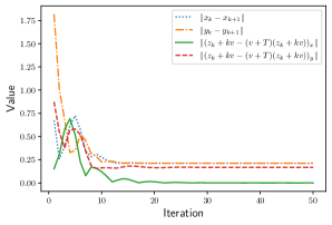
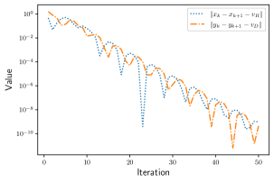
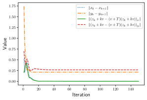
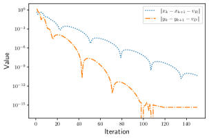
which was given in Example 5.5(i) (respectively Example 5.5(ii)). In this section, we provide numerical illustrations of Theorem 5.10 when applied to LP and QP. Additionally, we numerically verify the conclusion of Example 5.5. For both LP and QP we set $\sigma=\tau=0.3$, ${\bm{x}}_{0}=(0,0)$, ${\bm{y}}_{0}=(0,0,-1,-1)$, and ${\bm{z}}_{0}=({\bm{x}}_{0},{\bm{y}}_{0})^{\mkern-1.5mu\mathsf{T}}$. Finally, following the notation of Theorem 5.10 we set $(\forall{k\in{\mathbb{N}}})$ ${\bm{z}}_{k}=T^{k}{\bm{z}}_{0}$. Let ${k\in{\mathbb{N}}}$. We denote the component of $({\bm{z}}_{k}+k{\bm{v}}-({\bm{v}}+T)({\bm{z}}_{k}+k{\bm{v}}))$ corresponding to ${\bm{x}}_{k}$ (respectively ${\bm{y}}_{k}$) by $({\bm{z}}_{k}+k{\bm{v}}-({\bm{v}}+T)({\bm{z}}_{k}+k{\bm{v}}))_{\bm{x}}$ (respectively $({\bm{z}}_{k}+k{\bm{v}}-({\bm{v}}+T)({\bm{z}}_{k}+k{\bm{v}}))_{\bm{y}}$).

Remark 5.11.

Some comments are in order.

1. Let ${\bm{w}}_{0}\in Z$ and let $Q\colon Z\to Z$ be an affine firmly nonexpansive operator. We set $({\bm{w}}_{k})_{k\in{\mathbb{N}}}=(Q^{k}{\bm{w}}_{0})_{k\in{\mathbb{N}}}$ and we let ${\bm{v}}_{Q}$ be the minimal norm vector in ${\operatorname{ran}}\,(\operatorname{Id}-Q)$. The authors in [9, Theorem 3.2] proved that ${\bm{w}}_{k}+k{\bm{v}}_{Q}$ converges to a point in $\operatorname{Fix}({\bm{v}}_{Q}+Q)$.

2. In view of (i) one wonders if the limit of $({\bm{z}}_{k}+k{\bm{v}})$ lies $\operatorname{Fix}({\bm{v}}+T)$. Our numerical experiments provide a negative answer to this question, which proves the tightness of the conclusion of Theorem 5.10. Indeed, as the plots in Figure 1 and Figure 2 below show, the sequence ${\bm{z}}_{k}+k{\bm{v}}-({\bm{v}}+T)({\bm{z}}_{k}+k{\bm{v}})\to u^{*}\neq{\bm{0}}$. Recalling Theorem 5.10, this in turn implies that ${\bm{z}}_{k}+k{\bm{v}}\to z^{*}\not\in\operatorname{Fix}({\bm{v}}+T)$.

Figure 1: Python plots to illustrate the iterative behavior of PDHG when applied to solve LP. Left: The first $50$ terms of the sequences $(\lVert{\bm{x}}_{k}-{\bm{x}}_{k+1}\rVert)_{k\in{\mathbb{N}}}$ (the blue dotted curve) and $(\lVert{\bm{y}}_{k}-{\bm{y}}_{k+1}\rVert)_{k\in{\mathbb{N}}}$ (the orange dash-dotted curve) are depicted. Also, the first $50$ terms of both components of the sequence $(\lVert{\bm{z}}_{k}+k{\bm{v}}-({\bm{v}}+T)({\bm{z}}_{k}+k{\bm{v}})\rVert)_{k\in{\mathbb{N}}}$ are depicted (the solid green curve and the dashed red curve). Right: The first $50$ terms of the sequences $(\lVert{\bm{x}}_{k}-{\bm{x}}_{k+1}-{\bm{v}}_{R}\rVert)_{k\in{\mathbb{N}}}$ (the orange dotted curve) and $(\lVert{\bm{y}}_{k}-{\bm{y}}_{k+1}-{\bm{v}}_{D}\rVert)_{k\in{\mathbb{N}}}$ (the blue dotted curve) are depicted.

Figure 2: Python plots to illustrate the iterative behavior of PDHG when applied to solve QP. Left: The first $150$ terms of the sequences $(\lVert{\bm{x}}_{k}-{\bm{x}}_{k+1}\rVert)_{k\in{\mathbb{N}}}$ (the blue dotted curve) and $(\lVert{\bm{y}}_{k}-{\bm{y}}_{k+1}\rVert)_{k\in{\mathbb{N}}}$ (the orange dash-dotted curve) are depicted. Also, the first $150$ terms of both components of the sequence $(\lVert{\bm{z}}_{k}+k{\bm{v}}-({\bm{v}}+T)({\bm{z}}_{k}+k{\bm{v}})\rVert)_{k\in{\mathbb{N}}}$ are depicted (the solid green curve and the dashed red curve). Right: The first $150$ terms of the sequences $(\lVert{\bm{x}}_{k}-{\bm{x}}_{k+1}-{\bm{v}}_{R}\rVert)_{k\in{\mathbb{N}}}$ (the orange dotted curve) and $(\lVert{\bm{y}}_{k}-{\bm{y}}_{k+1}-{\bm{v}}_{D}\rVert)_{k\in{\mathbb{N}}}$ (the blue dotted curve) are depicted.

5.5 Computing the infimal displacement vector

In this section, we derive a characterization of ${\operatorname{ran}}\,(\operatorname{Id}-T)$ for 59 as the solution to a system of convex constraints in the case that $K$ is polyhedral. A special case is $K=\mathbb{R}^{m}_{-}$, i.e., QP 78. This formula is useful in case one wants to compute with ${\operatorname{ran}}\,(\operatorname{Id}-T)$, e.g., the determination of the infimal displacement vector via an interior-point method.

We note that Lemma 5.1(vi) already yields such a characterization. However, a naive translation of (vi) to a system of constraints introduces four auxiliary vectors. The following result shows that two auxiliary vectors (denoted ${\bm{w}}$ and ${\bm{y}}$ below) suffice.

Lemma 5.12.

In the setting of Problem 59, suppose that $K$ is a polyhedral cone. Define

$$V:=\left\{({\bm{r}},{\bm{d}})\mbox{$\in X\times Y$}\leavevmode\nobreak\ \Bigg{|}\leavevmode\nobreak\ \exists({\bm{w}},{\bm{y}})\in X\times Y\;\;\mbox{\rm such that}\begin{array}[]{rl}&\frac{1}{\tau}{\bm{d}}-({\cal{A}}{\bm{w}}+{\bm{b}})\in K,\\ &{\bm{y}}-{\bm{d}}\in K^{\ominus},\\ &\frac{1}{\sigma}{\bm{r}}-H{\bm{r}}=-H{\bm{w}}+{\cal{A}}^{\ast}{\bm{y}}+{\bm{c}}\end{array}\right\}.$$ (109)

Then

$$V=M^{-1}({\operatorname{ran}}\,(\partial F+S))={\operatorname{ran}}\,(\operatorname{Id}-T).$$ (110)

Proof. In view of Remark 5.2, it is sufficient to verify the first identity in 110. Let $({\bm{r}},{\bm{d}})\in V$. Then there exists $({\bm{w}},{\bm{y}})\in X\times Y$ such that

$$\begin{array}[]{rl}&\frac{1}{\sigma}{\bm{r}}-{\cal{A}}^{\ast}{\bm{d}}=H{\bm{r}}-H{\bm{w}}+{\cal{A}}^{\ast}{\bm{y}}+{\bm{c}}-{\cal{A}}^{\ast}{\bm{d}}\in{\operatorname{ran}}\,H+{\cal{A}}^{\ast}(K^{\ominus})+{\bm{c}},\\ &\frac{1}{\tau}{\bm{d}}-{\cal{A}}{\bm{r}}=\frac{1}{\tau}{\bm{d}}-({\cal{A}}{\bm{w}}+{\bm{b}})+({\cal{A}}{\bm{w}}+{\bm{b}})-{\cal{A}}{\bm{r}}\in K+{\operatorname{ran}}\,{\cal{A}}+{\bm{b}}.\\ \end{array}$$ (111)

Recalling Remark 5.2, for simplicity we set $R:={\operatorname{ran}}\,(\partial F+S)=({\operatorname{ran}}\,H+{\cal{A}}^{\ast}(K^{\ominus})+{\bm{c}})\times(K+{\operatorname{ran}}\,{\cal{A}}+{\bm{b}})$. The inclusion $V\subseteq M^{-1}R$ follows from the definition of $M$ given in 23 and the nonsingularity of $M$ due to the choices of $\tau,\sigma$. We now show that $M^{-1}R\subseteq V$. Indeed let ${\bm{z}}:=({\bm{z}}_{1},{\bm{z}}_{2})\in R$. Then there exist ${\bm{x}}\in X,{\bm{s}}\in K^{\ominus},{\bm{t}}\in K,{\bm{u}}\in X$ such that

$${\bm{z}}=({\bm{z}}_{1},{\bm{z}}_{2})=(H{\bm{x}}+{\cal{A}}^{\ast}{\bm{s}}+{\bm{c}},{\bm{t}}-{\cal{A}}{\bm{u}}+{\bm{b}}).$$ (112)

We claim that there exist ${\bm{x}}^{*}\in X,{\bm{s}}^{*}\in K^{\ominus},{\bm{t}}^{*}\in K,{\bm{u}}^{*}\in X$ such that

$${\bm{z}}=(H{\bm{x}}^{*}+{\cal{A}}^{\ast}{\bm{s}}^{*}+{\bm{c}},{\bm{t}}^{*}-{\cal{A}}{\bm{u}}^{*}+{\bm{b}})\;\;\text{and}\;\;H{\bm{x}}^{*}=H{\bm{u}}^{*}.$$ (113)

To this end consider the problem:

$$\begin{array}[]{rl}\underset{\begin{subarray}{c}{\overline{\bm{u}}\in X}\end{subarray}}{\mathrm{minimize}}&\tfrac{1}{2}\left\langle{\overline{\bm{u}}},{H\overline{\bm{u}}}\right\rangle-\left\langle{{\bm{z}}_{1}-{\bm{c}}},{\overline{\bm{u}}}\right\rangle\\ \mbox{\rm subject to}&{\cal{A}}\overline{\bm{u}}-{\bm{b}}+{\bm{z}}_{2}\in K.\end{array}$$ (114)

Standard techniques yield that the Lagrangian dual of 114 is

$$\begin{array}[]{rl}\underset{\begin{subarray}{c}{\bar{\bm{s}}\in Y,\bar{\bm{x}}\in X}\end{subarray}}{\mathrm{maximize}}&-\frac{1}{2}\left\langle{\overline{\bm{x}}},{H\overline{\bm{x}}}\right\rangle-\left\langle{{\bm{b}}-{\bm{z}}_{2}},{\overline{\bm{s}}}\right\rangle\\ \mbox{\rm subject to}&-{\cal{A}}^{\ast}\overline{\bm{s}}+{\bm{z}}_{1}-{\bm{c}}=H\overline{\bm{x}}\\ &\overline{\bm{s}}\in K^{\ominus}.\end{array}$$ (115)

It follows from 112 that ${\bm{u}}$ satisfies the primal constraint and the pair $({\bm{x}},{\bm{s}})$ satisfies the dual constraints. Therefore, because $K$ is a polyhedral cone, strong duality holds for the primal-dual problem 114–115 (see, e.g., [15, Comment on Page 227]). Let $({\bm{u}}^{*},({\bm{x}}^{*},{\bm{s}}^{*}))$ denote its primal–dual optimal solution. Then there exists $({\bm{t}}^{*},{\bm{s}}^{*})\in K\times K^{\ominus}$ such that

$${\bm{z}}_{1}=H{\bm{x}}^{*}+{\cal{A}}^{\ast}{\bm{s}}^{*}+{\bm{c}} {\bm{z}}_{2}={\bm{t}}^{*}-{\cal{A}}{\bm{u}}^{*}+{\bm{b}}$$  (dual feasibility)  and    (primal feasibility). (116)

Moreover, strong duality and KKT conditions imply that ${\bm{0}}=H{\bm{u}}^{*}-({\bm{z}}_{1}-{\bm{c}})+{\cal{A}}^{\ast}{\bm{s}}^{*}=H{\bm{u}}^{*}-H{\bm{x}}^{*}.$ This proves 113. Now define $({\bm{r}},{\bm{d}}):=M^{-1}{\bm{z}}$, i.e., $({\bm{z}}_{1},{\bm{z}}_{2})=M({\bm{r}},{\bm{d}})=\left(\tfrac{1}{\sigma}{\bm{r}}-{\cal{A}}^{\ast}{\bm{d}},\tfrac{1}{\tau}{\bm{d}}-{\cal{A}}{\bm{r}}\right)$. This and 116 implies

$$\left(\tfrac{1}{\sigma}{\bm{r}},\tfrac{1}{\tau}{\bm{d}}\right)=(H{\bm{x}}^{*}+{\cal{A}}^{\ast}{\bm{s}}^{*}+{\bm{c}}+{\cal{A}}^{\ast}{\bm{d}},{\bm{t}}^{*}-{\cal{A}}{\bm{u}}^{*}+{\bm{b}}+{\cal{A}}{\bm{r}}).$$ (117)

Define ${\bm{w}}:={\bm{r}}-{\bm{u}}^{*}$ and ${\bm{y}}:={\bm{d}}+{\bm{s}}^{*}$. In view of 113, 117 and 116 we have

$$\begin{array}[]{rl}&\frac{1}{\tau}{\bm{d}}-({\cal{A}}{\bm{w}}+{\bm{b}})={\cal{A}}{\bm{r}}+{\bm{t}}^{*}-{\cal{A}}{\bm{u}}^{*}+{\bm{b}}-({\cal{A}}{\bm{w}}+{\bm{b}})={\bm{t}}^{*}\in K\\ &{\bm{y}}-{\bm{d}}={\bm{s}}^{*}\in K^{\ominus}\\ &\frac{1}{\sigma}{\bm{r}}-H{\bm{r}}={\cal{A}}^{\ast}{\bm{d}}+H{\bm{x}}^{*}+{\cal{A}}^{\ast}{\bm{s}}^{*}+{\bm{c}}-H{\bm{r}}=-H{\bm{w}}+{\cal{A}}^{\ast}{\bm{y}}+{\bm{c}},\end{array}$$

which implies that $({\bm{r}},{\bm{d}})\in V$. The inclusion $M^{-1}R\subseteq V$ follows from the construction $({\bm{r}},{\bm{d}})=M^{-1}{\bm{z}}$. $\hfill\quad\blacksquare$

6 Application to standard conic primal form

In this section, we consider problems of the form 63 under the assumptions

$$C X {\bm{c}}\in X K=\{{\bm{0}}\}$$ is a nonempty closed convex cone of , , and . (118)

In other words, the problem under consideration is:

$$\begin{array}[]{rl}\underset{\begin{subarray}{c}{x\in C}\end{subarray}}{\mathrm{minimize}}&\left\langle{{\bm{c}}},{{\bm{x}}}\right\rangle\\ \mbox{\rm subject to}&{\cal{A}}{\bm{x}}-{\bm{b}}={\bm{0}}.\end{array}$$ (119)

Problem 119 is commonly known as standard conic primal form since it generalizes linear programming in standard equality form, which takes $C=\mathbb{R}^{n}_{+}$. However, the results in this section extend beyond LP since polyhedrality is not assumed. Specializing 66, the PDHG update to solve 119 is

$$\begin{pmatrix}{\bm{x}}^{+}\\ {\bm{y}}^{+}\end{pmatrix}=T\begin{pmatrix}{\bm{x}}\\ {\bm{y}}\end{pmatrix}:=\begin{pmatrix}P_{C}({\bm{x}}-\sigma{\cal{A}}^{*}{\bm{y}}-{\bm{c}})\\ {\bm{y}}+\tau{\cal{A}}(2{\bm{x}}^{+}-{\bm{x}})-\tau{\bm{b}}\end{pmatrix}.$$ (120)

Lemma 6.1.

For 120 we have

$$\overline{\operatorname{ran}}\,(\operatorname{Id}-T)=M^{-1}\Big{(}(\overline{C^{\ominus}+{\operatorname{ran}}\,{\cal{A}}^{*}}+{\bm{c}})\times({\bm{b}}-{\overline{{\cal{A}}(C)}})\Big{)}.$$ (121)

Proof. Recalling 56 and 64, on the one hand we have

$$\operatorname{dom}f=C \operatorname{dom}g=\{{\bm{b}}\} \operatorname{dom}g^{*}=X$$, and . (122)

On the other hand, it follows from [6, Corollary 16.39 and Corollary 16.30], [31, Theorem 3.1] and [6, Corollary 6.50] that

$$\overline{\operatorname{dom}}\ f^{*} =\overline{\operatorname{dom}}\ (\left\langle{{\bm{c}}},{{\bm{x}}}\right\rangle+\iota_{C})^{*}=\overline{\operatorname{dom}}\ \partial(\left\langle{{\bm{c}}},{{\bm{x}}}\right\rangle+\iota_{C})^{*}$$ (123a)

$$=\overline{{\operatorname{ran}}\,}\ \partial(\left\langle{{\bm{c}}},{{\bm{x}}}\right\rangle+\iota_{C})=\overline{{\operatorname{ran}}\,}\ ({\bm{c}}+N_{C})$$ (123b)

$$={\bm{c}}+\overline{{\operatorname{ran}}\,}\ N_{C}={\bm{c}}+C^{\ominus}.$$ (123c)

Now combine 122, 123 and Theorem 3.5(vi). $\hfill\quad\blacksquare$

The following lemma, analogous to Lemma 5.12, presents a parsimonious description of $\overline{\operatorname{ran}}\,(\operatorname{Id}-T)$ via constraints in the context of the standard conic primal form.

Lemma 6.2.

In the setting of Problem 120, define $R:=((C^{\ominus}+{\operatorname{ran}}\,{\cal{A}}^{\ast}+{\bm{c}})\times({\bm{b}}-{\cal{A}}(C)),$ and

$$V:=\left\{({\bm{r}},{\bm{d}})\mbox{$\in X\times Y$}\leavevmode\nobreak\ \Bigg{|}\leavevmode\nobreak\ \mbox{$\exists({\bm{w}},{\bm{y}})\in X\times Y$ \;\;{\rm such that}}\begin{array}[]{rl}&\frac{1}{\tau}{\bm{d}}={\cal{A}}{\bm{w}}+{\bm{b}},\\ &{\bm{r}}-{\bm{w}}\in C,\\ &\frac{1}{\sigma}{\bm{r}}-({\cal{A}}^{\ast}{\bm{y}}+{\bm{c}})\in C^{\ominus}\end{array}\right\}.$$ (124)

Then

$$V=M^{-1}R.\qquad$$ (125)

Proof. Let $({\bm{r}},{\bm{d}})\in V$. Then there exists ${\bm{w}},{\bm{y}}$ such that

$$\begin{array}[]{rl}&\frac{1}{\sigma}{\bm{r}}-{\cal{A}}^{\ast}{\bm{d}}=\frac{1}{\sigma}{\bm{r}}-({\cal{A}}^{\ast}{\bm{y}}+{\bm{c}})+({\cal{A}}^{\ast}{\bm{y}}+{\bm{c}})-{\cal{A}}^{\ast}{\bm{d}}\in C^{\ominus}+{\operatorname{ran}}\,{\cal{A}}^{\ast}+{\bm{c}},\\ &\frac{1}{\tau}{\bm{d}}-{\cal{A}}{\bm{r}}={\cal{A}}({\bm{w}}-{\bm{r}})+{\bm{b}}\in{\bm{b}}-{\cal{A}}(C).\\ \end{array}$$

The inclusion $V\subseteq M^{-1}R$ follows from the definition of $M$ (see 23). We now show that $M^{-1}R\subseteq V$. To this end let ${\bm{z}}\in R$ and define $({\bm{r}},{\bm{d}}):=M^{-1}{\bm{z}}$. Then there exist ${\bm{s}}\in C^{\ominus},{\bm{t}}\in Y,{\bm{u}}\in C$ such that

$${\bm{z}}=({\bm{s}}+{\cal{A}}^{\ast}{\bm{t}}+{\bm{c}},{\bm{b}}-{\cal{A}}{\bm{u}})=\left(\tfrac{1}{\sigma}{\bm{r}}-{\cal{A}}^{\ast}{\bm{d}},\tfrac{1}{\tau}{\bm{d}}-{\cal{A}}{\bm{r}}\right)=M({\bm{r}},{\bm{d}}).$$ (126)

Define ${\bm{w}}:={\bm{r}}-{\bm{u}}$ and ${\bm{y}}:={\bm{d}}+{\bm{t}}$. Combining this with 126 yields

$$\begin{array}[]{rl}&\frac{1}{\tau}{\bm{d}}={\cal{A}}{\bm{r}}+{\bm{b}}-{\cal{A}}{\bm{u}}={\cal{A}}{\bm{w}}+{\bm{b}}\\ &{\bm{r}}-{\bm{w}}={\bm{u}}\in C\\ &\frac{1}{\sigma}{\bm{r}}-({\cal{A}}^{\ast}{\bm{y}}+{\bm{c}})={\cal{A}}^{\ast}{\bm{d}}+{\bm{s}}+{\cal{A}}^{\ast}{\bm{t}}+{\bm{c}}-({\cal{A}}^{\ast}{\bm{y}}+{\bm{c}})={\bm{s}}+{\cal{A}}^{\ast}{\bm{y}}+{\bm{c}}-({\cal{A}}^{\ast}{\bm{y}}+{\bm{c}})\in C^{\ominus},\end{array}$$

which implies that $M^{-1}{\bm{z}}=({\bm{r}},{\bm{d}})\in V$. This completes the proof. $\hfill\quad\blacksquare$

Remark 6.3.

Let $R$ and $V$ be defined as in Lemma 6.2. In view of 121 it is clear that $\overline{\operatorname{ran}}\,(\operatorname{Id}-T)=\overline{V}$.

6.1 Special case: $\ker{\cal{A}}\cap C=\{{\bm{0}}\}$

In this section, we establish that ${\bm{v}}\in{\operatorname{ran}}\,(\operatorname{Id}-T)$ for a subclass of 119. The general version of our result is in Proposition 6.9, and then the general result is specialized to a particular problem class in Section 6.2. We start with the following useful lemma.

Lemma 6.4.

Suppose $X$ finite-dimensional and that $C_{1}$ and $C_{2}$ are nearly convex subsets of $X$ such that $\overline{C_{1}}=\overline{C_{2}}$. Then the following hold.

1. $\operatorname{ri}{C_{1}}=\operatorname{ri}{C_{2}}$.

2. Suppose that $(\exists i\in\{1,2\})$ $C_{i}=X$. Then $C_{1}=C_{2}=X$.

Proof. (i): This is [8, Proposition 2.12]. (ii): Indeed, without loss of generality suppose that $C_{1}=X$. Observe that (i) implies $X=\operatorname{ri}X=\operatorname{ri}C_{1}=\operatorname{ri}C_{2}\subseteq C_{2}\subseteq X$. Hence, $C_{2}=X$ as claimed. $\hfill\quad\blacksquare$

We now have the following corollary which will be used in the sequel.

Corollary 6.5.

Suppose that $X$ is finite-dimensional and that $K_{1}$ and $K_{2}$ are closed convex cones of $X$ such that $K_{1}\cap K_{2}=\{{\bm{0}}\}$. Then $K_{1}^{\ominus}+K_{2}^{\ominus}=X$.

Proof. Indeed, it follows from [27, Corollary 16.4.2.] that $\overline{K_{1}^{\ominus}+K_{2}^{\ominus}}=(K_{1}\cap K_{2})^{\ominus}=\{{\bm{0}}\}^{\ominus}=X$. Now combine this with Lemma 6.4(ii) applied with $C_{1}=K_{1}^{\ominus}+K_{2}^{\ominus}$ and $C_{2}=X$. $\hfill\quad\blacksquare$

Lemma 6.6.

Recalling 120, for Problem 119, the following hold:

1. ${{\bm{v}}_{R}}\in-C$.

2. $\sigma{\cal{A}}^{*}{{\bm{v}}_{D}}=P_{C^{\ominus}}(-{{\bm{v}}_{R}}+\sigma{\cal{A}}^{*}{{\bm{v}}_{D}})\in C^{\ominus}$.

3. $-{{\bm{v}}_{R}}=P_{C}(-{{\bm{v}}_{R}}+\sigma{\cal{A}}^{*}{{\bm{v}}_{D}})\in C$.

4. ${{\bm{v}}_{D}}\in({\cal{A}}(C))^{\ominus}$.

5. Suppose that $\ker{\cal{A}}\cap C=\{{\bm{0}}\}$. Then

   1. ${\bm{v}}_{R}={\bm{0}}$.

   2. $\overline{C^{\ominus}+{\operatorname{ran}}\,{\cal{A}}^{*}}=X$.

Proof. Let ${\bm{z}}_{0}=({\bm{x}}_{0},{\bm{y}}_{0})\in X\times Y$. Update via ${\bm{z}}_{k+1}=T{\bm{z}}_{k}$, where $T$ is defined as in 120. Then

the sequence $$({\bm{x}}_{k})_{k\in{\mathbb{N}}} C$$ lies in . (127)

(i): Because $C$ is a cone, 127 implies that $({\bm{x}}_{k}/k)_{k\geq 1}$ lies in $C$. It follows from 3.8(i) that

$${\bm{x}}_{k}/k\to-{{\bm{v}}_{R}}\in C,$$ (128)

where the inclusion follows from the closedness of $C$. (ii): It follows from 120 applied with ${\bm{x}}$ replaced by ${\bm{x}}_{k}$ and the Moreau decomposition, see, e.g., [6, Theorem 6.30], that

$${\bm{x}}_{k}-{\bm{x}}_{k+1}-\sigma{\cal{A}}^{*}{\bm{y}}_{k}-{\bm{c}}={\bm{x}}_{k}-P_{C}({\bm{x}}_{k}-\sigma{\cal{A}}^{*}{\bm{y}}_{k}-{\bm{c}})-\sigma{\cal{A}}^{*}{\bm{y}}_{k}-{\bm{c}}=P_{C^{\ominus}}({\bm{x}}_{k}-\sigma{\cal{A}}^{*}{\bm{y}}_{k}-{\bm{c}}).$$ (129)

Dividing the above equation by $k\geq 1$, using the positive homogeneity of $P_{C^{\ominus}}$ (see [19, Theorem 5.6(7)]) and taking the limit as $k\to\infty$ in view of 3.8(i)&(ii) and the continuity of $P_{C^{\ominus}}$ we learn that

$$\sigma{\cal{A}}^{*}{{\bm{v}}_{D}}\leftarrow\tfrac{{\bm{x}}_{k}-{\bm{x}}_{k+1}}{k}+\sigma{\cal{A}}^{*}\Big{(}\tfrac{-{\bm{y}}_{k}}{k}\Big{)}-\Big{(}\tfrac{{\bm{c}}}{k}\Big{)}=P_{C^{\ominus}}\Big{(}\tfrac{{\bm{x}}_{k}}{k}+\sigma{\cal{A}}^{*}\big{(}\tfrac{-{\bm{y}}_{k}}{k}\big{)}-\tfrac{{\bm{c}}}{k}\Big{)}\to P_{C^{\ominus}}(-{{\bm{v}}_{R}}+\sigma{\cal{A}}^{*}{{\bm{v}}_{D}}).$$ (130)

That is, $\sigma{\cal{A}}^{*}{{\bm{v}}_{D}}=P_{C^{\ominus}}(-{{\bm{v}}_{R}}+\sigma{\cal{A}}^{*}{{\bm{v}}_{D}})\in C^{\ominus}$. (iii): It follows from Proposition 4.2(iii) that $\left\langle{{{\bm{v}}_{R}}},{{\cal{A}}^{*}{{\bm{v}}_{D}}}\right\rangle=\left\langle{{\cal{A}}{{\bm{v}}_{R}}},{{{\bm{v}}_{D}}}\right\rangle=0$. Now combine this with (i) and (ii) in view of, e.g., [6, Proposition 6.28]. (iv): It follows from (ii) and [6, Proposition 6.37(ii)] that ${{\bm{v}}_{D}}\in({\cal{A}}^{*})^{-1}C^{\ominus}=({\cal{A}}(C))^{\ominus}$. (v)(a): Indeed, (i) and Proposition 4.2(v) yield ${\bm{v}}_{R}\in(-C)\cap\ker{\cal{A}}=-(C\cap\ker{\cal{A}})=\{{\bm{0}}\}$. Hence, ${\bm{v}}_{R}={\bm{0}}$ as claimed. (v)(b): It follows from [6, Fact 2.25(iv) and Proposition 6.35] that $\overline{C^{\ominus}+{\operatorname{ran}}\,{\cal{A}}^{*}}=\overline{C^{\ominus}+\overline{\operatorname{ran}}\,{\cal{A}}^{*}}=\overline{C^{\ominus}+(\ker{\cal{A}})^{\perp}}=\overline{C^{\ominus}+(\ker{\cal{A}})^{\ominus}}=(C\cap\ker{\cal{A}})^{\ominus}=\{{\bm{0}}\}^{\ominus}=X$. The proof is complete. $\hfill\quad\blacksquare$

Before we proceed we recall the following useful fact.

Fact 6.7.

Suppose that $X$ is finite-dimensional and that $\ker{\cal{A}}\cap C=\{{\bm{0}}\}$. Then ${\cal{A}}(C)$ is closed.

Proof. See [27, Theorem 9.1]. $\hfill\quad\blacksquare$

Lemma 6.8.

Suppose that $X$ and $Y$ are finite-dimensional and that $\ker{\cal{A}}\cap C=\{{\bm{0}}\}$. Then for Problem 119 we have:

1. ${\cal{A}}(C)$ is a nonempty closed convex cone.

2. ${C^{\ominus}+{\operatorname{ran}}\,{\cal{A}}^{*}}=X$.

3. $\overline{\operatorname{ran}}\,(\operatorname{Id}-T)=M^{-1}\Big{(}(X\times({\bm{b}}-{{{\cal{A}}(C)}})\Big{)}$.

4. Let ${\bm{z}}\in{\cal{A}}(C)$. Then $\left\langle{{{\bm{v}}_{D}}},{\tfrac{1}{\tau}{{\bm{v}}_{D}}-({\bm{b}}-{\bm{z}})}\right\rangle\leq 0$.

5. $\left\langle{{{\bm{v}}_{D}}},{\tfrac{1}{\tau}{{\bm{v}}_{D}}-{\bm{b}}}\right\rangle\leq 0$.

6. $\tfrac{1}{\tau}{{\bm{v}}_{D}}=P_{{\bm{b}}-{\cal{A}}(C)}({\bm{0}})=P_{({\cal{A}}C)^{\ominus}}({\bm{b}})$.

Let $\overline{{\bm{u}}}\in C$ be such that $\tfrac{1}{\tau}{{\bm{v}}_{D}}={\bm{b}}-{\cal{A}}\overline{{\bm{u}}}$. Then we have

1. $\left\langle{{\cal{A}}\overline{{\bm{u}}}},{{{\bm{v}}_{D}}}\right\rangle=\left\langle{\overline{{\bm{u}}}},{{\cal{A}}^{*}{{\bm{v}}_{D}}}\right\rangle=0$.

2. $\tfrac{1}{\tau}\lVert{{\bm{v}}_{D}}\rVert^{2}=\left\langle{{\bm{b}}},{{{\bm{v}}_{D}}}\right\rangle$.

3. $\overline{{\bm{u}}}=P_{C}(\overline{{\bm{u}}}+{\cal{A}}^{*}{{\bm{v}}_{D}})$ and ${\cal{A}}^{*}{{\bm{v}}_{D}}=P_{C^{\ominus}}(\overline{{\bm{u}}}+{\cal{A}}^{*}{{\bm{v}}_{D}})$.

Proof. (i): Use 6.7 to learn that ${\cal{A}}(C)$ is closed. The convexity is clear because ${\cal{A}}$ is linear and $C$ is convex. The conclusion ${\cal{A}}(C)$ is a cone is straightforward. (ii): Combine Lemma 6.6(v)(b) and Lemma 6.4(ii) applied with with $C_{1}=X$ and $C_{2}=\overline{C^{\ominus}+{\operatorname{ran}}\,{\cal{A}}^{*}}$. (iii): Combine Lemma 6.1, (ii) and (i). (iv): Combine 122 and Proposition 3.10(ii) in view of Lemma 6.6(v)(b). (v): This is a direct consequence of (iv) by setting ${\bm{z}}={\bm{0}}$. (vi): It follows from (iii) in view of 80 that $(-{\cal{A}}^{*}{{\bm{v}}_{D}},\tfrac{1}{\tau}{{\bm{v}}_{D}})=M{\bm{v}}\in X\times({{\bm{b}}-{\cal{A}}(C)})$. That is, $\tfrac{1}{\tau}{{\bm{v}}_{D}}\in{{\bm{b}}-{\cal{A}}(C)}$. Now combine this with (iv) and (i) in view of [6, Theorem 3.16] to learn that $\tfrac{1}{\tau}{{\bm{v}}_{D}}=P_{{\bm{b}}-{\cal{A}}(C)}({\bm{0}})$. Finally, using, e.g., [6, Proposition 3.19] we have

$$\tfrac{1}{\tau}{{\bm{v}}_{D}} =P_{{\bm{b}}-{\cal{A}}(C)}({\bm{0}})={\bm{b}}+P_{-{\cal{A}}(C)}(-{\bm{b}})={\bm{b}}-P_{{\cal{A}}(C)}({\bm{b}})$$ (131a)

$$=(\operatorname{Id}-P_{{\cal{A}}(C)})({\bm{b}})=P_{({\cal{A}}(C))^{\ominus}}({\bm{b}}).$$ (131b)

(vii)&(viii): Indeed, it follows from (v) and Lemma 6.6(ii) that

$$0\leq\left\langle{{\bm{b}}-\tfrac{1}{\tau}{{\bm{v}}_{D}}},{{{\bm{v}}_{D}}}\right\rangle=\left\langle{{\cal{A}}\overline{{\bm{u}}}},{{{\bm{v}}_{D}}}\right\rangle=\left\langle{\overline{{\bm{u}}}},{{\cal{A}}^{*}{{\bm{v}}_{D}}}\right\rangle\leq 0,$$ (132)

hence $\left\langle{{\bm{b}}-\tfrac{1}{\tau}{{\bm{v}}_{D}}},{{{\bm{v}}_{D}}}\right\rangle=\left\langle{{\cal{A}}\overline{{\bm{u}}}},{{{\bm{v}}_{D}}}\right\rangle=\left\langle{\overline{{\bm{u}}}},{{\cal{A}}^{*}{{\bm{v}}_{D}}}\right\rangle=0$ and the conclusion follows. (ix): Combine (vii) and Lemma 6.6(ii) in view of, e.g., [6, Proposition 6.28]. $\hfill\quad\blacksquare$

We now show a sufficient condition to have ${\bm{v}}\in{\operatorname{ran}}\,(\operatorname{Id}-T)$.

Proposition 6.9.

Suppose that $X$ and $Y$ are finite-dimensional, that $\ker{\cal{A}}\cap C=\{{\bm{0}}\}$ and that ${\bm{c}}={\bm{0}}$. Then ${\bm{v}}\in{\operatorname{ran}}\,(\operatorname{Id}-T)$.

Proof. In view of Theorem 3.5(iv) and Lemma 6.6(v)(b) we have

$${\bm{v}}\in{\operatorname{ran}}\,(\operatorname{Id}-T)\Leftrightarrow M{\bm{v}}=\begin{pmatrix}-{\cal{A}}^{*}{{\bm{v}}_{D}}\\ \tfrac{1}{\tau}{{\bm{v}}_{D}}\end{pmatrix}\in{\operatorname{ran}}\,(\partial F+S),$$ (133)

where $\partial F=N_{C}\times\{{\bm{b}}\}$. It follows from Lemma 6.8(vi) that $(\exists\overline{{\bm{u}}}\in{\bf C})$ such that $\tfrac{1}{\tau}{{\bm{v}}_{D}}={\bm{b}}-{\cal{A}}\overline{{\bm{u}}}$. Now consider the point $\begin{pmatrix}\overline{{\bm{u}}}\\ {-{\bm{v}}_{D}}\end{pmatrix}\in C\times Y=\operatorname{dom}\partial F=\operatorname{dom}(\partial F+S)$. We have

$$(\partial F+S)\begin{pmatrix}\overline{{\bm{u}}}\\ {-{\bm{v}}_{D}}\end{pmatrix}=\begin{pmatrix}N_{C}(\overline{{\bm{u}}})-{\cal{A}}^{*}{{\bm{v}}_{D}}\\ {\bm{b}}-{\cal{A}}\overline{{\bm{u}}}\end{pmatrix}\ni\begin{pmatrix}{\bm{0}}-{\cal{A}}^{*}{{\bm{v}}_{D}}\\ {\bm{b}}-{\cal{A}}\overline{{\bm{u}}}\end{pmatrix}=\begin{pmatrix}-{\cal{A}}^{*}{{\bm{v}}_{D}}\\ \tfrac{1}{\tau}{{\bm{v}}_{D}}\end{pmatrix}=M{\bm{v}}.$$ (134)

This completes the proof in view of 133. $\hfill\quad\blacksquare$

Proposition 6.10.

Suppose that $X$ and $Y$ are finite-dimensional, that $\ker{\cal{A}}\cap C=\{{\bm{0}}\}$ and that ${\bm{c}}={\bm{0}}$. Let $({\bm{x}}_{0},{\bm{y}}_{0})\in X\times Y$. Update via $(\forall{k\in{\mathbb{N}}})$

$$({\bm{x}}_{k+1},{\bm{y}}_{k+1})=T({\bm{x}}_{k},{\bm{y}}_{k}).$$ (135)

Then the following hold.

1. The sequence $({\bm{x}}_{k},{\bm{y}}_{k}+k{{\bm{v}}_{D}})_{k\in{\mathbb{N}}}$ is bounded.

Let $\overline{{\bm{x}}}$ be a cluster point of $({\bm{x}}_{k})_{k\in{\mathbb{N}}}$. Then we have

1. $\overline{{\bm{x}}}\in C$.

2. $\tau{\cal{A}}\overline{{\bm{x}}}=\tau{\bm{b}}-{{\bm{v}}_{D}}$.

3. $(\overline{{\bm{x}}},{\bm{0}})\in\operatorname{Fix}({\bm{v}}+T)$.

Proof. (i): Combine Theorem 3.5(ii), and 3.6 in view of Lemma 6.6(v)(a) . (ii): This follows from the fact that $({\bm{x}}_{k})_{k\in{\mathbb{N}}}$ lies in $C$ and $C$ is closed. (iii): Suppose that ${\bm{x}}_{n_{k}}\to\overline{{\bm{x}}}$. It follows from 3.8(i) in view of Theorem 3.5(ii) that ${\bm{x}}_{n_{k}}-{\bm{x}}_{n_{k}+1}\to{\bm{0}}$, hence ${\bm{x}}_{n_{k}+1}\to\overline{{\bm{x}}}$. Therefore, using this and 120 applied with ${\bm{c}}={\bm{0}}$ we have ${{\bm{v}}_{D}}\leftarrow{\bm{y}}_{n_{k}}-{\bm{y}}_{n_{k}+1}=\tau{\bm{b}}-\tau{\cal{A}}(2{\bm{x}}_{n_{k}+1}-{\bm{x}}_{n_{k}})=\tau{\bm{b}}-\tau{\cal{A}}\overline{{\bm{x}}}$. (iv): Indeed, using (ii) and (iii) we have

$${\bm{v}}+T(\overline{{\bm{x}}},{\bm{0}}) =({\bm{0}},{{\bm{v}}_{D}})+(P_{C}(\overline{{\bm{x}}}-\sigma{\cal{A}}^{*}{\bm{0}}),{\bm{0}}+\tau{\cal{A}}(2P_{C}(\overline{{\bm{x}}}-\sigma{\cal{A}}^{*}{\bm{0}})-\overline{{\bm{x}}})-\tau{\bm{b}})$$ (136a)

$$=(\overline{{\bm{x}}},{{\bm{v}}_{D}}+\tau{\cal{A}}\overline{{\bm{x}}}-\tau{\bm{b}})=(\overline{{\bm{x}}},{\bm{0}}),$$ (136b)

and the conclusion follows. $\hfill\quad\blacksquare$

We recall the following fact.

Fact 6.11.

Let $({\bm{z}}_{k})_{k\in{\mathbb{N}}}$ be Fejér monotone with respect to a nonempty closed convex subset $D$ of $X$. Let ${\bm{w}}_{1}$ and ${\bm{w}}_{2}$ be two cluster points of $({\bm{z}}_{k})_{k\in{\mathbb{N}}}$. Then ${\bm{w}}_{1}-{\bm{w}}_{2}\in(D-D)^{\perp}$.

Proof. See, e.g., [7, Lemma 2.2] or [5, Theorem 6.2.2(ii)]. $\hfill\quad\blacksquare$

In the special case considered in this section, namely $\ker{\cal{A}}\cap C=\{{\bm{0}}\}$, ${\bm{c}}={\bm{0}}$, for which we already know ${\bm{v}}_{R}={\bm{0}}$ by Lemma 6.6(v)(a), we can show that the first component of the sequence $({\bm{x}}_{k},{\bm{y}}_{k})_{k\in{\mathbb{N}}}$ converges, and furthermore, we can partly characterize the limit point as follows.

Theorem 6.12.

Suppose that $X$ and $Y$ are finite-dimensional, that $\ker{\cal{A}}\cap C=\{{\bm{0}}\}$ and that ${\bm{c}}={\bm{0}}$. Let $({\bm{x}}_{0},{\bm{y}}_{0})\in X\times Y$. Update via $(\forall{k\in{\mathbb{N}}})$

$$({\bm{x}}_{k+1},{\bm{y}}_{k+1})=T({\bm{x}}_{k},{\bm{y}}_{k}).$$ (137)

Then there exists $\overline{{\bm{x}}}\in C$ such that the following hold.

1. The sequence $({\bm{x}}_{k})_{k\in{\mathbb{N}}}$ converges to $\overline{{\bm{x}}}$.

2. $\overline{{\bm{x}}}\in C\cap L$, where $L=\big{\{}{{\bm{x}}\in X}\leavevmode\nobreak\ \big{|}\leavevmode\nobreak\ {{\cal{A}}{\bm{x}}={\bm{b}}-\tfrac{1}{\tau}{{\bm{v}}_{D}}}\big{\}}$.

Proof. (i): In view of Proposition 6.10(i) it suffices to show that $({\bm{x}}_{k})_{k\in{\mathbb{N}}}$ has at most one cluster point. To this end suppose that $\overline{{\bm{x}}}$ and $\hat{{\bm{x}}}$ are two cluster points of $({\bm{x}}_{k})_{k\in{\mathbb{N}}}$, say ${\bm{x}}_{n_{k}}\to\overline{{\bm{x}}}$ and ${\bm{x}}_{l_{k}}\to\hat{{\bm{x}}}$. After dropping to a subsubsequence and relabelling if needed we can and do assume that ${\bm{z}}_{n_{k}}+n_{k}{\bm{v}}\to(\overline{{\bm{x}}},\overline{{\bm{y}}})$ and ${\bm{z}}_{l_{k}}+l_{k}{\bm{v}}\to(\hat{{\bm{x}}},\hat{{\bm{y}}})$. On the one hand, it follows from Proposition 6.10(iv) that $(\overline{{\bm{x}}},{\bm{0}})$ and $(\hat{{\bm{x}}},{\bm{0}})$ lie in $\operatorname{Fix}({\bm{v}}+T)$. On the other hand, applying 6.11 with $D$ replaced by $\operatorname{Fix}({\bm{v}}+T)$, ${\bm{w}}_{1}$ replaced by $(\overline{{\bm{x}}},\overline{{\bm{y}}})$, and ${\bm{w}}_{2}$ replaced by $(\hat{{\bm{x}}},\hat{{\bm{y}}})$ in view of Proposition 6.10(iii) applied to $\overline{{\bm{x}}}$ and $\hat{{\bm{x}}}$ yields

$$0 =\left\langle{(\overline{{\bm{x}}},\overline{{\bm{y}}})-(\hat{{\bm{x}}},\hat{{\bm{y}}})},{(\overline{{\bm{x}}},{\bm{0}})-(\hat{{\bm{x}}},{\bm{0}})}\right\rangle_{M}$$ (138a)

$$=\left\langle{(\overline{{\bm{x}}}-\hat{{\bm{x}}},\overline{{\bm{y}}}-\hat{{\bm{y}}})},{(\overline{{\bm{x}}}-\hat{{\bm{x}}},{\bm{0}})}\right\rangle_{M}$$ (138b)

$$=\left\langle{(\overline{{\bm{x}}}-\hat{{\bm{x}}},\overline{{\bm{y}}}-\hat{{\bm{y}}})},{(\tfrac{1}{\sigma}(\overline{{\bm{x}}}-\hat{{\bm{x}}})-{\cal{A}}^{*}({\bm{0}}),{\bm{0}}-({\cal{A}}\overline{{\bm{x}}}-{\cal{A}}\hat{{\bm{x}}}))}\right\rangle$$ (138c)

$$=\tfrac{1}{\sigma}\left\langle{(\overline{{\bm{x}}}-\hat{{\bm{x}}},\overline{{\bm{y}}}-\hat{{\bm{y}}})},{(\overline{{\bm{x}}}-\hat{{\bm{x}}},{\bm{0}})}\right\rangle=\tfrac{1}{\sigma}\lVert\overline{{\bm{x}}}-\hat{{\bm{x}}}\rVert^{2}.$$ (138d)

That is $\overline{{\bm{x}}}=\hat{{\bm{x}}}$ and the conclusion follows. (ii): Combine (i) and Proposition 6.10(ii)&(iii). $\hfill\quad\blacksquare$

6.2 Application to the ellipsoid separation problem

An example of Problem 119 in which ${\bm{c}}={\bm{0}}$ and $\ker{\cal{A}}\cap C=\{{\bm{0}}\}$ is the ellipsoid separation problem, which we describe in this section. This problem asks: given two collections of finitely many ellipsoids, say $E_{1},\ldots,E_{k}$ and $E_{1}^{\prime},\ldots,E_{l}^{\prime}$ all lying in $\mathbb{R}^{d}$, is there a hyperplane that strictly separates $E_{1},\ldots,E_{k}$ from $E_{1}^{\prime},\ldots,E_{l}^{\prime}$? This problem is a robust extension of the classic binary classification problem. “Robust” in this context means that the locations of the data points are known only up to an ellipsoid, and that the separating hyperplane should be correct for all possible actual locations of the points. See, e.g., Shivaswamy et al. [29]. We start with a characterization of separators whose proof (omitted) follows directly from the standard hyperplane separation theorem.

Fact 6.13.

Suppose that $X$ is finite-dimensional. Let $E_{1},\ldots,E_{k}$ and $E_{1}^{\prime},\ldots,E_{l}^{\prime}$ be $k+l$ nonempty convex compact bodies lying in $X$. Then there exists $\bm{a}\in X\smallsetminus\{{\bm{0}}\}$, $b\in\mathbb{R}$ such that $\langle\bm{a},{\bm{x}}\rangle<b$ for all ${\bm{x}}\in E_{1}\cup\cdots\cup E_{k}$ and $\langle\bm{a},{\bm{x}}\rangle>b$ for all ${\bm{x}}\in E_{1}^{\prime}\cup\cdots\cup E_{k}^{\prime}$ if and only if $\operatorname{conv}\,(E_{1}\cup\cdots\cup E_{k})\cap\operatorname{conv}\,(E_{1}^{\prime}\cup\cdots\cup E_{l}^{\prime})=\emptyset$.

Let us introduce further notation for the ellipsoids: say that

$$E_{i} :=\{{\bm{x}}\in\mathbb{R}^{d}:\|A_{i}^{-1}({\bm{x}}-{\bm{c}}_{i})\|\leq 1\},\quad i\in\{1,\ldots,k\},$$ (139a)

$$E_{i}^{\prime} :=\{{\bm{x}}\in\mathbb{R}^{d}:\|B_{i}^{-1}({\bm{x}}-{\bm{d}}_{i})\|\leq 1\},\quad i\in\{1,\ldots,l\}.$$ (139b)

Here, $A_{1},\ldots,A_{k},B_{1},\ldots,B_{l}$ are $d\times d$ invertible matrices and ${\bm{c}}_{1},\ldots,{\bm{c}}_{k},{\bm{d}}_{1},\ldots,d_{l}$ are vectors (centers of the ellipsoids). The naive way of writing the problem “Is $\operatorname{conv}\,(E_{1}\cup\cdots\cup E_{k})\cap\operatorname{conv}\,(E_{1}^{\prime}\cup\cdots\cup E_{l}^{\prime})$ nonempty?” would introduce variables ${\bm{v}}_{1},\ldots,{\bm{v}}_{k},{\bm{w}}_{1},\ldots,{\bm{w}}_{l}\in\mathbb{R}^{d}$ constrained to lie in the respective ellipsoids, and nonnegative multipliers $\lambda_{1},\ldots,\lambda_{k},\mu_{1},\ldots,\mu_{l}$ satisfying $\lambda_{1}+\cdots+\lambda_{k}=\mu_{1}+\cdots+\mu_{l}=1$ and $\lambda_{1}{\bm{v}}_{1}+\cdots+\lambda_{k}{\bm{v}}_{k}=\mu_{1}{\bm{w}}_{1}+\cdots+\mu_{l}{\bm{w}}_{l}$. However, this formulation is not convex due to the products $\lambda_{i}{\bm{v}}_{i}$, $\mu_{i}{\bm{w}}_{i}$.

A standard rescaling trick (see., e.g., Boyd & Vandenberghe [15, Exercise 4.56] attributed to Parrilo) reformulates the problem of nonemptiness of the intersection of convex hulls as standard SOCP with variables $\lambda_{1},\ldots,\lambda_{k},\mu_{1},\ldots,\mu_{l},{\bm{p}}_{1},\ldots,{\bm{p}}_{k},{\bm{q}}_{1},\ldots,{\bm{q}}_{l}$:

$$\begin{array}[]{rl}\underset{\begin{subarray}{c}{}\end{subarray}}{\mathrm{minimize}}&0\\ \mbox{\rm subject to}&\lambda_{1}+\cdots+\lambda_{k}=1,\\ &\mu_{1}+\cdots+\mu_{l}=1,\\ &\lambda_{1}{\bm{c}}_{1}+A_{1}{\bm{p}}_{1}+\cdots+\lambda_{k}{\bm{c}}_{k}+A_{k}{\bm{p}}_{k}-\mu_{1}{\bm{d}}_{1}+B_{1}{\bm{q}}_{1}-\cdots-\mu_{l}{\bm{d}}_{l}+B_{l}{\bm{q}}_{l}={\bm{0}},\\ &\|{\bm{p}}_{i}\|\leq\lambda_{i}\quad\forall i\in\{1,\ldots,k\},\\ &\|{\bm{q}}_{i}\|\leq\mu_{i}\quad\forall i\in\{1,\ldots,l\}.\end{array}$$

Note that the constraints $\bm{\lambda}\geq{\bm{0}}$ and $\bm{\mu}\geq{\bm{0}}$ are redundant in this formulation and hence are dropped. The objective “$\min 0$” indicates that any feasible solution to the constraints yields a common point in the convex hulls. Let $X:=\mathbb{R}^{d+1}\times\cdots\times\mathbb{R}^{d+1}$. We further rewrite this problem in the form:

$$\mbox{Find}\;\;{\bm{x}}:=\left(\begin{array}[]{c}\lambda_{1}\\ {\bm{p}}_{1}\\ \vdots\\ \lambda_{k}\\ {\bm{p}}_{k}\\ \mu_{1}\\ {\bm{q}}_{1}\\ \vdots\\ \mu_{l}\\ {\bm{q}}_{l}\end{array}\right)\in X\qquad\mbox{\rm subject to}\;\;\begin{array}[]{rl}&\mathcal{A}{\bm{x}}=\left(\begin{array}[]{c}1\\ 1\\ {\bm{0}}\end{array}\right)=:{\bm{b}},\\ &{\bm{x}}\in C_{2}^{d+1}\times\cdots\times C_{2}^{d+1}=:\bf{C},\end{array}$$ (140)

where $C_{2}^{d+1}$ refers to the second-order cone in $\mathbb{R}^{d+1}$, and where

$$\mathcal{A}=\left(\begin{array}[]{cccccccccc}1&{\bm{0}}^{T}&\cdots&1&{\bm{0}}^{T}&0&{\bm{0}}^{T}&\cdots&0&{\bm{0}}^{T}\\ 0&{\bm{0}}^{T}&\cdots&0&{\bm{0}}^{T}&1&{\bm{0}}^{T}&\cdots&1&{\bm{0}}^{T}\\ {\bm{c}}_{1}&A_{1}&\cdots&{\bm{c}}_{k}&A_{k}&-{\bm{d}}_{1}&B_{1}&\cdots&-{\bm{d}}_{l}&B_{l}\end{array}\right).$$ (141)

This is a convex feasibility problem which can be recast as:

$$\min_{{\bm{x}}\in X}\;\;\iota_{\bf C}({\bm{x}})+\iota_{\{{\bm{0}}\}}({\cal{A}}{\bm{x}}-{\bm{b}}).$$ (142)

By setting $K=\{{\bm{0}}\}$ and $g=\iota_{\bf C}$ in 54 and recalling 120 we learn that the PDHG update for the problem becomes

$$\begin{pmatrix}{\bm{x}}^{+}\\ {\bm{y}}^{+}\end{pmatrix}:=T\begin{pmatrix}{\bm{x}}\\ {\bm{y}}\end{pmatrix}:=\begin{pmatrix}P_{C}({\bm{x}}-\sigma{\cal{A}}^{*}{\bm{y}})\\ {\bm{y}}+\tau{\cal{A}}(2{\bm{x}}^{+}-{\bm{x}})-\tau{\bm{b}}\end{pmatrix}.$$ (143)

Thus, the main work for PDHG in this case is multiplication by ${\cal{A}}$ and ${\cal{A}}^{*}$ and projection onto $\mathbf{C}$.

Lemma 6.14.

We have $\bf{C}\cap\ker{\cal{A}}=(-\bf{C})\cap\ker{\cal{A}}=\{{\bm{0}}\}.$

Proof. It suffices to show $\bf{C}\cap\ker{\cal{A}}=\{0\}.$ Indeed, let ${\bm{z}}=(\lambda_{1},{\bm{p}}_{1},\ldots,\lambda_{k},{\bm{p}}_{k},\mu_{1},{\bm{q}}_{1},\ldots,\mu_{l},{\bm{q}}_{l})\in\bf{C}\cap\ker{\cal{A}}$. On the one hand

$${\bm{z}}\in\bf{C} \Rightarrow (\forall i\in\{1,\ldots,k\}) \lambda_{i}\geq\lVert{\bm{p}}_{i}\rVert\geq 0 (\forall j\in\{1,\ldots,l\}) \mu_{j}\geq\lVert{\bm{q}}_{j}\rVert\geq 0$$ and . (144)

On the other hand

$${\bm{z}}\in\ker{\cal{A}} \Rightarrow \sum_{i=1}^{k}\lambda_{i}=\sum_{j=1}^{l}\mu_{j}=0$$ . (145)

We learn from 144 and 145 that $(\forall i\in\{1,\ldots,k\})$ $\lambda_{i}=0$ and $(\forall j\in\{1,\ldots,l\})$ $\mu_{j}=0$. This, together with 144 yield that $(\forall i\in\{1,\ldots,k\})$ ${\bm{p}}_{i}={\bm{0}}$ and $(\forall j\in\{1,\ldots,l\})$ ${\bm{q}}_{j}={\bm{0}}$. That is ${\bm{z}}={\bm{0}}$ as claimed. The proof is complete. $\hfill\quad\blacksquare$

We have the following two results.

Theorem 6.15.

For Problem 142 we have

1. ${{\bm{v}}_{R}}={\bm{0}}$.

2. ${\bm{v}}\in{\operatorname{ran}}\,(\operatorname{Id}-T)$.

Proof. (i): Combine Lemma 6.14 and Lemma 6.6(v)(a). (ii): Combine Lemma 6.14 and Proposition 6.9. $\hfill\quad\blacksquare$

Lemma 6.16.

Recalling Problem 142, let ${{\bm{v}}_{D}}=(s,t,{\bm{w}})\in\mathbb{R}\times\mathbb{R}\times\mathbb{R}^{d}$ and set ${\cal{A}}^{*}{{\bm{v}}_{D}}=(\lambda_{1},{\bm{p}}_{1},\ldots,\lambda_{k},{\bm{p}}_{k},\mu_{1},{\bm{q}}_{1},\ldots,\mu_{l},{\bm{q}}_{l})$. Then the following hold:

1. ${\bm{w}}={\bm{0}}\Rightarrow{{\bm{v}}_{D}}={\bm{0}}$.

2. ${{\bm{v}}_{D}}\neq{\bm{0}}\Rightarrow s+t>0$.

3. ${{\bm{v}}_{D}}={\bm{0}}\Leftrightarrow{\cal{A}}^{*}{{\bm{v}}_{D}}={\bm{0}}$.

4. Suppose that $0\in\{\lambda_{1},\ldots,\lambda_{k},\mu_{1},\ldots,\mu_{l}\}$. Then ${{\bm{v}}_{D}}={\bm{0}}$.

5. Suppose that ${\bm{0}}\in\{{\bm{p}}_{1},\ldots,{\bm{p}}_{k},{\bm{q}}_{1},\ldots,{\bm{q}}_{l}\}$. Then ${{\bm{v}}_{D}}={\bm{0}}$.

Proof. It follows from Lemma 6.8(viii) that

$$s+t=\tfrac{1}{\tau}(s^{2}+t^{2}+\lVert{\bm{w}}\rVert^{2})\geq 0.$$ (146)

(i): Indeed, Lemma 6.6(ii) implies that $\lVert{\bm{p}}_{1}\rVert=\lVert A_{1}^{*}{\bm{w}}\rVert\leq-\lambda_{1}=-s-\left\langle{{\bm{c}}},{{\bm{w}}}\right\rangle$ and similarly $\lVert B_{1}^{*}{\bm{w}}\rVert\leq-t+\left\langle{d},{{\bm{w}}}\right\rangle$. Consequently, ${\bm{w}}={\bm{0}}$ $\Rightarrow$ $s\leq 0$ and $t\leq 0$. In view of 146 we conclude that $s+t=0$ and hence $s^{2}+t^{2}=0$, equivalently, $s=t=0$. That is ${{\bm{v}}_{D}}={\bm{0}}$. (ii): Combine (i) and 146. (iii): “$\Rightarrow$”: This is clear. “$\Leftarrow$”: Observe that, because $A_{1}$ is invertible and $A_{1}^{*}{\bm{w}}={\bm{0}}$ we must have ${\bm{w}}={\bm{0}}$. Now combine this with (i). (iv): Without loss of generality, we may and do assume that $\lambda_{1}=0$. Then ${\bm{p}}_{1}=A_{1}^{*}{\bm{w}}={\bm{0}}$, hence ${\bm{w}}={\bm{0}}$. Now combine this with (i). (v): Without loss of generality, we may and do assume that ${\bm{p}}_{1}=A_{1}^{*}{\bm{w}}={\bm{0}}$. Then ${\bm{w}}={\bm{0}}$ and the conclusion follows in view of (i). $\hfill\quad\blacksquare$

Theorem 6.17.

Recalling Problem 142, let $T$ be defined as in 143. Let ${\bm{x}}_{0}\in\mathbb{R}^{d+1}\times\ldots\times\mathbb{R}^{d+1}$ and let ${\bm{y}}_{0}\in\mathbb{R}^{d+2}$. Update via $(\forall{k\in{\mathbb{N}}})$

$$({\bm{x}}_{k+1},{\bm{y}}_{k+1})=T({\bm{x}}_{k},{\bm{y}}_{k}).$$ (147)

Then there exists $\overline{{\bm{x}}}\in C$ such that the following hold.

1. The sequence $({\bm{x}}_{k})_{k\in{\mathbb{N}}}$ converges to $\overline{{\bm{x}}}$.

2. $\overline{{\bm{x}}}\in{\bf C}\cap L$, where $L=\big{\{}{{\bm{x}}\in\mathbb{R}^{d+1}\times\ldots\mathbb{R}^{d+1}}\leavevmode\nobreak\ \big{|}\leavevmode\nobreak\ {{\cal{A}}{\bm{x}}={\bm{b}}-\tfrac{{\bm{v}}_{D}}{\tau}}\big{\}}$.

Proof. (i)–(ii): Combine Lemma 6.14 and Theorem 6.12(i)&(ii). $\hfill\quad\blacksquare$

As indicated by 6.13, disjointness of the convex hulls, i.e., primal infeasibility of 140, is certified by a separating hyperplane. Furthermore, we know from Theorem 6.15 that ${\bm{v}}_{D}\neq{\bm{0}}$ in the infeasible case. We now argue a nonzero ${\bm{v}}_{D}$ encodes a separating hyperplane. We first characterize such a hyperplane with the following lemma.

Lemma 6.18.

Given invertible $A\in\mathbb{R}^{n\times n}$, ${\bm{c}}\in\mathbb{R}^{n}$, $s\in\mathbb{R}$ and ${\bm{w}}\in\mathbb{R}^{n}\smallsetminus\{{\bm{0}}\}$, consider the ellipsoid $E:=\big{\{}{{\bm{x}}\in\mathbb{R}^{n}}\leavevmode\nobreak\ \big{|}\leavevmode\nobreak\ {\|A^{-1}({\bm{x}}-{\bm{c}})\|\leq 1}\big{\}}$ and the halfspace $H:=\big{\{}{{\bm{x}}\in\mathbb{R}^{n}}\leavevmode\nobreak\ \big{|}\leavevmode\nobreak\ {\langle{\bm{w}},{\bm{x}}\rangle\leq s}\big{\}}.$ The following hold.

1. $E\subseteq H$ $\Leftrightarrow$ $s\geq\|A^{*}{\bm{w}}\|+\langle{\bm{c}},{\bm{w}}\rangle.$

2. $E\subseteq\operatorname{int}H$ $\Leftrightarrow$ $s>\|A^{*}{\bm{w}}\|+\langle{\bm{c}},{\bm{w}}\rangle.$

Proof. Let ${\bm{x}}\in\mathbb{R}^{n}$. Then

$$\langle{\bm{w}},{\bm{x}}\rangle=\langle{\bm{w}},{\bm{x}}-{\bm{c}}\rangle+\langle{\bm{w}},{\bm{c}}\rangle=\langle A^{*}{\bm{w}},A^{-1}({\bm{x}}-{\bm{c}})\rangle+\langle{\bm{w}},{\bm{c}}\rangle.$$ (148)

(i): $``\Leftarrow"$: Let ${\bm{x}}\in E$. Using 148 and Cauchy–Schwarz we have $\langle{\bm{w}},{\bm{x}}\rangle\leq\|A^{*}{\bm{w}}\|\cdot\|A^{-1}({\bm{x}}-{\bm{c}})\|+\langle{\bm{w}},{\bm{c}}\rangle\leq\|A^{*}{\bm{w}}\|+\langle{\bm{w}},{\bm{c}}\rangle\leq s$. $``\Rightarrow"$: Let ${\bm{x}}=A(A^{*}{\bm{w}}/\lVert A^{*}{\bm{w}}\rVert)+{\bm{c}}$. Then ${\bm{x}}\in E$, hence ${\bm{x}}\in H$ and 148 implies $s\geq\langle{\bm{w}},{\bm{x}}\rangle=\langle A^{*}{\bm{w}},A^{-1}({\bm{x}}-{\bm{c}})\rangle+\langle{\bm{w}},{\bm{c}}\rangle=\lVert A^{*}{\bm{w}}\rVert+\langle{\bm{w}},{\bm{c}}\rangle.$ (ii): The proof proceeds similar to the proof of (i). $\hfill\quad\blacksquare$

We now state and prove our main result for the ellipsoid separation problem, which states that, because ${\bm{v}}\in{\operatorname{ran}}\,(\operatorname{Id}-T)$ (Theorem 6.15(ii)), a nonzero ${\bm{v}}$ indicates inconsistency, and furthermore, a nonzero ${\bm{v}}$ encodes a strict separating hyperplane.

Theorem 6.19.

Given $k+l$ ellipsoids specified by 139, let ${\bm{v}}_{D}=:(s,t,{\bm{w}})$ and recall 143. Then the following are equivalent.

1. $\operatorname{conv}\,(E_{1}\cup\cdots\cup E_{k})\cap\operatorname{conv}\,(E_{1}^{\prime}\cup\cdots\cup E^{\prime}_{l})=\emptyset$,

2. SOCP problem 140 is infeasible,

3. ${\bm{0}}\notin{\operatorname{ran}}\,(\operatorname{Id}-T)$, where $T$ is the PDHG operator given by 143,

4. ${\bm{v}}\neq{\bm{0}}$,

5. ${\bm{v}}_{D}\neq{\bm{0}}$,

6. $s>-t$.

Any one of these statements implies:

1. The hyperplane $\big{\{}{{\bm{x}}}\leavevmode\nobreak\ \big{|}\leavevmode\nobreak\ {\langle{\bm{w}},{\bm{x}}\rangle=s^{\prime}}\big{\}}$ strictly separates $E_{1},\ldots,E_{k}$ from $E_{1}^{\prime},\ldots,E_{l}^{\prime}$, where $s^{\prime}$ is chosen arbitrarily in $\left]-t,s\right[$.

Conversely, the existence of $({\bm{w}},s^{\prime})$ as in (vii) implies all of (i)–(vi).

Proof. (i)$\Leftrightarrow$ (ii): This was explained earlier in the formulation of 140. (ii)$\Leftrightarrow$(iii): We show the contrapositives. If 140 has a solution say ${\bm{x}}^{*}$, then $({\bm{x}}^{*},{\bm{0}})$ is a fixed point of $T$ defined in 143. Equivalently, ${\bm{0}}\in{\operatorname{ran}}\,(\operatorname{Id}-T)$. Conversely, suppose that $({\bm{x}},{\bm{y}})\in\operatorname{Fix}T$. Then ${\bm{x}}\in\mathbf{C}$ and ${\cal{A}}{\bm{x}}={\bm{b}}$, i.e., ${\bm{x}}$ solves 140. (iii)$\Leftrightarrow$(iv): This follows from Theorem 6.15(ii). (iv)$\Leftrightarrow$(v): This follows from Theorem 6.15(i). (v)$\Leftrightarrow$(vi): The forward direction is established by Lemma 6.16(ii), while the reverse direction is trivial. (vi)$\Rightarrow$(vii): Recalling the form of ${\cal{A}}$ in 141, we have

$${\cal{A}}^{*}{\bm{v}}_{D}=\left(\begin{array}[]{c}s+\langle{\bm{c}}_{1},{\bm{w}}\rangle\\ A_{1}^{*}{\bm{w}}\\ \vdots\\ s+\langle{\bm{c}}_{k},{\bm{w}}\rangle\\ A_{k}^{*}{\bm{w}}\\ t-\langle{\bm{d}}_{1},{\bm{w}}\rangle\\ B_{1}^{*}{\bm{w}}\\ \vdots\\ t-\langle{\bm{d}}_{l},{\bm{w}}\rangle\\ B_{l}^{*}{\bm{w}}\end{array}\right).$$

By Lemma 6.6(ii), we know that ${\cal{A}}^{*}{\bm{v}}_{D}\in\mathbf{C}^{\ominus}$, in other words,

$$-s-\langle{\bm{c}}_{i},{\bm{w}}\rangle \geq\|A_{i}^{*}{\bm{w}}\|,\quad i\in\{1,\ldots,k\},$$

$$-t+\langle{\bm{d}}_{i},{\bm{w}}\rangle \geq\|B_{i}^{*}{\bm{w}}\|,\quad i\in\{1,\ldots,l\}.$$

Since $s>-t$, select an arbitrary $s^{\prime}$ satisfying $s>-s^{\prime}>-t$. Then we obtain the inequalities

$$s^{\prime} >\|A_{i}^{*}{\bm{w}}\|+\langle{\bm{c}}_{i},{\bm{w}}\rangle,\quad i\in\{1,\ldots,k\},$$

$$-s^{\prime} >\|B_{i}^{*}{\bm{w}}\|+\langle{\bm{d}}_{i},-{\bm{w}}\rangle,\quad i\in\{1,\ldots,l\}.$$

In view of Lemma 6.18, these inequalities show that $E_{1},\ldots,E_{k}$ are strictly on one side of the hyperplane $\big{\{}{{\bm{x}}}\leavevmode\nobreak\ \big{|}\leavevmode\nobreak\ {\langle{\bm{w}},{\bm{x}}\rangle=s^{\prime}}\big{\}}$ while $E_{1}^{\prime},\ldots,E_{l}^{\prime}$ are strictly on the other side, thus establishing (vii). Finally, the converse statement at the end of the theorem follows from 6.13. $\hfill\quad\blacksquare$

7 Conclusion

We have developed a new formula for $\overline{\operatorname{ran}}\,(\operatorname{Id}-T)$ when $T$ is the PDHG operator. We applied this formula to quadratic programming and the ellipsoid separation problem to show that in both cases, PDHG can diagnose inconsistency by checking the limiting value of ${\bm{z}}_{k}-{\bm{z}}_{k+1}$ as per 3.8(ii). Both results used the conclusion that ${\bm{v}}\in{\operatorname{ran}}\,(\operatorname{Id}-T)$, where ${\bm{v}}$ is the infimal displacement vector. We provided new results on the convergence of PDHG iterates for both problems. Many issues remain in understanding the landscape of PDHG for infeasible conic optimization problems. Lest the reader suspect that 3.8(ii) can always diagnose inconsistency, we point out that it is relatively easy to construct small contrived inconsistent problems such that ${\bm{0}}\in\overline{\operatorname{ran}}\,(\operatorname{Id}-T)\smallsetminus{\operatorname{ran}}\,(\operatorname{Id}-T)$, meaning that the test based on 3.8(ii) will fail to detect inconsistency. There are also realistic examples when this occurs, for example, the unbounded case of the min-volume-ellipsoid problem (see, e.g., formulation (12a) in [30]), which arises when the data points lie in a low-dimensional affine space.

References

- [1] David Applegate, Mateo Díaz, Haihao Lu, and Miles Lubin. Infeasibility detection with primal-dual hybrid gradient for large-scale linear programming. https://arxiv.org/abs/2102.04592, 2021.
- [2] J. B. Baillon, R. E. Bruck, and S. Reich. On the asymptotic behavior of nonexpansive mappings and semigroups in Banach spaces. Houston Journal of Mathematics, 4:1–9, 1978.
- [3] Goran Banjac. On the minimal displacement vector of the Douglas–Rachford operator. Operations Research Letters, 49(2):197–200, 2021.
- [4] Sedi Bartz, Heinz H. Bauschke, Jonathan M. Borwein, Simeon Reich, and Xianfu Wang. Fitzpatrick functions, cyclic monotonicity and Rockafellar’s antiderivative. Nonlinear Analysis: Theory, Methods & Applications, 66(5):1198–1223, 2007.
- [5] Heinz H. Bauschke. Projection Algorithms and Monotone Operators. PhD thesis, Simon Fraser University, Burnaby, B.C., Canada, 1996.
- [6] Heinz H. Bauschke and Patrick L. Combettes. Convex analysis and monotone operator theory in Hilbert spaces. Springer, 2 edition, 2017.
- [7] Heinz H. Bauschke, Minh N. Dao, and Walaa M. Moursi. On Fejér monotone sequences and nonexpansive mappings. Linear and Nonlinear Analysis, 1:287–295, 2015.
- [8] Heinz H Bauschke, Sarah M Moffat, and Xianfu Wang. Near equality, near convexity, sums of maximally monotone operators, and averages of firmly nonexpansive mappings. Mathematical Programming Series B, 139:55–70, 2013.
- [9] Heinz H. Bauschke and Walaa M. Moursi. The Douglas–Rachford algorithm for two (not necessarily intersecting) affine subspaces. SIAM Journal on Optimization, 26(2):968–985, 2016.
- [10] Heinz H. Bauschke and Walaa M. Moursi. On the Douglas–Rachford algorithm. Mathematical Programming Series A, 164:263–284, 2017.
- [11] Heinz H. Bauschke and Walaa M. Moursi. On the Douglas–Rachford algorithm for solving possibly inconsistent optimization problems. Mathematics of Operations Research, 2023. https://doi.org/10.1287/moor.2022.1347.
- [12] Radu Ioan Bot. Conjugate duality in convex optimization, volume 637 of Lecture Notes in Economics and Mathematical Systems. Springer Science & Business Media, 2009.
- [13] Radu Ioan Bot, Sorin-Mihai Grad, and Gert Wanka. Duality in vector optimization. Springer Science & Business Media, 2009.
- [14] Radu Ioan Bot and Christopher Hendrich. A Douglas–Rachford type primal-dual method for solving inclusions with mixtures of composite and parallel-sum type monotone operators. SIAM Journal on Optimization, 23(4):2541–2565, 2013.
- [15] Stephen Boyd and Lieven Vandenberghe. Convex Optimization. Cambridge University Press, 2004.
- [16] Luis M. Briceño Arias and Patrick L. Combettes. A monotone+skew splitting model for composite monotone inclusions in duality. SIAM Journal on Optimization, 21(4):1230–1250, 2011.
- [17] R.E. Bruck and S. Reich. Nonexpansive projections and resolvents of accretive operators in Banach spaces. Houston Journal of Mathematics, 3:459–470, 1977.
- [18] Antonin Chambolle and Thomas Pock. A first-order primal-dual algorithm for convex problems with applications to imaging. Journal of Mathematical Imaging and Vision, 40(1):120–145, 2011.
- [19] Frank Deutsch. Best Approximation in Inner Product Spaces. Springer, 2001.
- [20] Yanli Liu, Ernest K Ryu, and Wotao Yin. A new use of Douglas–Rachford splitting for identifying infeasible, unbounded, and pathological conic programs. Mathematical Programming Series A, 177(1-2):225–253, 2019.
- [21] Haihao Lu. First-order methods for linear programming: Theory and computation. Cornell University Operations Research and Information Engineering Colloquium, https://www.youtube.com/watch?v=l5kR6I6zesA, 2022.
- [22] Walaa M. Moursi. The Douglas–Rachford operator in the possibly inconsistent case: static properties and dynamic behaviour. PhD thesis, University of British Columbia, 2016. https://doi.org/10.14288/1.0340501.
- [23] Walaa M. Moursi. The forward–backward algorithm and the normal problem. Journal of Optimization Theory and Applications, 176:605–624, 2018.
- [24] Daniel O’Connor and Lieven Vandenberghe. On the equivalence of the primal-dual hybrid gradient method and Douglas–Rachford splitting. Mathematical Programming, 179(1-2):85–108, 2020.
- [25] A Pazy. Asymptotic behavior of contractions in Hilbert space. Israel Journal of Mathematics, 9:235–240, 1971.
- [26] Stephen M. Robinson. Some continuity properties of polyhedral multifunctions. In H. König, B. Korte, and K. Ritter, editors, Mathematical Programming at Oberwolfach, pages 206–214. Springer, 1980.
- [27] R Tyrrell Rockafellar. Convex analysis, volume 11. Princeton University Press, 1970.
- [28] Ernest K Ryu, Yanli Liu, and Wotao Yin. Douglas–Rachford splitting and ADMM for pathological convex optimization. Computational Optimization and Applications, 74(3):747–778, 2019.
- [29] Pannagadatta K Shivaswamy, Chiranjib Bhattacharyya, and Alexander J Smola. Second order cone programming approaches for handling missing and uncertain data. Journal of Machine Learning Research, pages 1283–1314, 2006.
- [30] Michael J. Todd and E. Alper Yıldırım. On Khachiyan’s algorithm for the computation of minimum-volume enclosing ellipsoids. Discrete Applied Mathematics, 155(13):1731–1744, 2007.
- [31] Eduardo H Zarantonello. Projections on convex sets in Hilbert space and spectral theory: Part I. projections on convex sets: Part II. spectral theory. In Eduardo H Zarantonello, editor, Contributions to nonlinear functional analysis, pages 237–424. Elsevier, 1971.