Percolation-induced PT symmetry breaking
Abstract
We propose a new avenue in which percolation, which has been much associated with critical phase transitions, can also dictate the asymptotic dynamics of non-Hermitian systems by breaking PT symmetry. Central to it is our newly-designed mechanism of topologically guided gain, where chiral edge wavepackets in a topological system experience non-Hermitian gain or loss based on how they are topologically steered. For sufficiently wide topological islands, this leads to irreversible growth due to positive feedback from interlayer tunneling. As such, a percolation transition that merges small topological islands into larger ones also drives the edge spectrum across a real to complex transition. Our discovery showcases intriguing dynamical consequences from the triple interplay of chiral topology, directed gain and interlayer tunneling, and suggests new routes for the topology to be harnessed in the control of feedback systems.
In a non-Hermitian system, the reality of the spectrum crucially controls the long-time dynamics. Even under strong gain or loss, non-Hermitian real spectra and non-divergent time evolution are still possible if PT symmetry remains unbroken [1, 2, 3]. This has been extensively studied and achieved through careful control of gain/loss, coupling strengths and external applied fields [4, 5, 6, 7, 8, 9, 10, 11, 12, 13, 14, 15, 16, 17, 18, 19, 20, 21, 22, 23, 24]. In optics, for instance, tuning the gain-loss contrast or the refractive index can result in unidirectional invisibility [9, 11, 12, 15], power oscillations [5, 6, 7, 8, 10], non-reciprocal transmission [14, 22, 24, 23] and enhanced sensing [17, 19, 20, 23].
In this work, we unveil a new route for PT symmetry breaking where the asymptotic dynamics in a disordered non-Hermitian system is controlled by the percolation transition of its real-space texture. While percolation has been extensively linked to second-order phase transitions [25, 26, 27, 28, 29], conformal field theory [30, 31, 32], Schramm-Loewner Evolutions [33, 34, 35, 36] and other critical phenomena [26, 37, 38, 39], percolation itself has never been found to control long-time non-Hermitian dynamics [40, 41, 42, 43].
Central to our percolation-induced PT symmetry breaking is the newly-designed mechanism of topologically guided gain/loss. Unlike in usual non-Hermitian skin effect (NHSE) [44, 45, 46, 47, 48, 49, 50, 51, 52, 53, 54, 55, 56, 57, 58, 59, 60, 61, 62, 63, 64, 65, 66, 67, 68, 69] systems where wavepackets simple spread out and are amplified asymmetrically due to directed amplification, wavepackets in our protocol are steered by chiral topological pumping which controls the extent of gain/loss. By weakly coupling two Chern topological layers with oppositely directed gain, this topological guiding mechanism can induce a PT transition when a sufficiently wide distance is traversed – in the disordered context, this leads to a percolation-induced PT transition as small topological islands coalesce into larger ones. Through this, percolation thus becomes a control knob for the PT transition from oscillatory to divergent dynamics. We note that our mechanism, which relies on chiral topologically guided gain, is completely distinct from the well-known complex-real spectral transition induced by the NHSE [48, 49, 50, 51], where a boundary blocks directionally pumped state from further gain.
In this work, we first introduce topologically guided gain in a model-independent setting, and then demonstrate its excellent agreement with numerical results when specialized to a bilayer non-Hermitian Chern model. Building upon this foundation, we next show that it instigates a percolation-induced PT phase transition among disordered topological islands.
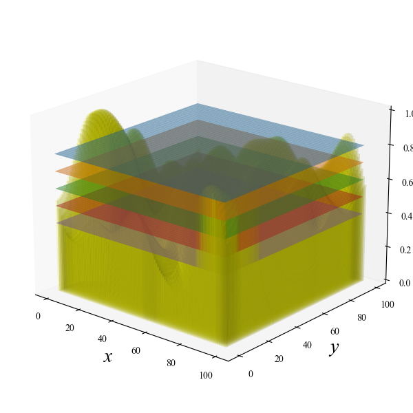
Size-dependent PT edge transition from topologically guided gain.– To understand how a percolation transition can break PT symmetry, we first examine how a single topological island can exhibit PT symmetry breaking when it becomes sufficiently wide. For simplicity, consider an island defined by a rectangular lattice with open boundaries (Fig. 1). In emphasizing the generic nature of topologically guided gain, we shall not specialize to any particular model yet but only stipulate the following 3 necessary ingredients: (i) chiral topological edge modes of velocity , (ii) directed amplification of strength , and (iii) presence of weak interlayer tunneling rate in a minimal bilayer structure. In Fig. 1, we depict how the dynamical evolution of edge wavepackets, initialized at time in the upper left corner, is controlled by the triple interplay of these ingredients.
To build intuition, we first consider only a single Chern layer of width and height (Fig. 1(a)), which harbor the first two ingredients of Chern topology and asymmetric gain/loss. An edge wavepacket is chirally pumped clockwise along the rectangular boundaries at a constant speed , remaining confined and preserving its shape even after completing a boundary loop [70, 71, 72, 73]. If the lattice hoppings were made uniformly asymmetric in one direction (WLOG, horizontally), this edge circulation still remains unitary despite the non-Hermiticity, since the hopping asymmetry can be “gauged out” by redefining the real-space basis [19, 46, 48, 59]. If the left hoppings are stronger than the right hoppings by a factor of , the asymmetry can be removed by rescaling the basis orbital at site by , . Hence the wavepacket is simply attenuated by as it is chirally propagated to the right boundary, and grows back to its original magnitude when it returns to the left boundary. Overall, there is thus no net gain after each chiral loop around a single layer.
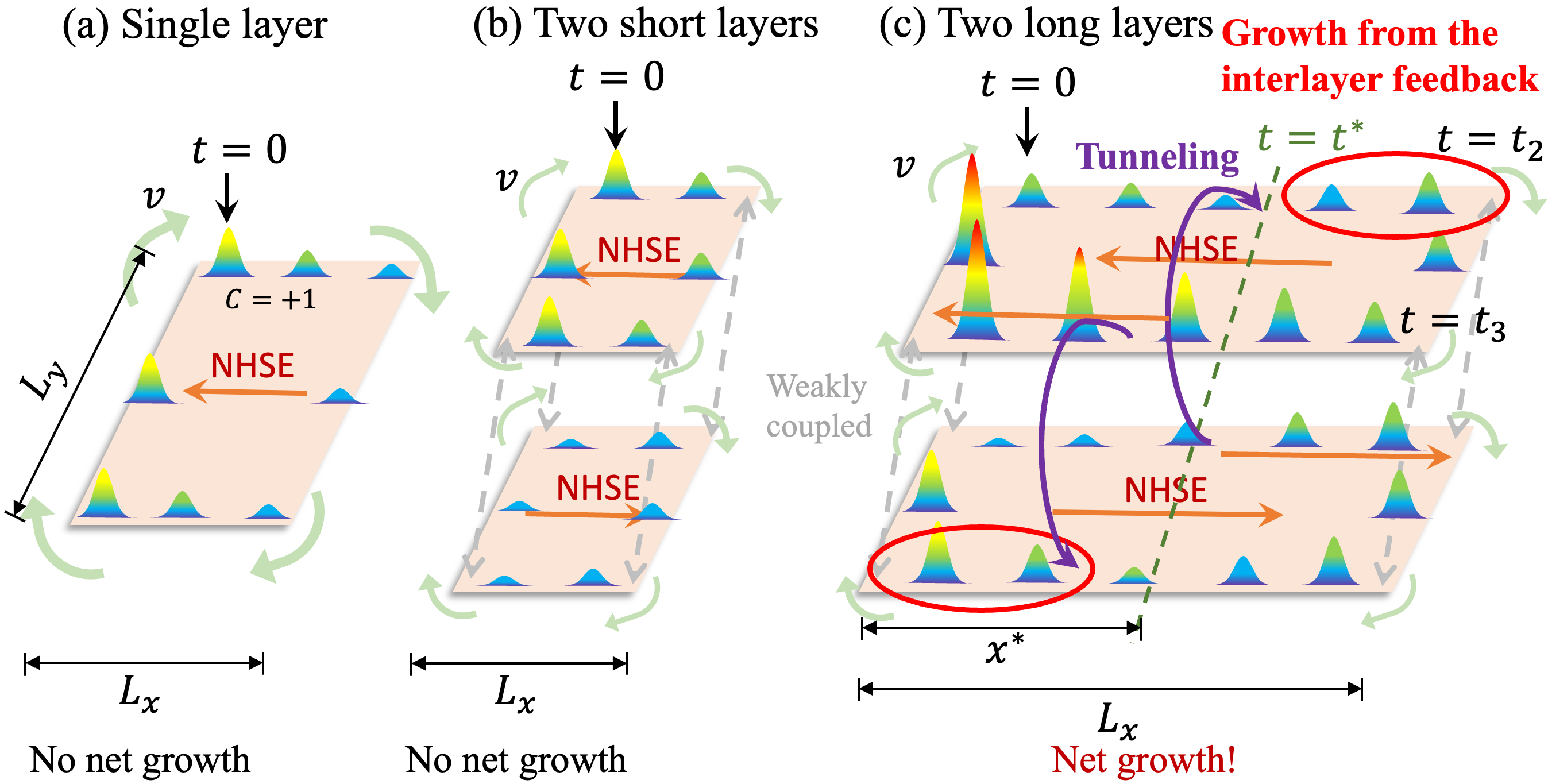
We next introduce the third ingredient of weak interlayer tunneling and show how it can lead to topologically guided gain. We weakly couple two clockwise chiral Chern layers with oppositely hopping asymmetries (Fig. 1(b,c)). For very weak , wavepackets continue to evolve independently in each layer, as in Fig. 1(b).
But interestingly, when or the island width is sufficiently large 111But still with much smaller than the topological gap., positive feedback growth is possible due to interlayer tunneling. In Fig. 1(c), the initial wavepacket only has nonzero amplitude in the upper layer. Due to interlayer tunneling, it quickly induces a small amplitude in the lower layer. Even though may initially be very weak, it chirally propagates to the right and is thus amplified exponentially viz. . By contrast, decays exponentially in the upper layer due to its opposite . For sufficiently large or , there would exist a point where has decayed so much that it becomes dominated by the tunneling from the growing : this occurs when i.e.
| (1) |
After , wavepackets in both layers universally experience exponential gain since the growth is now dominated by the growing lower-layer wavepacket . The gain stops only at when both wavepackets have arrived at the right boundary, where . After chiral propagating to the lower right corner at , the above process repeats with the roles of the upper and lower layer wavepackets reversed, leading to another stationary point in the wavepacket decay (now of ) at . In all, after completing one loop around the island boundary, we have , which is a net gain. Modeled as non-Hermitian stroboscopic time evolution , where each period lasts for a time interval of , this gain corresponds to a complex energy with
| (2) |
when , and zero otherwise. Just from purely heuristic arguments, independent of model details, we have managed to show how the triple interplay of chiral topology, directed gain and interlayer tunneling can break edge PT symmetry proportionally to the velocity of the chiral edge modes, and the gain asymmetry . Remarkably, the dynamical gain rate is also strongly dependent on the island width and aspect ratio, although in a manner distinct from the critical skin effect [57, 75, 76, 77], which does not employ any topological guiding to control the spreading of wavepackets.
For a concrete demonstration of topologically guided gain, we next specialize in a coupled bilayer system where each layer is given by the well-known QWZ Chern model [78] with non-Hermitian asymmetry introduced into every other hopping in the -direction [79]:
| (3) | ||||
where such that the Chern number is , and and the Pauli matrices in the sublattice basis. The interlayer coupling is expected to be proportional to the interlayer tunneling rate , which we shall later determine empirically. With , the directed gain is towards the left(right) in the upper(lower) layer. Confined by boundaries in both directions under a rectangular geometry, this directed gain modifies the energy dispersion to , with , as determined by the generalized Brillouin zone [80, 79, 48].
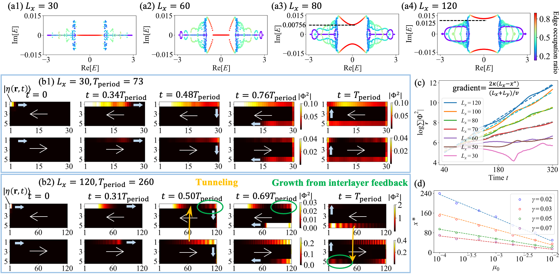
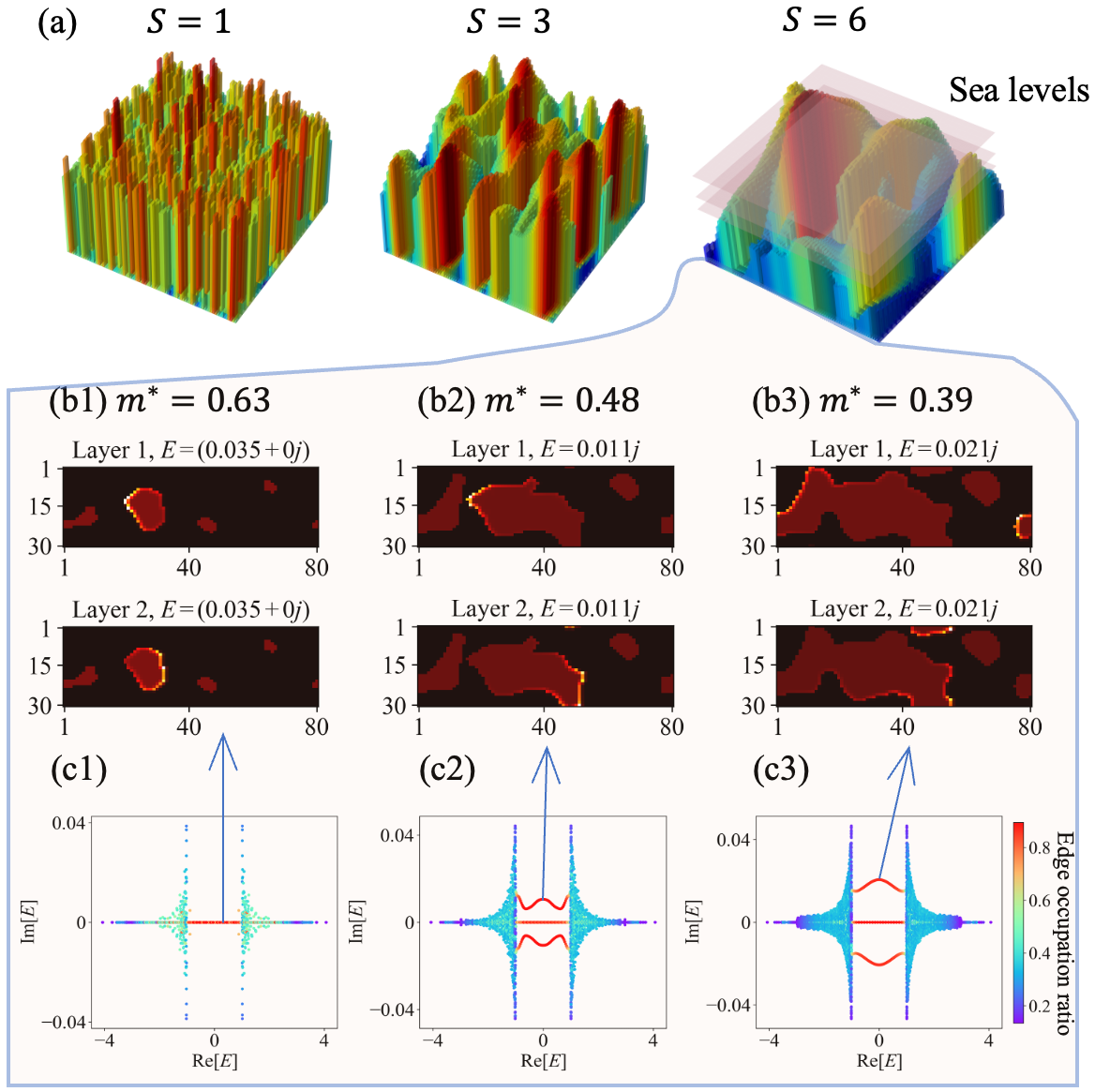
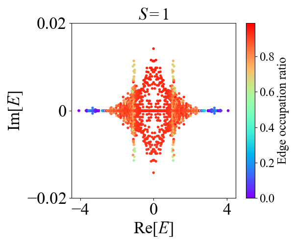
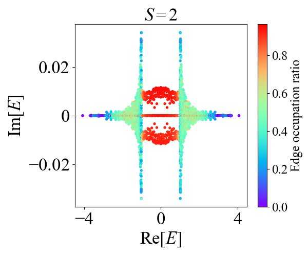
Most saliently, exhibits real-to-complex edge PT breaking as the system width is increased beyond a certain critical (with fixed unit cells), as predicted by Eq. 2 and confirmed in the spectral plots of Fig. 2(a1)-(a4). Here unit cells, as confirmed by detailed dynamical simulations below. Each eigenenergy in Fig. 2(a) is colored according to the edge occupation ratio of its eigenstate , defined as
| (4) |
such that the bulk spectra appear cyan or blue while the edge modes are red. Evidently, edge eigenenergies (red) transition from real to complex as increases, becoming entirely complex by .
To definitively show that this edge PT transition indeed occurs due to topological guided gain mechanism, we simulate the state dynamics in due to a source excitation at , the top left corner of the upper (but not lower) layer. To resonantly excite the topological edge modes [80] and minimize bulk leakage, we simulated the dynamics using the frequency-shifted Hamiltonian , such that lies exactly in the middle of the topological gap. We set and .
Fig. 2(b) showcases the dynamical state evolution to the time-dependent differential equation over one loop , for short and long lattices ( and ), corresponding to the real and complex edge spectra in Figs. 2(a1) and (a4) respectively. For short , the state shrinks as it is chirally transported towards the right in the upper layer and grows back as it loops back, hardly affected by the lower layer, reminiscent of Fig. 1(b). But for long , the state grows simultaneously in both layers in the region , thereby giving rise to net gain, as also foreshadowed in Fig. 1(c).
To more clearly observe that leads to net gain, we plot the numerically obtained total state amplitude over the whole system in Fig. 2(c). For , there is no sustained gain at long times, as expected from the real edge spectra. But for , the empirical topologically guided gain [80]
| (5) |
can be read from the nonzero asymptotic gradient of the log plot. It exhibits close agreement with the growth rate predicted by Eq. 2 (dashed) using the dynamically determined values of the chiral velocity and inverse spatial decay length (with ) [80].
The soundness of our theoretical framework is further verified in Fig. 2(d), where is shown to decrease logarithmically with the interlayer coupling across various non-Hermiticity , exactly consistent with Eq. 1 (dashed) if we set i.e. that the interlayer tunneling and coupling are proportionally related. Here, the data points are empirically obtained as the smallest whereby starts to increase exponentially with time.
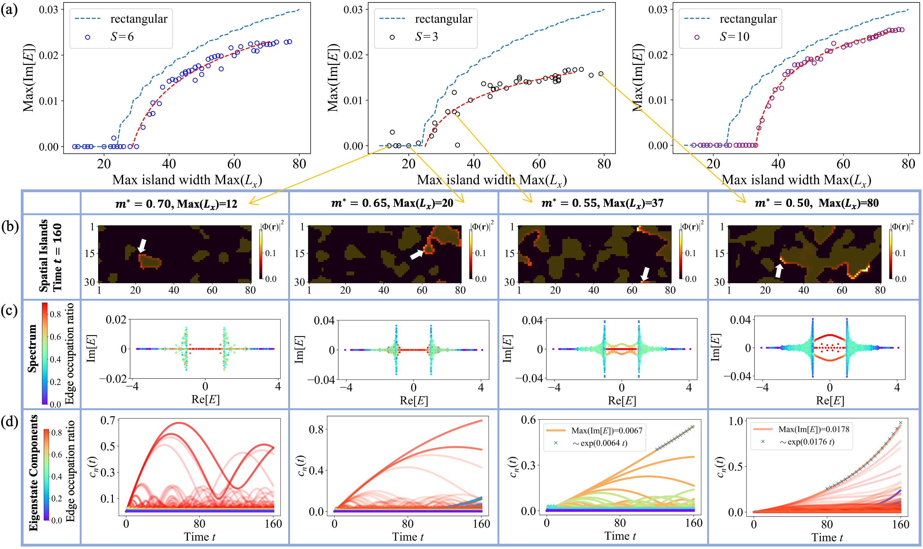
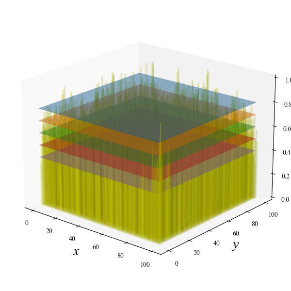
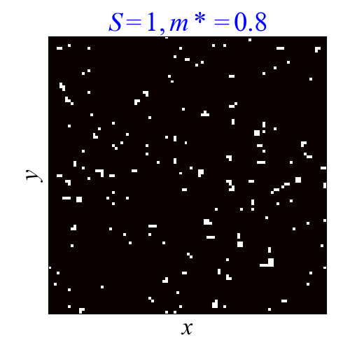
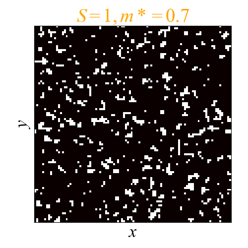
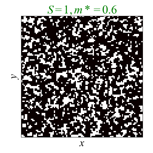
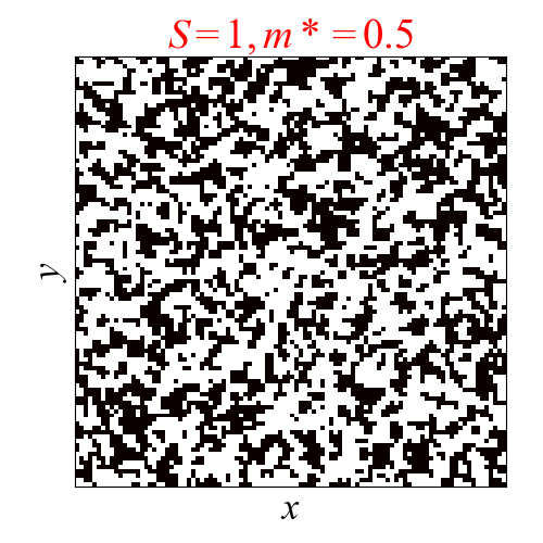
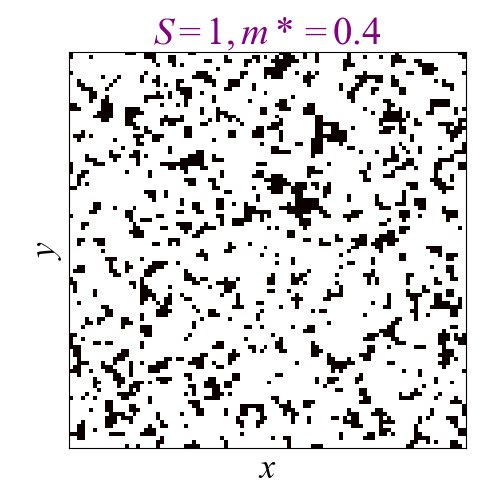
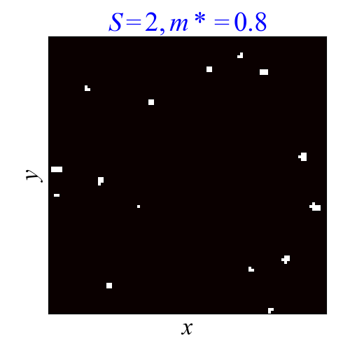
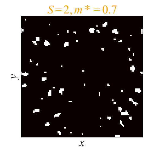
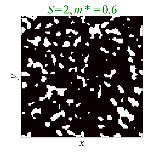
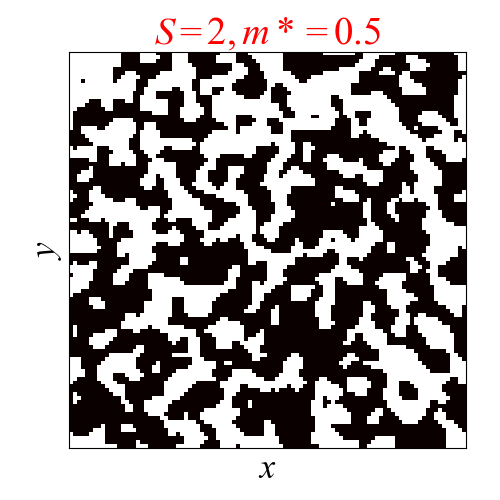
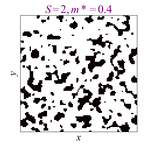
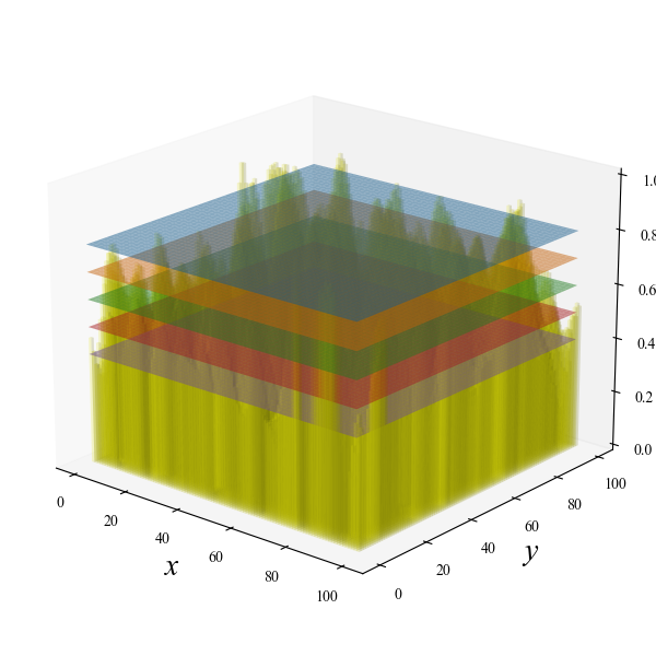
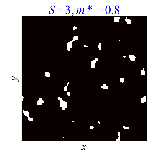
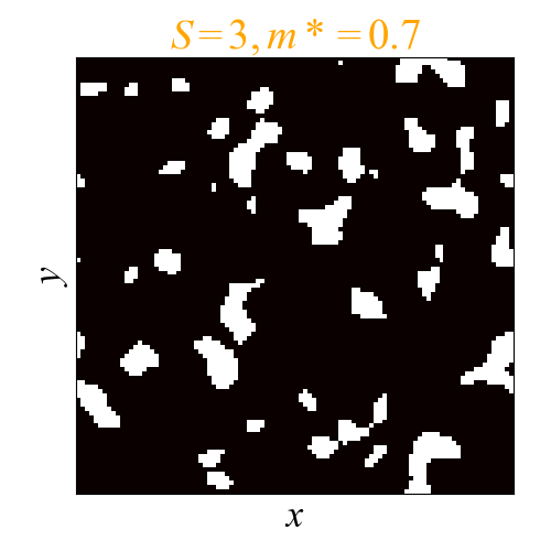
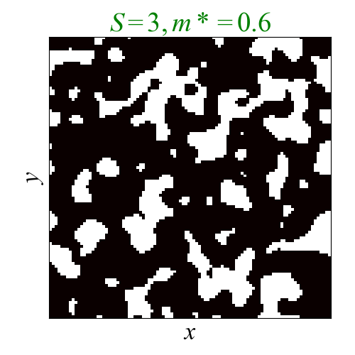
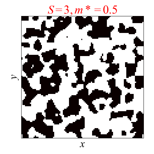
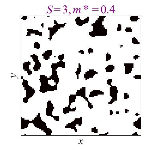
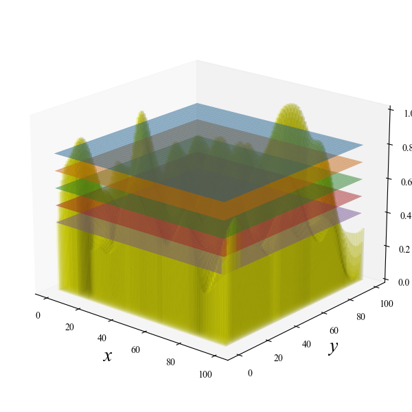
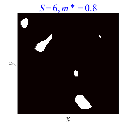
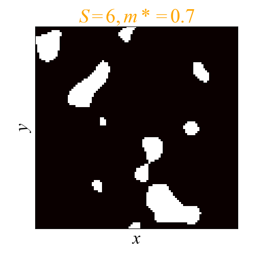
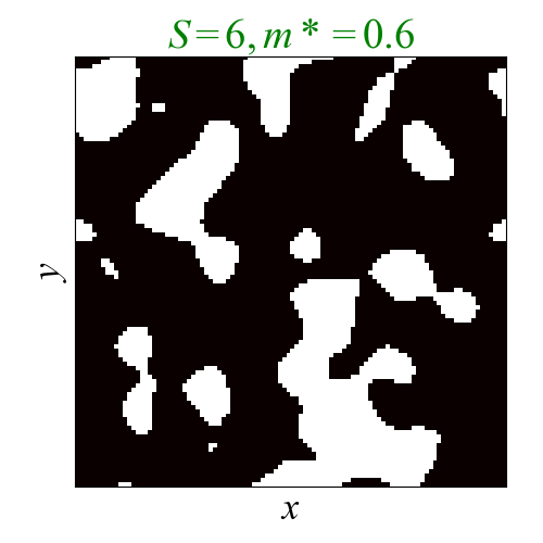
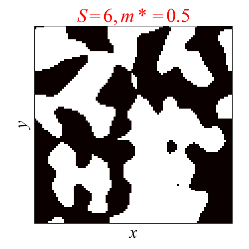
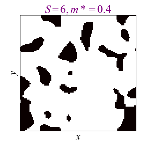
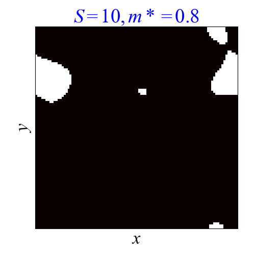
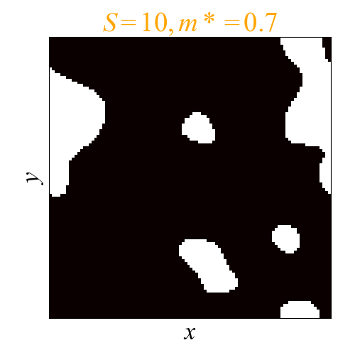
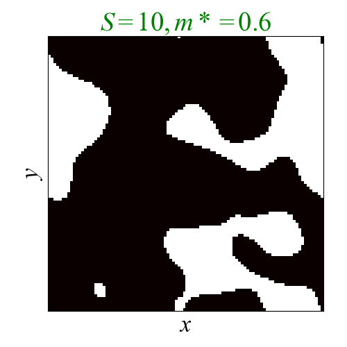
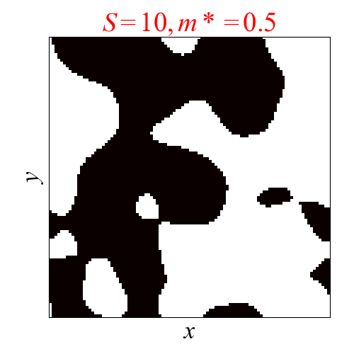
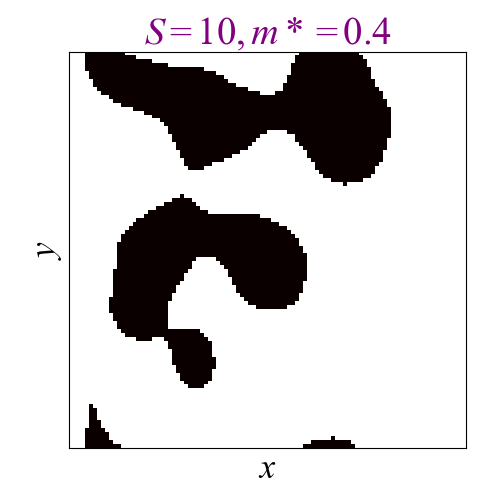
Percolation-induced PT symmetry breaking. – Having established that rectangular islands exhibit edge PT breaking due to topologically guided gain when their width , we next show that this applies also to disordered islands that can dramatically grow via percolation. In this work, percolation is effected by adjusting the “sea level” upon a scalar landscape with random Gaussian correlation , whose generation is detailed in [80]. Regions where are above the “sea level” are designated to be nontrivial topological Chern islands ( in Eq. 3), with boundary smoothness controlled by the correlation length . From previous arguments, the widest island (with width denoted as ) is expected to control the asymptotic state growth. As illustrated in Fig. 3(b) in a periodic -unit cell system with , decreasing the sea level allows the topological islands (white) to grow and coalesce, eventually spanning the entire system as saturates at . How exactly the distribution of the island sizes depends on is described in [80].
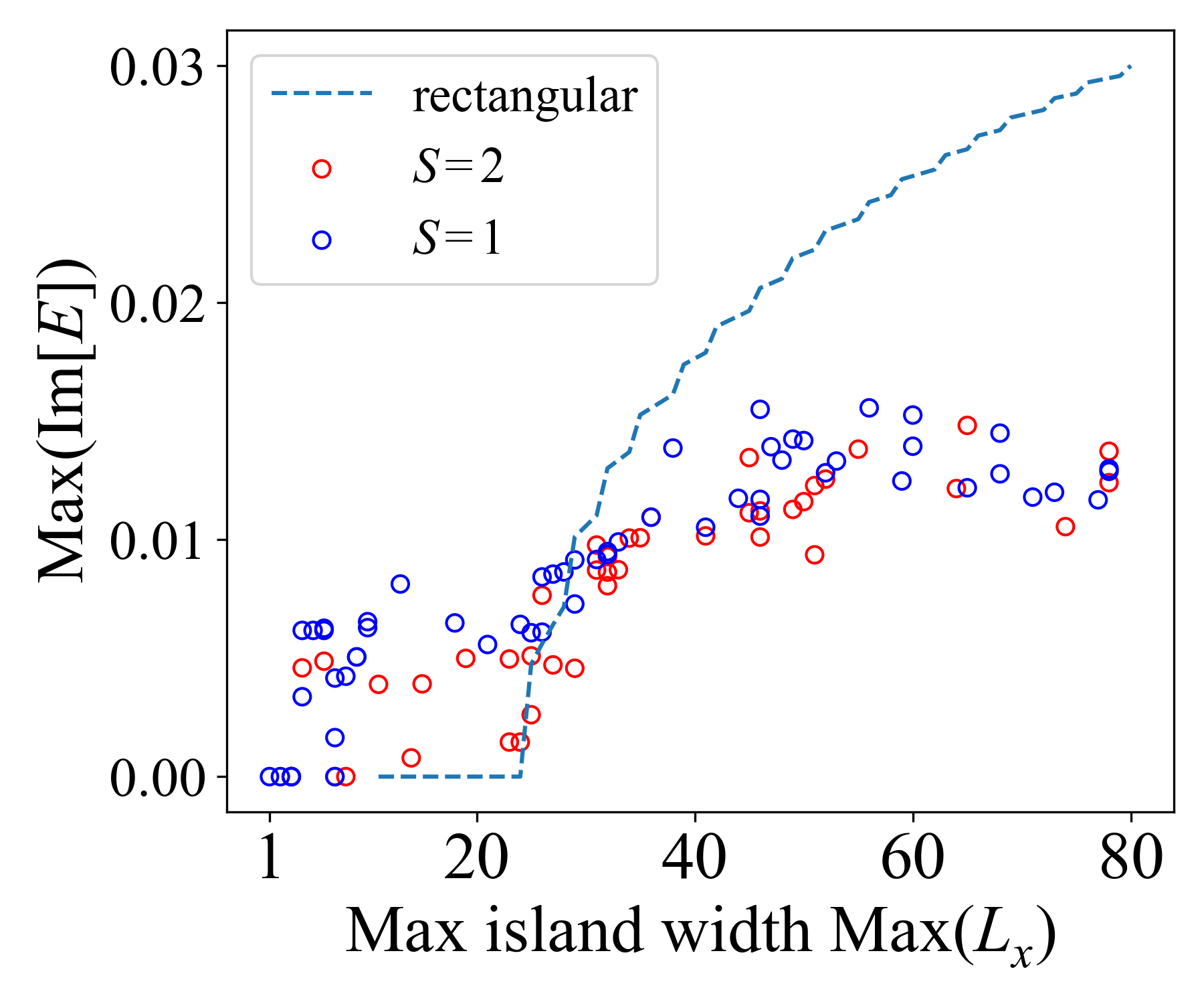
Fig. 3(a) shows the distinctive real-to-complex spectral transition of of the edge modes as the largest island width increases. Whether the island boundaries are rough () or smooth (), we always have when is sufficiently large i.e. where at least one island is wide enough to support topologically guided gain. Crucially in this disordered scenario, the edge dynamics involve a competition between topologically guided propagation/gain and bulk leakage, which can also lead to unlimited growth. While small island features can hinder the gain and lead to lower growth () compared to that in perfectly rectangular islands (blue dashed), they also introduce fluctuations in due to bulk leakage.
Figs. 3(b)-(d) showcases the spectral and corresponding dynamical behavior in four specific disordered instances with , which allows for small island features without excessively sharp boundaries that overshadow the edge PT transition with bulk leakage. For sufficiently large and , the complex edge spectra (red in Figs. 3(c)) can indeed be attributed to the topologically guided gainy propagation around a sufficiently large island, as displayed in Figs. 3(b).
To unambiguously confirm that the numerical state dynamics are indeed governed by obtained from diagonalization, we further plot in Figs. 3(d) the eigenbasis expansion coefficients of the time-evolved state , where ranges over all eigenstates. When as for and , the coefficients oscillate without clear exponential growth; while for the case dominated by a island stretching across the system edges, the leading from the growth of closely matches the growth rate independently obtained from diagonalization. Topologically guided gain can still remain as the primary evolution mechanism in the presence of some bulk leakage (orange or green), such as in the case where the leading growth is still qualitatively predicted by .
Conclusion.– From the triple interplay of chiral topology, directed gain and interlayer tunneling emerges the mechanism of topologically guided gain, where edge wavepackets on sufficiently wide islands experience irreversible growth due to interlayer feedback. We demonstrated this first schematically, then on a single rectangular island, and finally in a disordered landscape of topological islands. For sufficiently smooth islands, a sharp PT symmetry transition occurs as smaller islands percolate and combine to form larger islands beyond a threshold width. Moving forward, it would be interesting to explore how topological guiding can interplay with non-linear feedback [81, 82, 83, 84, 85, 86, 87] and interlayer tunneling subject to Moire interference [88, 89, 90, 91, 92, 93], as well as experimental demonstrations built upon mature mechanical [94, 95, 96, 97], photonic [98, 99, 100, 101, 102], electrical circuit [103, 104, 56, 105, 106, 107, 108, 109, 110, 111, 112, 113, 114, 115] and quantum circuit platforms [116, 117, 118, 119, 120, 121, 122, 123, 124, 125, 126].
References
- Bender and Boettcher [1998] C. M. Bender and S. Boettcher, Real spectra in non-hermitian hamiltonians having p t symmetry, Physical review letters 80, 5243 (1998).
- Bender [2007] C. M. Bender, Making sense of non-hermitian hamiltonians, Reports on Progress in Physics 70, 947 (2007).
- Bender [2023] C. M. Bender, Pt symmetry, in TIME AND SCIENCE: Volume 3: Physical Sciences and Cosmology (World Scientific, 2023) pp. 285–310.
- El-Ganainy et al. [2007] R. El-Ganainy, K. Makris, D. Christodoulides, and Z. H. Musslimani, Theory of coupled optical pt-symmetric structures, Optics letters 32, 2632 (2007).
- Makris et al. [2008] K. G. Makris, R. El-Ganainy, D. Christodoulides, and Z. H. Musslimani, Beam dynamics in p t symmetric optical lattices, Physical Review Letters 100, 103904 (2008).
- Longhi [2009] S. Longhi, Bloch oscillations in complex crystals with p t symmetry, Physical review letters 103, 123601 (2009).
- Bendix et al. [2009] O. Bendix, R. Fleischmann, T. Kottos, and B. Shapiro, Exponentially fragile p t symmetry in lattices with localized eigenmodes, Physical Review Letters 103, 030402 (2009).
- Rüter et al. [2010] C. E. Rüter, K. G. Makris, R. El-Ganainy, D. N. Christodoulides, M. Segev, and D. Kip, Observation of parity–time symmetry in optics, Nature physics 6, 192 (2010).
- Lin et al. [2011] Z. Lin, H. Ramezani, T. Eichelkraut, T. Kottos, H. Cao, and D. N. Christodoulides, Unidirectional invisibility induced by p t-symmetric periodic structures, Physical Review Letters 106, 213901 (2011).
- Schindler et al. [2011] J. Schindler, A. Li, M. C. Zheng, F. M. Ellis, and T. Kottos, Experimental study of active lrc circuits with pt symmetries, Physical Review A 84, 040101 (2011).
- Mostafazadeh [2013] A. Mostafazadeh, Invisibility and pt symmetry, Physical Review A 87, 012103 (2013).
- Zhu et al. [2013] X. Zhu, L. Feng, P. Zhang, X. Yin, and X. Zhang, One-way invisible cloak using parity-time symmetric transformation optics, Optics letters 38, 2821 (2013).
- Zyablovsky et al. [2014] A. A. Zyablovsky, A. P. Vinogradov, A. A. Pukhov, A. V. Dorofeenko, and A. A. Lisyansky, Pt-symmetry in optics, Physics-Uspekhi 57, 1063 (2014).
- Chang et al. [2014] L. Chang, X. Jiang, S. Hua, C. Yang, J. Wen, L. Jiang, G. Li, G. Wang, and M. Xiao, Parity–time symmetry and variable optical isolation in active–passive-coupled microresonators, Nature photonics 8, 524 (2014).
- Sounas et al. [2015] D. L. Sounas, R. Fleury, and A. Alù, Unidirectional cloaking based on metasurfaces with balanced loss and gain, Physical Review Applied 4, 014005 (2015).
- Konotop et al. [2016] V. V. Konotop, J. Yang, and D. A. Zezyulin, Nonlinear waves in pt-symmetric systems, Reviews of Modern Physics 88, 035002 (2016).
- Liu et al. [2016] Z.-P. Liu, J. Zhang, Ş. K. Özdemir, B. Peng, H. Jing, X.-Y. Lü, C.-W. Li, L. Yang, F. Nori, and Y.-x. Liu, Metrology with pt-symmetric cavities: enhanced sensitivity near the pt-phase transition, Physical review letters 117, 110802 (2016).
- Assawaworrarit et al. [2017] S. Assawaworrarit, X. Yu, and S. Fan, Robust wireless power transfer using a nonlinear parity–time-symmetric circuit, Nature 546, 387 (2017).
- El-Ganainy et al. [2018] R. El-Ganainy, K. G. Makris, M. Khajavikhan, Z. H. Musslimani, S. Rotter, and D. N. Christodoulides, Non-hermitian physics and pt symmetry, Nature Physics 14, 11 (2018).
- Chen et al. [2018] P.-Y. Chen, M. Sakhdari, M. Hajizadegan, Q. Cui, M. M.-C. Cheng, R. El-Ganainy, and A. Alù, Generalized parity–time symmetry condition for enhanced sensor telemetry, Nature Electronics 1, 297 (2018).
- Lee [2022] C. H. Lee, Exceptional bound states and negative entanglement entropy, Physical Review Letters 128, 010402 (2022).
- Liu et al. [2018] Y. Liu, T. Hao, W. Li, J. Capmany, N. Zhu, and M. Li, Observation of parity-time symmetry in microwave photonics, Light: Science & Applications 7, 38 (2018).
- Özdemir et al. [2019] Ş. K. Özdemir, S. Rotter, F. Nori, and L. Yang, Parity–time symmetry and exceptional points in photonics, Nature materials 18, 783 (2019).
- Shao et al. [2020] L. Shao, W. Mao, S. Maity, N. Sinclair, Y. Hu, L. Yang, and M. Lončar, Non-reciprocal transmission of microwave acoustic waves in nonlinear parity–time symmetric resonators, Nature Electronics 3, 267 (2020).
- Stauffer [1979] D. Stauffer, Scaling theory of percolation clusters, Physics reports 54, 1 (1979).
- Essam [1980] J. W. Essam, Percolation theory, Reports on progress in physics 43, 833 (1980).
- Hu [1984] C.-K. Hu, Percolation, clusters, and phase transitions in spin models, Physical Review B 29, 5103 (1984).
- Parshani et al. [2010] R. Parshani, S. V. Buldyrev, and S. Havlin, Interdependent networks: Reducing the coupling strength leads to a change from a first to second order percolation transition, Physical review letters 105, 048701 (2010).
- Lemoult et al. [2016] G. Lemoult, L. Shi, K. Avila, S. V. Jalikop, M. Avila, and B. Hof, Directed percolation phase transition to sustained turbulence in couette flow, Nature Physics 12, 254 (2016).
- Cardy [1992] J. L. Cardy, Critical percolation in finite geometries, Journal of Physics A: Mathematical and General 25, L201 (1992).
- Mathieu and Ridout [2007] P. Mathieu and D. Ridout, From percolation to logarithmic conformal field theory, Physics Letters B 657, 120 (2007).
- Mertens and Moore [2012] S. Mertens and C. Moore, Continuum percolation thresholds in two dimensions, Physical Review E 86, 061109 (2012).
- Li et al. [2007] J. Li, P. C. Ma, W. S. Chow, C. K. To, B. Z. Tang, and J.-K. Kim, Correlations between percolation threshold, dispersion state, and aspect ratio of carbon nanotubes, Advanced Functional Materials 17, 3207 (2007).
- Mavko and Nur [1997] G. Mavko and A. Nur, The effect of a percolation threshold in the kozeny-carman relation, Geophysics 62, 1480 (1997).
- Coniglio [1982] A. Coniglio, Cluster structure near the percolation threshold, Journal of Physics A: Mathematical and General 15, 3829 (1982).
- Balberg et al. [1984] I. Balberg, N. Binenbaum, and N. Wagner, Percolation thresholds in the three-dimensional sticks system, Physical Review Letters 52, 1465 (1984).
- Hinrichsen [2000] H. Hinrichsen, Non-equilibrium critical phenomena and phase transitions into absorbing states, Advances in physics 49, 815 (2000).
- Goltsev et al. [2006] A. V. Goltsev, S. N. Dorogovtsev, and J. F. F. Mendes, k-core (bootstrap) percolation on complex networks: Critical phenomena and nonlocal effects, Physical Review E 73, 056101 (2006).
- Dorogovtsev et al. [2008] S. N. Dorogovtsev, A. V. Goltsev, and J. F. Mendes, Critical phenomena in complex networks, Reviews of Modern Physics 80, 1275 (2008).
- Shante and Kirkpatrick [1971] V. K. Shante and S. Kirkpatrick, An introduction to percolation theory, Advances in Physics 20, 325 (1971).
- Kirkpatrick [1973] S. Kirkpatrick, Percolation and conduction, Reviews of modern physics 45, 574 (1973).
- Bollobás and Riordan [2006] B. Bollobás and O. Riordan, Percolation (Cambridge University Press, 2006).
- Saberi [2015] A. A. Saberi, Recent advances in percolation theory and its applications, Physics Reports 578, 1 (2015).
- Lee [2016] T. E. Lee, Anomalous edge state in a non-hermitian lattice, Physical review letters 116, 133903 (2016).
- Alvarez et al. [2018] V. M. Alvarez, J. B. Vargas, and L. F. Torres, Non-hermitian robust edge states in one dimension: Anomalous localization and eigenspace condensation at exceptional points, Physical Review B 97, 121401 (2018).
- Yao and Wang [2018] S. Yao and Z. Wang, Edge states and topological invariants of non-hermitian systems, Physical review letters 121, 086803 (2018).
- Kunst et al. [2018] F. K. Kunst, E. Edvardsson, J. C. Budich, and E. J. Bergholtz, Biorthogonal bulk-boundary correspondence in non-hermitian systems, Physical review letters 121, 026808 (2018).
- Lee and Thomale [2019] C. H. Lee and R. Thomale, Anatomy of skin modes and topology in non-hermitian systems, Physical Review B 99, 201103 (2019).
- Okuma et al. [2020] N. Okuma, K. Kawabata, K. Shiozaki, and M. Sato, Topological origin of non-hermitian skin effects, Physical review letters 124, 086801 (2020).
- Lin et al. [2023] R. Lin, T. Tai, L. Li, and C. H. Lee, Topological non-hermitian skin effect, Frontiers of Physics 18, 53605 (2023).
- Okuma and Sato [2023] N. Okuma and M. Sato, Non-hermitian topological phenomena: A review, Annual Review of Condensed Matter Physics 14, 83 (2023).
- Longhi [2019] S. Longhi, Topological phase transition in non-hermitian quasicrystals, Physical review letters 122, 237601 (2019).
- Kawabata et al. [2019] K. Kawabata, K. Shiozaki, M. Ueda, and M. Sato, Symmetry and topology in non-hermitian physics, Physical Review X 9, 041015 (2019).
- Lee et al. [2019] C. H. Lee, L. Li, and J. Gong, Hybrid higher-order skin-topological modes in nonreciprocal systems, Physical review letters 123, 016805 (2019).
- Song et al. [2019] F. Song, S. Yao, and Z. Wang, Non-hermitian skin effect and chiral damping in open quantum systems, Physical review letters 123, 170401 (2019).
- Helbig et al. [2020] T. Helbig, T. Hofmann, S. Imhof, M. Abdelghany, T. Kiessling, L. Molenkamp, C. Lee, A. Szameit, M. Greiter, and R. Thomale, Generalized bulk–boundary correspondence in non-hermitian topolectrical circuits, Nature Physics 16, 747 (2020).
- Li et al. [2020] L. Li, C. H. Lee, S. Mu, and J. Gong, Critical non-hermitian skin effect, Nature communications 11, 5491 (2020).
- Xue et al. [2022] W.-T. Xue, Y.-M. Hu, F. Song, and Z. Wang, Non-hermitian edge burst, Physical Review Letters 128, 120401 (2022).
- Lee et al. [2020] C. H. Lee, L. Li, R. Thomale, and J. Gong, Unraveling non-hermitian pumping: emergent spectral singularities and anomalous responses, Physical Review B 102, 085151 (2020).
- Zou et al. [2021] D. Zou, T. Chen, W. He, J. Bao, C. H. Lee, H. Sun, and X. Zhang, Observation of hybrid higher-order skin-topological effect in non-hermitian topolectrical circuits, Nature Communications 12, 7201 (2021).
- Zhang et al. [2021] X. Zhang, Y. Tian, J.-H. Jiang, M.-H. Lu, and Y.-F. Chen, Observation of higher-order non-hermitian skin effect, Nature communications 12, 5377 (2021).
- Yang et al. [2022] M. Yang, L. Wang, X. Wu, H. Xiao, D. Yu, L. Yuan, and X. Chen, Concentrated subradiant modes in a one-dimensional atomic array coupled with chiral waveguides, Physical Review A 106, 043717 (2022).
- Li and Lee [2022] L. Li and C. H. Lee, Non-hermitian pseudo-gaps, Science Bulletin 67, 685 (2022).
- Longhi [2022] S. Longhi, Self-healing of non-hermitian topological skin modes, Physical Review Letters 128, 157601 (2022).
- Gu et al. [2022] Z. Gu, H. Gao, H. Xue, J. Li, Z. Su, and J. Zhu, Transient non-hermitian skin effect, Nature Communications 13, 7668 (2022).
- Shen and Lee [2022] R. Shen and C. H. Lee, Non-hermitian skin clusters from strong interactions, Communications Physics 5, 238 (2022).
- Jiang and Lee [2023] H. Jiang and C. H. Lee, Dimensional transmutation from non-hermiticity, Physical Review Letters 131, 076401 (2023).
- Tai and Lee [2023] T. Tai and C. H. Lee, Zoology of non-hermitian spectra and their graph topology, Physical Review B 107, L220301 (2023).
- Longhi [2020] S. Longhi, Non-bloch-band collapse and chiral zener tunneling, Physical review letters 124, 066602 (2020).
- Bernevig [2013] B. A. Bernevig, Topological insulators and topological superconductors (Princeton university press, 2013).
- Qi and Zhang [2011] X.-L. Qi and S.-C. Zhang, Topological insulators and superconductors, Reviews of Modern Physics 83, 1057 (2011).
- Hasan and Kane [2010] M. Z. Hasan and C. L. Kane, Colloquium: topological insulators, Reviews of modern physics 82, 3045 (2010).
- Asbóth et al. [2016] J. K. Asbóth, L. Oroszlány, and A. Pályi, A short course on topological insulators, Lecture notes in physics 919, 166 (2016).
- Note [1] But still with much smaller than the topological gap.
- Liu et al. [2020a] C.-H. Liu, K. Zhang, Z. Yang, and S. Chen, Helical damping and dynamical critical skin effect in open quantum systems, Physical Review Research 2, 043167 (2020a).
- Yokomizo and Murakami [2021] K. Yokomizo and S. Murakami, Scaling rule for the critical non-hermitian skin effect, Physical Review B 104, 165117 (2021).
- Qin et al. [2023] F. Qin, Y. Ma, R. Shen, C. H. Lee, et al., Universal competitive spectral scaling from the critical non-hermitian skin effect, Physical Review B 107, 155430 (2023).
- Qi et al. [2006] X.-L. Qi, Y.-S. Wu, and S.-C. Zhang, Topological quantization of the spin hall effect in two-dimensional paramagnetic semiconductors, Physical Review B 74, 085308 (2006).
- Kawabata et al. [2018] K. Kawabata, K. Shiozaki, and M. Ueda, Anomalous helical edge states in a non-hermitian chern insulator, Phys. Rev. B 98, 165148 (2018).
- [80] See supplemental material.
- Zhou et al. [2017] X. Zhou, Y. Wang, D. Leykam, and Y. D. Chong, Optical isolation with nonlinear topological photonics, New Journal of Physics 19, 095002 (2017).
- Smirnova et al. [2019] D. A. Smirnova, L. A. Smirnov, D. Leykam, and Y. S. Kivshar, Topological edge states and gap solitons in the nonlinear dirac model, Laser & Photonics Reviews 13, 1900223 (2019).
- Tuloup et al. [2020] T. Tuloup, R. W. Bomantara, C. H. Lee, and J. Gong, Nonlinearity induced topological physics in momentum space and real space, Physical Review B 102, 115411 (2020).
- Smirnova et al. [2020] D. Smirnova, D. Leykam, Y. Chong, and Y. Kivshar, Nonlinear topological photonics, Applied Physics Reviews 7 (2020).
- Xia et al. [2021] S. Xia, D. Kaltsas, D. Song, I. Komis, J. Xu, A. Szameit, H. Buljan, K. G. Makris, and Z. Chen, Nonlinear tuning of pt symmetry and non-hermitian topological states, Science 372, 72 (2021).
- Sone et al. [2022] K. Sone, Y. Ashida, and T. Sagawa, Topological synchronization of coupled nonlinear oscillators, Physical Review Research 4, 023211 (2022).
- Hohmann et al. [2023] H. Hohmann, T. Hofmann, T. Helbig, S. Imhof, H. Brand, L. K. Upreti, A. Stegmaier, A. Fritzsche, T. Müller, U. Schwingenschlögl, et al., Observation of cnoidal wave localization in nonlinear topolectric circuits, Physical Review Research 5, L012041 (2023).
- Ohta et al. [2012] T. Ohta, J. T. Robinson, P. J. Feibelman, A. Bostwick, E. Rotenberg, and T. E. Beechem, Evidence for interlayer coupling and moiré periodic potentials in twisted bilayer graphene, Physical Review Letters 109, 186807 (2012).
- Dai et al. [2016] S. Dai, Y. Xiang, and D. J. Srolovitz, Twisted bilayer graphene: Moiré with a twist, Nano letters 16, 5923 (2016).
- Kim et al. [2017] K. Kim, A. DaSilva, S. Huang, B. Fallahazad, S. Larentis, T. Taniguchi, K. Watanabe, B. J. LeRoy, A. H. MacDonald, and E. Tutuc, Tunable moiré bands and strong correlations in small-twist-angle bilayer graphene, Proceedings of the National Academy of Sciences 114, 3364 (2017).
- Naik and Jain [2018] M. H. Naik and M. Jain, Ultraflatbands and shear solitons in moiré patterns of twisted bilayer transition metal dichalcogenides, Physical review letters 121, 266401 (2018).
- Carr et al. [2020] S. Carr, S. Fang, and E. Kaxiras, Electronic-structure methods for twisted moiré layers, Nature Reviews Materials 5, 748 (2020).
- de Jong et al. [2022] T. A. de Jong, T. Benschop, X. Chen, E. E. Krasovskii, M. J. de Dood, R. M. Tromp, M. P. Allan, and S. J. Van der Molen, Imaging moiré deformation and dynamics in twisted bilayer graphene, Nature Communications 13, 70 (2022).
- Brandenbourger et al. [2019] M. Brandenbourger, X. Locsin, E. Lerner, and C. Coulais, Non-reciprocal robotic metamaterials, Nature communications 10, 4608 (2019).
- Ghatak et al. [2020] A. Ghatak, M. Brandenbourger, J. Van Wezel, and C. Coulais, Observation of non-hermitian topology and its bulk–edge correspondence in an active mechanical metamaterial, Proceedings of the National Academy of Sciences 117, 29561 (2020).
- Wen et al. [2022] X. Wen, X. Zhu, A. Fan, W. Y. Tam, J. Zhu, H. W. Wu, F. Lemoult, M. Fink, and J. Li, Unidirectional amplification with acoustic non-hermitian space- time varying metamaterial, Communications physics 5, 18 (2022).
- Xiu et al. [2023] H. Xiu, I. Frankel, H. Liu, K. Qian, S. Sarkar, B. MacNider, Z. Chen, N. Boechler, and X. Mao, Synthetically non-hermitian nonlinear wave-like behavior in a topological mechanical metamaterial, Proceedings of the National Academy of Sciences 120, e2217928120 (2023).
- Pan et al. [2018] M. Pan, H. Zhao, P. Miao, S. Longhi, and L. Feng, Photonic zero mode in a non-hermitian photonic lattice, Nature communications 9, 1308 (2018).
- Xiao et al. [2020] L. Xiao, T. Deng, K. Wang, G. Zhu, Z. Wang, W. Yi, and P. Xue, Non-hermitian bulk–boundary correspondence in quantum dynamics, Nature Physics 16, 761 (2020).
- Zhu et al. [2020] X. Zhu, H. Wang, S. K. Gupta, H. Zhang, B. Xie, M. Lu, and Y. Chen, Photonic non-hermitian skin effect and non-bloch bulk-boundary correspondence, Physical Review Research 2, 013280 (2020).
- Song et al. [2020] Y. Song, W. Liu, L. Zheng, Y. Zhang, B. Wang, and P. Lu, Two-dimensional non-hermitian skin effect in a synthetic photonic lattice, Physical Review Applied 14, 064076 (2020).
- Ao et al. [2020] Y. Ao, X. Hu, Y. You, C. Lu, Y. Fu, X. Wang, and Q. Gong, Topological phase transition in the non-hermitian coupled resonator array, Physical Review Letters 125, 013902 (2020).
- Hofmann et al. [2019] T. Hofmann, T. Helbig, C. H. Lee, M. Greiter, and R. Thomale, Chiral voltage propagation and calibration in a topolectrical chern circuit, Physical review letters 122, 247702 (2019).
- Ezawa [2019] M. Ezawa, Electric circuits for non-hermitian chern insulators, Physical Review B 100, 081401 (2019).
- Hofmann et al. [2020] T. Hofmann, T. Helbig, F. Schindler, N. Salgo, M. Brzezińska, M. Greiter, T. Kiessling, D. Wolf, A. Vollhardt, A. Kabaši, et al., Reciprocal skin effect and its realization in a topolectrical circuit, Physical Review Research 2, 023265 (2020).
- Liu et al. [2020b] S. Liu, S. Ma, C. Yang, L. Zhang, W. Gao, Y. J. Xiang, T. J. Cui, and S. Zhang, Gain-and loss-induced topological insulating phase in a non-hermitian electrical circuit, Physical Review Applied 13, 014047 (2020b).
- Liu et al. [2021] S. Liu, R. Shao, S. Ma, L. Zhang, O. You, H. Wu, Y. J. Xiang, T. J. Cui, and S. Zhang, Non-hermitian skin effect in a non-hermitian electrical circuit, Research (2021).
- Stegmaier et al. [2021] A. Stegmaier, S. Imhof, T. Helbig, T. Hofmann, C. H. Lee, M. Kremer, A. Fritzsche, T. Feichtner, S. Klembt, S. Höfling, et al., Topological defect engineering and p t symmetry in non-hermitian electrical circuits, Physical Review Letters 126, 215302 (2021).
- Zhang and Franz [2020] X.-X. Zhang and M. Franz, Non-hermitian exceptional landau quantization in electric circuits, Physical Review Letters 124, 046401 (2020).
- Zhang et al. [2022] X. Zhang, B. Zhang, W. Zhao, and C. H. Lee, Observation of non-local impedance response in a passive electrical circuit, arXiv preprint arXiv:2211.09152 (2022).
- Shang et al. [2022] C. Shang, S. Liu, R. Shao, P. Han, X. Zang, X. Zhang, K. N. Salama, W. Gao, C. H. Lee, R. Thomale, et al., Experimental identification of the second-order non-hermitian skin effect with physics-graph-informed machine learning, Advanced Science 9, 2202922 (2022).
- Yuan et al. [2023] H. Yuan, W. Zhang, Z. Zhou, W. Wang, N. Pan, Y. Feng, H. Sun, and X. Zhang, Non-hermitian topolectrical circuit sensor with high sensitivity, Advanced Science , 2301128 (2023).
- Zou et al. [2023] D. Zou, T. Chen, H. Meng, Y. S. Ang, X. Zhang, and C. H. Lee, Experimental observation of exceptional bound states in a classical circuit network, arXiv preprint arXiv:2308.01970 (2023).
- Zhu et al. [2023] P. Zhu, X.-Q. Sun, T. L. Hughes, and G. Bahl, Higher rank chirality and non-hermitian skin effect in a topolectrical circuit, Nature communications 14, 720 (2023).
- Zhang et al. [2023] H. Zhang, T. Chen, L. Li, C. H. Lee, and X. Zhang, Electrical circuit realization of topological switching for the non-hermitian skin effect, Physical Review B 107, 085426 (2023).
- Smith et al. [2019] A. Smith, M. Kim, F. Pollmann, and J. Knolle, Simulating quantum many-body dynamics on a current digital quantum computer, npj Quantum Information 5, 106 (2019).
- Gou et al. [2020] W. Gou, T. Chen, D. Xie, T. Xiao, T.-S. Deng, B. Gadway, W. Yi, and B. Yan, Tunable nonreciprocal quantum transport through a dissipative aharonov-bohm ring in ultracold atoms, Physical review letters 124, 070402 (2020).
- Koh et al. [2022] J. M. Koh, T. Tai, and C. H. Lee, Simulation of interaction-induced chiral topological dynamics on a digital quantum computer, Physical Review Letters 129, 140502 (2022).
- Kirmani et al. [2022] A. Kirmani, K. Bull, C.-Y. Hou, V. Saravanan, S. M. Saeed, Z. Papić, A. Rahmani, and P. Ghaemi, Probing geometric excitations of fractional quantum hall states on quantum computers, Physical Review Letters 129, 056801 (2022).
- Frey and Rachel [2022] P. Frey and S. Rachel, Realization of a discrete time crystal on 57 qubits of a quantum computer, Science advances 8, eabm7652 (2022).
- Chertkov et al. [2023] E. Chertkov, Z. Cheng, A. C. Potter, S. Gopalakrishnan, T. M. Gatterman, J. A. Gerber, K. Gilmore, D. Gresh, A. Hall, A. Hankin, et al., Characterizing a non-equilibrium phase transition on a quantum computer, Nature Physics , 1 (2023).
- Chen et al. [2023] T. Chen, R. Shen, C. H. Lee, B. Yang, and R. W. Bomantara, A robust large-period discrete time crystal and its signature in a digital quantum computer, arXiv preprint arXiv:2309.11560 (2023).
- Yang et al. [2023] Y. Yang, A. Christianen, S. Coll-Vinent, V. Smelyanskiy, M. C. Bañuls, T. E. O’Brien, D. S. Wild, and J. I. Cirac, Simulating prethermalization using near-term quantum computers, PRX Quantum 4, 030320 (2023).
- Iqbal et al. [2023] M. Iqbal, N. Tantivasadakarn, R. Verresen, S. L. Campbell, J. M. Dreiling, C. Figgatt, J. P. Gaebler, J. Johansen, M. Mills, S. A. Moses, et al., Creation of non-abelian topological order and anyons on a trapped-ion processor, arXiv preprint arXiv:2305.03766 (2023).
- Shen et al. [2023] R. Shen, T. Chen, B. Yang, and C. H. Lee, Observation of the non-hermitian skin effect and fermi skin on a digital quantum computer, arXiv preprint arXiv:2311.10143 (2023).
- Koh et al. [2023] J. M. Koh, T. Tai, and C. H. Lee, Observation of higher-order topological states on a quantum computer, arXiv preprint arXiv:2303.02179 (2023).
- Yokomizo and Murakami [2019] K. Yokomizo and S. Murakami, Non-bloch band theory of non-hermitian systems, Physical review letters 123, 066404 (2019).
- Yang et al. [2020] Z. Yang, K. Zhang, C. Fang, and J. Hu, Non-hermitian bulk-boundary correspondence and auxiliary generalized brillouin zone theory, Physical Review Letters 125, 226402 (2020).
- Ong and Lee [2016] Z.-Y. Ong and C. H. Lee, Transport and localization in a topological phononic lattice with correlated disorder, Phys. Rev. B 94, 134203 (2016).
Supplemental Material for “Percolation-induced PT symmetry breaking”
S1 Detailed analysis of the dynamical driving term
In the main text, we have used the fact that the driving term does not affect the state growth rate much when the system is in the exponential growth regime, despite still functioning as an energy source. Here we provide a detailed analysis.
The Schrödinger equation for the state evolution subject to a driving term is
| (S1) |
where is the Hamiltonian that is frequency-shifted such that the midgap edge mode correspond to nonzero frequency . Its general solution is given by
| (S2) |
is the time-evolution operator that propagates the undriven state from time to time . But with external driving , the second term (driving term) in Eq. S2 represents the contribution of the external driving throughout the time interval, whose impact is what we are studying. Indeed, the driving term can be thought of as “continually” feeding in a new initial state from to . To proceed, we perform the spectral decomposition of the time-evolution operator , which is given by
| (S3) |
where and are the eigenvalues and eigenvectors of the Hamiltonian . Since may be complex for non-Hermitian Hamiltonians, we rewrite the eigenvalues as
| (S4) |
where is the oscillation frequency and represents growth/decay (positive/negative). The time evolution operator in Eq. S3 then can be rewritten as
| (S5) |
Plugging Eq. S5 into the second term in the integral Eq. S2, we obtain
| (S6) | ||||
The time integral can be evaluated as
| (S7) |
From this, we obtain the contribution of the external driving over the time interval as
| (S8) |
where and as previously defined. This result in Eq. S8 can be explained as follows. represents the coupling strength between the driving field and the -th eigenstate of the system. The driving term excites the eigenstates of the time-evolution operator that have a nonzero overlap with the spatial profile of the driving term, i.e., . This means that the driving term can selectively excite certain eigenstates, depending on the position of the driving source. In the main text, we choose to be at the left-top corner of the rectangular lattice. This position is chosen because the topological edge state is extensively localized there. Therefore, the driving term can effectively and selectively excite the topological edge state as intended.
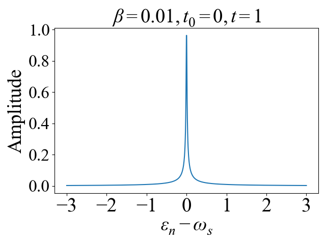
The contribution from the overlap is given by the complex factor that depends on the growth rate , the energy difference , for a time interval . This factor determines the amplitude and phase of the contribution of the -th eigenstate to the final state of the system. The absolute value of the complex factor is given by
| (S9) |
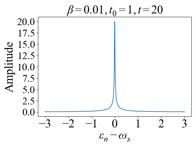
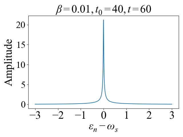
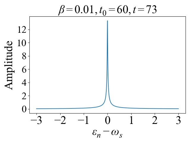
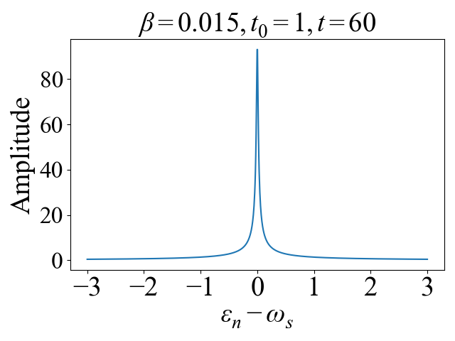
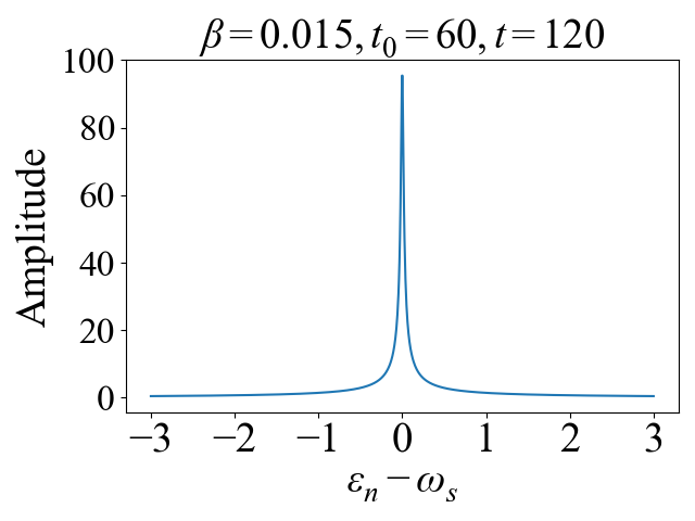
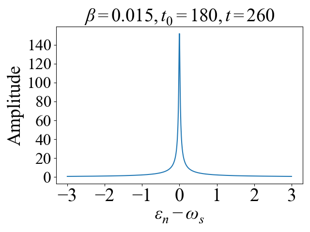
Evidently, for a real eigenenergy (such as a PT-unbroken topological edge mode), and the overwhelming large contribution occurs at resonance . For nonzero , this contribution grows exponentially, as would an overlap contribution with any initial state. However, at small linewidth , a broadened resonance peak around still exists, as illustrated in Figs. S1 and S2. In the text, we used an that resonates with midgap topological edge states with zero or very small before PT breaking.


S2 Estimation of the effective parameters characterizing the dynamically generated edge states
S2.1 Estimation of the decay length for dynamically generated edge states
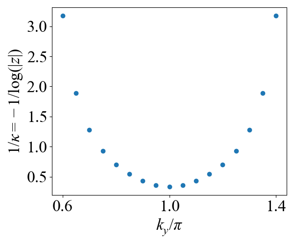
In our topologically guided gain mechanism, the inverse state decay length (inverse skin depth) is the key measure of the asymmetric directionality of the non-Hermitian couplings. We first describe it for our bilayer non-Hermitian Chern model and then show how we can estimate the effective for the dynamically evolved state, which is a superposition of many such modes.
Since the asymmetry is in the -direction, we consider -open boundary conditions (OBCs), such that we obtain effective 1D chains with energy dispersion
| (S10) |
where . We rewrite this as
| (S11) |
such that solutions satisfying are constrained [48, 46, 127, 128, 59] to the OBC energies and satisfy
| (S12) |
such that is given by
| (S13) |
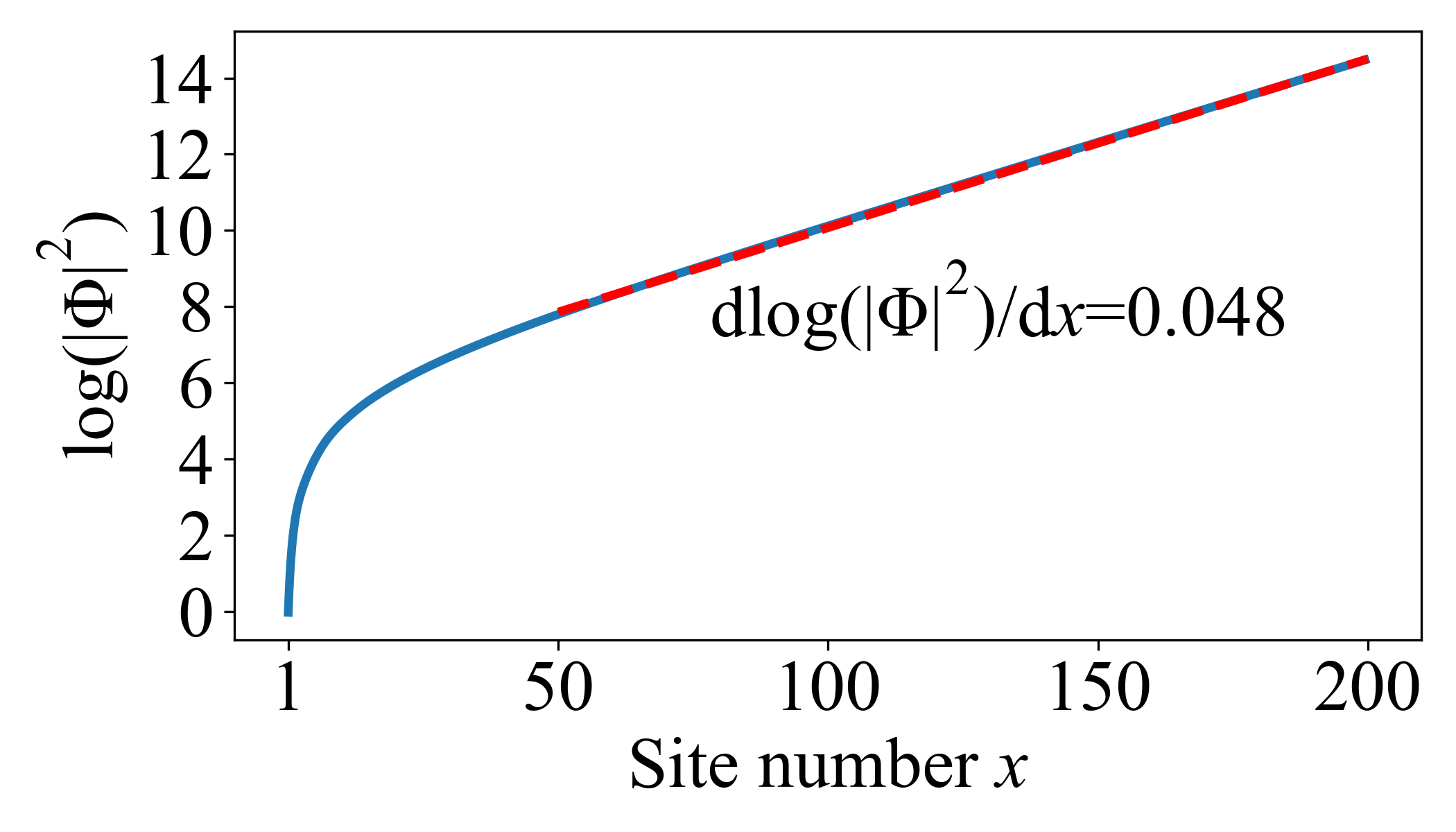
However, in the system where we dynamically excite many modes with different real and imaginary parts of eigenenergies which may correspond to different decay lengths, the decay length is not well defined. In this case, we can define the decay length as the average of the decay length of all the excited modes, corresponding to an effective and corresponding effective .
To empirically obtain the spatial decay rate of the evolved state which was excited by the source , we plot the logarithmic amplitude squared of versus site number, as shown in Fig. S3. The red dashed line is plotted with the slope being 0.048, which should correspond to . As such, we obtain the effective averaged which corresponds to an effective .
S2.2 Estimation of the wavepacket velocity for dynamically generated edge states
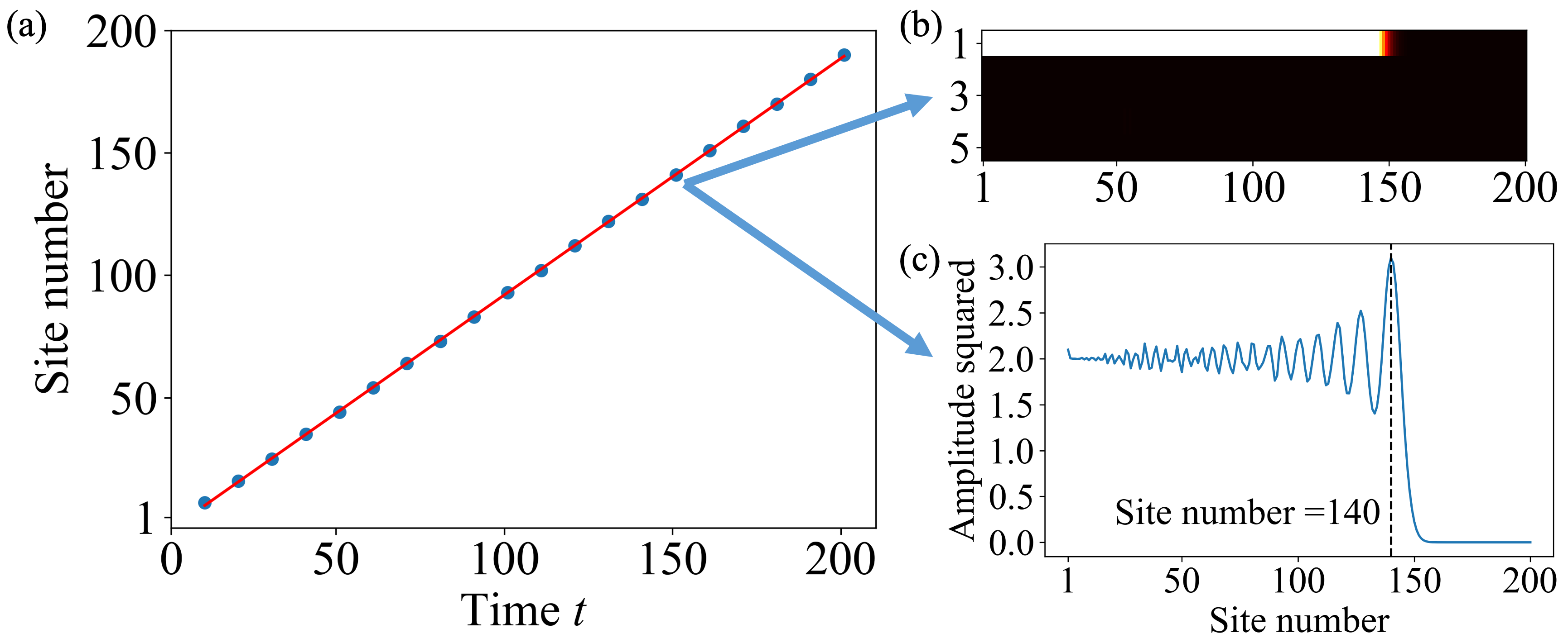
The rate of topologically guided gain is proportional to the velocity of the chirally propagating edge states, which we can measure through the advancement of the dynamical wavefront generated in the simulation. Since the velocity of the chiral modes is not affected by the non-Hermiticity or the width of the system, at least for our model, we can estimate the wavepacket velocity using the Hermitian case with , where the state suffers no attenuation and is hence more easily measured, as shown in the following Fig. S4. By plotting the amplitude squared of state at each time slice , we can obtain the movement of the wavepacket (Fig. S4(a)). Figs. S4(b) and (c) show the amplitude profile of an illustrative snapshot. The slope, 0.96, fitted shown in the red line in Fig. S4(a) indicates the velocity of the chiral propagation of the wavepacket.
S3 Generation of the disordered islands through a spatially correlated random landscape
The disordered island configurations in our work are generated by filling a random landscape up to a “sea level” of , such that regions with are dry and designed as the islands. In the following, we describe how we generate the random landscape such that the island sizes and the smoothness of their boundaries are approximately tunable via .
For any generic scalar function , one can generate [129] a real spatially-correlated random texture by multiplying the Fourier transform of with a random phase, and then taking the real part of the inverse Fourier transform of that:
| (S14) |
Here is drawn from a uniform distribution and is uncorrelated for different . Different choices of would lead to textures with different spatial correlation properties. In this work, we specialize to a Gaussian function in the - plane:
| (S15) |
From Eq. S14, one can show that the spatial correlation in obeys
| (S16) |
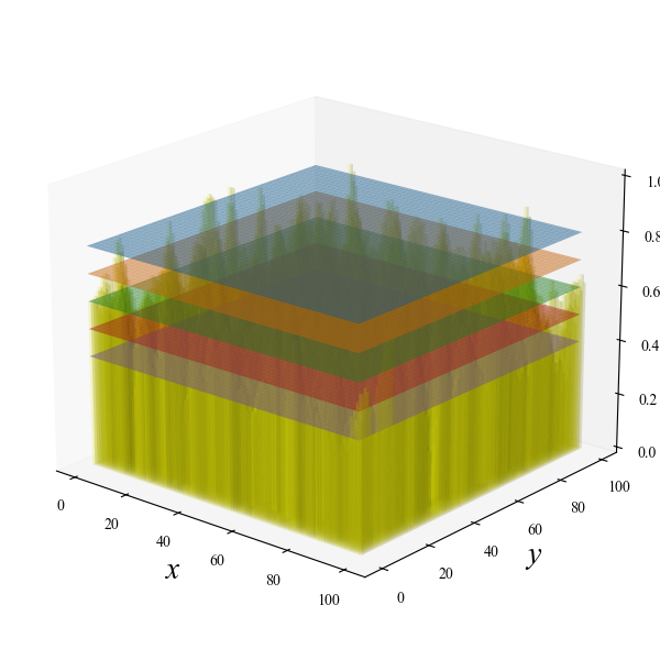
, being the correlation length, effectively controls the boundary smoothness of the islands, as shown in subfigures (a) in Figs. S5–S9 for . For simplicity, has been linearly shifted to be in the range of . It is evident that larger values of result in larger and smoother islands. Based on this random landscape, the disordered topological lattice (with both layers having identical island configurations) is generated with a “sea level” , such that the topological islands are precisely the regions where . In analogy to the sea level for an actual geographical landscape, when the sea level is very high, only the peaks above the mountains are visible, and they would form small islands. But when the sea level is lowered, the lower regions emerge from the sea and the islands grow and coalesce into larger islands, eventually forming one large island.
In Figs. S5–S9(a), the landscapes are shown inundated by the sea levels (colored in blue, orange, green, red and purple) of different values, corresponding to the island configurations shown in Figs. S5–S9(b)–(f). White regions represent topologically nontrivial islands to be implemented by with mass (such that the Chern number is [79]), while the black areas represent topologically trivial regions which are implemented as empty regions with all bonds removed. To reduce the influence of the edge effects of the system and focus solely on observing the effect caused by the topological islands, periodic boundary conditions are imposed in both the and directions. This ensures that the islands smoothly connect across the boundaries.
S3.1 Maximal island width, percolation threshold and critical sea level
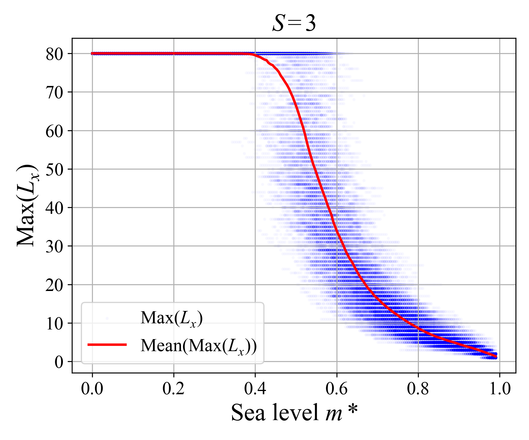
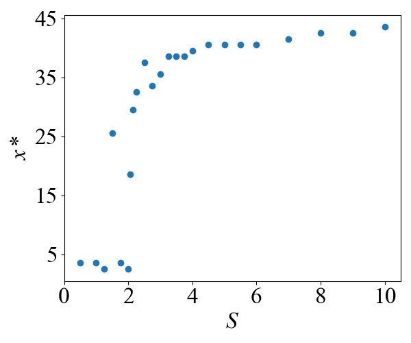
We generate a number of random lattices of size and with edge smoothness using the method described above in the Supplemental Material. We plot the possible values of Max(), which is the maximum horizontal width of the topological island, against the sea level in Fig. S10(a). The red line shows the mean value of Max() for each . We see that while gives extremely tiny islands, Max() rapidly increases as decreases, and soon saturates at the maximal system width of 80 unit cells as the islands critically coalesce.
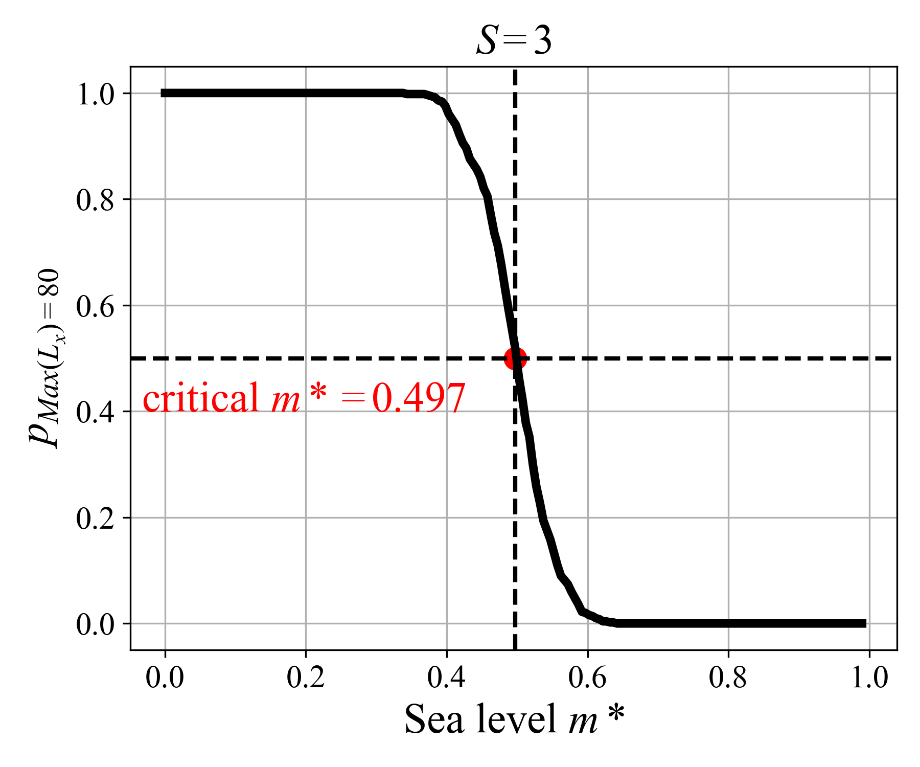
We also plot the crossing probability , which is the probability that the percolating island spans the entire lattice horizontally, against in Fig. S10(b). Note that for topologically guided gain to occur, we just need the islands to coalesce enough such that i.e. percolate across a width of , and not necessarily the whole system. We define the critical (also not to be confused with the critical width for an island to start supporting topologically guided gain) as the value where the crossing probability is , which is marked by the red circle. For , we find that the critical is , which is remarkably close to that of the square lattice percolation threshold, despite our islands being irregularly shaped.
S4 Dynamics in our disorder bilayer non-Hermitian Chern islands
Fig. S11(a) provides illustrative examples of the landscapes and islands generated by our approach above, with larger clearly leading to smoother landscapes. Figs. S11(b) depict three distinct landscapes corresponding to sea levels of , and . The spatial profiles of their midgap () eigenstates are shown in Fig. S11(b), where we clearly see that they are confined along the islands’ boundaries. Spectra colored by edge occupation ratio are shown in Fig. S11(c). The edge occupation ratio is defined in the main text Eq. (4). We observe PT symmetry breaking, characterized by the emergence of complex energies for topological edge states, in Figs. S11(c2) and (c3), where the islands have grown large enough such that their maximum width Max() is sufficiently large.
S4.1 Effect of the nonsmoothness of island boundaries on topological bulk leakage
In the main text, we have mentioned that the edge dynamics involves a competition between topologically guided propagation/gain and bulk leakage, which can lead to unlimited growth whose path is not topologically controlled. Therefore, the island boundaries cannot be excessively sharp (small ), which can overshadow the edge PT transition with bulk leakage. Here, we further show that the smoothness of the island boundaries is a key factor in determining the topological bulk leakage.
In Fig. S12(a), we show that the spatial decay length of the in-gap topological modes of our model diverge as we enter the bulk. For any eigenstate with energy , we can calculate its decay length by solving Det [48, 46, 59], where . As shown in Fig. S12, at the center of the energy gap, i.e., , is small, but as one goes closer to the bulk states near and , the decay depth gets longer as the eigenstate merges with the bulk. Hence as a system is dynamically driven, states with larger and larger decay lengths would be excited, and eventually, we excite those which are comparable to the feature size of the islands. Henceforth, we start to see significant bulk leakage.
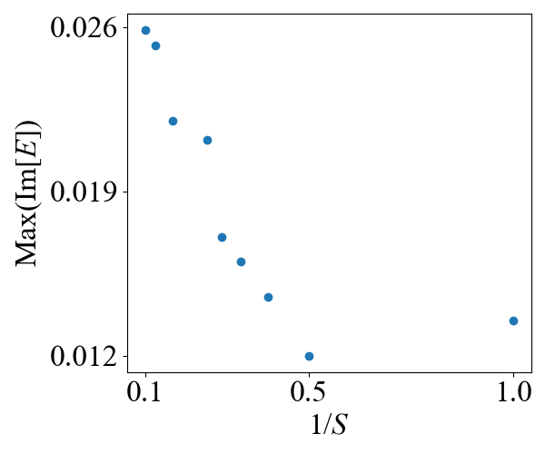
In Fig. S12(b), we see that the critical island width for gainy behavior is very small for small (sharp island features), but rapidly increases with till it saturates at large (smooth island boundaries). This is because with very small islands features characterized by small radii of curvature and inter-island distance, bulk leakage is almost imminent, and bulk eigenstates have broken PT symmetry. As island features become larger with increasing , bulk leakage becomes drastically reduced with the island features having a characteristic length scale exceeding that of of the in-gap topological modes (Fig. S12(a)). As bulk leakage is minimized, the remaining growth mechanism is topologically guided gain, and that fixes at the constant value derived in the main text. However, even though effectively saturates at large , the actual growth rate max(Im[]) from the edge states continues to increase as increases (i.e. as decreases), as shown in Fig. S12(c). This is because smoother island boundaries allow for more undisturbed topological propagation without destructive interference, and therefore topologically guided gain.
In Figs. S12(d) and (e), we show the full spectra for the and cases, which are the cases dominated by bulk leakage. For , the island features are so tiny that there is no proper distinction between the bulk and the boundaries (with most states all red). For , the bulk states (greenish blue) are clearly distinguishable from the boundary states (red), but the boundary states do not form well-defined chiral bands and the bulk states have far larger gain (Im[]). Hence the inevitably significant bulk leakage for small or .
To more concretely show how that bulk leakage is related to island width, we plot the maximum Im[] values of midgap topological edge states against the maximum island width Max() in Fig. S12(f). The maximum Im[] values of the topological edge states are indicated by empty circles, corresponding to boundary smoothness or . One does not observe a similar PT transition as those in Fig. 3(a) in the main text. The reason is that the edges are too sharp to allow for well-defined chiral Chern dynamics, such that bulk leakage dominates.
As an additional comment, bulk leakage can become much more significant if the system is too narrow, such that the islands are also inevitably narrow and interference can occur between two opposite boundaries of the island.