On invariants of constant $p$-mean curvature surfaces in the Heisenberg group $H_{1}$

Abstract.

A fundamental goal of geometry of submanifolds is to find fascinating and significant classical examples. In this paper, depending on the theory we established in [5], along with the approach we provided for constructing constant $p$-mean curvature surfaces, we found some interesting examples of constant $p$-mean curvature surfaces. In particular, we give a complete description for rotationally invariant surfaces of constant $p$-mean curvature, including the geometric meaning of the energy $E$ (1.6).

1. Introduction

This article is an extension of the previous paper [5], in which we studied the constant $p$-mean curvature surfaces in the Heisenberg groups $H_{1}$. In [5], we focused on the foundation of the theory and paid more attention to the investigation of $p$-minimal surfaces. However, in the present article, instead of theory, we mainly focus on the examples, including an approach to construct constant $p$-mean curvature surfaces.

Recall that the Heisenberg group $H_{1}$ is the space $\mathbb{R}^{3}$ associated with the group multiplication

$$(x_{1},y_{1},z_{1})\circ(x_{2},y_{2},z_{2})=(x_{1}+x_{2},y_{1}+y_{2},z_{1}+z_{2}+y_{1}x_{2}-x_{1}y_{2}),$$

which is a $3$-dimensional Lie group. The space of all left invariant vector fields is spanned by the following three vector fields:

$$\mathring{e}_{1}=\frac{\partial}{\partial x}+y\frac{\partial}{\partial z},~{}~{}\mathring{e}_{2}=\frac{\partial}{\partial y}-x\frac{\partial}{\partial z}~{}~{}\mbox{ and }~{}~{}T=\frac{\partial}{\partial z}.$$

The standard contact bundle on $H_{1}$ is the subbundle $\xi$ of the tangent bundle $TH_{1}$ spanned by $\mathring{e}_{1}$ and $\mathring{e}_{2}$. It is also defined to be the kernel of the contact form

$$\Theta=dz+xdy-ydx.$$

The CR structure on $H_{1}$ is the endomorphism $J:\xi\to\xi$ defined by

$$J(\mathring{e}_{1})=\mathring{e}_{2}~{}~{}\mbox{ and }~{}~{}J(\mathring{e}_{2})=-\mathring{e}_{1}.$$

One can view $H_{1}$ as a pseudo-hermitian manifold with $(J,\Theta)$ as the standard pseudo-hermitian structure. There is a naturally associated connection $\nabla$ if we regard all these left invariant vector fields $\mathring{e}_{1},\mathring{e}_{2}$ and $T$ as parallel vector fields. A naturally associated metric on $H_{1}$ is the adapted metric $g_{\Theta}$, which is defined by $g_{\Theta}=d\Theta(\cdot,J\cdot)+\Theta^{2}$. It is equivalent to defining the metric regarding $\mathring{e}_{1},\mathring{e}_{2}$ and $T$ as an orthonormal frame field. We sometimes use $<\cdot,\cdot>$ to denote the adapted metric. In this paper, we use the adapted metric to measure the lengths, angles of vectors, and so on.

Suppose $\Sigma$ is a surface in the Heisenberg group $H_{1}$. There is a one-form $I$ on $\Sigma$ induced from the adapted metric $g_{\Theta}$. This induced metric is defined on the whole surface $\Sigma$ and is called the first fundamental form of $\Sigma$. The intersection $T\Sigma\cap\xi$ is integrated to be a singular foliation on $\Sigma$ called the characteristic foliation. Each leaf is called a characteristic curve. A point $p\in\Sigma$ is called a singular point if at which the tangent plane $T_{p}\Sigma$ coincides with the contact plane $\xi_{p}$; otherwise, $p$ is called a regular (or non-singular) point. Generically, a point $p\in\Sigma$ is a regular point, and the set of all regular points is called the regular part of $\Sigma$. In this paper, we always assume that the surface $\Sigma$ is of $C^{2}$, but of $C^{\infty}$ on the regular part. On the regular part, we can choose a unit vector field $e_{1}$ such that $e_{1}$ defines the characteristic foliation. The vector $e_{1}$ is determined up to a sign. Let $e_{2}=Je_{1}$. Then $\{e_{1},e_{2}\}$ forms an orthonormal frame field of the contact bundle $\xi$. We usually call the vector field $e_{2}$ a horizontal normal vector field. Then the $p$-mean curvature $H$ of the surface $\Sigma$ is defined by

(1.1) $$\nabla_{e_{1}}e_{2}=-He_{1}.$$

The $p$-mean curvature $H$ is only defined on the regular part of $\Sigma$. If $H=c$, which is a constant on the whole regular part, we call the surface a constant $p$-mean curvature surface. In particular, if $c=0$, it is a $p$-minimal surface. There also exists a function $\alpha$ defined on the regular part such that $\alpha e_{2}+T$ is tangent to the surface $\Sigma$. We call this function the $\alpha$-function of $\Sigma$. It is uniquely determined up to a sign, which depends on the choice of the characteristic direction $e_{1}$. Define $\hat{e}_{1}=e_{1}$ and $\hat{e}_{2}=\frac{\alpha e_{2}+T}{\sqrt{1+\alpha^{2}}}$, then $\{\hat{e}_{1},\hat{e}_{2}\}$ forms an orthonormal frame field of the tangent bundle $T\Sigma$. Notice that $\hat{e}_{2}$ is uniquely determined and independent of the choice of the characteristic direction $e_{1}$. In [2, 4], it was shown that these three invariants,

$$I,e_{1},\alpha,$$

form a complete set of invariants for constant $p$-mean curvature surfaces with $H=c$ in $H_{1}$. In particular, if $\Sigma\subset H_{1}$ is a constant $p$-mean curvature surface with $H=c$, then in terms of a compatible coordinate system $(U;x,y)$, which means

$$e_{1}=\frac{\partial}{\partial x},$$

the integrability condition (see [5]) is reduced to

(1.2) $$\begin{split}-a_{x}+a\frac{b_{x}}{b}&=\frac{c\alpha}{(1+\alpha^{2})^{1/2}},\\ -\frac{b_{x}}{b}&=2\alpha+\frac{\alpha\alpha_{x}}{1+\alpha^{2}},\\ \alpha_{xx}+6\alpha\alpha_{x}&+4\alpha^{3}+c^{2}\alpha=0,\end{split}$$

where the two functions $a$ and $b$ are a representation of the first fundamental form $I$ in the following sense that they describe the vector field

(1.3) $$\hat{e}_{2}=a(x,y)\frac{\partial}{\partial x}+b(x,y)\frac{\partial}{\partial y}.$$

In other words, there exists the $\alpha$ satisfying the Codazzi-like equation

(1.4) $$\alpha_{xx}+6\alpha\alpha_{x}+4\alpha^{3}+c^{2}\alpha=0,$$

which is a nonlinear ordinary differential equation. In [5], we normalized $a$ and $b$ such that they can be uniquely determined by the function $\alpha$, and hence we obtained the result that the existence of a constant $p$-mean curvature surface (without singular points) is equivalent to the existence of a solution to a nonlinear second-order ODE (1.4), which is a kind of Liénard equations (cf. [6]). They are one-to-one correspondences in some sense. For a detailed description, see Theorem 1.1, Theorem 1.3, and Theorem 6.3 in [5]. This result tells us that the investigation of the geometry of constant $p$-mean curvature surfaces in $H_{1}$ is equal to the study of the solution of the equation (1.4). More specifically, we obtained a complete set of solutions (see Theorem 1.2 and Theorem 1.4 in [5], or Theorem 2.1) and used the types of the solutions to the equation to divide the constant $p$-mean curvature surfaces into several classes, which are vertical, special type I, special type II and general type (see Definition 5.1 and 5.2 in [5] for $p$-minimal cases and see Definition 2.2 and 2.3 for the cases which $c\neq 0$). After the process of normalization, we obtained a complete set of invariants from the normal form of the $\alpha$-function. It is worth of our mention that the invariants in some sense measure how different a constant $p$-mean curvature surface is from the model case, which is the horizontal plane in $p$-minimal case, and the Pansu sphere in the case $c>0$.

We first study the rotationally invariant surface in $H_{1}$ with constant $p$-mean curvature $H=c$ using the Codazzi-like equation (1.4). In [7], M. Ritoré and C. Rosales made an investigation on such kinds of surfaces by a first-order ODE system. In the present paper, we shall study them again from the point of view of our theory established in the previous paper [5] and the present one. Let $\Sigma(s,\theta)$ be a rotationally invariant surface in $H_{1}$ with $H=c$, generated by a generating curve $\gamma(s)=(x(s),0,t(s)),\ x(s)\geq 0$, on the $xt$-plane, that is, $\Sigma$ is parametrized by

(1.5) $$\Sigma(s,\theta)=(x(s)\cos\theta,x(s)\sin\theta,t(s)),$$

where $x^{\prime 2}+t^{\prime 2}=1$. Here ^′ means taking a derivative with respect to $s$. Recall the energy

(1.6) $$E=\frac{xt^{\prime}}{\sqrt{x^{2}x^{\prime 2}+t^{\prime 2}}}+\lambda x^{2},$$

which was introduced in [7] and was shown to be a constant. Here $2\lambda=c$ and notice that our $p$-mean curvature differs from the one defined in [7] by a sign. We hence have Theorem A and Theorem B that follow from section 3.

Theorem A: A curve $\gamma=(x,t)$ is the generating curve of a rotationally invariant surface $\Sigma$ in $H_{1}$ with $H=c\neq 0$ if and only if $\gamma=(x,t)$ is defined by

(1.7) $$\begin{split}x^{2}&=\frac{k}{c^{2}}+r\cos{(c\tilde{s})},\\ t&=-\frac{\tilde{s}}{c}-\frac{r}{2}\sin{(c\tilde{s})},\ \textrm{up to a constant}.\end{split}$$

for some horizontal arc-length parameter $\tilde{s}$ and some $k,r\in\operatorname{\mathbb{R}},\ r>0$. In addition, we have

(1.8) $$k=2cE+2.$$

If $r=0$, then $\Sigma$ is a cylinder. If $r\neq 0$, then, in terms of a normal coordinates $(\bar{s},\bar{\theta})$, the two invariants for $\Sigma$ are

(1.9) $$\begin{split}\zeta_{1}(\bar{\theta})&=-\frac{2E\bar{\theta}}{cr},\ \textrm{up to a constant, which is linear on $\bar{\theta}$},\\ \zeta_{2}(\bar{\theta})&=-\frac{2cE+2}{c^{2}r},\ \textrm{which is a constant}.\end{split}$$

Theorem B: A curve $\gamma=(x,t)$ is the generating curve of a rotationally invariant $p$-minimal surface $\Sigma$ in $H_{1}$ if and only if either $t$ is a constant, and hence $\Sigma$ is a part of the horizontal plane, or $\gamma=(x,t)$ is defined by

(1.10) $$\begin{split}x^{2}&=\tilde{s}^{2}+c_{2},\\ t&=m\tilde{s},\ \textrm{up to a constant},\end{split}$$

for some horizontal arc-length parameter $\tilde{s}$ and some $c_{2},m\in\operatorname{\mathbb{R}},\ m\neq 0$. In addition, we have

(1.11) $$E=m.$$

In terms of a normal coordinates $(\bar{s},\bar{\theta})$, the two invariants for $\Sigma$ are

(1.12) $$\begin{split}\zeta_{1}(\bar{\theta})&=E\bar{\theta},\ \textrm{up to a constant, which is linear on $\bar{\theta}$},\\ \zeta_{2}(\bar{\theta})&=c_{2},\ \textrm{which is a constant}.\end{split}$$

For more interesting examples, in section 4, we provide an approach to construct a constant $p$-mean curvature surface. This approach is an analog of the one we performed in the previous paper [5] for $p$-minimal surfaces. Actually in [5] we deformed the horizontal plane along a curve $\mathcal{C}(\theta)=(x_{1}(\theta),x_{2}(\theta),x_{3}(\theta))$ to obtain a $p$-minimal surface. Recall that in Section 9 in [5], depending on a parametrized curve $\mathcal{C}(\theta)=(x_{1}(\theta),x_{2}(\theta),x_{3}(\theta))$ for $\theta\in\operatorname{\mathbb{R}}$, we deformed the graph $u=0$ to obtain a $p$-minimal surface parametrized by

(1.13) $$Y(r,\theta)=(x_{1}(\theta)+r\cos{\theta},x_{2}(\theta)+r\sin{\theta},x_{3}(\theta)+rx_{2}(\theta)\cos{\theta}-rx_{1}(\theta)\sin{\theta}),$$

for $r\in\operatorname{\mathbb{R}}$. It is easy to checked that $Y$ is an immersion if and only if either $\Theta(\mathcal{C}^{\prime}(\theta))-(x_{2}^{\prime}(\theta)\cos{\theta}-x_{1}^{\prime}(\theta)\sin{\theta})^{2}\neq 0\ \textrm{or}\ r+(x_{2}^{\prime}(\theta)\cos{\theta}-x_{1}^{\prime}(\theta)\sin{\theta})\neq 0$ for all $\theta$. In particular, the surface $Y$ defines a $p$-minimal surface of special type I if the curve $\mathcal{C}$ satisfies

(1.14) $$x_{3}^{\prime}(\theta)+x_{1}(\theta)x_{2}^{\prime}(\theta)-x_{2}(\theta)x_{1}^{\prime}(\theta)-(x_{2}^{\prime}(\theta)\cos{\theta}-x_{1}^{\prime}(\theta)\sin{\theta})^{2}=0,$$

for all $\theta$. In addition, the corresponding $\zeta_{1}$-invariant reads

(1.15) $$\zeta_{1}(\theta)=x_{2}^{\prime}(\theta)\cos{\theta}-x_{1}^{\prime}(\theta)\sin{\theta}-\int\big{[}x_{1}^{\prime}(\theta)\cos{\theta}+x_{2}^{\prime}(\theta)\sin{\theta}\big{]}d\theta.$$

Similarly, the surface $Y$ defines a $p$-minimal surface of general type if the curve $\mathcal{C}$ satisfies

(1.16) $$x_{3}^{\prime}(\theta)+x_{1}(\theta)x_{2}^{\prime}(\theta)-x_{2}(\theta)x_{1}^{\prime}(\theta)-(x_{2}^{\prime}(\theta)\cos{\theta}-x_{1}^{\prime}(\theta)\sin{\theta})^{2}\neq 0,$$

for all $\theta$. In addition, the corresponding $\zeta_{1}$- and $\zeta_{2}$-invariant read

(1.17) $$\left\{\begin{split}\zeta_{1}(\theta)&=x_{2}^{\prime}(\theta)\cos{\theta}-x_{1}^{\prime}(\theta)\sin{\theta}-\int\big{[}x_{1}^{\prime}(\theta)\cos{\theta}+x_{2}^{\prime}(\theta)\sin{\theta}\big{]}d\theta\\ \zeta_{2}(\theta)&=x_{3}^{\prime}(\theta)+x_{1}(\theta)x_{2}^{\prime}(\theta)-x_{2}(\theta)x_{1}^{\prime}(\theta)-(x_{2}^{\prime}(\theta)\cos{\theta}-x_{1}^{\prime}(\theta)\sin{\theta})^{2}.\end{split}\right.$$

In section 4, we are going to construct a constant $p$-mean curvature surface by perturbing the Pansu sphere along a given curve $\mathcal{C}(\theta)$. In subsection 2.2, we see that the Pansu sphere can be parametrized by

(1.18) $$X(s,\theta)=\left(\begin{array}[]{ccc}\cos\theta&-\sin\theta&0\\ \sin\theta&\cos\theta&0\\ 0&0&1\end{array}\right)\left(\begin{array}[]{c}x(s)\\ y(s)\\ t(s)\end{array}\right)=\left(\begin{array}[]{c}x(s)\cos\theta-y(s)\sin\theta\\ x(s)\sin\theta+y(s)\cos\theta\\ t(s)\end{array}\right),$$

where

(1.19) $$\left\{\begin{array}[]{ccl}x(s)&=&\frac{1}{2\lambda}\sin(2\lambda s)\\ y(s)&=&-\frac{1}{2\lambda}\cos(2\lambda s)+\frac{1}{2\lambda}\\ t(s)&=&\frac{1}{4\lambda^{2}}\sin(2\lambda s)-\frac{1}{2\lambda}s+\frac{\pi}{4\lambda^{2}},\end{array}\right.$$

with $X(0,\theta)=(0,0,\frac{\pi}{4\lambda^{2}})$ and $X(\frac{\pi}{\lambda},\theta)=(0,0,-\frac{\pi}{4\lambda^{2}})$ as the North pole and South pole, respectively. In section 4 we deform it along $\mathcal{C}(\theta)=(x_{1}(\theta),x_{2}(\theta),x_{3}(\theta))$ to obtain a constant $p$-mean curvature surface $Y(s,\theta)$ as follows.

(1.20) $$\begin{split}Y(s,\theta)&=\Big{(}x_{1}(\theta)+\big{(}x(s)\cos{\theta}-y(s)\sin{\theta}\big{)},x_{2}(\theta)+\big{(}x(s)\sin{\theta}+y(s)\cos{\theta}\big{)},\\ &x_{3}(\theta)+t(s)+x_{2}(\theta)\big{(}x(s)\cos{\theta}-y(s)\sin{\theta}\big{)}-x_{1}(\theta)\big{(}x(s)\sin{\theta}+y(s)\cos{\theta}\big{)}\Big{)}.\end{split}$$

We also give a condition for $Y$ to be an immersion. The coordinates $(s,\theta)$ for $Y$ is a compatible coordinate system. We have (see (4.6))

(1.21) $$\alpha=\lambda\frac{A(\theta)\cos{2\lambda s}+\left(\frac{1}{2\lambda}-B(\theta)\right)\sin{2\lambda s}}{\left(B(\theta)-\frac{1}{2\lambda}\right)\cos{2\lambda s}+A(\theta)\sin{2\lambda s}+D(\theta)},$$

where

(1.22) $$\begin{split}A(\theta)&=x^{\prime}_{2}(\theta)\cos{\theta}-x^{\prime}_{1}(\theta)\sin{\theta},\ \ B(\theta)=x^{\prime}_{2}(\theta)\sin{\theta}+x^{\prime}_{1}(\theta)\cos{\theta},\\ D(\theta)&=\lambda\Theta(\mathcal{C}^{\prime}(\theta))+\left(\frac{1}{2\lambda}-B(\theta)\right),\ \ V(\theta)=\left(A(\theta),\frac{1}{2\lambda}-B(\theta)\right).\end{split}$$

If $V(\theta)=0$, then $\alpha=0$, and hence $Y$ is a cylinder. If $V(\theta)\neq 0$, then we define

$$\left\|V(\theta)\right\|=\sqrt{\left[A\left(\theta\right)\right]^{2}+\left[\frac{1}{2\lambda}-B(\theta)\right]^{2}}$$

and write

$$G(\theta)=\frac{D(\theta)}{\left\|V(\theta)\right\|},\ \ \frac{V(\theta)}{\left\|V(\theta)\right\|}=\big{(}\sin{\zeta(\theta)},\cos{\zeta(\theta)}\big{)},$$

for some function $\zeta{(\theta)}$. From (1.21), we thus have

$$\alpha=\lambda\frac{\sin{\big{(}2\lambda s+\zeta{(\theta)}\big{)}}}{G(\theta)-\cos{\big{(}2\lambda s+\zeta{(\theta)}\big{)}}}.$$

Finally, we normalize the $\alpha$-function to obtain the two invariants for $Y$, stated in Theorem 4.1. We list it here as the third main result of the present paper.

Theorem C: If $V=0$, then $\alpha=0$. If $V\neq 0$, then we consider the new coordinates

$$\tilde{s}=s+\Gamma(\theta),\ \ \tilde{\theta}=\Psi(\theta),$$

where

$$\Gamma(\theta)=\frac{\theta}{2\lambda}-\int D(\theta)d\theta,\ \ \Psi(\theta)=2\lambda\int\left\|V(\theta)\right\|d\theta,$$

then the coordinates $(\tilde{s},\tilde{\theta})$ is normal. In terms of the normal coordinates, the invariants of $Y$ are given by

(1.23) $$\left\{\begin{array}[]{lll}\zeta_{1}\left(\tilde{\theta}\right)&=&\zeta\left(\theta\right)-2\lambda\Gamma\left(\theta\right),\\ \zeta_{2}\left(\tilde{\theta}\right)&=&G\left(\theta\right),\end{array}\right.$$

where $\theta=\Psi^{-1}\left(\tilde{\theta}\right)$.

In section 5, we use formula (1.15), (1.17) and (1.23) to construct various examples of surfaces of constant $p$-mean curvature including degenerate p-minimal surfaces of special type I.

Acknowledgments. The first author’s research was supported in part by NSTC 112-2115-M-007-009-MY3. The second author’s research was supported in part by NSTC 110-2115-M-167-002-MY2 and NSTC 112-2115-M-167-002-MY2. The third author’s research was supported in part by NSTC 112-2628-M-032-001-MY4.

2. Solutions to the Codazzi-like equation

The Codazzi-like equation for a surface in $H_{1}$ with constant $p$-mean curvature $H=c>0$ is

(2.1) $$\alpha_{xx}+6\alpha\alpha_{x}+4\alpha^{3}+c^{2}\alpha=0.$$

Theorem 2.1.

[5] Besides the following three special solutions to (2.1),

$$\alpha(x)=0,\ -\frac{c}{2}\tan(cx+cK_{1}),\ \alpha(x)=-\frac{c}{2}\tan(\frac{c}{2}x-\frac{c}{2}K_{2}),$$

we have the general solution to (2.1) of the form

(2.2) $$\alpha(x)=\frac{c}{2}\frac{\sin{\big{(}cx+c_{1}\big{)}}}{c_{2}-\cos{\big{(}cx+c_{1}\big{)}}},$$

which depends on constants $K_{1}$,$K_{2},c_{1}$, and $c_{2}$.

Note that all the solutions are a periodic function with $\alpha(x+\frac{2\pi}{c})=\alpha(x)$ for all $x$. We give some remarks as follows.

1. In terms of the following identities

   $$\begin{split}-\tan{(\theta+\frac{\pi}{2})}&=\cot{\theta}=\frac{\sin{2\theta}}{1-\cos{2\theta}},\\ -\tan{2\theta}&=-\frac{\sin{2\theta}}{\cos{2\theta}}=\frac{\sin{2\theta}}{0-\cos{2\theta}},\end{split}$$

   we see that the two nontrivial special solutions in Theorem 2.1 correspond to the general solution in Theorem 2.1 with $c_{2}=0$ and $c_{2}=1$, respectively.

2. From the following identity

   $$\frac{\sin{(\theta+\pi)}}{c_{2}-\cos{(\theta+\pi)}}=\frac{\sin{\theta}}{-c_{2}-\cos{\theta}},$$

   we can assume without loss of generality that $c_{2}\geq 0$ in the general solution.

Due to Theorem 2.1, we are able to use the types of the solutions to (2.1) to classify the constant $p$-mean curvature surfaces into several classes, which are vertical, special type I, special type II and general type. In terms of compatible coordinates $(x,y)$, the function $\alpha(x,y)$ is a solution to the Codazzi-like equation (2.1) for any given $y$. By Theorem 2.1, the function $\alpha(x,y)$ hence has one of the following forms of special types

$$0,\ \frac{c}{2}\frac{\sin(cx+c_{1})}{0-\cos(cx+c_{1})},\ \frac{c}{2}\frac{\sin{(cx+c_{1})}}{1-\cos{\big{(}cx+c_{1})}},$$

and general types

$$\frac{c}{2}\frac{\sin{(cx+c_{1})}}{c_{2}-\cos{(c(x+c_{1})}},$$

where, instead of constants, both $c_{1}$ and $c_{2}$ are now functions of $y$. Notice that it is convenient at some point to assume that $c_{2}(y)\geq 0$ for all $y$. We now use the types of the function $\alpha(x,y)$ to define the types of constant $p$-mean curvature surfaces as follows.

Definition 2.2.

Locally, we say that a constant $p$-mean curvature surface is

1. vertical if $\alpha$ vanishes (i.e., $\alpha(x,y)=0$ for all $x,y$);
   

2. of special type I if $\alpha=\frac{c}{2}\frac{\sin{(cx+c_{1})}}{1-\cos{(cx+c_{1})}}$;
   

3. of special type II if $\alpha=\frac{c}{2}\frac{\sin(cx+c_{1})}{0-\cos(cx+c_{1})}$;
   

4. of general type if $\alpha=\frac{c}{2}\frac{\sin{(cx+c_{1})}}{c_{2}-\cos{(cx+c_{1})}}$ with $c_{2}(y)\notin\{0,1\}$ for all $y$.

We further divide constant $p$-mean curvature surfaces of general type into three classes as follows:

Definition 2.3.

A constant $p$-mean curvature surface of general type is

1. of type I if $c_{2}(y)>1$ for all $y$;
   

2. of type II if $0<c_{2}(y)<1$ for all $y$, and $\frac{-c_{1}+\cos^{-1}c_{2}}{c}<x<\frac{2\pi-c_{1}-\cos^{-1}c_{2}}{c}$;
   

3. of type III if $0<c_{2}(y)<1$ for all $y$, and either $\frac{-c_{1}}{c}\leq x<\frac{-c_{1}+\cos^{-1}c_{2}}{c}$ or
   $\frac{2\pi-c_{1}-\cos^{-1}c_{2}}{c}<x\leq\frac{-c_{1}+2\pi}{c}$.

where $\cos^{-1}$ is the inverse of the function $\cos:[0,\pi]\rightarrow[-1,1]$.

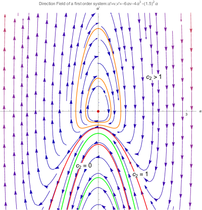
Figure 1. Direction field for c=1.5

We notice that the type is invariant under the action of a Heisenberg rigid motion and the regular part of a constant $p$-mean curvature surface $\Sigma\subset H_{1}$ is a union of these types of surfaces. The corresponding paths of each type of $\alpha$ are shown on the phase plane (Figure 1). We express some basic facts as follows.

• If $\alpha$ vanishes, then it is part of a vertical cylinder.

• The two concave downward parabolas in red represent

  $$\alpha=\frac{c}{2}\frac{\sin{(cx+c_{1})}}{1-\cos{(cx+c_{1})}},\frac{c}{2}\frac{\sin{(cx+c_{1})}}{0-\cos{(cx+c_{1})}},$$

  respectively. The one for $\alpha=\frac{c}{2}\frac{\sin{(cx+c_{1})}}{1-\cos{(cx+c_{1})}}$ is above the one for $\alpha=\frac{c}{2}\frac{\sin{(cx+c_{1})}}{0-\cos{(cx+c_{1})}}$. For surfaces of special type I, we have that

  $$\alpha(\frac{\pi-c_{1}}{c})=0,\ \alpha^{\prime}(\frac{\pi-c_{1}}{c})=-\frac{c^{2}}{4}$$

  and

  (2.3) $$\begin{split}\alpha\rightarrow\left\{\begin{array}[]{rl}\infty,&\ \text{if}\ x\rightarrow\frac{-c_{1}}{c}\ \ \text{from the right},\\ &\\ -\infty,&\ \text{if}\ x\rightarrow\frac{2\pi-c_{1}}{c}\ \ \text{from the left},\end{array}\right.\end{split}$$

  and, for surfaces of special type II in which $\alpha$ has period $\pi$, we have that

  $$\alpha(\frac{-c_{1}}{c})=\alpha(\frac{\pi-c_{1}}{c})=0,\ \alpha^{\prime}(\frac{-c_{1}}{c})=\alpha^{\prime}(\frac{\pi-c_{1}}{c})=-\frac{c^{2}}{2}$$

  and

  (2.4) $$\begin{split}\alpha\rightarrow\left\{\begin{array}[]{rl}\infty,&\ \text{if}\ x\rightarrow\frac{\pi-2c_{1}}{2c}\ \ \text{from the right},\\ &\\ -\infty,&\ \text{if}\ x\rightarrow\frac{3\pi-2c_{1}}{2c}\ \ \text{from the left},\end{array}\right.\end{split}$$

• The closed curves in orange on the phase plane correspond to the family of solutions

  $$\alpha(x)=\frac{c}{2}\frac{\sin{(cx+c_{1})}}{c_{2}-\cos{(cx+c_{1})}},$$

  where $c_{1},c_{2}$ are constants and $c_{2}>1$, which are of type I. There exist zeros for $\alpha$-function at $x=\frac{-c_{1}}{c},\ \frac{\pi-c_{1}}{c}$, at which we have that

  $$\alpha^{\prime}(\frac{-c_{1}}{c})=\frac{1}{2}\frac{c^{2}}{c_{2}-1}>0,\ \ \ \alpha^{\prime}(\frac{\pi-c_{1}}{c})=-\frac{1}{2}\frac{c^{2}}{c_{2}+1}<0,$$

  There are no singular points for surfaces of type I.

• The curves in between the two red concave downward parabolas are of type II. The $\alpha$-function of type II has a zero at $x=\frac{\pi-c_{1}}{c}$, and

  $$\alpha^{\prime}(\frac{\pi-c_{1}}{c})=-\frac{1}{2}\frac{c^{2}}{c_{2}+1}<0.$$

  For surfaces of type II, it can be checked that

  (2.5) $$\begin{split}\alpha\rightarrow\left\{\begin{array}[]{rl}\infty,&\ \text{if}\ x\rightarrow\frac{-c_{1}+\cos^{-1}c_{2}}{c}\ \ \text{from the right},\\ &\\ -\infty,&\ \text{if}\ x\rightarrow\frac{-c_{1}+2\pi-\cos^{-1}c_{2}}{c}\ \ \text{from the left}.\end{array}\right.\end{split}$$

• The curves beneath the lower concave downward parabola are of type III. There exists a zero for $\alpha$-function at $x=\frac{-c_{1}}{c}$, and

  $$\alpha^{\prime}(\frac{-c_{1}}{c})=\frac{1}{2}\frac{c^{2}}{c_{2}-1}<0.$$

  For surfaces of type III, we have

  (2.6) $$\begin{split}\alpha\rightarrow\left\{\begin{array}[]{rl}-\infty,&\ \text{if}\ x\rightarrow\frac{-c_{1}+\cos^{-1}c_{2}}{c}\ \ \text{from the left},\\ &\\ \infty,&\ \text{if}\ x\rightarrow\frac{-c_{1}+2\pi-\cos^{-1}c_{2}}{c}\ \ \text{from the right}.\end{array}\right.\end{split}$$

2.1. The structure of the singular sets

In this subsection, we study the structure of the singular set. For the general type, we choose a normal coordinate system $(s,\theta)$ such that

(2.7) $$\alpha=\lambda\frac{\sin\left(2\lambda s+\zeta_{1}(\theta)\right)}{\zeta_{2}(\theta)-\cos\left(2\lambda s+\zeta_{1}(\theta)\right)},$$

and

$$a=-\frac{\lambda}{\sqrt{1+\alpha^{2}}},\text{ }b=\frac{2\lambda^{2}}{\left|\zeta_{2}\left(\theta\right)-\cos\left(2\lambda s+\zeta_{1}\left(\theta\right)\right)\right|\sqrt{1+\alpha^{2}}}.$$

Then the singular set is the graph of the function

$$x\left(\theta\right)=\frac{\cos^{-1}\left(\zeta_{2}(\theta)\right)-\zeta_{1}(\theta)}{2\lambda}.$$

The induced metric $I$ (or the first fundamental form) on the regular part reads

$$I=ds\otimes ds-\frac{a}{b}ds\otimes d\theta-\frac{a}{b}d\theta\otimes ds+\frac{\left(1+a^{2}\right)}{b^{2}}d\theta\otimes d\theta.$$

Now we use the metric to compute the length of the singular set $\left\{\left(\frac{\cos^{-1}\left(\zeta_{2}(\theta)\right)-\zeta_{1}(\theta)}{2\lambda},\theta\right)\right\}$, where $\theta$ belongs to some open interval.

Case $\zeta_{2}\left(\theta\right)\neq 1$:

Let $\gamma(\theta)=\left(\frac{\cos^{-1}\left(\zeta_{2}(\theta)\right)-\zeta_{1}(\theta)}{2\lambda},\theta\right)$, which is a parametrization of the singular set. Then the square of the velocity at $\theta$ is

$$\left|\gamma^{\prime}(\theta)\right|^{2} = \left[q^{\prime}\left(\theta\right)\right]^{2}-\frac{2aq^{\prime}\left(\theta\right)}{b}+\frac{a^{2}+1}{b^{2}}$$

$$= \frac{\left[a-bq^{\prime}\left(\theta\right)\right]^{2}+1}{b^{2}}>0\text{ for all }\theta,\text{ }$$

where

$$q^{\prime}\left(\theta\right)=\left[\frac{\cos^{-1}\left(\zeta_{2}(\theta)\right)-\zeta_{1}(\theta)}{2\lambda}\right]^{\prime}=\frac{-\zeta_{2}^{{}^{\prime}}\left(\theta\right)}{2\lambda\sqrt{1-\zeta_{2}^{2}\left(\theta\right)}}-\frac{\zeta_{1}^{{}^{\prime}}\left(\theta\right)}{2\lambda}.$$

Formula (Case $\zeta_{2}\left(\theta\right)\neq 1$: ) shows that the parametrized curve $\gamma(\theta)$ of the singular set has a positive length.

Case $\zeta_{2}\left(\theta\right)=1$:

We parametrize the singular set by $\gamma(\theta)=\left(\frac{\cos^{-1}\left(1-\epsilon\right)-\zeta_{1}(\theta)}{2\lambda},\theta\right)$ for $\epsilon>0$. It is easy to see

$$\gamma^{\prime}\left(\theta\right)=\left(\frac{-\zeta_{1}^{\prime}\left(\theta\right)}{2\lambda},1\right).$$

When $\varepsilon\rightarrow 0$, the metric

$$I=ds\otimes ds-\frac{a}{b}ds\otimes d\theta-\frac{a}{b}d\theta\otimes ds+\frac{\left(1+a^{2}\right)}{b^{2}}d\theta\otimes d\theta$$

degenerates to

$$\tilde{I}=ds\otimes ds.$$

Then the square of the velocity at $\theta$ is

$$|\gamma^{\prime}\left(\theta\right)|^{2}=\frac{\left[\zeta_{1}^{\prime}\left(\theta\right)\right]^{2}}{4\lambda^{2}}.$$

Thus, if $\zeta_{1}\left(\theta\right)=c_{1}$ and $\zeta_{2}\left(\theta\right)=1$, the length of the parametrized curve $\gamma(\theta)$ of the singular set is zero. This result coincides with the singular set of the Pansu Sphere being isolated. We conclude the above discussion by the following theorem, an analog of Theorem 1.7 in [5].

Theorem 2.4.

The singular set of a constant $p$-mean surface with $H=c\neq 0$ is either

1. an isolated point; or

2. a smooth curve.

In addition, an isolated singular point only happens on the surfaces of special type I with $\zeta_{1}=\textrm{const.}$, namely, a part of the Pansu sphere contains the poles as the isolated singular point.

Theorem 2.4 together with Theorem 1.7 in [5] is just a special case of Theorem 3.3 in [3]. However, we give a computable proof of this result for constant $p$-mean surfaces. We also have the description of how a characteristic leaf goes through a singular curve, which is called a ”go through” theorem in [3]. Suppose $p_{0}$ is a point belonging to a singular curve. From the above basic facts, we see that a characteristic curve $\gamma$ always reaches the singular point $p_{0}$ going a finite distance. From the opposite direction, suppose $\tilde{\gamma}$ is another characteristic curve that reaches $p_{0}$. Then the union of $\gamma,p_{0}$ and $\tilde{\gamma}$ forms a smooth curve (we also refer the reader to the proof of Theorem 1.8 in [5], they are similar). We thus have the following theorem.

Theorem 2.5.

Let $\Sigma\subset H_{1}$ be a constant $p$-mean surface with $H=c\neq 0$. Then the characteristic foliation is smooth around the singular curve in the following sense that each leaf can be extended smoothly to a point on the singular curve.

Making use of Theorem 2.5, we have the following result.

Theorem 2.6.

Let $\Sigma$ be a constant $p$-mean surface of type II $($III$)$ with $H=c\neq 0$. If it can be smoothly extended through the singular curve, then the other side of the singular curve is of type III $($II$)$.

Therefore, we see that a surface of general type $II$ is always pasted together with a surface of general type $III$ at a singular curve and vice versa.

2.2. The Pansu Sphere

Lemma 2.7 (Pansu Sphere).

A Pansu sphere has its $\alpha$-function of special type I. In fact, we have

(2.9) $$\alpha=\frac{\lambda\sin(2\lambda s)}{(1-\cos(2\lambda s))},\ a=\frac{-\lambda}{\sqrt{1+\alpha^{2}}},\ b=\frac{2\lambda^{2}}{\sqrt{1+\alpha^{2}}(1-\cos{2\lambda s})}$$

Proof.

A Pansu sphere is given in [1] by

$$f(z)=\frac{1}{2\lambda^{2}}\left(\lambda|z|\sqrt{1-\lambda^{2}|z|^{2}}+\cos^{-1}(\lambda|z|)\right),|z|\leq\frac{1}{\lambda},$$

which has a constant $p$-mean curvature $c=2\lambda$. It can be parametrized by

(2.10) $$X(s,\theta)=\left(\begin{array}[]{ccc}\cos\theta&-\sin\theta&0\\ \sin\theta&\cos\theta&0\\ 0&0&1\end{array}\right)\left(\begin{array}[]{c}x(s)\\ y(s)\\ t(s)\end{array}\right)=\left(\begin{array}[]{c}x(s)\cos\theta-y(s)\sin\theta\\ x(s)\sin\theta+y(s)\cos\theta\\ t(s)\end{array}\right),$$

where

(2.11) $$\left\{\begin{array}[]{ccl}x(s)&=&\frac{1}{2\lambda}\sin(2\lambda s)\\ y(s)&=&-\frac{1}{2\lambda}\cos(2\lambda s)+\frac{1}{2\lambda}\\ t(s)&=&\frac{1}{4\lambda^{2}}\sin(2\lambda s)-\frac{1}{2\lambda}s+\frac{\pi}{4\lambda^{2}}\end{array}\right.,$$

with $X(0,\theta)=(0,0,\frac{\pi}{4\lambda^{2}})$ and $X(\frac{\pi}{\lambda},\theta)=(0,0,-\frac{\pi}{4\lambda^{2}})$ as the North pole and South pole, respectively. We then have $e_{1}:=X_{s}$, which means that $X(s,\theta)$ defines a compatible coordinate system. Moreover, $e_{2}=Je_{1}$, where

(2.12) $$\begin{split}e_{1}&=X_{s}=(x^{\prime}(s)\cos\theta-y^{\prime}(s)\sin\theta,x^{\prime}(s)\sin\theta+y^{\prime}(s)\cos\theta,t^{\prime}(s))\\ &=(x^{\prime}(s)\cos\theta-y^{\prime}(s)\sin\theta)\mathring{e}_{1}+(x^{\prime}(s)\sin\theta+y^{\prime}(s)\cos\theta)\mathring{e}_{2}|_{X(s,\theta)},\\ e_{2}&=-(x^{\prime}(s)\sin\theta+y^{\prime}(s)\cos\theta)\mathring{e}_{1}+(x^{\prime}(s)\cos\theta-y^{\prime}(s)\sin\theta)\mathring{e}_{2}.\end{split}$$

We note that $\alpha$ is a function satisfying

(2.13) $$\alpha e_{2}+T=\mathcal{A}X_{s}+\mathcal{B}X_{\theta},$$

for some functions $\mathcal{A}$ and $\mathcal{B}$. Direct calculation shows that

(2.14) $$X_{\theta}=(-x(s)\sin\theta-y(s)\cos\theta)\mathring{e}_{1}+(x(s)\cos\theta-y(s)\sin\theta)\mathring{e}_{2}+(x^{2}(s)+y^{2}(s))T.$$

Therefore, (2.13) implies

(2.15) $$\begin{split}-\alpha(x^{\prime}(s)\sin\theta+y^{\prime}(s)\cos\theta)&=\mathcal{A}(x^{\prime}(s)\cos\theta-y^{\prime}(s)\sin\theta)+\mathcal{B}(-x(s)\sin\theta-y(s)\cos\theta)\\ \alpha(x^{\prime}(s)\cos\theta-y^{\prime}(s)\sin\theta)&=\mathcal{A}(x^{\prime}(s)\sin\theta+y^{\prime}(s)\cos\theta)+\mathcal{B}(x(s)\cos\theta-y(s)\sin\theta)\\ 1&=\mathcal{B}(x^{2}(s)+y^{2}(s)).\end{split}$$

The last equation of (2.15) yields

$$\mathcal{B}=\frac{1}{x^{2}(s)+y^{2}(s)},$$

and hence

$$b=\frac{\mathcal{B}}{\sqrt{1+\alpha^{2}}}=\frac{2\lambda^{2}}{\sqrt{1+\alpha^{2}}(1-\cos{2\lambda s})}.$$

and the first two equations of (2.15) indicate

$$-\alpha((x^{\prime 2})+(y^{\prime 2})=\mathcal{B}(-xx^{\prime}-yy^{\prime}),$$

which implies

(2.16) $$\alpha=\frac{xx^{\prime}+yy^{\prime}}{x^{2}+y^{2}}.$$

In what follows, we claim the above $\alpha$ is one of special solutions. Notice that (2.11) shows

$$x^{2}+y^{2}=\frac{1}{4\lambda^{2}}(2-2\cos(2\lambda s)),$$

and hence (2.16) can be rewritten as

(2.17) $$\alpha=\frac{1}{2}\left(\ln x^{2}+y^{2}\right)^{\prime}=\frac{\lambda\sin(2\lambda s)}{(1-\cos(2\lambda s))}.$$

Substituting $b$ and $\alpha$ into (2.15), we have

$$a=\frac{\mathcal{A}}{\sqrt{1+\alpha^{2}}}=\frac{-\lambda}{\sqrt{1+\alpha^{2}}}.$$

∎

Given a $\alpha$-function, we have shown [5] that the first fundamental form ($a$, $b$) is determined up to two functions $h(y)$ and $k(y)$ as follows.

Proposition 2.8.

For any $\alpha(x,y)=\frac{c}{2}\frac{\sin{(cx+c_{1}(y)})}{c_{2}(y)-\cos{(cx+c_{1}(y))}}$, the explicit formula for the induced metric on a constant $p$-mean curvature surface with $c$ as its $p$-mean curvature and this $\alpha$ as its $\alpha$-function is given by

(2.18) $$a=\left(-\frac{c}{2}+\frac{\frac{c}{2}c_{2}}{(c_{2}-\cos{(cx+c_{1})})}+\frac{h(y)}{|c_{2}-\cos{(cx+c_{1})}|}\right)\frac{1}{(1+\alpha^{2})^{1/2}},$$

and

(2.19) $$b=\left(\frac{e^{k(y)}}{|c_{2}-\cos{(cx+c_{1})}|}\right)\frac{1}{(1+\alpha^{2})^{1/2}},$$

for some functions $h(y)$ and $k(y)$.

2.3. The normalization

As we normalize the induced metric $a$ and $b$ to be close as much as possible to the metric induced on the horizontal $p$-minimal plane, we would like to normalize $a$ and $b$ so that they look like the induced metric of the Pansu sphere. Actually, from the transformation law (2.20) in [5], it is easy to see that there exist another compatible coordinates $(\tilde{x},\tilde{y})$, called normal coordinates such that

(2.20) $$\tilde{a}=-\frac{\frac{c}{2}}{(1+\alpha^{2})^{1/2}},$$

(2.21) $$\tilde{b}=\frac{\frac{c^{2}}{2}}{|c_{2}-\cos{(cx+c_{1})}|(1+\alpha^{2})^{1/2}},$$

where $c=2\lambda$. Such normal coordinates are uniquely determined up to a translation. We thus have the following theorem.

Theorem 2.9.

In normal coordinates $(x,y)$, the functions $c_{1}(y)$ and $c_{2}(y)$ in the expression $\alpha(x)=\frac{c}{2}\frac{\sin{(cx+c_{1}})}{c_{2}-\cos{(cx+c_{1})}}$ are unique in the following sense: up to a translation on $y$, $c_{2}(y)$ is unique, and $c_{1}(y)$ is unique up to a constant. We denote these two unique functions by

$$\zeta_{1}(y)=c_{1}(y),\ \zeta_{2}(y)=c_{2}(y).$$

Therefore, the set $\{\zeta_{1}(y),\zeta_{2}(y)\}$ constitutes a complete set of invariants for those surfaces ($\alpha$ not vanishing).

It is worth our attention that, for the surfaces with $c_{2}>1$, the denominator of the formula for $\alpha$ is never zero. That means the surfaces won’t extend to a surface with singular points. Moreover, if the surface is closed, it must be a closed constant $p$-mean curvature surface without singular points, which means the surface is of type of torus. This indicates that it is possible to find a Wente-type torus in this class of surfaces.

3. Rotationally invariant surfaces in $H_{1}$

Let $\Sigma(s,\theta)$ be a rotationally invariant surface in $H_{1}$ generated by a generating curve $\gamma(s)=(x(s),0,t(s))$ on the $xt$-plane, that is, $\Sigma$ is parametrized by

(3.1) $$\Sigma(s,\theta)=(x(s)\cos\theta,x(s)\sin\theta,t(s)),$$

where $x^{\prime 2}+t^{\prime 2}=1$. Here ^′ means taking a derivative with repect to $s$.

3.1. The computation of $H$, $\alpha,a$ and $b$

Now we consider the horizontal generating curve

$$\tilde{\gamma}(s)=(x(s)\cos\theta(s),x(s)\sin\theta(s),t(s)).$$

Lemma 3.1.

$\tilde{\gamma}$ is horizontal if and only if $t^{\prime}+x^{2}\theta^{\prime}=0$.

Proof.

Note that at the point $\tilde{\gamma}(s)$,

$$\mathring{e}_{1}=\frac{\partial}{\partial x_{1}}+y_{1}\frac{\partial}{\partial z}=\frac{\partial}{\partial x_{1}}+x(s)\sin\theta(s)\frac{\partial}{\partial z},$$

$$\mathring{e}_{2}=\frac{\partial}{\partial y_{1}}-x_{1}\frac{\partial}{\partial z}=\frac{\partial}{\partial y_{1}}-x(s)\cos\theta(s)\frac{\partial}{\partial z},$$

and direct computations imply

(3.2) $$\tilde{\gamma}^{\prime}(s)=(x^{\prime}\cos\theta-x\theta^{\prime}\sin\theta)\mathring{e}_{1}+(x^{\prime}\sin\theta+x\theta^{\prime}\cos\theta)\mathring{e}_{2}+(t^{\prime}+x^{2}\theta^{\prime})T,$$

and hence $\tilde{\gamma}^{\prime}(s)\in\xi$ if and only if $t^{\prime}+x^{2}\theta^{\prime}=0$. ∎

Let $\tilde{s}$ be the horizontal arc-length of $\tilde{\gamma}(s)$. We can thus re-parametrize the surface $\Sigma$ to be

(3.3) $$\begin{split}&\Sigma(\tilde{s},\tilde{\theta})\\ =&(x(s)\cos\theta(s)\cos\tilde{\theta}-x(s)\sin\theta(s)\sin\tilde{\theta},x(s)\cos\theta(s)\sin\tilde{\theta}+x(s)\sin\theta(s)\cos\tilde{\theta},t(s))\\ =&(x(s)\cos(\theta(s)+\tilde{\theta}),x(s)\sin(\theta(s)+\tilde{\theta}),t(s)),\end{split}$$

with a compatible coordinate system

(3.4) $$e_{1}=\frac{\partial}{\partial\tilde{s}}=\Sigma_{s}\frac{\partial s}{\partial\tilde{s}}.$$

Moreover, we see

(3.5) $$|\tilde{\gamma}|^{\prime 2}=\frac{x^{2}x^{\prime 2}+t^{\prime 2}}{x^{2}},$$

so that we may choose $\tilde{s}$ such that $|\frac{d\tilde{\gamma}({\tilde{s}})}{d\tilde{s}}|=1$, that is,

(3.6) $$\frac{d\tilde{s}}{ds}=|\tilde{\gamma}^{\prime}(s)|=\frac{\sqrt{x^{2}x^{\prime 2}+t^{\prime 2}}}{x}.$$

Manipulating $\Sigma$ to be

(3.7) $$\Sigma(\tilde{s},\tilde{\theta})=(x(s)\cos(\theta(s)+\tilde{\theta}),x(s)\sin(\theta(s)+\tilde{\theta}),t(s)),\quad(\mbox{denote }\phi=\theta(s)+\tilde{\theta})$$

and obtain

$$\Sigma_{\tilde{s}}=\frac{ds}{d\tilde{s}}(x^{\prime}\cos\phi-x\theta^{\prime}\sin\phi)\mathring{e}_{1}+\frac{ds}{d\tilde{s}}(x^{\prime}\sin\phi+x\theta^{\prime}\cos\phi)\mathring{e}_{2},$$

$$\Sigma_{\tilde{\theta}}=-x\sin\phi\mathring{e}_{1}+x\cos\phi\mathring{e}_{2}+x^{2}\frac{\partial}{\partial z}.$$

Then

(3.8) $$e_{1}=\Sigma_{\tilde{s}}=\frac{x}{\sqrt{x^{2}x^{\prime 2}+t^{\prime 2}}}(x^{\prime}\cos\phi-x\theta^{\prime}\sin\phi)\mathring{e}_{1}+\frac{ds}{d\tilde{s}}(x^{\prime}\sin\phi+x\theta^{\prime}\cos\phi)\mathring{e}_{2},$$

(3.9) $$e_{2}=Je_{1}=\frac{x}{\sqrt{x^{2}x^{\prime 2}+t^{\prime 2}}}(x^{\prime}\cos\phi-x\theta^{\prime}\sin\phi)\mathring{e}_{2}-\frac{ds}{d\tilde{s}}(x^{\prime}\sin\phi+x\theta^{\prime}\cos\phi)\mathring{e}_{1}.$$

The fact that $\frac{\alpha e_{2}+T}{\sqrt{1+\alpha^{2}}}\in T\Sigma$ implies

(3.10) $$\alpha e_{2}+T=a\sqrt{1+\alpha^{2}}\Sigma_{\tilde{s}}+b\sqrt{1+\alpha^{2}}\Sigma_{\tilde{\theta}}$$

Using (3.8), (3.9) and comparing the coefficients of $\mathring{e}_{1},\mathring{e}_{2}$, and $T$, respectively, one sees

(3.11) $$a=\frac{t^{\prime}}{x\sqrt{1+\alpha^{2}}\sqrt{x^{2}x^{\prime 2}+t^{\prime 2}}},\quad b=\frac{1}{x^{2}\sqrt{1+\alpha^{2}}},\quad\alpha=\frac{x^{\prime}}{\sqrt{x^{2}x^{\prime 2}+t^{\prime 2}}},$$

and hence, from the first equation of the integrability conditions (1.2), we have

(3.12) $$H=-\frac{x^{3}(x^{\prime}t^{\prime\prime}-x^{\prime\prime}t^{\prime})+t^{\prime 3}}{x\{x^{2}x^{\prime 2}+t^{\prime 2}\}^{3/2}}.$$

3.2. Another understanding of energy $E$

In this subsection, we assume moreover that the rotationally invariant surface $\Sigma$ is of constant $p$-mean curvature. We consider the relation between the integrability condition and the energy discussed in Ritoré’s paper [7]. The integrability condition

(3.13) $$a_{\tilde{s}}-\frac{a}{b}b_{\tilde{s}}+\frac{c\alpha}{\sqrt{1+\alpha^{2}}}=0$$

indicates that

(3.14) $$\int\frac{a_{\tilde{s}}}{b}-\frac{a}{b^{2}}b_{\tilde{s}}+\frac{c\alpha}{b\sqrt{1+\alpha^{2}}}~{}d\tilde{s}$$

is a constant. Then we have (3.14) computed as

(3.15) $$\begin{split}&\frac{a}{b}+c\int\frac{x^{2}x^{\prime}}{\sqrt{x^{2}x^{\prime 2}+t^{\prime 2}}}d\tilde{s}\\ &=\frac{a}{b}+c\int xx^{\prime}ds\\ &=\frac{a}{b}+\lambda x^{2},\textrm{up to a constant},\end{split}$$

which clearly says that $\frac{a}{b}+\lambda x^{2}$ is constant. The constant $\frac{a}{b}+\lambda x^{2}$ interprets the energy $E$ based on Ritoré’s discussion. Indeed, we have

(3.16) $$\begin{split}E&=\frac{a}{b}+\lambda x^{2}\\ &=\frac{xt^{\prime}}{\sqrt{x^{2}x^{\prime 2}+t^{\prime 2}}}+\lambda x^{2}\\ &=t_{\tilde{s}}+\lambda x^{2},\end{split}$$

that is, $t_{\tilde{s}}=E-\lambda x^{2}$. One sees

(3.17) $$t=E\tilde{s}-\lambda\int x^{2}d\tilde{s}.$$

3.3. The Coddazi-like equation

For later use, we calculate $1+\alpha^{2}=\frac{1+x^{2}x^{\prime 2}}{x^{2}x^{\prime 2}+t^{\prime 2}}$ and convert $\alpha$ to be of the general form

(3.18) $$\alpha=\frac{x^{\prime}}{\sqrt{x^{2}x^{\prime 2}+t^{\prime 2}}}=\frac{x_{\tilde{s}}}{x}.$$

Note that $\alpha$ satisfies the Coddazi-like equation $\alpha_{\tilde{s}\tilde{s}}+6\alpha\alpha_{\tilde{s}}+4\alpha^{3}+c^{2}\alpha=0$, where $c=2\lambda$. Then this ODE immediately shows

(3.19) $$\frac{x_{\tilde{s}\tilde{s}\tilde{s}}}{x}+3\frac{x_{\tilde{s}}x_{\tilde{s}\tilde{s}}}{x^{2}}+c^{2}\frac{x_{\tilde{s}}}{x}=0.$$

The equation (3.19) is manipulated to be

(3.20) $$(xx_{\tilde{s}\tilde{s}}+(x_{\tilde{s}})^{2}+\frac{c^{2}}{2}x^{2})_{\tilde{s}}=0,$$

which gives

(3.21) $$(x^{2})_{\tilde{s}\tilde{s}}+c^{2}x^{2}=k,\mbox{ for some constant $k$.}$$

Let $u=x^{2}$, then (3.21) becomes a second-order inhomogeneous constant coefficient ODE

(3.22) $$u_{\tilde{s}\tilde{s}}+c^{2}u=k.$$

(I) Suppose $c\neq 0$, the homogeneous ODE $u_{\tilde{s}\tilde{s}}+c^{2}u=0$ has the genral solution $u_{h}$ given by

(3.23) $$u_{h}=k_{1}\sin(c\tilde{s})+k_{2}\cos(c\tilde{s})=r\cos(c\tilde{s}-c_{1}),$$

where $r=\sqrt{k_{1}^{2}+k_{2}^{2}}$ and $r\sin c_{1}=k_{1}$. One also notes that $u_{p}=\frac{k}{c^{2}}$ is a particular solution to (3.22), and hence

(3.24) $$x^{2}=u=\frac{k}{c^{2}}+r\cos(c\tilde{s}-c_{1}).$$

3.4. The relation between $k$ and $E$

Assume that $c=2\lambda\neq 0$. We write (3.12) as

(3.25) $$\begin{split}-2\lambda&=\frac{x^{3}(x^{\prime}t^{\prime\prime}-x^{\prime\prime}t^{\prime})+t^{\prime 3}}{x\{x^{2}x^{\prime 2}+t^{\prime 2}\}^{3/2}}\\ &=\frac{x^{2}(\frac{t^{\prime}}{x^{\prime}})^{\prime}x^{\prime 2}}{\{x^{2}x^{\prime 2}+t^{\prime 2}\}^{3/2}}+\frac{1}{x^{4}}\left(\frac{xt^{\prime}}{\sqrt{x^{2}x^{\prime 2}+t^{\prime 2}}}\right)^{3}=I_{1}+I_{2},\end{split}$$

where

$$I_{1}=\frac{x^{2}(\frac{t^{\prime}}{x^{\prime}})^{\prime}x^{\prime 2}}{\{x^{2}x^{\prime 2}+t^{\prime 2}\}^{3/2}},\ I_{2}=\frac{1}{x^{4}}\left(\frac{xt^{\prime}}{\sqrt{x^{2}x^{\prime 2}+t^{\prime 2}}}\right)^{3}.$$

From (3.24), taking a derivative with respect to $s$, we have

(3.26) $$x^{\prime}=\frac{-cr\sin{(c\tilde{s}-c_{1})}\sqrt{x^{2}x^{\prime 2}+t^{\prime 2}}}{2x^{2}}.$$

On the other hand, (3.16) implies

(3.27) $$t^{\prime}=(E-\lambda x^{2})\frac{\sqrt{x^{2}x^{\prime 2}+t^{\prime 2}}}{x}.$$

By means of (3.24), (3.26),(3.27) and (3.6), after direct computations, we have

(3.28) $$\begin{split}I_{1}&=\frac{x^{2}(\frac{t^{\prime}}{x^{\prime}})^{\prime}x^{\prime 2}}{\{x^{2}x^{\prime 2}+t^{\prime 2}\}^{3/2}}\\ &=\left(\frac{2x(E-\lambda x^{2})}{-cr\sin{(c\tilde{s}-c_{1})}}\right)^{\prime}\left(\frac{c^{2}r^{2}\sin^{2}{(c\tilde{s}-c_{1})}(x^{2}x^{\prime 2}+t^{\prime 2})}{4x^{4}}\right)\\ &=\frac{1}{4x^{2}}\left(-2x^{2}x^{\prime}(4\lambda x^{2}x^{\prime}-2x^{\prime}(E-\lambda x^{2}))\big{(}\frac{x^{2}-(E-\lambda x^{2})^{2}}{x^{4}x^{\prime 2}}\big{)}+2(E-\lambda x^{2})(c^{2}x^{2}-k)\right),\end{split}$$

and from (3.16), we have

(3.29) $$I_{2}=\frac{1}{x^{4}}\left(\frac{xt^{\prime}}{\sqrt{x^{2}x^{\prime 2}+t^{\prime 2}}}\right)^{3}=\frac{1}{x^{4}}(E-\lambda x^{2})^{3}.$$

Therefore,

$$\begin{split}&-2\lambda=I_{1}+I_{2}\\ &=\frac{1}{4x^{4}}\left((-4c-2Ec^{2}-2c+ck)x^{4}+(8\lambda E^{2}+4E-2Ek)x^{2}\right),\end{split}$$

which implies

(3.30) $$k=2cE+2.$$

3.5. The invariants $\zeta_{1}$ and $\zeta_{2}$ for surfaces with $c\neq 0$

If $r=0$, then the surface is a cylinder. We assume from now on that $r\neq 0$. Taking the derivative with respect to $\tilde{s}$ on both sides of (3.24) to have

(3.31) $$2xx_{\tilde{s}}=-rc\sin(c\tilde{s}-c_{1}).$$

Together with (3.18), we have $\alpha$ of the general form as follows.

(3.32) $$\alpha=\frac{xx_{\tilde{s}}}{x^{2}}=\frac{-r\lambda\sin(c\tilde{s}-c_{1})}{\frac{k}{c^{2}}+r\cos(c\tilde{s}-c_{1})}=\frac{\lambda\sin(c\tilde{s}-c_{1})}{c_{2}-\cos(c\tilde{s}-c_{1})},$$

where $c_{2}=-\frac{k}{rc^{2}}$.

In this subsection, we want to normalize $a$ and $b$ such that they have the forms looking as (2.20) and (2.21), respectively. Together with (3.11), (3.24) and (3.16), we have

(3.33) $$\begin{split}a&=\frac{t^{\prime}}{x\sqrt{1+\alpha^{2}}\sqrt{x^{2}x^{\prime 2}+t^{\prime 2}}}=\left(\frac{E}{x^{2}}-\lambda\right)\frac{1}{\sqrt{1+\alpha^{2}}}\\ b&=\frac{1}{x^{2}\sqrt{1+\alpha^{2}}}=\frac{1}{\frac{k}{c^{2}}+r\cos(c\tilde{s}-c_{1})}\frac{1}{\sqrt{1+\alpha^{2}}}.\end{split}$$

Thus we choose the normal coordinates $\{\bar{s},\bar{\theta}\}$ with

$$\bar{s}=\tilde{s}+\Gamma{(\tilde{\theta})},\ \ \bar{\theta}=\Psi{(\tilde{\theta})},$$

such that

$$\Gamma^{\prime}{(\tilde{\theta})}=-E,\ \ \ \Psi^{\prime}{(\tilde{\theta})}=-2\lambda^{2}r,$$

Then we have

(3.34) $$\begin{split}\bar{a}&=\frac{-\lambda}{\sqrt{1+\bar{\alpha}^{2}}},\\ \bar{b}&=\frac{2\lambda^{2}}{\left(-\frac{k}{rc^{2}}-\cos(c\tilde{s}-c_{1})\right)}\frac{1}{\sqrt{1+\bar{\alpha}^{2}}}\end{split}$$

with

$$\bar{\alpha}=\frac{\lambda\sin(c\tilde{s}-c_{1})}{c_{2}-\cos(c\tilde{s}-c_{1})}=\frac{\lambda\sin\left(c\bar{s}-c_{1}-\frac{E\bar{\theta}}{r\lambda}\right)}{c_{2}-\cos\left(c\bar{s}-c_{1}-\frac{E\bar{\theta}}{r\lambda}\right)},$$

that is,

(3.35) $$\zeta_{1}(\bar{\theta})=-c_{1}-\frac{2E\bar{\theta}}{cr},\ \ \ \zeta_{2}(\bar{\theta})=c_{2}=-\frac{k}{rc^{2}}=-\frac{2cE+2}{c^{2}r}.$$

If $E=0$, then $k=2$, thus the surface has the generating curve defined by

$$\begin{split}x^{2}&=\frac{2}{c^{2}}+r\cos{(c\tilde{s}-c_{1})}=r\left(\frac{2}{c^{2}r}+\cos{(c\tilde{s}-c_{1})}\right),\\ t&=-\lambda\left(\frac{2}{c^{2}}\tilde{s}+\frac{r}{c}\sin{(c\tilde{s}-c_{1})}\right),\end{split}$$

with

$$\zeta_{1}(\bar{\theta})=-c_{1},\ \ \zeta_{2}(\bar{\theta})=-\frac{2}{c^{2}r}<0.$$

Therefore, we see that

$$x^{2}\geq 0\Leftrightarrow\cos{(c\tilde{s}-c_{1})}\geq\zeta_{2}(\bar{\theta}),$$

which means that the generating curve $(x,t)$ is defined on the whole $\operatorname{\mathbb{R}}$ if and only if $\zeta_{2}(\bar{\theta})\leq-1$. In particular, if $\zeta_{2}(\bar{\theta})=-1$, it is the Pansu sphere.

If $E\neq 0$, then $k=2cE+2$. Substituting this into (3.35), we have

(3.36) $$\zeta_{1}(\bar{\theta})=-c_{1}-\frac{2E\bar{\theta}}{cr},\ \ \ \zeta_{2}(\bar{\theta})=c_{2}=-\frac{2cE+2}{c^{2}r}.$$

For any constants $\eta_{1}$ and $\eta_{2}$ with $\eta_{1}>\eta_{2}$, we obtain the unique solution to the equation system

$$-\frac{2E}{cr}=\eta_{1}\ \ \ -\frac{2cE+2}{c^{2}r}=\eta_{2}$$

(II) When $c=0$, it is clear that (3.21) becomes $(x^{2})_{\tilde{s}\tilde{s}}=k$, which implies

(3.37) $$x^{2}=k\tilde{s}^{2}+2k_{1}\tilde{s}+k_{2},$$

for some constants $k,k_{1}$ and $k_{2}$.

Example 3.2.

If $k=0,k_{1}=0$ then (3.37) yields $x=\sqrt{k_{2}}$. On the other hand, (3.25) suggests

$$0=\frac{t^{\prime 3}}{\sqrt{k_{2}}\ t^{\prime 3}}=\frac{1}{\sqrt{k_{2}}}>0,$$

which is a contradiction. We conclude that there are no such kinds of $p$-minimal surfaces $(k=0,k_{1}=0)$ which are rotationally symmetric. In this case, $\alpha$ vanishes so that it corresponds a vertical cylinder surface which is absolutely not $p$-minimal.

3.6. The allowed values of $k$ and $E$

In this subsection, we shall show what possible values $k$ and $E$ are. Assume that $c=2\lambda=0$. We write (3.12) as

(3.38) $$0=\frac{x^{3}(x^{\prime}t^{\prime\prime}-x^{\prime\prime}t^{\prime})+t^{\prime 3}}{x\{x^{2}x^{\prime 2}+t^{\prime 2}\}^{3/2}}=\frac{x^{2}(\frac{t^{\prime}}{x^{\prime}})^{\prime}x^{\prime 2}}{\{x^{2}x^{\prime 2}+t^{\prime 2}\}^{3/2}}+\frac{1}{x^{4}}\left(\frac{xt^{\prime}}{\sqrt{x^{2}x^{\prime 2}+t^{\prime 2}}}\right)^{3}=I_{1}+I_{2}.$$

Taking a derivative of (3.37) with respect to $s$ to see

(3.39) $$x^{\prime}=\frac{(k\tilde{s}+k_{1})\sqrt{x^{2}x^{\prime 2}+t^{\prime 2}}}{x^{2}}.$$

On the other hand, from (3.16), we have

(3.40) $$t^{\prime}=\frac{E\sqrt{x^{2}x^{\prime 2}+t^{\prime 2}}}{x}.$$

By means of (3.37), (3.39),(3.40) and (3.6), a direct computation gives

$$I_{1}=\frac{x^{2}(\frac{t^{\prime}}{x^{\prime}})^{\prime}x^{\prime 2}}{\{x^{2}x^{\prime 2}+t^{\prime 2}\}^{3/2}}=\frac{1}{x^{2}}\left(\frac{E(x^{2}-E^{2})}{x^{2}}-kE\right),$$

and (3.16) implies

(3.41) $$I_{2}=\frac{1}{x^{4}}\left(\frac{xt^{\prime}}{\sqrt{x^{2}x^{\prime 2}+t^{\prime 2}}}\right)^{3}=\frac{1}{x^{4}}E^{3}.$$

Therefore,

$$0=I_{1}+I_{2}=\frac{E(1-k)}{x^{2}},$$

which says that

(3.42) $$E=0\ \ \textrm{or}\ \ k=1.$$

The equation (3.16) says that $t$ and $E\tilde{s}$ are differed only by a constant. If $E=0$ , then $t$ is constant, which gives us a plane that is perpendicular to $t$-axis.

3.7. The invariants $\zeta_{1}$ and $\zeta_{2}$ for surfaces with $c=0$ and $E\neq 0$

If $E=0$, then we see that the surface is a plane that is perpendicular to the $t$-axis. Therefore, in this subsection, we assume that $E\neq 0$, and thus, from (3.42), we have $k=1$. Then one rewrites $\alpha$ to be

(3.43) $$\alpha=\frac{xx_{\tilde{s}}}{x^{2}}=\frac{\tilde{s}+k_{1}}{(\tilde{s}+k_{1})^{2}+(k_{2}-k_{1}^{2})}$$

From (3.37), we have

$$\frac{1}{x^{2}}=\frac{\alpha}{\tilde{s}+k_{1}}>0$$

We want to normalize $a$ and $b$ such that they have the forms as specified in Theorem1.3 of [5]. Together with (3.11) and (3.16), we have

(3.44) $$\begin{split}a&=\frac{t^{\prime}}{x\sqrt{1+\alpha^{2}}\sqrt{x^{2}x^{\prime 2}+t^{\prime 2}}}=\left(\frac{E}{x^{2}}\right)\frac{1}{\sqrt{1+\alpha^{2}}}=Eb,\\ b&=\frac{1}{x^{2}\sqrt{1+\alpha^{2}}}=\frac{\alpha}{(\tilde{s}+k_{1})\sqrt{1+\alpha^{2}}}=\frac{|\alpha|}{(|\tilde{s}+k_{1}|)\sqrt{1+\alpha^{2}}}.\end{split}$$

Thus we choose the normal coordinates $\{\bar{s},\bar{\theta}\}$ with

$$\bar{s}=\tilde{s}+\Gamma{(\tilde{\theta})},\ \ \bar{\theta}=\Psi{(\tilde{\theta})}$$

such that

$$\Gamma^{\prime}{(\tilde{\theta})}=-E,\ \ \ \Psi^{\prime}{(\tilde{\theta})}=1.$$

Then we have

(3.45) $$\bar{a}=0,\ \ \bar{b}=\frac{|\bar{\alpha}|}{|\tilde{s}+k_{1}|\sqrt{1+\bar{\alpha}^{2}}}$$

with

$$\bar{\alpha}=\frac{\tilde{s}+k_{1}}{(\tilde{s}+k_{1})^{2}+(k_{2}-k_{1}^{2})}=\frac{\bar{s}-\Gamma{(\tilde{\theta})}+k_{1}}{(\bar{s}-\Gamma{(\tilde{\theta})}+k_{1})^{2}+(k_{2}-k_{1}^{2})},$$

that is,

(3.46) $$\begin{split}\zeta_{1}(\bar{\theta})&=k_{1}+E\bar{\theta},\ \ \textrm{which is linear in}\ \bar{\theta}\\ \zeta_{2}(\bar{\theta})&=k_{2}-k_{1}^{2},\ \textrm{which is a constant, say}\ \zeta_{2}.\end{split}$$

From (3.37) and (3.16), we conclude that the generating curve is defined by

(3.47) $$\begin{split}x^{2}&=(\tilde{s}+k_{1})^{2}+\zeta_{2},\\ t&=E\tilde{s},\ \textrm{up to a constant}.\end{split}$$

Case $\lambda=0$:

The equation (3.17) says that $t$ and $E\tilde{s}$ are differed only by a constant. In particular, if $E=0$, then $t$ is constant, which gives us a plane that is perpendicular to the $z$-axis. If $E\neq 0$, then (3.24) and (3.17) give $p$-minimal surfaces.

Case $\lambda\neq 0$:

Together with (3.24), we see

(3.48) $$\begin{split}t&=E\tilde{s}-\lambda\int\frac{k}{c^{2}}+\sqrt{k_{1}^{2}+k_{2}^{2}}\cos(c\tilde{s}-c_{1})d\tilde{s}\\ &=(E-\frac{k}{4\lambda})\tilde{s}-\frac{\sqrt{k_{1}^{2}+k_{2}^{2}}}{2}\sin(2\lambda\tilde{s}-c_{1})+const..\end{split}$$

In the case $\lambda\neq 0$, we give the following two examples.

Example 3.3.

We choose $k_{1},k_{2}$ so that $\frac{k}{c^{2}}=-\sqrt{k_{1}^{2}+k_{2}^{2}}$, and then (3.24) implies

(3.49) $$x=\pm\frac{\sqrt{2k}}{2\lambda}\sin(\lambda\tilde{s}-\frac{c_{1}}{2}).$$

Moreover, if $E=0$, then $t=\frac{k}{4\lambda}\tilde{s}+\frac{k}{2\lambda^{2}}\sin(2\lambda\tilde{s}-c_{1})$, which is a scaling sphere.

The other two integrability conditions are

(3.50) $$\begin{split}&-\frac{b_{\tilde{s}}}{b}=2\alpha+\frac{\alpha\alpha_{\tilde{s}}}{1+\alpha^{2}}\\ &aH_{\tilde{s}}+bH_{\tilde{\theta}}=\frac{\alpha_{\tilde{s}\tilde{s}}+6\alpha\alpha_{\tilde{s}}+4\alpha^{3}+\alpha H^{2}}{\sqrt{1+\alpha^{2}}}\end{split}$$

We rewrite the first equation in (3.50) as

(3.51) $$2\alpha+\frac{\alpha\alpha_{\tilde{s}}}{1+\alpha^{2}}+\frac{b_{\tilde{s}}}{b}=0.$$

Integrating on both sides to see that

$$\int 2\alpha+\frac{\alpha\alpha_{\tilde{s}}}{1+\alpha^{2}}+\frac{b_{\tilde{s}}}{b}d\tilde{s}$$

is a constant. More precisely, in terms of $x,x^{\prime},t,t^{\prime}$, we write

(3.52) $$\begin{split}&\int 2\alpha+\frac{\alpha\alpha_{\tilde{s}}}{1+\alpha^{2}}+\frac{b_{\tilde{s}}}{b}d\tilde{s}\\ &=\int 2\frac{x_{\tilde{s}}}{x}+\frac{\alpha\alpha_{\tilde{s}}}{1+\alpha^{2}}+\frac{b_{\tilde{s}}}{b}d\tilde{s}\\ &=\ln(bx^{2}\sqrt{1+\alpha^{2}})+const.\end{split}$$

The conclusion is that $\ln(bx^{2}\sqrt{1+\alpha^{2}})$ is a constant, which also follows from (3.11).

Suppose $H$ is constant. The second equation of (3.50) is exactly $\alpha_{\tilde{s}\tilde{s}}+6\alpha\alpha_{\tilde{s}}+4\alpha^{3}+\alpha H^{2}=0$. Using (3.18), this ODE becomes (3.19), which has been discussed previously.

4. The construction of constant $p$-mean curvature surfaces

In this section, we construct constant $p$-mean curvature surfaces by perturbing the Pansu sphere in some way. Recall the parametrization of the Pansu sphere (2.10). For each fixed angle $\theta$, the curve $l_{\theta}$ defined by $l_{\theta}(s)=(x(s)\cos{\theta}-y(s)\sin{\theta},x(s)\sin{\theta}+y(s)\cos{\theta},t(s))$ is a geodesic with curvature $2\lambda$. Let $\mathcal{C}$ be an arbitrary curve $\mathcal{C}:\operatorname{\mathbb{R}}\rightarrow H_{1}$ given by $\mathcal{C}(\theta)=(x_{1}(\theta),x_{2}(\theta),x_{3}(\theta))$. For each fixed $\theta$, we translate $l_{\theta}$ by $\mathcal{C}(\theta)$, so that the curve $L_{\mathcal{C}(\theta)}(l_{\theta})$ is also a geodesic curve with curvature $2\lambda$. Then the union of all these curves

$$\Sigma_{\mathcal{C}}=\cup_{\theta}L_{\mathcal{C}(\theta)}(l_{\theta})$$

constitutes a constant $p$-mean curvature surface with a parametrization

(4.1) $$\begin{split}Y(s,\theta)&=\Big{(}x_{1}(\theta)+\big{(}x(s)\cos{\theta}-y(s)\sin{\theta}\big{)},x_{2}(\theta)+\big{(}x(s)\sin{\theta}+y(s)\cos{\theta}\big{)},\\ &x_{3}(\theta)+t(s)+x_{2}(\theta)\big{(}x(s)\cos{\theta}-y(s)\sin{\theta}\big{)}-x_{1}(\theta)\big{(}x(s)\sin{\theta}+y(s)\cos{\theta}\big{)}\Big{)}.\end{split}$$

By a straightforward computation, and notice that

$$\begin{split}x^{\prime}(s)\cos{\theta}-y^{\prime}(s)\sin{\theta}&=\cos{(2\lambda s+\theta)},\\ x^{\prime}(s)\sin{\theta}+y^{\prime}(s)\cos{\theta}&=\sin{(2\lambda s+\theta)},\\ x(s)\cos{\theta}-y(s)\sin{\theta}&=-\frac{1}{2\lambda}(\sin{\theta}-\sin{(2\lambda s+\theta)}),\\ x(s)\sin{\theta}+y(s)\cos{\theta}&=\frac{1}{2\lambda}(\cos{\theta}-\cos{(2\lambda s+\theta)}),\\ x^{2}(s)+y^{2}(s)&=\frac{1}{2\lambda^{2}}(1-\cos{2\lambda s}),\end{split}$$

we have

(4.2) $$\begin{split}Y_{s}&=\big{(}x^{\prime}(s)\cos\theta-y^{\prime}(s)\sin\theta\big{)}\mathring{e}_{1}+\big{(}x^{\prime}(s)\sin\theta+y^{\prime}(s)\cos\theta\big{)}\mathring{e}_{2}|_{Y(s,\theta)}\\ &=\cos{(2\lambda s+\theta)}\mathring{e}_{1}+\sin{(2\lambda s+\theta)}\mathring{e}_{2},\\ Y_{\theta}&=\big{(}x^{\prime}_{1}(\theta)-x(s)\sin\theta-y(s)\cos\theta\big{)}\mathring{e}_{1}+\big{(}x^{\prime}_{2}(\theta)+x(s)\cos\theta-y(s)\sin\theta\big{)}\mathring{e}_{2}\\ &\ \ \ +\Big{(}\Theta(\mathcal{C}^{\prime}(\theta))+2x^{\prime}_{2}(\theta)\big{(}x(s)\cos\theta-y(s)\sin\theta\big{)}-2x^{\prime}_{1}(\theta)\big{(}x(s)\sin\theta+y(s)\cos{\theta}\big{)}\\ &\ \ \ \ \ \ \ +x^{2}(s)+y^{2}(s)\Big{)}T\\ &=\big{(}x^{\prime}_{1}(\theta)-\frac{1}{2\lambda}(\cos{\theta}-\cos{(2\lambda s+\theta)})\big{)}\mathring{e}_{1}+\big{(}x^{\prime}_{2}(\theta)-\frac{1}{2\lambda}(\sin{\theta}-\sin{(2\lambda s+\theta)})\big{)}\mathring{e}_{2}\\ &\ \ \ +\Big{(}\Theta(\mathcal{C}^{\prime}(\theta))-x^{\prime}_{2}(\theta)\frac{1}{\lambda}(\sin{\theta}-\sin{(2\lambda s+\theta)})-x^{\prime}_{1}(\theta)\frac{1}{\lambda}(\cos{\theta}-\cos{(2\lambda s+\theta)})\\ &\ \ \ \ \ \ \ +\frac{1}{2\lambda^{2}}(1-\cos{2\lambda s})\Big{)}T.\\ \end{split}$$

Therefore,

(4.3) $$\begin{split}Y_{s}\wedge Y_{\theta}&=\left[x^{\prime}_{2}(\theta)\cos{(2\lambda s+\theta)}-x^{\prime}_{1}(\theta)\sin{(2\lambda s+\theta)}+\frac{\sin{2\lambda s}}{2\lambda}\right]\mathring{e}_{1}\wedge\mathring{e}_{2}\\ &\ \ \ +[\cos{(2\lambda s+\theta)}\big{<}Y_{\theta},T\big{>}]\mathring{e}_{1}\wedge T+[\sin{(2\lambda s+\theta)}\big{<}Y_{\theta},T\big{>}]\mathring{e}_{2}\wedge T\\ &=\left[A(\theta)\cos{2\lambda s}+\left(\frac{1}{2\lambda}-B(\theta)\right)\sin{2\lambda s}\right]\mathring{e}_{1}\wedge\mathring{e}_{2}\\ &\ \ \ +[\cos{(2\lambda s+\theta)}\big{<}Y_{\theta},T\big{>}]\mathring{e}_{1}\wedge T+[\sin{(2\lambda s+\theta)}\big{<}Y_{\theta},T\big{>}]\mathring{e}_{2}\wedge T,\end{split}$$

where

(4.4) $$\begin{split}A(\theta)&=x^{\prime}_{2}(\theta)\cos{\theta}-x^{\prime}_{1}(\theta)\sin{\theta},\\ B(\theta)&=x^{\prime}_{2}(\theta)\sin{\theta}+x^{\prime}_{1}(\theta)\cos{\theta},\\ \big{<}Y_{\theta},T\big{>}&=\frac{1}{\lambda}\left[\left(B(\theta)-\frac{1}{2\lambda}\right)\cos{2\lambda s}+A(\theta)\sin{2\lambda s}+D(\theta)\right],\\ D(\theta)&=\lambda\Theta(\mathcal{C}^{\prime}(\theta))+\left(\frac{1}{2\lambda}-B(\theta)\right).\end{split}$$

From (4.3), we conclude that $Y$ is an immersion if and only if either

$$\left[A(\theta)\cos{2\lambda s}+\left(\frac{1}{2\lambda}-B(\theta)\right)\sin{2\lambda s}\right]\neq 0\ \ \ \text{or}\ \ \big{<}Y_{\theta},T\big{>}\neq 0.$$

For the constructed surface $Y$ in (4.1), we always assume it is defined on a region such that $Y$ is an immersion and $\Sigma_{\mathcal{C}}$ is the constant $p$-mean curvature surface defined by such an immersion $Y$. A point $p\in\Sigma_{\mathcal{C}}$ is a singular point if and only if $\big{<}Y_{\theta},T\big{>}=0$. Thus at a singular point, we must have

$$\left[A(\theta)\cos{2\lambda s}+\left(\frac{1}{2\lambda}-B(\theta)\right)\sin{2\lambda s}\right]\neq 0.$$

Now, we proceed to compute the invariants for $Y$. From the construction of $Y$, we see that $(s,\theta)$ is a compatible coordinate system and we are able to choose the characteristic direction $e_{1}=Y_{s}$, and hence

$$e_{2}=Je_{1}=-\sin{(2\lambda s+\theta)}\mathring{e}_{1}+\cos{(2\lambda s+\theta)}\mathring{e}_{2}.$$

The $\alpha$-function is a function defined on the regular part that satisfies

$$\alpha e_{2}+T=a\sqrt{1+\alpha^{2}}Y_{s}+b\sqrt{1+\alpha^{2}}Y_{\theta}=a\sqrt{1+\alpha^{2}}e_{1}+b\sqrt{1+\alpha^{2}}Y_{\theta}$$

for some functions $a$ and $b$. This is equivalent to, comparing the alike terms,

(4.5) $$\begin{split}-\alpha\sin{(2\lambda s+\theta)}&=a\sqrt{1+\alpha^{2}}\cos{(2\lambda s+\theta)}+b\sqrt{1+\alpha^{2}}\left(x_{1}^{\prime}(\theta)-\frac{1}{2\lambda}(\cos{\theta}-\cos{(2\lambda s+\theta)})\right),\\ \alpha\cos{(2\lambda s+\theta)}&=a\sqrt{1+\alpha^{2}}\sin{(2\lambda s+\theta)}+b\sqrt{1+\alpha^{2}}\left(x_{2}^{\prime}(\theta)-\frac{1}{2\lambda}(\sin{\theta}-\sin{(2\lambda s+\theta)})\right),\\ 1&=b\sqrt{1+\alpha^{2}}\big{<}Y_{\theta},T\big{>}.\end{split}$$

We thus have

(4.6) $$\begin{split}a&=\frac{-2\lambda\left(x^{\prime}_{1}\left(\theta\right)\cos\left(2\lambda s+\theta\right)+x^{\prime}_{2}\left(\theta\right)\sin\left(2\lambda s+\theta\right)\right)-\left(1-\cos 2\lambda s\right)}{2\lambda\sqrt{1+\alpha^{2}}\left\langle Y_{\theta},T\right\rangle},\\ b&=\frac{1}{\sqrt{1+\alpha^{2}}\big{<}Y_{\theta},T\big{>}},\\ \alpha&=\frac{x_{2}^{\prime}(\theta)\cos{(2\lambda s+\theta)}-x_{1}^{\prime}(\theta)\sin{(2\lambda s+\theta)}+\frac{\sin{2\lambda s}}{2\lambda}}{\big{<}Y_{\theta},T\big{>}}\\ &=\lambda\frac{A(\theta)\cos{2\lambda s}+\left(\frac{1}{2\lambda}-B(\theta)\right)\sin{2\lambda s}}{\left(B(\theta)-\frac{1}{2\lambda}\right)\cos{2\lambda s}+A(\theta)\sin{2\lambda s}+D(\theta)}.\end{split}$$

Let $V=\left(A(\theta),\frac{1}{2\lambda}-B(\theta)\right)$ and $\left\|V\right\|=\sqrt{\left[A\left(\theta\right)\right]^{2}+\left[\frac{1}{2\lambda}-B(\theta)\right]^{2}}$.
If $V=0$, then $\alpha=0$.
If $V\neq 0$, then we can write

$$\frac{V}{\left\|V\right\|}=\big{(}\sin{\zeta(\theta)},\cos{\zeta(\theta)}\big{)},$$

for some function $\zeta{(\theta)}$. The functions $\alpha$, $a$, and $b$ can be further written as

(4.7) $$\begin{split}\alpha&=\lambda\frac{\sin{\zeta(\theta)}\cos{2\lambda s}+\cos{\zeta(\theta)}\sin{2\lambda s}}{-\cos{\zeta(\theta)}\cos{2\lambda s}+\sin{\zeta(\theta)}\sin{2\lambda s}+\frac{D(\theta)}{\left\|V\right\|}}\\ &=\lambda\frac{\sin{\big{(}2\lambda s+\zeta{(\theta)}\big{)}}}{G(\theta)-\cos{\big{(}2\lambda s+\zeta{(\theta)}\big{)}}},\\ &\\ a&=\frac{-2\lambda\left[\sin\zeta\left(\theta\right)\sin\left(2\lambda s\right)-\cos\zeta\left(\theta\right)\cos 2\lambda s\right]-\frac{1}{\left\|V\right\|}}{2\sqrt{1+\alpha^{2}}\left[\frac{D\left(\theta\right)}{\left\|V\right\|}-\cos\left(2\lambda s+\zeta\left(\theta\right)\right)\right]}\\ &=\frac{2\lambda\left\|V\right\|\cos\left(2\lambda s+\zeta\left(\theta\right)\right)-1}{2\left\|V\right\|\sqrt{1+\alpha^{2}}\left[G\left(\theta\right)-\cos\left(2\lambda s+\zeta\left(\theta\right)\right)\right]},\\ &\\ b&=\frac{\frac{\lambda}{\left\|V\right\|}}{\sqrt{1+\alpha^{2}}\left[\frac{D\left(\theta\right)}{\left\|V\right\|}-\cos\left(2\lambda s+\zeta\left(\theta\right)\right)\right]}\\ &=\frac{\frac{\lambda}{\left\|V\right\|}}{\sqrt{1+\alpha^{2}}\left[G\left(\theta\right)-\cos\left(2\lambda s+\zeta\left(\theta\right)\right)\right]},\end{split}$$

where

$$G(\theta)=\frac{D(\theta)}{\left\|V\right\|}=\frac{D(\theta)}{\sqrt{\big{(}A(\theta)\big{)}^{2}+\big{(}\frac{1}{2\lambda}-B(\theta)\big{)}^{2}}}.$$

Next, we normalize the three invariants $\alpha$, $a$, and $b$. Firstly, we choose another compatible coordinates $\left(\tilde{s}=s+\Gamma\left(\theta\right)\text{, }\tilde{\theta}=\Psi\left(\theta\right)\right)$, for some $\Gamma\left(\theta\right)$ and $\Psi\left(\theta\right)$. From the transformation law of the induced metric

(4.8) $$\tilde{a}=a+b\Gamma^{\prime}\left(\theta\right)\text{, }\tilde{b}=b\Psi^{\prime}\left(\theta\right)\text{,}$$

this can be chosen so that

$$\Gamma^{\prime}\left(\theta\right) = \frac{-2\lambda\left\|V\left(\theta\right)\right\|G\left(\theta\right)+1}{2\lambda}$$

$$= \frac{1}{2\lambda}-D\left(\theta\right),$$

or equivalently,

(4.10) $$\Gamma\left(\theta\right)=\frac{\theta}{2\lambda}-\int D\left(\theta\right)d\theta.$$

If we futher choose $\Psi$ such that $\tilde{\theta}=\Psi\left(\theta\right)=2\lambda\int\left\|V\left(\theta\right)\right\|d\theta$, then in terms of the compatible coordinates $\left(\tilde{s}\text{, }\tilde{\theta}\right)$, the three invariants read

(4.11) $$\begin{array}[]{lll}\tilde{a}&=&\frac{-\lambda}{\sqrt{1+\tilde{\alpha}^{2}}},\\ \tilde{b}&=&\frac{2\lambda^{2}}{\sqrt{1+\tilde{\alpha}^{2}}\left\{G\left(\Psi^{-1}\left(\tilde{\theta}\right)\right)-\cos\left[2\lambda\tilde{s}-2\lambda\Gamma\left(\Psi^{-1}\left(\tilde{\theta}\right)\right)+\zeta\left(\Psi^{-1}\left(\tilde{\theta}\right)\right)\right]\right\}},\\ \tilde{\alpha}&=&\lambda\frac{\sin\left(2\lambda\tilde{s}-2\lambda\Gamma\left(\theta\right)+\zeta\left(\Psi^{-1}\left(\tilde{\theta}\right)\right)\right)}{G\left(\Psi^{-1}\left(\tilde{\theta}\right)\right)-\cos\left[2\lambda\tilde{s}-2\lambda\Gamma\left(\Psi^{-1}\left(\tilde{\theta}\right)\right)+\zeta\left(\Psi^{-1}\left(\tilde{\theta}\right)\right)\right]}.\end{array}$$

We summarize the above discussion as a theorem in the following.

Theorem 4.1.

The coordinates $(s,\theta)$ for $Y$ in (4.1) is a compatible coordinate system. If $V=0$, then $\alpha=0$. If $V\neq 0$, then the new coordinate system $(\tilde{s},\tilde{\theta})$, where

$$\tilde{s}=s+\Gamma(\theta),\ \ \tilde{\theta}=\Psi(\theta),$$

with

$$\Gamma(\theta)=\frac{\theta}{2\lambda}-\int D(\theta)d\theta,\ \ \Psi(\theta)=2\lambda\int\left\|V(\theta)\right\|d\theta,$$

is normal. In terms of the normal coordinates, the invariants of $Y$ are given by

(4.12) $$\left\{\begin{array}[]{lll}\zeta_{1}\left(\tilde{\theta}\right)&=&\zeta\left(\Psi^{-1}\left(\tilde{\theta}\right)\right)-2\lambda\Gamma\left(\Psi^{-1}\left(\tilde{\theta}\right)\right),\\ \zeta_{2}\left(\tilde{\theta}\right)&=&G\left(\Psi^{-1}\left(\tilde{\theta}\right)\right).\end{array}\right.$$

Particularly, in order to have constant $\zeta_{1}(\tilde{\theta})$ and nonzero constant $\zeta_{2}(\tilde{\theta})$, Theorem 4.1 suggests the constant $p$-mean curvature surfaces deformed by curves

(4.13) $$\mathcal{C}(\theta)=(x_{1}(\theta),x_{2}(\theta),x_{3}(\theta))=(\frac{r}{\lambda}\sin{\theta},-\frac{r}{\lambda}\cos{\theta},\frac{r(1-r)}{\lambda^{2}}\theta),$$

where $r\neq\frac{1}{2}$. More precisely, we have the following proposition.

Proposition 4.2.

For any curve $\mathcal{C}(\theta)$ defined as (4.13), the deformed surface $Y(s,\theta)$ has both constant invariants $\zeta_{1}(\tilde{\theta})$ and $\zeta_{2}(\tilde{\theta})\neq 0$.

Proof.

We argue by assuming $\zeta_{2}(\tilde{\theta})=\zeta_{2}$ is a constant, $x_{1}(\theta)=\frac{r}{\lambda}\sin{\theta}$ , and $x_{2}(\theta)=-\frac{r}{\lambda}\cos{\theta}$ for any $r\neq\frac{1}{2}$. Then (4.4) implies $A(\theta)=0,B(\theta)=\frac{r}{\lambda}$, which leads to

$$\left\|V\right\|=\frac{|1-2r|}{2\lambda}.$$

The second equation of (4.12) shows that $D(\theta)=\zeta_{2}\left\|V\right\|$, and hence

(4.14) $$\begin{split}\zeta_{1}(\tilde{\theta})&=\sin^{-1}\left(\frac{A(\theta)}{\left\|V\right\|}\right)-2\lambda\left(\frac{\theta}{2\lambda}-\int D(\theta)d\theta\right)\\ &=-\theta+\int\zeta_{2}|1-2r|d\theta\\ &=(\zeta_{2}|1-2r|-1)\theta+const.\end{split}$$

In order to have $\zeta_{1}(\tilde{\theta})$ being constant, we must have

$$\zeta_{2}|1-2r|=1.$$

It is clear to see that $\zeta_{2}\neq 0$ and $r\neq 0$. The system (4.12) immediately shows $D(\theta)=\frac{1}{2\lambda}$, which gives

$$x_{3}^{\prime}(\theta)=\frac{r(1-r)}{\lambda^{2}},$$

by (4.4). Namely, $x_{3}(\theta)=\frac{r(1-r)}{\lambda^{2}}\theta+const..$

Moreover, the new coordinates can be obtained by

$$\tilde{\theta}=\Psi(\theta)=|1-2r|\theta+const.\mbox{ and }\Gamma(\theta),$$

up to a constant. ∎

5. Examples

It is easy to see that the Pansu sphere can be obtained by deforming the following curves

$$\mathcal{C}_{1}(\theta)=(0,0,const.)\mbox{ or }\mathcal{C}_{2}(\theta)=(\frac{1}{\lambda}\sin{\theta},-\frac{1}{\lambda}\cos{\theta},const.).$$

Using the similar idea as Theorem 4.1 and Proposition 4.2, we illustrate curves $\mathcal{C}(\theta)$ that result in constant $p$-mean curvature surfaces with constant $\zeta_{2}$ and linear $\zeta_{1}(\tilde{\theta})$. Such examples of $\mathcal{C}(\theta)$ are collected in Tables in the end.

5.1. Examples of constant $p$-mean curvature surfaces

Proposition 5.1.

Given any curve

$$\mathcal{C}(\theta)=(\frac{1}{\lambda}\sin{\theta},-\frac{1}{\lambda}\cos{\theta},\frac{k-1}{2\lambda^{2}}\theta+const.),$$

the deformed surface $Y(s,\theta)$ has the invariants $\zeta_{1}(\tilde{\theta})=(k-1)\tilde{\theta}+const.$ and $\zeta_{2}(\tilde{\theta})=k$, where $k\in\operatorname{\mathbb{R}}$.

Remark 5.2.

It is easy to see that the surfaces obtained by curves given in Proposition 5.1 are not rotationally symmetric since $\zeta_{1}^{\prime}=k-1<\zeta_{2}$ by (3.36).

Proposition 5.3.

For any constant $k>0$ and $m$, there exist constant $p$-mean curvature surfaces $Y(s,\theta)$ defined as (4.1) with invariants $\zeta_{1}(\theta)=m\theta+const.$ and $\zeta_{2}=k$.

Proof.

It suffices to solve the system (4.12). In order to obtain a surface with linear $\zeta_{1}(\theta)=m\theta$ for any given nonzero constant $\zeta_{2}=k$, we assume

(5.1) $$A(\theta)=\frac{1}{2\lambda k}\sin(m\theta)\mbox{ and }\frac{1}{2\lambda}-B(\theta)=\frac{1}{2\lambda k}\cos(m\theta).$$

It results in $||V||=\frac{1}{2\lambda k}$, and

$$\begin{split}\zeta_{1}(\theta)&=\sin^{-1}(\frac{A(\theta)}{||V||})-2\lambda\left(\frac{\theta}{2\lambda}-\int D(\theta)~{}d\theta\right)\\ &=m\theta-\theta+2\lambda\int\zeta_{2}(\theta)||V||~{}d\theta\\ &=m\theta-\theta+2\lambda k\int\frac{1}{2\lambda k}~{}d\theta\\ &=m\theta+const..\end{split}$$

Next we solve for $x_{1}^{\prime}(\theta)$ and $x_{2}^{\prime}(\theta)$ from (4.4), that is,

$$\begin{split}\frac{1}{2\lambda k}\sin(m\theta)&=x^{\prime}_{2}(\theta)\cos{\theta}-x^{\prime}_{1}(\theta)\sin{\theta},\\ \frac{1}{2\lambda}-\frac{1}{2\lambda k}\cos(m\theta)&=x^{\prime}_{2}(\theta)\sin{\theta}+x^{\prime}_{1}(\theta)\cos{\theta}.\end{split}$$

It is easy to see that

$$x_{1}^{\prime}(\theta)=\frac{1}{2\lambda}\cos(\theta)-\frac{1}{2\lambda k}\cos((m-1)\theta),$$

and

$$x_{2}^{\prime}(\theta)=\frac{1}{2\lambda}\sin(\theta)+\frac{1}{2\lambda k}\sin((m-1)\theta),$$

and hence for $m\neq 1$,

(5.2) $$\begin{split}x_{1}(\theta)&=\frac{1}{2\lambda}\sin(\theta)-\frac{1}{2\lambda k(m-1)}\sin((m-1)\theta)+const.,\\ x_{2}(\theta)&=-\frac{1}{2\lambda}\cos(\theta)-\frac{1}{2\lambda k(m-1)}\cos((m-1)\theta)+const..\end{split}$$

The equation (4.4) also suggests

$$x_{3}^{\prime}(\theta)=\frac{1+k^{2}(m-1)}{4\lambda^{2}k^{2}(m-1)}-\frac{m\cos(m\theta)}{4\lambda^{2}k(m-1)},$$

and then we have

(5.3) $$x_{3}(\theta)=\frac{1+k^{2}(m-1)}{4\lambda^{2}k^{2}(m-1)}\theta-\frac{\sin(m\theta)}{4\lambda^{2}k(m-1)}+const..$$

Therefore, deforming such curves $\mathcal{C}(\theta)=(x_{1}(\theta),x_{2}(\theta),x_{3}(\theta))$ defined by (5.2) and (5.3) gives surfaces with nonzero $\zeta_{2}=k$ and linear $\zeta_{1}(\theta)=m\theta+const.$ for all $m\neq 1$.

When $m=1$, direct computations from (5.1) imply

$$x_{1}(\theta)=\frac{1}{2\lambda}\sin(\theta)-\frac{\theta}{2\lambda k}+const.,x_{2}(\theta)=-\frac{1}{2\lambda}\cos(\theta)+const.,x_{3}(\theta)=\frac{k\theta-\theta\cos\theta}{4\lambda^{2}k}.$$

∎

Example 5.4.

If

$$\begin{split}C(\theta)&=(x_{1}(\theta),x_{2}(\theta),x_{3}(\theta))\\ &=(\frac{1}{4\lambda}\ln{|\sec{\theta}+\tan{\theta}|}+c_{3},c_{4},\frac{c_{5}}{4\lambda}\ln{|\sec{\theta}+\tan{\theta}|}-\frac{1}{4\lambda^{2}}\theta+c_{6})\end{split}$$

then

$$\zeta_{1}(\tilde{\theta})=0,\ \ \zeta_{2}(\tilde{\theta})=0.$$

5.2. The basic properties of surfaces of special type I

For $p$-minimal surfaces of special type I, we have the first fundamental form, in terms of normal coordinates $(x,y)$,

$$I=dx\otimes dx+\left(\frac{1+\alpha^{2}}{\alpha^{4}}\right)dy\otimes dy,$$

so that $I$ degenerates along the curve where $\alpha$ blows up. Recall the parametrization of the surface $Y$ is

$$Y(r,\theta)=(x(\theta)+r\cos{\theta},y(\theta)+r\sin{\theta},z(\theta)+ry(\theta)\cos{\theta}-rx(\theta)\sin{\theta}).$$

We have

$$\begin{split}Y_{r}&=(\cos{\theta},\sin{\theta},y(\theta)\cos{\theta}-x(\theta)\sin{\theta}),\\ Y_{\theta}&=(x^{\prime}(\theta)-r\sin{\theta},y^{\prime}(\theta)+r\cos{\theta},*),\end{split}$$

where

$$*=z^{\prime}(\theta)+r(y^{\prime}(\theta)\cos{\theta}-y(\theta)\sin{\theta}-x^{\prime}(\theta)\sin{\theta}-x(\theta)\cos{\theta}.$$

Then

$$\begin{split}Y_{r}\times Y_{\theta}&=\left|\begin{array}[]{ccc}i&j&k\\ &&\\ \cos{\theta}&\sin{\theta}&y(\theta)\cos{\theta}-x(\theta)\sin{\theta}\\ &&\\ x^{\prime}(\theta)-r\sin{\theta}&y^{\prime}(\theta)+r\cos{\theta}&*\end{array}\right|\\ &=\rho(\sin{\theta}(y^{\prime}(\theta)\cos{\theta}-x^{\prime}(\theta)\sin{\theta})-y(\theta),-\cos{\theta}(y^{\prime}(\theta)\cos{\theta}-x^{\prime}(\theta)\sin{\theta})+x(\theta),1)\end{split},$$

where

$$\rho=r+(y^{\prime}(\theta)\cos{\theta}-x^{\prime}(\theta)\sin{\theta}).$$

For $p$-minimal surfaces of special type I, we have

$$\alpha=\frac{1}{r+(y^{\prime}(\theta)\cos{\theta}-x^{\prime}(\theta)\sin{\theta})}.$$

Therefore, $Y_{r}$ and $Y_{\theta}$ are linearly dependent along the curve when $\alpha$ blows up.

For constant $p$-mean curvature surfaces of special type I, (4.3)and (4.4) immediately imply that $Y_{s}\wedge Y_{\theta}=0$ if and only if

$$\begin{split}0&=A(\theta)\cos{2\lambda s}+\left(\frac{1}{2\lambda}-B(\theta)\right)\sin{2\lambda s},\\ -D(\theta)&=-\left(\frac{1}{2\lambda}-B(\theta)\right)\cos{2\lambda s}+A(\theta)\sin{2\lambda s},\end{split}$$

that is,

$$\left(\begin{array}[]{cc}\cos{2\lambda s}&\sin{2\lambda s}\\ \sin{2\lambda s}&-\cos{2\lambda s}\end{array}\right)\left(\begin{array}[]{c}A(\theta)/\|V\|\\ (\frac{1}{2\lambda}-B(\theta))/\|V\|\end{array}\right)=\left(\begin{array}[]{c}0\\ -G(\theta)\end{array}\right).$$

This implies that $Y_{s}\wedge Y_{\theta}=0$ holds if and only if $G(\theta)=\pm 1$, namely, it happens only on the surface $Y$ of special type I at points where the function $\alpha$ blows up.

5.3. Examples of p-minimal surfaces

In what follows, we give some $p$-minimal surfaces of special type II (i.e., $\zeta_{2}<0$ and linear $\zeta_{1}$). We first recall in [5] that $\mathcal{C}(\theta)=(x(\theta),y(\theta),z(\theta))$ satisfying

(5.4) $$\begin{split}\zeta_{1}(\theta)&=-\Gamma(\theta)+y^{\prime}(\theta)\cos\theta-x^{\prime}\sin\theta,\\ \zeta_{2}(\theta)&=z^{\prime}(\theta)+x(\theta)y^{\prime}(\theta)-y(\theta)x^{\prime}(\theta)-(y^{\prime}(\theta)\cos(\theta)-x^{\prime}(\theta)\sin(\theta))^{2},\end{split}$$

where $\Gamma(\theta)=\int x^{\prime}(\theta)\cos(\theta)+y^{\prime}(\theta)\sin(\theta)d\theta$, will result in a $p$-minimal surface. For any nonzero $r\in\operatorname{\mathbb{R}}$, if

$$x(\theta)=r\sin(\theta)\mbox{ and }y(\theta)=-r\cos(\theta),$$

then $\Gamma(\theta)=r\theta$ (up to a constant), $\zeta_{1}(\theta)=-r\theta$, and $\zeta_{2}(\theta)=z^{\prime}(\theta)+r^{2}.$ We choose $z(\theta)$ such that $z^{\prime}(\theta)+r^{2}<0$ to have negative $\zeta_{2}$.

Table 1. Examples of $\mathcal{C}(\theta)$ for constant $p$-mean curvature surfaces

$\mathcal{C}(\theta)$	constant $\zeta_{1}$	linear $\zeta_{1}$
$\zeta_{2}>1$	$(\frac{r}{\lambda}\sin\theta,-\frac{r}{\lambda}\cos\theta,\frac{r(1-r)}{\lambda^{2}}\theta)$ $0<r<1,r\neq\frac{1}{2}$ $\zeta_{2}=\frac{1}{|1-2r|}$	$m\neq 1:(x_{1}(\theta),x_{2}(\theta),x_{3}(\theta))$ $x_{1}(\theta)=\frac{\sin\theta}{2\lambda}-\frac{\sin((m-1)\theta)}{2\lambda k(m-1)}$ $x_{2}(\theta)=-\frac{\cos\theta}{2\lambda}-\frac{\cos((m-1)\theta)}{2\lambda k(m-1)}$ $x_{3}(\theta)=\frac{1+k^{2}(m-1)}{4\lambda^{2}k^{2}(m-1)}\theta-\frac{\sin(m\theta)}{4\lambda^{2}k(m-1)}$ $m=1:(\frac{\sin\theta}{2\lambda}-\frac{\theta}{2\lambda k},-\frac{\cos\theta}{2\lambda},\frac{k\theta-\theta\cos\theta}{4\lambda^{2}k})$ $\zeta_{1}=m\theta$+constant and $\zeta_{2}=k>0$
$\zeta_{2}=1$	Pansu sphere
$0<\zeta_{2}<1$	$(\frac{r}{\lambda}\sin\theta,-\frac{r}{\lambda}\cos\theta,\frac{r(1-r)}{\lambda^{2}}\theta)$ $r<0$ or $r>1$ $\zeta_{2}=\frac{1}{|1-2r|}$
$\zeta_{2}=0$	$(\frac{\beta}{4\lambda},0,\frac{\beta}{4\lambda}+\frac{\theta}{4\lambda^{2}})$ $\beta=\ln|\sec\theta+\tan\theta|$ $\zeta_{1}=0$	$(\cos\theta,\sin\theta,-(\theta+\frac{\theta}{2\lambda^{2}}))$ $\zeta_{1}=-\theta$+constant

Table 2. Examples of $\mathcal{C}(\theta)$ for $p$-minimal surfaces

$\mathcal{C}(\theta)$	constant $\zeta_{1}$	linear $\zeta_{1}$
$\zeta_{2}>0$	Type I	$(r\sin\theta,-r\cos\theta,z(\theta))$ $z^{\prime}(\theta)+r^{2}>0$ $\zeta_{1}=-r\theta$
$\zeta_{2}<0$	Type II, III	$(r\sin\theta,-r\cos\theta,z(\theta))$ $z^{\prime}(\theta)+r^{2}<0$ $\zeta_{1}=-r\theta$
Special Type I	degenerate case:$(-\theta,0,\frac{\sin(2\theta)-2\theta}{4})$ or entire graph: $u=0$
Special Type II	$u=xy+g(y)$

References

• [1] Cheng, J.-H., Chiu, H.-L., Hwang, J.-F. and Yang, P., Umbilicity and characterization of Pansu spheres in the Heisenberg group, Journal fΓΌr die reine und angewandte Mathematik (Crelles Journal), vol. 2018, no. 738, 2018, pp. 203-235. https://doi.org/10.1515/crelle-2015-0044
• [2] Chiu, H.-L.; Huang, Y.-C.; Lai, S.-H, An Application of the Moving Frame Method to Integral Geometry in the Heisenberg Group, Symmetry, Integrability and Geometry: Methods and Applications, 13 (2017), 097, 27 pages.
• [3] Cheng, J.-H.; Hwang, J.-F.; Malchiodi, A., and Yang, P., Minimal surfaces in Pseudohermitian geometry, Annali della Scuola Normale Superiore di Pisa Classe di Scienze V , 4 (1), 129-177, 2005.
• [4] Chiu, H.-L. and Lai, S.-H., The fundamental theorem for hypersurfaces in Heisenberg groups, Calc. Var. Partial Diffrential Equations, 54 (2015), no. 1, 1091-1118.
• [5] Hung-Lin Chiu and Hsiao-Fan Liu, A characterization of constant p-mean curvature surfaces in the Heisenberg group $H_{1}$, Advances in Mathematics 405 (2022) 108514.
• [6] Polyanin, A.D. and Zaitsev,V.F., Handbook of Exact Solutions for Ordinary Differential Equations, 2nd Edition, Chapman and Hall/CRC, Boca Raton, 2003.
• [7] M. RitorΓ© and C. Rosales, Rotationally invariant hypersurfaces with constant mean curvature in the Heisenberg group $H^{n}$, The Journal of Geometric Analysis, 16 (2006), 703-720.