Multiple peaks in
network SIR epidemic models

Abstract

We study a susceptible-infected-recovered (SIR) epidemic model on a network of interacting subpopulations and analyze the dynamical behavior of the fraction of infected agents in each node of the network. In contrast to the classical scalar epidemic SIR model, in which the fraction of infected is known to have a unimodal behavior (decreasing over time or initially increasing until reaching a peak and then decreasing), we show the possible occurrence of new multimodal behaviors in the network SIR model. We focus on the special case of rank-1 network matrices, which model subpopulations of homogeneously mixing agents with different interaction levels. We provide an upper bound on the number of changes of monotonicity of the fraction of infected at the single node level and provide sufficient conditions under which such multimodal behavior occurs. We then conduct a numerical analysis, revealing that, in case of more general network matrices, the dynamics may exhibit complex behaviors with multiple peaks of infection in each node.

Epidemic models, Susceptible-Infected-Recovered model.

1 Introduction

The pandemic emergence of last years has generated a renewed huge interest on epidemic compartment models that have proven to be effective tools for the forecasting of virus spreading but also in assisting in the design of policy containment rules such as distanciation and lockdown.

The simplest and most popular among these models is the SIR epidemic model introduced almost one century ago [2] and since then well studied in the literature [3, 4, 5]. According to it, a population is split into three categories: the susceptible agents, who have not yet been infected and can catch the disease, the infected agents, who are currently carrying the pathogen and allow the transmission of the disease, and the recovered agents, who have healed from the infection and are for ever immune. The model assumes that the rate of new infections is proportional to the product between the number of susceptible and infected agents due to pairwise interactions, implicitly assuming the homogeneous mixing of the population. The crucial index in the SIR model is the so called reproduction number $R(t)$, a time-dependent scalar quantity which describes the average new infections that an infected individual is producing. If $R(t)<1$, then the fraction of infected agents is decreasing at time $t$. On the other hand, if $R(t)>1$, then the fraction of infected agents increases. As $R(t)$ is monotonically decreasing in $t$ and eventually becomes less than $1$, an epidemic wave, as modeled by SIR, has necessarily a unimodal behavior. Precisely, if $R(0)<1$, no spread will occur, the number of infected individuals will be decreasing and it will approach $0$ as time gets large. If instead $R(0)>1$, the curve of infected will be increasing up to a maximum value (the peak) and then will start to decrease. The unimodal behavior of the SIR dynamics has been shown to hold also for more general interaction mechanisms [6] and is at the basis of several control strategies, including some recently proposed in the context of the COVID-19 pandemic, see, e.g., [7] and [8].

The classical SIR model relies on a number of homogeneity assumptions on the population regarding their mixing, their aptitude to contract the infection as well the time needed to recover that can hardly be met in realistic scenarios. This has motivated the introduction of networked versions of the SIR model [9, 10, 11, 12, 13]. In such models (that will be referenced as network SIR models), each node of the network represents a subpopulation of indistinguishable agents and may describe, depending on the applicative contexts, geographical areas or rather population categories like age, life style, etc… Interactions between agents of different nodes is coded into a matrix $A$: given subpopulations $i$ and $j$, $A_{ij}$ is the rate of new infections in node $i$ due to the presence of infected agents in node $j$ and may incorporate the peculiar susceptibility of individuals in $i$, the rate of interactions among members of the two subpopulations, and, possibly, the effect of targeted containment policies. We shall refer to $A$ as the interaction matrix of the SIR network model.

Several recent papers [14, 15] use calibrated network SIR models to examine the impact of age-targeted mitigation policies for the COVID-19 pandemic showing how such policies (even with just two age groups) can outperform uniform intervention policies in terms of both mortality rates and economic productivity.

While most of the studies on the network SIR model are empiric, there are two notable exceptions. In [12] the authors discover a novel network reproduction number that is a decreasing function of time converging to $0$ and that plays an equivalent role as the one in the scalar SIR model. When this reproduction number is below one, then a certain aggregated infection index (a linear combination of the number of infected agents in the various subpopulations) decreases. When instead this number is above one, this aggregated infection index will first increase and, once the reproduction number becomes smaller than 1, it will start decreasing to $0$. However, this aggregated infection index is defined through weights that depend on the initial condition and are possibly time varying and this limits its possible applications. In [16] the authors analyze a network SIR model with symmetric rank-$1$ network matrices, which results from assuming that agents have different interaction levels but there is no homophily in the society (the analysis is then generalized to include homophily). It is shown that the heterogeneity affects the final size of the outbreak, namely it is possible to reach herd immunity with an aggregate fraction of infected smaller than in the scalar SIR. At the best of our knowledge, there is no analysis in the literature on the behavior of the curve of infected at single nodes which is relevant in understanding the effectiveness of targeted interventions.

This paper gives a novel theoretical contribution to understanding the network SIR model with $n$ nodes in the special case when the interaction matrix has rank $1$. This is a relevant case previously analyzed in [14, 16]. Our results are threefold. First, we provide $n$ invariants of motion and a new aggregated infection index with fixed weights only depending on the matrix $A$, which always exhibits a unimodal behavior as function of time, analogously to the curve of infected in the scalar case. Second, we carry on a node level analysis proving that the curve of infected at every node can undertake at most two changes of monotonicity before the reproduction number gets below $1$, and since then it is monotonically decreasing. Third, we exhibit a class of network SIR model with just two nodes where the curve of infected at one of the two nodes effectively does not present an unimodal behavior, namely an initial decreasing behavior with a subsequent local minimum point, leading to an increasing behavior to a peak and then decreasing to zero.

We are aware that the phenomenon of multiple waves of infection cannot be totally explained by the heterogeneity introduced by the network and is also largely determined by the adaptive behavior and endogenous response of agents to the epidemic, as well as by the phenomenon of waving immunity [17]. For example, some papers have studied models that take into account how agents adapt their behavior, resulting in a modification of the parameters of the model at macroscopic level [18, 6], or in relation to loss of immunity over time [19, 20].

We also acknowledge the many possible extensions of the network SIR model to more than three compartments to keep track for instance of the many forms of infection and possibly vaccination [21, 22, 23, 24]. The possibility to extend our results to more complex models is left as future research.

The rest of the paper is organized as follows. In Section 2 we describe the network SIR model and summarize the results known in the literature. In Section 3 we state our main result, which characterizes all the possible behaviors that the dynamics may exhibit at single node levels when the interaction matrix has rank 1. In Section 4, we provide sufficient conditions for the existence of multimodal behaviors. In Section 5 we illustrate numerical simulations on more generale networks. Finally, in Section 6 we summarize our work and discuss future research lines.

1.1 Notation

Here we briefly gather some notational conventions adopted throughout the paper. We denote by $\mathbb{R}$ and $\mathbb{R}_{+}$ the sets of real and nonnegative real numbers, respectively, while $\mathbb{R}_{+}^{n\times n}$ indicates the set of real matrices with dimension $n\times n$ and nonnegative entries. The all-1 vector and the all-0 vector are denoted by $\bm{1}$ and $\bm{0}$ respectively, where the size of them may be deduced from the context. Given a vector $x$, we let $x^{T}$ denote its transpose, and $[x]$ indicate the diagonal matrix whose entries coincide with vector $x$. For an irreducible nonnegative matrix $A$, we let $\lambda_{max}(A)$ and $v_{max}(A)$ denote respectively the dominant eigenvalue of $A$ and the corresponding left eigenvector, which is unique and has positive entries due to the Perron-Frobenius theorem. Inequalities between two vectors $x$ and $y$ in $\mathbb{R}^{n}$ are meant to hold true entry-wise, i.e., e.g., $x\leq y$ means that $x_{i}\leq y_{i}$ for every $i$, whereas $x<y$ means that $x_{i}<y_{i}$ for every $i$, and whereas $x\lneq y$ means that $x_{i}\leq y_{i}$ for every $i$ and $x_{j}<y_{j}$ for some $j$ .

2 Network SIR epidemic model

In this section, we introduce the network SIR epidemic model and gather some known results that will prove useful in the sequel.

We shall model networks as finite weighted directed graphs $\mathcal{G}=(\mathcal{V},\mathcal{E},A)$, where $\mathcal{V}=\{1,2,\ldots,n\}$ is the set of nodes, $\mathcal{E}\subseteq\mathcal{V}\times\mathcal{V}$ is the set of directed links, and $A$ in $\mathbb{R}_{+}^{n\times n}$ is a nonnegative weight matrix, to be referred as the interaction matrix, with the property that $A_{ij}>0$ if and only if there exists a link $(i,j)$ in $\mathcal{E}$ directed from node $i$ to node $j$. A network is referred to as strongly connected if its interaction matrix $A$ is irreducible.

In a network SIR epidemic model, a set of interacting subpopulations $\mathcal{V}$ are identified with the nodes of a network $\mathcal{G}$. For every subpopulation $i$ in $\mathcal{V}$ the time-varying variables $x_{i}$, $y_{i}$, and $z_{i}$ represent the fractions of susceptible, infected, and recovered individuals, respectively, so that sum

$$x_{i}+y_{i}+z_{i}=1$$

remains constant in time. The entries $A_{ij}$ of the interaction matrix represent the product between the infection rate and the contact frequency between agents of subpopulation $i$ and agents of subpopulation $j$. Finally, a positive scalar parameter $\gamma$ models the recovery rate, which is assumed to be homogeneous across the network.

The network SIR epidemic model with interaction matrix $A$ and recovery rate $\gamma$ is then the autonomous system of ordinary differential equations

$$\begin{cases}\dot{x}_{i}=-x_{i}\sum_{j}A_{ij}y_{j}\\ \dot{y}_{i}=x_{i}\sum_{j}A_{ij}y_{j}-\gamma y_{i}\\ \dot{z}_{i}=\gamma y_{i}\,,\end{cases}$$ (1)

for every $i=1,\ldots,n$. Notice that the third equation is redundant since $z_{i}(t)=1-x_{i}(t)-y_{i}(t)$ for every subpopulation $i$ in $\mathcal{V}$ and time $t\geq 0$. The network SIR epidemic model (1) can then be more compactly rewritten in the following vectorial form

$$\dot{x}=-[x]Ay\,,\qquad\dot{y}=[x]Ay-\gamma y\,,$$ (2)

where $x$ and $y$ in $\mathbb{R}^{n}_{+}$ denote the vectors of susceptible and infected individuals, respectively, in all the different subpopulations.

The following result gathers some basic properties of the network SIR model.

Proposition 1

Consider the network SIR epidemic model (2) with irreducible interaction matrix $A$ and recovery rate $\gamma>0$. Then,

1. the set $\mathcal{S}=\{(x,y)\in[0,1]^{2n}:x+y\leq\bm{1}\}$ is invariant;

2. the set of equilibrium points in $\mathcal{S}$ is

   $$\mathcal{S}^{*}=\{(x^{*},\bm{0}):\,x^{*}\in[0,1]^{n}\}\,;$$

3. an equilibrium point $(x^{*},\bm{0})$ in $\mathcal{S}^{*}$ is stable if and only if

   $$\lambda_{\max}([x^{*}]A)<\gamma\,.$$

Moreover, for every initial condition $(x(0),y(0))$ in $\mathcal{S}$:

1. for every $i=1,\ldots,n$, $x_{i}(t)$ is non-increasing for $t\geq 0$, and $x_{i}(0)>0$ if and only if $x_{i}(t)>0$ for every $t\geq 0$;

2. if $y(0)\gneq\bm{0}$, then $y(t)>\bm{0}$ for every $t>0$;

3. there exists $\bm{0}\leq x^{*}\leq x(0)$ such that

   $$\lim_{t\to+\infty}x(t)=x^{*}\,,\qquad\lim_{t\to+\infty}y(t)=\bm{0}\,.$$

Proof 2.1.

See [11] and [12].

In the special case when $n=1$, so that the interaction matrix reduces to a positive scalar value $A=\beta>0$ representing the contagion rate, the network SIR epidemic model (2) reduces to the classical scalar SIR epidemic model

$$\dot{x}=-\beta xy\,,\qquad\dot{y}=(\beta x-\gamma)y\,.$$ (3)

For the scalar SIR epidemic model (3), a more refined analysis is available. In particular, the following fundamental result is known to hold true.

Proposition 2.2.

For the scalar SIR epidemic model (3), with contagion rate $\beta>0$, recovery rate $\gamma>0$, and initial condition $(x(0),y(0))$ such that $0<x(0)\leq 1-y(0)\leq 1$,

1. the quantity $\beta(x+y)-\gamma\log x$ is an invariant of motion.

Moreover, if $y(0)>0$, then:

1. if $\beta x(0)\leq\gamma$, then $y(t)$ is strictly decreasing for $t\geq 0$;

2. if $\beta x(0)>\gamma$, then there exists a peak time $\hat{t}>0$ such that $y(t)$ is strictly increasing for $t$ in $[0,\hat{t}]$ and strictly decreasing for $t$ in $[\hat{t},+\infty)$;

3. the limit value $x^{*}=\lim\limits_{t\to+\infty}x(t)$ is the unique solution of the equation

   $$\beta x^{*}-\gamma\log x^{*}=\beta(x(0)+y(0))-\gamma\log x(0)\,,$$ (4)

   in the interval $[0,\gamma/\beta]$.

Proof 2.3.

See [25, Chapter 2.4].

We now provide a simple example of a network SIR epidemic model with just two nodes where the curve of infected agents at single node level has multiple peaks, for a range of initial conditions.

Example 2.4.

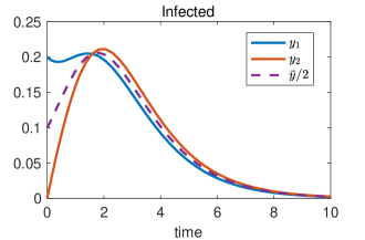
Figure 1: Numerical simulation of the network SIR epidemic model with $n=2$ nodes with interaction matrix $A=\bm{1}\bm{1}^{\prime}$, recovery rate $\gamma=1$, and initial condition $y_{1}(0)=1-x_{1}(0)=0.2$ and $y_{2}(0)=1-x_{2}(0)=0$ satisfying (5)-(6).

Consider the network SIR epidemic model (1) with $n=2$ subpopulations, interaction matrix $A=\bm{1}\bm{1}^{\prime}$, unitary recovery rate $\gamma=1$, and initial condition

$$y_{1}(0)=1-x_{1}(0)=\varepsilon\,,\quad y_{2}(0)=1-x_{2}(0)=0\,,$$ (5)

for some $\varepsilon>0$ is such that

$$\frac{1-\varepsilon}{2-\varepsilon}(1-\log(2-\varepsilon))>\varepsilon\,.$$ (6)

Notice that a range of such values of $\varepsilon$ always exist since the function $g(\varepsilon)=\frac{1-\varepsilon}{2-\varepsilon}(1-\log(2-\varepsilon))-\varepsilon$ is continuous in the interval $[0,1]$ and such that $g(0)=1/2(1-\log 2)>0$.

Observe that with these initial conditions we have

$$\dot{y}_{1}(0)=x_{1}(0)(y_{1}(0)+y_{2}(0))-y_{1}(0)=-\varepsilon^{2}<0\,,$$ (7)

which implies that $y_{1}(t)$ is strictly decreasing for sufficiently small $t>0$. We will now show that $y_{1}(t)$ cannot remain decreasing for all values of $t\geq 0$, but will necessary become increasing in a certain time range, before eventually starting to decrease again and vanish as $t$ grows large.

Towards this goal, first observe that the aggregate variables $\overline{x}=x_{1}+x_{2}$ and $\overline{y}=y_{1}+y_{2}$ satisfy an autonomous scalar SIR epidemic model

$$\dot{\overline{x}}=-\overline{x}\,\overline{y}\,,\qquad\dot{\overline{y}}=(\overline{x}-1)\overline{y}\,.$$ (8)

Then, since $\dot{\overline{y}}(0)=(\overline{x}(0)-1)\overline{y}(0)>0\,,$ Proposition 2.2 (iii) implies that there exists a peak time $\hat{t}>0$ at which $\dot{\bar{y}}(\hat{t}\,)=0$, i.e., $\overline{x}(\hat{t}\,)=1$. This, Proposition 2.2(i) and (5) imply that

$$\overline{y}(\hat{t}\,)=\overline{x}(0)+\overline{y}(0)-\overline{x}(\hat{t}\,)+\log\frac{\overline{x}(\hat{t}\,)}{\overline{x}(0)}\\ =1-\log(2-\varepsilon)\,.$$ (9)

Since $\dot{x}_{2}=-x_{2}\overline{y}$ and $x_{2}(0)=1$, we have that

$$x_{2}(\hat{t}\,)=\exp\Big{(}-\int_{0}^{\hat{t}}\overline{y}(t)\mathrm{d}t\Big{)}=\frac{\overline{x}(\hat{t}\,)}{\overline{x}(0)}=\frac{1}{2-\varepsilon}\,,$$ (10)

where the second equality follows from integrating the first equation in (8) and the last one follows from (5). It then follows from (9) and (10) that

$$\dot{y}_{2}(\hat{t}\,)=x_{2}(\hat{t}\,)\overline{y}(\hat{t}\,)-y_{2}(\hat{t}\,)=\frac{1-\log(2-\varepsilon)}{2-\varepsilon}-y_{2}(\hat{t}\,)\,.$$ (11)

Now, assume by contradiction that $\dot{y}_{1}(t)\leq 0$ for all $t\geq 0$. In particular, this would imply that $y_{1}(\hat{t}\,)\leq y_{1}(0)=\varepsilon$, so that

$$y_{2}(\hat{t}\,)=\overline{y}(\hat{t}\,)-y_{1}(\hat{t}\,)\geq 1-\log(2-\varepsilon)-\varepsilon\,.$$

by (9). Recalling that $\dot{\overline{y}}(\hat{t}\,)=0$, substituting the above in the righthand side of (11), and using (6) we would then get

$$\dot{y}_{1}(\hat{t}\,)=\dot{\overline{y}}(\hat{t}\,)-\dot{y}_{2}(\hat{t}\,)\geq\frac{1-\varepsilon}{2-\varepsilon}\left(1-\log(2-\varepsilon)\right)-\varepsilon>0\,.$$

It then follows that the must exist some values of $t\geq 0$ such that $\dot{y}_{1}(t)>0$. Together with (7) and the fact $\lim_{t\to+\infty}y_{1}(t)=0$ by Proposition 1(vi), this implies that $y_{1}(t)$ has a multimodal behavior.

In fact, the results in Section 3 will imply that such behavior is necessarily as illustrated in Figure 1: $y_{1}(t)$ is strictly decreasing in an interval $[0,\check{t}_{1}]$, until reaching a positive local minimum point $\check{t}_{1}>0$, it is then strictly increasing in an interval $[\check{t}_{1},\hat{t}_{1}]$ until reaching a second peak at some time $\hat{t}_{1}>\check{t}_{1}$, and is eventually strictly decreasing for $t\geq\hat{t}_{1}$.

Somewhat surprisingly, the network SIR epidemic model considered in this example can actually be interpreted as a scalar SIR epidemic model where the population of agents has simply been split into two equally sized subpopulations, which have distinct initial conditions. Specifically, the first population has all the initially infected people while the second population is totally constituted by susceptible individuals. The parameters chosen are such that if the two subpopulations were isolated, the first subpopulation would undertake an exponential decrease to a disease-free state. However, because of the presence of the second subpopulation, the infection can further spread and eventually hit back the first subpopulation that thus suffers a second wave of infection with a second peak (the first one being at time $0$).

In the next section we study the network SIR epidemic model with rank-$1$ interaction matrices and provide results on the changes of monotonicity of the curve of the infected fraction of individuals in each subpopulation. In particular, we show that, for arbitrary rank-$1$ interaction matrices, the number of such changes of monotonicity can never exceed two.

3 The network SIR model with rank-$1$ interaction matrices

In this section, we study the network SIR model in the special case when the interaction matrix $A$ has rank $1$, as per the following equivalent assumption.

Assumption 1

The interaction matrix $A$ satisfies

$$A=ab^{T}\,,$$ (12)

for two vectors $a>\bm{0}$ and $b>\bm{0}$ in $\mathbb{R}^{n}$.

Remark 3.5.

Notice that this case encompasses the one studied in [16] where authors impose the extra condition that $A$ is symmetric.

Let us define the weighted sums of susceptible fraction of individuals

$$\bar{x}=\sum_{j=1}^{n}b_{j}x_{j}\,,$$ (13)

and, respectively, of infected fraction of individuals

$$\bar{y}=\sum_{j=1}^{n}b_{j}y_{j}\,,$$ (14)

across the network. Notice that, for rank-1 interaction matrices $A=ab^{T}$, the network SIR epidemic model’s equations (2) can be rewritten as

$$\dot{x}_{i}=-a_{i}x_{i}\bar{y}\,,$$ (15a)

$$\dot{y}_{i}=a_{i}x_{i}\bar{y}-\gamma y_{i}\,,$$ (15b)

for every $i=1,\ldots,n$. Moreover, let

$$\tilde{x}=\sum_{j=1}^{n}a_{j}b_{j}x_{j}\,,$$ (16)

and

$$w_{i}=\tilde{x}-\gamma-a_{i}\overline{y}\,,$$ (17)

for every $i=1,\ldots,n$.

3.1 Invariants of motion and unimodality in the aggregate

We have the following technical result.

Lemma 3.6.

Consider the rank-$1$ network SIR epidemic model (15a)–(15b). Then,

$$\dot{\overline{x}}=-\overline{y}\tilde{x}\,,$$ (18)

and

$$\dot{\overline{y}}=\overline{y}\left(\tilde{x}-\gamma\right)\,.$$ (19)

Moreover,

$$\ddot{y}_{i}=a_{i}x_{i}\overline{y}w_{i}-\gamma\dot{y}_{i}\,.$$ (20)

for every $i=1,\ldots,n$.

Proof 3.7.

See Appendix 7.

Our next result generalizes Proposition 2.2(i) and determines $n$ invariants of motions for the network SIR epidemic model with rank-$1$ interaction matrix.

Proposition 3.8.

Consider the rank-$1$ network SIR epidemic model (15a)–(15b). Then, for every $i=1,\ldots,n$, the quantity

$$h_{i}(x,y)=a_{i}(\overline{x}+\overline{y})-\gamma\log x_{i}\,,$$

is an invariant of motion.

Proof 3.9.

It follows from (18), (19), and (15a) that

$$\begin{array}[]{rcl}\displaystyle\frac{\mathrm{d}}{\mathrm{d}t}h_{i}(x(t),y(t))&=&\displaystyle a_{i}(\dot{\overline{x}}(t)+\dot{\overline{y}}(t))-\gamma\frac{\dot{x}_{i}(t)}{x_{i}(t)}\\[7.0pt] &=&\displaystyle-a_{i}\gamma\overline{y}(t)+\gamma a_{i}\overline{y}(t)\\[7.0pt] &=&0\,,\end{array}$$

thus implying that $h_{i}(x(t),y(t))$ remains constant along the solutions of the network SIR epidemic model (15a)–(15b).

We can now prove the following result, establishing that, for the network SIR model on rank-1 interaction networks, the weighted sum of the infected fractions of individuals $\overline{y}$ defined in (14) has a unimodal behavior.

Proposition 3.10.

Consider the rank-$1$ network SIR epidemic model (15a)–(15b). Then, for every initial condition $(x(0),y(0))$ such that

$$0\lneq x(0)\leq\bm{1}-y(0)\lneq\bm{1}\,,$$ (21)

we have that:

1. $\tilde{x}(t)$ is strictly decreasing for $t\geq 0$ and

   $$\lim_{t\to+\infty}\tilde{x}(t)<\gamma\,;$$ (22)

2. if

   $$\tilde{x}(0)\leq\gamma\,,$$ (23)

   then $\overline{y}(t)$ is strictly decreasing for $t\geq 0$;

3. if

   $$\tilde{x}(0)>\gamma\,,$$ (24)

   then there exists a peak time $\hat{t}>0$ such that $\overline{y}(t)$ is strictly increasing on $[0,\hat{t}]$ and strictly decreasing on $[\hat{t},+\infty)$.

Proof 3.11.

(i) By taking the derivative of both sides of equation (16) and substituting equation (15a), we get

$$\dot{\tilde{x}}=\sum_{j=1}^{n}a_{j}b_{j}\dot{x}_{j}=-\overline{y}\sum_{j=1}^{n}a_{j}^{2}b_{j}x_{j}\,.$$ (25)

Now, the rightmost inequality in (21) and Proposition 1(v) imply that $y(t)>0$ for every $t>0$, whereas the leftmost inequality in (21) and Proposition 1(iv) imply that there exists some $i$ in $\{1,\ldots,n\}$ such that $x_{i}(t)>0$ for every $t\geq 0$. It then follows from (25) and the assumption that $a>\bm{0}$ and $b>\bm{0}$ that

$$\dot{\tilde{x}}(t)=-\overline{y}(t)\sum_{j=1}^{n}a_{j}^{2}b_{j}x_{j}(t)\leq-a_{i}^{2}b_{i}x_{i}(t)\overline{y}(t)<0\,,$$

for every $t>0$, which implies that $t\mapsto\tilde{x}(t)$ is strictly decreasing for $t\geq 0$. Now, let

$$\tilde{x}(\infty)=\lim_{t\to+\infty}\tilde{x}(t)\,.$$

Clearly, if $\tilde{x}(0)\leq\gamma$, then $\tilde{x}(\infty)<\tilde{x}(0)\leq\gamma$, so that inequality (22) is satisfied. On the other hand, if $\tilde{x}(0)>\gamma$ and $\tilde{x}(\infty)\geq\gamma$, then $\tilde{x}(t)>\gamma$ for every $t\geq 0$, so that, by equation (19),

$$\dot{\overline{y}}(t)=\overline{y}(t)\left(\tilde{x}(t)-\gamma\right)\geq 0\,,\qquad\forall t\geq 0\,.$$

The above would then imply that $t\mapsto\overline{y}(t)$ is nondecreasing for $t\geq 0$, so that

$$\lim_{t\to+\infty}\overline{y}(t)\geq\overline{y}(0)>0\,,$$

thus contradicting Proposition 1(vi). Therefore, also when $\tilde{x}(0)>\gamma$ we must have $\tilde{x}(\infty)<\gamma$, thus completing the proof of point (i) of the claim.

(ii) If $\tilde{x}(0)\leq\gamma$, by point (i) we have that $\tilde{x}(t)<\gamma$ for every $t>0$. Hence, equation (19) implies that

$$\dot{\overline{y}}(t)=\overline{y}(t)\left(\tilde{x}(t)-\gamma\right)<0\,\qquad\forall t>0\,,$$

thus showing that $\overline{y}(t)$ is strictly decreasing for $t\geq 0$.

(iii) If $\tilde{x}(0)>\gamma$, by point (i), $\tilde{x}(t)$ is strictly decreasing for $t\geq 0$ and

$$\lim_{t\to+\infty}\tilde{x}(t)<\gamma\,.$$

Then, there necessarily exits a time $\hat{t}>0$ such that $\tilde{x}(t)>\gamma$ for every $0\leq t<\hat{t}$, $\tilde{x}(\hat{t})=\gamma$, and $\tilde{x}(t)<\gamma$ for every $t>\hat{t}$. It then follows from equation (19) that $t\mapsto\overline{y}(t)$ is strictly increasing for $t$ in $[0,\hat{t}]$ and strictly decreasing for $t$ in $[\hat{t},+\infty)$, thus proving the claim.

Remark 3.12.

The result in [12] suggests a sort of unimodal behavior of the infection curve analogous to the scalar case. In particular, if $\lambda_{\max}([x]A)(\tau)<\gamma$ for some $\tau\geq 0$, then the aggregate curve of infected $v_{max}(\tau)^{T}y(t)$ is monotonically decreasing to 0. Instead, if $\lambda_{\max}([x]A)(0)<\gamma$, then for small times $v_{max}(0)^{T}y(t)$ growa exponentially fast. However, notice how the aggregate index $v_{max}(\tau)^{T}y(t)$ explicitly depends on $x(\tau)$ and is not clear that $v_{max}(0)^{T}y(t)$ is indeed unimodal. In our case study with rank-1 interaction matrices $A=ab^{T}$, the left eigenvector of the $[x]A$ is precisely $b$, so the aggregate is constant in this case and does not depend on the time instant.

3.2 Dynamic behavior of the single populations

Let

$$\hat{t}=\inf\{t\geq 0:\,\tilde{x}(t)\leq\gamma\}\,,$$ (26)

and observe that Proposition 3.10(i) implies that $\hat{t}<+\infty$. Also, for every $i=1,\ldots,n$, let

$$\overline{t}_{i}=\inf\{t\!\geq\!0:\,w_{i}(t)\!\leq\!0\}=\inf\{t\!\geq\!0:\,\tilde{x}(t)\!\leq\!\gamma+a_{i}\overline{y}(t)\}\,,$$ (27)

and notice that

$$\overline{t}_{i}\leq\hat{t}\,,$$ (28)

and $\overline{t}_{i}\leq\overline{t}_{j}$ if and only if $a_{j}\leq a_{i}$. Hence, it is possible to order these time instants from the entries of vector $a$.

We now present the following technical results that will prove useful in deriving our main result.

Lemma 3.13.

Consider the rank-$1$ network SIR epidemic model (15a)–(15b) and every initial condition $(x(0),y(0))$ such that $y(0)\gneq 0$. Then,

1. for every $t\geq 0$,

   $$\dot{w}_{i}(t)<-a_{i}\overline{y}w_{i}(t)\,;$$

2. $w_{i}(t)$ is strictly decreasing for $0\leq t\leq\overline{t}_{i}$;

3. for every $t>\overline{t}_{i}$,

   $$w_{i}(t)<0\,;$$

4. if $\dot{y}_{i}(t)=0$ for some $t\geq\overline{t}_{i}$, then $t$ cannot be a local minimum point of $y_{i}(t)$.

Proof 3.14.

See Appendix 8.

We can now state our main result, characterizing the dynamic behavior of the fraction of infected individuals in the single populations of the network SIR epidemic model with rank-$1$ interaction matrix.

Theorem 3.15.

Consider the rank-$1$ network SIR epidemic model (15a)–(15b). Let $i\in\{1,\ldots,n\}$ be such that $y_{i}(0)>0$. Then,

1. $y_{i}(t)$ admits at most one local minimum time $\check{t}_{i}\geq 0$.

Moreover, if such local minimum time $\check{t}_{i}$ exists,

1. it satisfies

   $$0\leq\check{t}_{i}\leq\overline{t}_{i}\,,$$ (29)

   with $\check{t}_{i}=\overline{t}_{i}=0$ if and only if $w_{i}(0)\leq 0$ and $\dot{y}_{i}(0)>0$;

2. it cannot occur after any stationary local maximum point of $y_{i}(t)$.

Proof 3.16.

If $w_{i}(0)\leq 0$ holds true, then $\overline{t}_{i}=0$ and Lemma 3.13(iv) implies that no stationary point $t\geq 0$ of $y_{i}(t)$ can be a local minimum point. It follows that the only local minimum point of $y_{i}(t)$ can possibly be $\check{t}_{i}=0$ (which is the case if and only if $\dot{y}_{i}(0)>0$). On the other hand, if $w_{i}(0)>0$, then the interior extremum theorem and Lemma 3.13(iv) imply that there cannot be any minimum points of $y_{i}(t)$ in the interval $[\overline{t}_{i},+\infty)$. This proves point (ii).

We are then left with studying local minimum points of $y_{i}(t)$ in the interval $[0,\overline{t}_{i})$. Let $s\geq 0$ be a stationary local maximum point of $y_{i}(t)$, and let $u$ in $(s,\overline{t}_{i})$ be a (necessarily stationary) local minimum point of $y_{i}(t)$. Then, we have that

$$\dot{y}_{i}(s)=\dot{y}_{i}(u)=0\,,$$ (30)

and

$$\ddot{y}_{i}(s)\leq 0\,,\qquad\ddot{y}_{i}(u)\geq 0\,.$$ (31)

Since $y_{i}(t)>0$ for all $t\geq 0$, we have that

$$\begin{array}[]{rcl}0&\geq&\ddot{y}_{i}(s)/y_{i}(s)\\[5.0pt] &=&a_{i}x_{i}(s)\overline{y}(s)w_{i}(s)/y_{i}(s)-\gamma\dot{y}_{i}(s)/y_{i}(s)\\[5.0pt] &=&\gamma w_{i}(s)\\[5.0pt] &>&\gamma w_{i}(u)\\[5.0pt] &=&a_{i}x_{i}(u)\overline{y}(u)w_{i}(u)/y_{i}(u)-\gamma\dot{y}_{i}(u)/y_{i}(u)\\[5.0pt] &=&\ddot{y}_{i}(u)/y_{i}(u)\\[5.0pt] &\geq&0\,,\end{array}$$ (32)

where the first and the last inequalities above follow from (31), the first and the last identities follow from (20), the other two identities from (30) and the fact that, by (15b), $a_{i}x_{i}(t)\bar{y}(t)=\gamma y_{i}(t)$ when $\dot{y}_{i}(t)=0$, and the strict inequality in the middle holds true because of Lemma 3.13(ii). As (32) is a contradiction, this shows that a local minimum point $u<\hat{t}_{i}$ of $y_{i}(t)$ cannot follow any stationary local maximum point $s\geq 0$ of $y_{i}(t)$, thus proving point (iii).

Finally, to prove point (i), assume by contradiction that there exist two distinct local minimum points $r<u$ of $y_{i}(t)$ in the interval $[0,\hat{t})$. Then, there would necessarily exist a local maximum point of $y_{i}(t)$ in the interval $(r,u)$. But, since $s>r\geq 0$, such local maximum point would also be stationary, thus violating point (iii). Therefore, there cannot exist two distinct local minimum points $r<u$ of $y_{i}(t)$ in the interval $[0,\hat{t}_{i})$, thus completing the proof of point (i).

Remark 3.17.

Notice that (29) and (28) imply that, if it exists, the local minimum point of $y_{i}$ cannot occur after the peak of $\bar{y}$.

As a consequence of Theorem 3.15 we get the following result classifying the possible behaviors of the fraction of infected individuals in the single populations of the network SIR epidemic model with rank-$1$ interaction matrix. This classification is based on the study of the sign of two quantities:

$$\dot{y}_{i}(0)=a_{i}x_{i}(0)\overline{y}(0)-\gamma y_{i}(0),\,w_{i}(0)=\tilde{x}(0)-\gamma-a_{i}\overline{y}(0).$$

Theorem 3.18.

Consider the rank-$1$ network SIR epidemic model (15a)–(15b). Then, for every $i=1,\ldots,n$,

1. if

   $$\dot{y}_{i}(0)\leq 0\,,$$ (33)

   and

   $$w_{i}(0)\leq 0\,,$$ (34)

   then $y_{i}(t)$ is strictly decreasing for $t\geq 0$;

2. if

   $$\dot{y}_{i}(0)>0\,,$$ (35)

   or if

   $$\dot{y}_{i}(0)=0\,,$$ (36)

   and

   $$w_{i}(0)>0\,,$$ (37)

   then there exists a peak time $\hat{t}_{i}>0$ such that $y_{i}(t)$ is strictly increasing on $[0,\hat{t}_{i}]$ and strictly decreasing on $[\hat{t}_{i},+\infty)$;

3. if

   $$\dot{y}_{i}(0)<0\,,$$ (38)

   and

   $$w_{i}(0)>0\,,$$ (39)

   then either $y_{i}(t)$ is strictly decreasing for $t\geq 0$ or there exist a local minimum time $\check{t}_{i}$ and a peak time $\hat{t}_{i}$ such that $0<\check{t}_{i}<\hat{t}_{i}$ and $y_{i}(t)$ is strictly decreasing on $[0,\check{t}_{i}]$, strictly increasing on $[\check{t}_{i},\hat{t}_{i}]$, and strictly decreasing on $[\hat{t}_{i},+\infty)$;

Proof 3.19.

(i) If (34) holds true, then $\overline{t}_{i}=0$. On the other hand, (33) and Theorem 3.15(ii) rule out the possibility that there exist any minimum point for $y_{i}(t)$. Therefore, $y_{i}(t)$ is strictly decreasing for $t\geq 0$.

(ii) If condition (35) holds true, then Theorem 3.15(i) implies that $\check{t}_{i}=0$ is the only minimum point of $y_{i}(t)$. On the other hand, if equation (36) and condition (39) both hold true, then it follows from (20) that

$$\ddot{y}_{i}(0)=a_{i}x_{i}(0)\overline{y}(0)w_{i}(0)-\gamma\dot{y}_{i}(0)=\gamma\overline{y}^{2}(0)w_{i}(0)>0\,,$$

(where the second identity follows from the fact that, by (15b), $a_{i}x_{i}(t)\bar{y}(t)=\gamma y_{i}(t)$ when $\dot{y}_{i}(t)=0$) thus implying that also in this case $\check{t}_{i}=0$ is a local minimum point for $y_{i}(t)$.

Since, by Proposition 1(vi),

$$\lim_{t\to+\infty}y_{i}(t)=0<y_{i}(0)\,,$$ (40)

and, by Theorem 3.15(i), $y_{i}(t)$ cannot have another local minimum points besides $\check{t}_{i}=0$, it follows that exists a peak time $\hat{t}_{i}>0$ such that $y_{i}(t)$ is strictly increasing for $t$ in $[0,\hat{t}_{i}]$ and strictly decreasing for $t$ in $[\hat{t}_{i},+\infty)$.

(iii) From condition (38), $0$ is a nonstationary local maximum point of $y_{i}(t)$. Since, by Theorem 3.15(i), $y_{i}(t)$ can have at most one local minimum point, and (40) holds true, it follows that either $y_{i}(t)$ is strictly decreasing for $t\geq 0$ (in case there is no local minimum point) or, if a local minimum point $\check{t}_{i}>0$ exists, then there exists also a peak time $\hat{t}_{i}>\check{t}_{i}$ so that $y_{i}(t)$ is strictly increasing on $[0,\hat{t}_{i}]$ and strictly decreasing on $[\hat{t}_{i},+\infty)$.

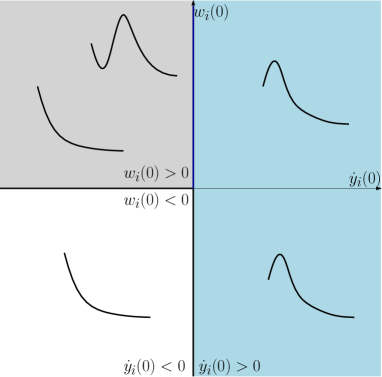
Figure 2: Conceptual illustration of Theorem 3.18.

The previous result provides a classification of the behavior of the fraction of infected individuals in the single populations and in Figure 2 there is a conceptual illustration of this result. In particular, observe that if $\dot{y}_{i}(0)=0$, then the behavior of the single infected fraction depends only on the sign of the quantity $w_{i}(0)$, thus, in this case, the Theorem 3.18 provides a tight condition.

In Theorem 3.18, each condition is considered from the perspective of the individual population $i$. However, note that if (33) is true for all $i=1,\ldots,n$, which means that the infected curve in each population starts decreasing, then no $y_{i}$ will have a local minimum point. Indeed, suppose to multiply both sides of (33) by $b_{i}$ for all $i=1,\ldots,n$ and then sum over all populations, this implies $\tilde{x}(0)<\gamma$ and therefore $w_{i}(0)<0$ for all $i=1,\ldots,n$.

4 Sufficient conditions for multimodal behaviors

We now consider a particular class of rank-1 interaction matrices in the form

$$A=\beta\bm{1}b^{T}\,,$$ (41)

with $\beta>0$ and $\bm{1}^{T}b=1$. This is a special case of the one studied in Section 3 where the vector $a$ has all equal entries and the entries of $b$ sum up to $1$.

Remark 4.20.

This model corresponds to a scenario in which all individuals have the same susceptibility to the disease but different capabilities of spreading the disease. For example, individuals wearing medical masks become infected with the same probability but spread the disease differently. Note that a simple case of this class of matrices is $A=\bm{1}\bm{1}^{\prime}$, that is studied in Example 2.4. The network SIR epidemic model with this interaction matrix is of interest for control applications, as analyzed in [14]. Indeed, even if the dynamics at the nodes are homogeneous and thus the infection spreads at the same rate, it may be convenient to divide agents into multiple groups, for example, to study the effects of differentiated control policies, especially in cases whereby the cost of applying a control and epidemic cost for the diffusion of the disease may differ depending on the age of the agents.

We observe that, for rank-1 interaction matrices in the form (41), the dynamics become

$$\dot{x}_{i}=-\beta x_{i}\bar{y},\qquad\dot{y}_{i}=\beta x_{i}\bar{y}-\gamma y_{i}\,,$$ (42)

for every $i=1,\cdots,n$, and

$$\dot{\overline{x}}=-\beta\overline{x}\,\overline{y},\qquad\dot{\overline{y}}=\overline{y}\left(\beta\overline{x}-\gamma\right)\,,$$ (43)

since $\overline{x}$ and $\tilde{x}$ differ in a constant term only. The next result provides sufficient conditions for multimodal behavior of the infection curve at single node level and encompasses Example 2.4. We first need to define auxiliary functions

$$g_{i}(\varepsilon)=\frac{1-\varepsilon}{1-b_{i}\varepsilon}\left(1-\frac{\gamma}{\beta}+\frac{\gamma}{\beta}\log\frac{\gamma}{\beta(1-b_{i}\varepsilon)}\right)-\varepsilon\,,$$ (44)

Notice that

$$g_{i}(0)=1-\frac{\gamma}{\beta}+\frac{\gamma}{\beta}\log\frac{\gamma}{\beta},\quad g_{i}(1)=-1$$

As a consequence, when $\gamma/\beta<1$, $g_{i}$ admits zeroes in $[0,1]$ and we put

$$\overline{\varepsilon}_{i}=\min\left\{\varepsilon\in[0,1]:\,g_{i}(\varepsilon)=0\right\}.$$ (45)

Proposition 4.21.

Consider the rank $1$ network SIR epidemic model (15a)–(15b) with $a=\beta\bm{1}$ and $\bm{1}^{T}b=1$. Consider an agent $i\in\{1,\ldots,n\}$ and an initial condition $(x(0),y(0))$ that satisfy the following conditions:

$$x(0)+y(0)=\bm{1}$$ (46)

$$\beta x_{i}(0)\bar{y}(0)-\gamma y_{i}(0)<0$$ (47)

$$\beta\overline{x}(0)>\gamma$$ (48)

$$0<y_{i}(0)<\overline{\varepsilon}_{i}$$ (49)

Then, there exist a local minimum time $\check{t}_{i}$ and a peak time $\hat{t}_{i}$ such that $0<\check{t}_{i}<\hat{t}_{i}$ and $y_{i}(t)$ is strictly decreasing on $[0,\check{t}_{i}]$, strictly increasing on $[\check{t}_{i},\hat{t}_{i}]$, and strictly decreasing on $[\hat{t}_{i},+\infty)$.

Proof 4.22.

From (47) and (42) it follows that $\dot{y}_{i}(0)<0$, which implies that $y_{i}(t)$ is strictly decreasing for sufficiently small $t>0$. On the other hand, (43) and (48) imply that $\bar{y}(t)$ is strictly increasing for sufficiently small $t>0$. Since $\overline{x}$ and $\overline{y}$ satisfy the scalar autonomous SIR epidemic model (43), this implies that $\overline{y}(t)$ has a peak at some time $\hat{t}>0$ and

$$\overline{x}(\hat{t})=\frac{\gamma}{\beta}\,.$$ (50)

From Proposition 2.2(i) we obtain that the aggregate peak of infection is

$$\overline{y}(\hat{t}\,) =\overline{x}(0)+\overline{y}(0)-\overline{x}(\hat{t})+\frac{\gamma}{\beta}\log\frac{\overline{x}(\hat{t})}{\overline{x}(0)}$$ (51)

$$=1-\frac{\gamma}{\beta}+\frac{\gamma}{\beta}\log\frac{\gamma}{\beta\overline{x}(0)}\,,$$

where the second equality follows from (46) and (50). Moreover, (42) and (43) imply that

$$\frac{x_{i}(t)}{x_{i}(0)}=\frac{\overline{x}(t)}{\overline{x}(0)}\,,$$ (52)

for every $i=1,\dots,n,$ and every $t$. Therefore, using (50) we obtain

$$x_{i}(\hat{t})=\frac{\gamma}{\beta}\frac{x_{i}(0)}{\overline{x}(0)}\,,$$ (53)

We now prove that $y_{i}(t)$ cannot remain decreasing for all $t>0$. Assume by contradiction that

$$\dot{y}_{i}(t)\leq 0\,,\qquad\forall t\in[0,\hat{t}]\,.$$ (54)

In particular, this implies that $y_{i}(\hat{t})\leq y_{i}(0)$. This together with (53) and (51) imply that

$$\begin{array}[]{rclcl}0&\geq&\dot{y}_{i}(\hat{t}\,)\\[7.0pt] &=&\displaystyle\beta x_{i}(\hat{t}\,)\bar{y}(\hat{t}\,)-\gamma y_{i}(\hat{t}\,)\\[7.0pt] &=&\displaystyle\gamma\frac{x_{i}(0)}{\overline{x}(0)}\left(1-\frac{\gamma}{\beta}+\frac{\gamma}{\beta}\log\frac{\gamma}{\beta\overline{x}(0)}\right)-\gamma y_{i}(\hat{t}\,)\\[9.0pt] &\geq&\displaystyle\gamma\left[\frac{x_{i}(0)}{\overline{x}(0)}\left(1-\frac{\gamma}{\beta}+\frac{\gamma}{\beta}\log\frac{\gamma}{\beta\overline{x}(0)}\right)-y_{i}(0)\right]\end{array}$$ (55)

Notice now that, because of the assumptions on $b$, it holds that $\overline{x}(0)=1-\overline{y}(0)\leq 1-b_{i}y_{i}(0)$. Since the last expression in (55) is decreasing in $\overline{x}(0)$ and $x_{i}(0)=1-y_{i}(0)$, we obtain that

$$0\geq\displaystyle\gamma g_{i}(y_{i}(0))$$ (56)

Notice that by (48), we necessarily have that $\gamma/\beta<1$. This implies that $g_{i}(0)>0$ and, together with (56), implies that $y_{i}(0)\geq\overline{\varepsilon}_{i}$, thus violating (45). This contradiction implies that $y_{i}(t)$ cannot remain decreasing for all $t>0$. The thesis then follows from Theorem 3.18.

Remark 4.23.

Observe that the set of model parameters and initial conditions that satisfy the assumptions of Proposition 4.21 is nonempty. To prove this, let us consider a network with $n$ nodes, interaction matrix as defined in (41) with parameters $\beta>\gamma$ and

$$b_{1}<\min\left\{\frac{\gamma}{\beta},1-\frac{\gamma}{\beta}\right\}\,,$$ (57)

Fix an initial condition such that $y_{1}(0)\in(0,\overline{\epsilon}_{1})$ and $y_{j}(0)=0$ for every $j=2,\cdots,n$. Notice that $\overline{y}(0)=b_{1}y_{1}(0)$. A straightforward check shows that (47) and (48) are automatically satisfied putting no further restriction on $y_{1}(0)$. Therefore, all assumptions of Proposition 4.21 are satisfied.

Remark 4.24.

Observe that under the assumptions of Proposition 4.21 we can provide an upper bound for stationary infection peaks of a node $i$. Let $\hat{t}_{i}$ be the peak time of node $i$, hence $\dot{y}_{i}(\hat{t}_{i})=0$. This implies by (42)

$$y_{i}(\hat{t}_{i})=\frac{\beta x_{i}(\hat{t}_{i})}{\gamma}\overline{y}(\hat{t}_{i})\,.$$ (58)

Since the aggregate quantity of infected is limited above by its infection peak, i.e. $\overline{y}(t)\leq\overline{y}(\hat{t}\,)$, for all $t\geq 0$, and the fraction of susceptibles is monotonically decreasing, then

$$\begin{array}[]{rclcl}y_{i}(\hat{t}_{i})&\leq&\displaystyle\frac{\beta x_{i}(0)}{\gamma}\overline{y}(\hat{t})\\ &=&\displaystyle\frac{\beta x_{i}(0)}{\gamma}\left(\overline{x}(0)+\overline{y}(0)-\overline{x}(\hat{t})+\gamma\log\frac{\overline{x}(\hat{t}\,)}{\overline{x}(0)}\right)\\[9.0pt] &=&\displaystyle x_{i}(0)\left(\frac{\beta}{\gamma}-1+\log\frac{\gamma}{\overline{x}(0)}\right)\,,\\ \end{array}$$

where the first equivalence follows from (51) and the last one from (50) and (46).

5 Numerical Simulations

In this section we provide numerical simulations of the network SIR model. We start by considering a network with $n=5$ nodes and rank-1 interaction matrix. We can observe from Figure 3 that nodes $1$ and $3$ exhibit multimodal behaviors with two changes of monotonicity: for each $i=1,3$, the fraction of infected $y_{i}(t)$ is strictly decreasing for times $t$ in $[0,\check{t}_{i}]$, it is strictly increasing in $[\check{t}_{i},\hat{t}_{i}]$, and it is strictly decreasing for $t$ in $[\hat{t}_{i},+\infty)$. The bottom plot shows the aggregate variable $\overline{y}(t)$, which has a unimodal behavior with a peak in $\hat{t}$, as proved in the Proposition 3.10. Note also that, as consequence of Theorem 3.15(ii) (cfr. Remark 3.17), $\check{t}_{i}\leq\hat{t}$ for every $i=1,3$, namely the local minimum of the infected curve in each node cannot occur after the aggregate infection peak.

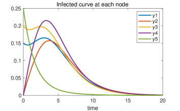
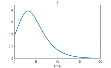
Figure 3: Numerical simulations of the network SIR model on a network with $n=5$ nodes and rank-1 interaction matrix. The interaction matrix is $A=ab^{T}$ with $a=(0.1\,0.25\,0.6\,1\,0.2)$ and $b=(0.45\,0.4\,0.6\,0.65\,0.01)$, and the recovery rate is $\gamma=0.6$. The initial conditions are $x_{1}(0)=0.85$, $x_{2}(0)=0.999$, $x_{3}(0)=0.8$, $x_{4}(0)=1$, $x_{5}(0)=0.75$, and $y(0)=\bm{1}-x(0)$.

Figure 4 illustrates numerical simulations of a network SIR model with $n=2$ and full rank interaction matrix. This simulation shows that dynamics may exhibit more complex behaviors than in the rank $1$ case. In particular, the bottom plot of Figure 4 shows that for suitable initial conditions, the curve of infected in node 1 exhibits two stationary local maxima (with the second higher than the first one) with three changes of monotonicity. We remark that for rank-1 interaction matrices this behavior is ruled out by Theorem 3.15(iii).

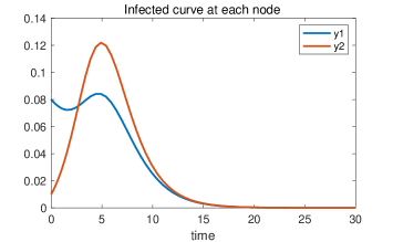
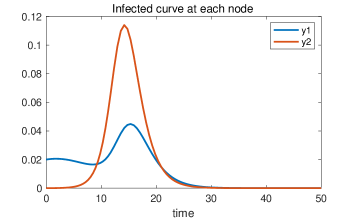
Figure 4: Numerical simulations of the network SIR model on networks with $n=2$ nodes and full rank interaction matrices. In the top plot,
$\displaystyle\hskip 85.35826ptA=\left(\begin{array}[]{cc}0.8&0.5\\ 0.1&1.5\end{array}\right)\,,$
$x_{1}(0)=0.92=1-y_{1}(0)$, $x_{2}(0)=0.99=1-y_{2}(0)$, and $\gamma=0.9$. In the bottom plot,
$\displaystyle\hskip 85.35826ptA=\left(\begin{array}[]{cc}0.95&0.2\\ 0.001&1.6\end{array}\right)\,,$
$x_{1}(0)=0.98=1-y_{1}(0)$, $x_{2}(0)=1=1-y_{2}(0)$, and $\gamma=0.9$.

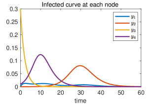
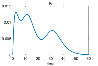
Figure 5: Numerical simulation of the network SIR epidemic model with $n=4$ nodes, recovery rate $\gamma=0.5$, and interaction matrix
$\displaystyle\hskip 28.45274ptA=\left(\begin{array}[]{cccc}0.05&0.05&0.05&0.05\\ 0.0001&0.8&0.0001&0.0001\\ 0.0001&0.0001&0.05&0.0001\\ 0.0009&0.0009&0.0009&0.9\end{array}\right)\,.$
Initial conditions are $x_{1}(0)=x_{2}(0)=1$, $y_{1}(0)=y_{2}(0)=0$, $x_{3}(0)=0.7=1-y_{3}(0)$, $x_{4}(0)=0.99=1-y_{4}(0)$. It can be observed that the curve of infected individuals in the first node has three peaks.

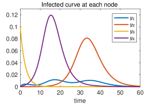
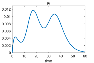
Figure 6: Numerical simulation of the network SIR epidemic model with $n=4$ nodes, recovery rate $\gamma=0.5$, and interaction matrix
$\displaystyle\hskip 28.45274ptA=\left(\begin{array}[]{cccc}0.05&0.07&0.05&0.05\\ 0.0001&0.8&0.0001&0.0001\\ 0.0001&0.0001&0.1&0.0001\\ 0.01&0.01&0.01&0.9\end{array}\right)\,.$
Initial conditions are $x_{1}(0)=x_{2}(0)=x_{4}(0)=1$, $y_{1}(0)=y_{2}(0)=y_{4}(0)=0$, $x_{3}(0)=0.9=1-y_{3}(0)$. It can be observed that the curve of infected individuals in the first subpopulation has three peaks, and the second peak is the highest one.

In Figure 5 we illustrate a numerical simulation of a network SIR model with $n=4$ nodes, where the curves of infected at single node level exhibit three peaks. Moreover, we observe the presence of delays among the peaks in different nodes. Such simulations show that the limitation of the number of peaks to two is a peculiar feature of rank $1$ matrices while for general network matrices, even in correspondence of a limited number of nodes, such limitation does no longer hold. It is also important to note that successive infection peaks can also be greater than the previous one, as observed in Figure 6. This is an interesting phenomenon especially in the design of a control, as an epidemic process is simulated in which after one peak of infection a second larger one may occur.

6 Conclusion

In this paper, we studied the network epidemic SIR model and provided theoretical results on the dynamics for the special case of rank 1 interaction matrices, which finds applications in epidemics control, as shown in [14]. We first proved that, in contrast to the scalar SIR model, in the network SIR model the curve of infected individuals in a single node may exhibit multimodal behaviors, and established sufficient conditions for the occurrence of this phenomenon. We then provided a linear combination of the fraction of infected in each node that exhibits a unimodal behavior, and characterized all the possible behaviors that the dynamics may exhibit at single node level, showing that the infection curve in a single node can undergo two changes of monotonicity at most. We then conducted a numerical analysis showing that for more general interaction matrices the network SIR model may exhibit more than two peaks at single node level. Future work aims to include in the model more complex phenomena, such as waving immunity and endogenous response of agents in response to the disease, to fully describe the occurrence of multimodal behaviors in epidemic models.

7 Proof of Lemma 3.6

By taking the derivative of both sides of (13) and substituting (15a), we get

$$\dot{\overline{x}}=\sum_{j=1}^{n}b_{j}\dot{x}_{j}=-\bar{y}\sum_{j=1}^{n}b_{j}a_{j}x_{j}=-\overline{y}\tilde{x}\,,$$

thus proving (18). Analogously, by taking the derivative of both sides of (14) and substituting (15b), we get

$$\dot{\overline{y}}=\sum_{j=1}^{n}b_{j}\dot{y}_{j}=\bar{y}\sum_{j=1}^{n}b_{j}a_{j}x_{j}-\gamma\overline{y}=\overline{y}\left(\tilde{x}-\gamma\right)\,,$$

thus proving (19). On the other hand, taking the derivative of both sides of (15b) and substituting (15a) and (19) yield

$$\begin{array}[]{rcl}\ddot{y}_{i}&=&a_{i}\left(\dot{x}_{i}\bar{y}+x_{i}\dot{\bar{y}}\right)-\gamma\dot{y}_{i}\\[3.0pt] &=&a_{i}x_{i}\overline{y}\left(\tilde{x}-\gamma-a_{i}\overline{y}\right)-\gamma\dot{y}_{i}\\[3.0pt] &=&a_{i}x_{i}\overline{y}w_{i}-\gamma\dot{y}_{i}\,,\end{array}$$

thus proving (20).

8 Proof of Lemma 3.13

(i) From (15a), we have that

$$\dot{\tilde{x}}=\sum_{i}a_{i}b_{i}\dot{x}_{i}=-\overline{y}\sum_{i}a_{i}^{2}b_{i}x_{i}\leq 0\,.$$ (59)

On the other hand, thanks to Proposition 1(v), the assumption that $y(0)\gneq 0$ implies that

$$y(t)>0\,,\qquad\forall t>0\,,$$ (60)

so that in particular

$$\overline{y}(t)=\sum_{j}b_{j}y_{j}(t)>0\,,\qquad\forall t\geq 0\,.$$ (61)

It then follows from (17),(19), (59), and (61) that

$$\dot{w}_{i}=\dot{\tilde{x}}-a_{i}\dot{\overline{y}}=\dot{\tilde{x}}-a_{i}\overline{y}(\tilde{x}-\gamma)=\dot{\tilde{x}}-a_{i}\overline{y}w_{i}-a_{i}^{2}\overline{y}^{2}<-a_{i}\overline{y}w_{i}\,,$$

thus proving the claim.

(ii) For $0\leq t\leq\overline{t}_{i}$, we have $w_{i}(t)\geq 0$ so that, by point (i) and (61), we have that

$$\dot{w}_{i}(t)<-a_{i}\overline{y}(t)w_{i}(t)\leq 0\,.$$

The above implies that $w_{i}(t)$ is strictly decreasing for $0\leq t\leq\overline{t}_{i}$.

(iii) It follows from point (i) that, for every $t_{i}^{*}\geq 0$ such that $w_{i}(t_{i}^{*})=0$, we have

$$\dot{w}_{i}(t_{i}^{*})<-a_{i}\overline{y}(t_{i}^{*})w_{i}(t_{i}^{*})=0\,,$$

so that $w_{i}(t)<0$ for $t>t_{i}^{*}$. If $w_{i}(0)\leq 0$ so that $\overline{t}_{i}=0$, the above implies that $w_{i}(t)<0$ for every $t>0=\overline{t}_{i}$. On the other hand, $w_{i}(0)>0$ so that $\overline{t}_{i}>0$, the above implies that $w_{i}(t)<0$ for every $t>\overline{t}_{i}$.

(iv) Assume by contradiction that $t\geq\overline{t}_{i}$ is a local minimum point of $y_{i}(t)$ with $\dot{y}_{i}(t)=0$. By (20), we then have

$$\ddot{y}_{i}(t)=a_{i}x_{i}(t)\overline{y}(t)w_{i}(t)-\gamma\dot{y}_{i}(t)\\ =\gamma y_{i}(t)w_{i}(t)\,,$$ (62)

where the last identity holds true since, by (15b), $\dot{y}_{i}(t)=0$ is equivalent to

$$a_{i}x_{i}(t)\bar{y}(t)=\gamma y_{i}(t)\,.$$ (63)

Equation (62) and (60) imply that

$$\operatorname{sgn}(\ddot{y}_{i}(t))=\operatorname{sgn}(w_{i}(t))\,.$$ (64)

Now, recall that by point (iii) we have $w_{i}(t)\leq 0$ for every $t\geq\overline{t}_{i}$. If $w_{i}(t)<0$, then equation (64) implies that $\ddot{y}_{i}(t)<0$, so that $t$ cannot be a local minimum point for $y_{i}(t)$. On the other hand, if $w_{i}(t)=0$, by point (i) and (61) we get that

$$\dot{w}_{i}(t)<-a_{i}\overline{y}(t)w_{i}(t)=0\,,$$ (65)

while equation (64) implies that $\ddot{y}_{i}(t)=0$. Hence, by taking the derivative of both sides of (20), by (63) and $w_{i}(t)=0$, we get

$$\begin{array}[]{rcl}\dddot{y}_{i}(t)&=&a_{i}x_{i}(t)\overline{y}(t)\dot{w}_{i}(t)+a_{i}(\dot{(x_{i}(t)\overline{y}(t))})w_{i}(t)-\gamma\ddot{y}_{i}(t)\\[5.0pt] &=&\gamma y_{i}(t)\dot{w}_{i}(t)\\[5.0pt] &<&0\,,\end{array}$$

where the last inequality following from (60) and (65). Together with $\dot{y}_{i}(t)=\ddot{y}_{i}(t)=0$, the above implies that $t$ is an inflection point for $y_{i}(t)$, hence it particular it is not a local minimum point. We have thus proven that $y_{i}(t)$ cannot have any stationary minimum points in the interval $[\overline{t}_{i},+\infty)$.

[]Martina Alutto received the B.Sc. in Mathematics for Engineering in 2018 from Politecnico di Torino, Italy, the M.S. in Mathematical Engineering (cum Laude) in 2021 from Politecnico of Turin, Italy. She is currently a PhD student in Pure and Applied mathematics at the Department of Mathematical Sciences, Politecnico di Torino, Italy. Her research interests focuses on analysis and control of network systems, with application to epidemics and social networks.

[]Leonardo Cianfanelli received the B.Sc. (cum Laude) in Physics and Astrophysics in 2014 from Università  degli Studi di Firenze, Italy, the M.S. in Physics of Complex Systems (cum Laude) in 2017 from Università di Torino, Italy, and the PhD in Pure and Applied Mathematics in 2022 from Politecnico di Torino. He is currently a Research Assistant at the Department of Mathematical Sciences, Politecnico di Torino, Italy. He was a Visiting Student at Laboratory for Information and Decision Systems, Massachusetts Institute of Technology, in 2018-2020. His research focuses on control in network systems, with applications to transportation networks and epidemics.

[] Giacomo Como(M’12) is a Professor at the Department of Mathematical Sciences, Politecnico di Torino, Italy. He is also a Senior Lecturer at the Automatic Control Department, Lund University, Sweden. He received the B.Sc., M.S., and Ph.D. degrees in Applied Mathematics from Politecnico di Torino, in 2002, 2004, and 2008, respectively. He was a Visiting Assistant in Research at Yale University in 2006–2007 and a Postdoctoral Associate at the Laboratory for Information and Decision Systems, Massachusetts Institute of Technology in 2008–2011. Prof. Como currently serves as Senior Editor for the IEEE Transactions on Control of Network Systems, as Associate Editor for Automatica, and as the chair of the IEEE-CSS Technical Committee on Networks and Communications. He served as Associate Editor for the IEEE Transactions on Network Science and Engineering (2015-2021) and for the IEEE Transactions on Control of Network Systems (2016-2022). He was the IPC chair of the IFAC Workshop NecSys’15 and a semiplenary speaker at the International Symposium MTNS’16. He is recipient of the 2015 George S.  Axelby Outstanding Paper Award. His research interests are in dynamics, information, and control in network systems, with applications to infrastructure, social, and economic networks.

[] Fabio Fagnani received the Laurea degree in Mathematics from the University of Pisa and the Scuola Normale Superiore, Pisa, Italy, in 1986. He received the PhD degree in Mathematics from the University of Groningen, Groningen, The Netherlands, in 1991. From 1991 to 1998, he was an Assistant Professor at the Scuola Normale Superiore. In 1997, he was a Visiting Professor at the Massachusetts Institute of Technology. Since 1998, he has been with the Politecnico of Torino, where since 2002 he has been a Full Professor. From 2006 to 2012, he has acted as Coordinator of the PhD program in Mathematics for Engineering Sciences at Politecnico di Torino. From 2012 to 2019, he served as the Head of the Department of Mathematical Sciences, Politecnico di Torino. His current research focuses on dynamical systems over graphs, inferential distributed algorithms, and opinion dynamics. He is an Associate Editor of the IEEE Transactions on Automatic Control and served in the same role for the IEEE Transactions on Network Science and Engineering and of the IEEE Transactions on Control of Network Systems.

References

- [1] M. Alutto, L. Cianfanelli, G. Como, and F. Fagnani. Multiple peaks in network sir epidemic models. In 2022 IEEE 61st Conference on Decision and Control (CDC), pages 5614–5619, 2022.
- [2] W. O. Kermack and A. G. McKendrick. A contribution to the mathematical theory of epidemics. Proceedings of the Royal Society of London. Series A, 115(772):700–721, 1927.
- [3] H. W. Hethcote. The mathematics of infectious diseases. SIAM Rev., 42:599–653, 2000.
- [4] A. G. McKendrick. Applications of mathematics to medical problems. Proceedings of the Edinburgh Mathematical Society, 44:98 – 130.
- [5] Odo Diekmann and J. A. P. Heesterbeek. Mathematical epidemiology of infectious diseases: Model building, analysis and interpretation. 2000.
- [6] M. Alutto, G. Como, and F. Fagnani. On sir epidemic models with feedback-controlled interactions and network effects. 2021 60th IEEE Conference on Decision and Control (CDC 2021), pages 5562–5567, 2021.
- [7] L. Cianfanelli, F. Parise, D. Acemoglu, G. Como, and A. Ozdaglar. Lockdown interventions in the SIR model: Is the reproduction number the right control variable? In Proceedings of the 60th IEEE Conference on Decision and Control (CDC 2021), pages 4254–4259. IEEE, 2021.
- [8] L. Miclo, D. Spiro, and J. Weibull. Optimal epidemic suppression under an ICU constraint. Journal of Mathematical Economics, 101:102669, 2022.
- [9] H. W Hethcote. An immunization model for a heterogeneous population. Theoretical population biology, 14(3):338–349, 1978.
- [10] A. Fall, A. Iggidr, G. Sallet, and J. J. Tewa. Epidemiological models and lyapunov functions. Math. Model. Nat. Phenom., 2(1):62–83, 2007.
- [11] C. Nowzari, V. M. Preciado, and G. J. Pappas. Analysis and control of epidemics: A survey of spreading processes on complex networks. IEEE Control Systems Magazine, 36(1):26–46, 2016.
- [12] W. Mei, S. Mohagheghi, S. Zampieri, and F. Bullo. On the dynamics of deterministic epidemic propagation over networks. Annual Reviews in Control, 44:116–128, 2017.
- [13] M. Ogura and V. M. Preciado. Stability of spreading processes over time-varying large-scale networks. IEEE Transactions on Network Science and Engineering, 3:44–57, 2016.
- [14] D. Acemoglu, V. Chernozhukov, I. Werning, and M. D Whinston. Optimal targeted lockdowns in a multigroup sir model. American Economic Review: Insights, 3(4):487–502, 2021.
- [15] A. A. Rampini. Sequential lifting of covid-19 interventions with population heterogeneity. Working Paper 27063, National Bureau of Economic Research, April 2020.
- [16] G. Ellison. Implications of heterogeneous sir models for analyses of covid-19. Working Paper 27373, National Bureau of Economic Research, June 2020.
- [17] M. Ehrhardt, J. Gašper, and S. Kilianová. Sir-based mathematical modeling of infectious diseases with vaccination and waning immunity. Journal of Computational Science, 37, 08 2019.
- [18] V. Capasso and G. Serio. A generalization of the kermack-mckendrick deterministic epidemic model. Mathematical Biosciences, 42(1):43–61, 1978.
- [19] Y. Jin, W. Wang, and S. Xiao. An sirs model with a nonlinear incidence rate. Chaos, Solitons & Fractals, 34:1482–1497, 12 2007.
- [20] C. Li, C. Tsai, and S. Yang. Analysis of epidemic spreading of an sirs model in complex heterogeneous networks. Communications in Nonlinear Science and Numerical Simulations, 19:1042–1054, 04 2014.
- [21] M. Li and J. Muldowney. Global stability for the seir model in epidemiology. Mathematical biosciences, 125:155–64, 03 1995.
- [22] G. Giordano, F. Blanchini, R. Bruno, P. Colaneri, A. Di Filippo, A. Di Matteo, and M. Colaneri. Modelling the COVID-19 epidemic and implementation of population-wide interventions in italy. Nature Medicine, 26(6):855–860, apr 2020.
- [23] J. R. Birge, O. Candogan, and Y. Feng. Controlling epidemic spread: reducing economic losses with targeted closures. University of Chicago, Becker Friedman Institute for Economics Working Paper, (2020-57), 2020.
- [24] F. Parino, L. Zino, M. Porfiri, and A. Rizzo. Modelling and predicting the effect of social distancing and travel restrictions on covid-19 spreading. Journal of the Royal Society Interface, 18(175):20200875, 2021.
- [25] F. Brauer, C. Castillo-Chavez, and Z. Feng. Mathematical models in epidemiology. Texts in Applied Mathematics, 2019.