Quantum Equipartition Theorem for Arbitrary Quadratic Systems

Abstract

Equipartition theorem is a fundamental law of classical statistical physics, which states that every degree of freedom contributes $k_{B}T/2$ to the energy, where $T$ is the temperature and $k_{B}$ is the Boltzmann constant. However, a general quantum analogue of equipartition theorem has never been put forward yet. In the present Letter, we focus on how to obtain generalized equipartition theorem for arbitrary quadratic systems where the multimode Brownian ocillators interacts with multiple reservoirs at the same temperature. An alternative method of deriving the energy of the system is also discussed and compared with the result of the equipartition theorem, after which we conclude that the latter is more reasonable. Our results can be viewed as an indispensable generalization of rencent works on quantum equipartition theorem.

Introduction.— One of the elegant principles of classical statistical physics is the equipartition theorem, which has numerous applications in various topics, such as thermodynamics [1, 2, 3], astrophysics [4, 5, 6] and applied physics [7, 8, 9]. Though quantum mechanics has been founded over a hundred years and so as quantum statistical mechanics, there is still no general quantum version of the equipartition theorem.

Recent years have seen much progress on this topic. A novel work [10] investigated the simplest quantum Brownian oscillator model to formulate the energy of the system in terms of the averge energy of a quantum oscillator in a harmonic well. Based on this work, more papers [11, 12, 13, 14, 15, 16, 17, 18] tried to study quantum equipartition theorem in different versions of quadratic open quantum systems from various perspectives, including electrical circuits [11] and dissipative diamagnetism [18].

In this Letter, we aim to deduce the generalized equipartition theorem for arbitray open quantum quadratic systems. Many quadratic systems share the same algebra $[\hat{A},\hat{B}]=i\hbar$, where the binary operator pair can be the coordinate $\hat{x}$ and the momentum $\hat{p}$ for oscillators, the magnetic flux $\hat{\Phi}$ and charge $\hat{Q}$ for quantum circuits, and so on. We here turn to Brownian oscillators as an example to grasp the physical nature of all these systems. It is worth noting [19] that linearly coupled driven Brownian oscillator systems share the same exact dynamical process as undriven systems, as long as we absorb the external field $\epsilon(t)$ into the stochastic force of the bath. We thus only consider undriven systems for simplicity.

To construct such systems, we adopt a generalized Calderia-Leggett model [20] and manage to transform it into a multi-mode Brownian oscillator system well-discussed in Ref. [21]. For generality, we do not choose a concrete form of dissipation. We also generalize a formula [22] for the internal energy so that it could be applied to the multi-mode Brownian oscillator system. It has been debated [23] which of this formula or the quantum equipartition theorem given in  Ref. [10] truly describes the energy of the system. Our analysis show that the generalized version of the former formula cannot be used to find the energy, which implies that the latter one is more reasonable.

Arbitrary quadratic system.— To construct our arbitrary quadratic system, let us start with the multi-mode Calderia-Leggett model [20]

$$H_{\mbox{\tiny CL}} =\sum_{u}\frac{\hat{P}^{2}_{u}}{2M_{u}}+\sum_{uv}\frac{1}{2}k_{uv}\hat{Q}_{u}\hat{Q}_{v}+\sum_{\alpha j}\bigg{[}\frac{\hat{p}^{2}_{\alpha j}}{2m_{\alpha j}}$$

$$\quad\quad+\frac{1}{2}m_{\alpha j}\omega^{2}_{\alpha j}\bigg{(}\hat{x}_{\alpha j}+\frac{1}{m_{\alpha j}\omega^{2}_{\alpha j}}\sum_{u}c_{\alpha uj}\hat{Q}_{u}\bigg{)}^{2}\bigg{]},$$ (1)

where $u,v\in\{1,2,...,n_{\mbox{\tiny S}}\}$ and $j\in\{1,2,...,n_{\alpha}\}$ are indices for the oscillators in the system and in the $\alpha$th bath, repectively. The coefficient $c_{\alpha uj}$ represents the coupling strength between the coordinate of the $u$th oscillator in the system and the $j$th oscillator in the $\alpha$th bath. The convention would put $-c_{\alpha uj}$ in the last term of Eq. (Quantum Equipartition Theorem for Arbitrary Quadratic Systems), but we replace it by $c_{\alpha uj}$. We also have the commutation relations for all the momentum and position operators as follows:

$$[\hat{Q}_{u},\hat{P}_{v}]=i\delta_{uv},\quad[\hat{x}_{\alpha_{1}j_{1}},\hat{p}_{\alpha_{2}j_{2}}]=i\delta_{\alpha_{1}\alpha_{2}}\delta_{j_{1}j_{2}}$$ (2)

with $\delta$ representing the Kronecker delta. Equation (Quantum Equipartition Theorem for Arbitrary Quadratic Systems) can be reorganized in the following forms:

$$H_{\mbox{\tiny CL}}=H_{\mbox{\tiny S}}+H_{\mbox{\tiny S}\mbox{\tiny B}}+h_{\mbox{\tiny B}},$$ (3a)

$$H_{\mbox{\tiny S}}=\sum_{u}\frac{\hat{P}^{2}_{u}}{2M_{u}}+\frac{1}{2}\sum_{uv}k_{uv}\hat{Q}_{u}\hat{Q}_{v},$$ (3b)

$$H_{\mbox{\tiny S}\mbox{\tiny B}}=\sum_{\alpha u}\hat{Q}_{u}\hat{F}_{\alpha u}+\frac{1}{2}\sum_{\alpha j}\frac{c_{\alpha uj}c_{\alpha vj}}{m_{\alpha j}\omega^{2}_{\alpha j}}\hat{Q}_{u}\hat{Q}_{v},$$

$$\quad\hat{F}_{\alpha u}=\sum_{j}c_{\alpha uj}\hat{x}_{\alpha j},$$ (3c)

$$h_{\mbox{\tiny B}}=\sum_{\alpha}h_{\alpha\mbox{\tiny B}}=\sum_{\alpha j}\bigg{(}\frac{\hat{p}^{2}_{\alpha j}}{2m_{\alpha j}}+\frac{1}{2}m_{\alpha j}\omega^{2}_{\alpha j}\hat{x}^{2}_{\alpha j}\bigg{)}.$$ (3d)

Here, the system-bath interaction results from the linear coupling of the system coordinate $\hat{Q}_{u}$ and the random force $\hat{F}_{\alpha u}$. We also emphasize that all the mutually independent baths $\{h_{\alpha\mbox{\tiny B}}\}$ in Eq. (3d) are at the same temperature $\beta$. By defining the pure bath response function as

$$\bm{\phi}_{\alpha}(t)\equiv\{\phi_{\alpha uv}(t)\equiv i\langle[\hat{F}^{\mbox{\tiny B}}_{\alpha u}(t),\hat{F}^{\mbox{\tiny B}}_{\alpha v}(0)]\rangle_{\mbox{\tiny B}}\},$$ (4)

we recognize that

$$\sum_{\alpha j}\frac{c_{\alpha uj}c_{\alpha vj}}{m_{\alpha j}\omega^{2}_{\alpha j}}=\tilde{\phi}_{\alpha uv}(0),$$ (5)

where $\hat{F}^{\mbox{\tiny B}}_{\alpha u}(t)\equiv e^{ih_{\mbox{\tiny B}}t}\hat{F}_{\alpha u}e^{-ih_{\mbox{\tiny B}}t}$ and the average is defined over the canonical ensembles of baths as in $\langle\cdots\rangle_{\mbox{\tiny B}}\equiv\text{tr}_{\mbox{\tiny B}}[\cdots\,\otimes_{\alpha}e^{-\beta h_{\alpha\mbox{\tiny B}}}]/\prod_{\alpha}\text{tr}_{\mbox{\tiny B}}(e^{-\beta h_{\alpha\mbox{\tiny B}}})$. In Eq. (5) we use tilde to denote the Laplace transform $\tilde{f}(\omega)=\int_{0}^{\infty}\mathrm{d}\omega\,e^{i\omega t}f(t)$ for any function $f(t)$. If we denote $V_{uv}\equiv k_{uv}+\sum_{\alpha}\tilde{\phi}_{\alpha uv}(0)$ and $\Omega_{u}\equiv M^{-1}_{u}$ for convenience, then Eqs. (3b) and (3) can be rewritten in the form:

$$H_{\mbox{\tiny S}}+H_{\mbox{\tiny S}\mbox{\tiny B}}$$

$$\equiv\bigg{[}\frac{1}{2}\sum_{u}\Omega_{u}\hat{P}^{2}_{u}+\frac{1}{2}\sum_{uv}\Big{(}V_{uv}-\sum_{\alpha}\tilde{\phi}_{\alpha uv}(0)\Big{)}\hat{Q}_{u}\hat{Q}_{v}\bigg{]}$$

$$\quad+\bigg{[}\sum_{\alpha u}\hat{Q}_{u}\hat{F}_{\alpha u}+\frac{1}{2}\sum_{\alpha uv}\tilde{\phi}_{\alpha uv}(0)\hat{Q}_{u}\hat{Q}_{v}\bigg{]},$$ (6)

which is the starting point of our quantum equipartition theorem. The total Hamiltonian, referred to as [cf. Eq. (3)], now remains identical to the one presented in  Ref. [21]. Physically, we need $\bm{V}=\{V_{uv}\}$, $\bm{k}=\{k_{uv}\}$ and $\bm{\Omega}=\{\Omega_{u}\delta_{uv}\}$ to be positive definite. Detailed derivation of Eq. (5) can be found in  Ref. [24].

Generalizad equipartition theorem.— The conventional equipartition theorem deals with the kinetic energy and the potential energy separately contributed by certain degrees of freedom [10]. When some degrees of freedom are interwined with each other, such as in our model [cf. Eqs. (3, 3b, 3d)], we would better discuss the generalized equipartition theorem [25]. In the rest of this work we study the quantity $\langle\hat{X}_{i}\partial H_{\mbox{\tiny S}}/\partial\hat{X}_{j}\rangle$ for any system degrees of freedom $\hat{X}_{i},\hat{X}_{j}\in\{\hat{P}_{u}\}\cup\{\hat{Q}_{u}\}$. We focus on the cases $i=j$ in the main text. Other cases are discussed in  Ref. [24].

We have $\langle\hat{Q}_{u}\partial H_{\mbox{\tiny S}}/\partial\hat{Q}_{u}\rangle=\sum_{v}[V_{uv}-\sum_{\alpha}\tilde{\phi}_{\alpha uv}(0)]\langle\hat{Q}_{u}\hat{Q}_{v}\rangle$ when we choose $\hat{X}_{i}=\hat{Q}_{u}$. Here, the angular brackets denote the average over the steady state of the total composite system $\rho^{\rm st}_{\mbox{\tiny T}}$, whose partial trace of bath is the system equilibrium state: $\rho_{\mbox{\tiny S}}:=\operatorname{tr}_{\mbox{\tiny B}}\rho^{\rm st}_{\mbox{\tiny T}}=e^{-\beta H_{\mbox{\tiny S}}}/\operatorname{tr}_{\mbox{\tiny S}}e^{-\beta H_{\mbox{\tiny S}}}$. Under the help of the fluctuation-disspation theorem [26], we obtain

$$\bigg{\langle}\hat{Q}_{u}\frac{\partial H_{\mbox{\tiny S}}}{\partial\hat{Q}_{u}}\bigg{\rangle} =\sum_{v}\frac{1}{\pi}\int_{0}^{\infty}\mathrm{d}\omega\,\bigg{[}V_{uv}$$

$$\quad-\sum_{\alpha}\tilde{\phi}_{\alpha uv}(0)\bigg{]}J^{QQ}_{uv}(\omega)\coth\frac{\beta\omega}{2},$$ (7)

with $\bm{J}^{QQ}(\omega)=\{J^{QQ}_{uv}(\omega)\}$ being the anti–Hermitian part of the matrix $\tilde{\bm{\chi}}^{QQ}(\omega)=\{\tilde{\chi}^{QQ}_{uv}(\omega)=\int_{0}^{\infty}\mathrm{d}\omega\,e^{i\omega t}\chi^{QQ}_{uv}(t)\}$. Here, we denote the system response function of any two operators $\hat{A}_{u}$ and $\hat{B}_{v}$ as $\chi^{AB}_{uv}(t)\equiv i\langle[\hat{A}_{u}(t),\hat{B}_{v}(0)]\rangle$. According to  Ref. [21], we also have an explicit expression for $\tilde{\bm{\chi}}^{QQ}(\omega)$ in the form of

$$\tilde{\bm{\chi}}^{QQ}(\omega)=\Big{[}\bm{\Omega}\bm{V}-\omega^{2}\mathbf{I}-\bm{\Omega}\sum_{\alpha}\tilde{\bm{\phi}}_{\alpha}(\omega)\Big{]}^{-1}\bm{\Omega},$$ (8)

where $\bm{V}$ and $\bm{\Omega}$ are given below Eq. (Quantum Equipartition Theorem for Arbitrary Quadratic Systems). Equation (Quantum Equipartition Theorem for Arbitrary Quadratic Systems) can be recast as

$$\bigg{\langle}\hat{Q}_{u}\frac{\partial H_{\mbox{\tiny S}}}{\partial\hat{Q}_{u}}\bigg{\rangle}=\int_{0}^{\infty}\mathrm{d}\omega\,\mathbb{P}^{Q}_{u}(\omega)\bigg{\langle}\hat{Q}_{u}\frac{\partial H_{\mbox{\tiny S}}}{\partial\hat{Q}_{u}}\bigg{\rangle}_{\rm c}(\omega,\beta),$$ (9)

where

$$\bigg{\langle}\hat{Q}_{u}\frac{\partial H_{\mbox{\tiny S}}}{\partial\hat{Q}_{u}}\bigg{\rangle}_{\rm c}(\omega,\beta)=\frac{\omega}{2}\coth\frac{\beta\omega}{2}$$ (10)

and

$$\mathbb{P}^{Q}_{u}(\omega)=\frac{2}{\pi\omega}\sum_{v}\bigg{[}V_{uv}-\sum_{\alpha}\tilde{\phi}_{\alpha uv}(0)\bigg{]}J_{uv}(\omega).$$ (11)

In Eq. (10) the subscript “c” denotes the canonical ensemble averge of a closed system with $c_{\alpha uj}=0$ and $\bm{V}=\omega^{2}\bm{\Omega}^{-1}$ in Eq. (3). The closed system here is a set of noninteracting harmonic oscillators with the same frequencies $\omega$. Therefore, the left-hand side of Eq. (10) equals twice the average potential energy of a harmonic oscillator in the canonical ensemble, which is well known to be $(\omega/2)\coth(\beta\omega/2)$. A similar process for the case $\hat{X}=\hat{P}_{u}$ leads to $\langle\hat{P}_{u}\partial H_{\mbox{\tiny S}}/\partial\hat{P}_{u}\rangle=\Omega_{u}\langle\hat{P}^{2}_{u}\rangle$. Using the fluctuation-dissipation theorem [26] again, we find

$$\bigg{\langle}\hat{P}_{u}\frac{\partial H_{\mbox{\tiny S}}}{\partial\hat{P}_{u}}\bigg{\rangle} =\frac{\Omega_{u}}{\pi}\int_{0}^{\infty}\mathrm{d}\omega\,J^{PP}_{uu}(\omega)\coth\frac{\beta\omega}{2}.$$ (12)

where $\bm{J}^{PP}(\omega)=\{J^{PP}_{uv}(\omega)\}$ is the anti-Hermitian part of matrix $\tilde{\bm{\chi}}^{PP}(\omega)=\{\tilde{\chi}^{PP}_{uv}(\omega)\}$[21]:

$$\tilde{\bm{\chi}}^{PP}(\omega)=\bm{\Omega}^{-1}+\omega^{2}\bm{\Omega}^{-1}\tilde{\bm{\chi}}^{QQ}(\omega)\bm{\Omega}^{-1}.$$ (13)

We obtain

$$\bigg{\langle}\hat{P}_{u}\frac{\partial H_{\mbox{\tiny S}}}{\partial\hat{P}_{u}}\bigg{\rangle}_{\rm c}(\omega,\beta)=\frac{\omega}{2}\coth\frac{\beta\omega}{2},$$ (14)

for the same closed system with $c_{\alpha uj}=0$ and $\bm{V}=\omega^{2}\bm{\Omega}^{-1}$. It is evident that the left-hand side of Eq. (14) equals twice the average kinetic energy of a harmonic oscillator in canonical ensemble.

By substituting Eqs. (13) and (14) into Eq. (12), we obtain the final result

$$\bigg{\langle}\hat{P}_{u}\frac{\partial H_{\mbox{\tiny S}}}{\partial\hat{P}_{u}}\bigg{\rangle}=\int_{0}^{\infty}\mathrm{d}\omega\,\mathbb{P}^{P}_{u}(\omega)\bigg{\langle}\hat{P}_{u}\frac{\partial H_{\mbox{\tiny S}}}{\partial\hat{P}_{u}}\bigg{\rangle}_{\rm c}(\omega,\beta)$$ (15)

with

$$\mathbb{P}^{P}_{u}(\omega)=\frac{2\omega}{\pi\Omega_{u}}J_{uu}(\omega).$$ (16)

Equations (9-11) and Eqs. (15-16) are partly the main results of this work.

A brife discussion is presented here to conclude this section. Equations (9) and (15) are what we call the generalized quantum equipartition theorem. They expand quantities $\langle\hat{Q}_{u}\partial H_{\mbox{\tiny S}}/\partial\hat{Q}_{u}\rangle$ and $\langle\hat{P}_{u}\partial H_{\mbox{\tiny S}}/\partial\hat{P}_{u}\rangle$ in open quantum systems in terms of the same quantities in a set of closed systems, which we can use $\omega$ to label. Equations (11) and (16) are interpreted as the probability density functions that represent the weights of the quantities of the corresponding closed systems. Proofs of their positivity and normalization are shown in  Ref. [24]. Quantum equipartition theorem here offers a new angle on how to calculate quantities of open systems in terms of those of closed systems. The former is generally hard to obtain while the latter is easy to find. Another application of the relations (9) and (15) is given below. Noting that the total energy is given by $E(\beta)=1/2\sum_{u}\langle\hat{Q}_{u}\partial H_{\mbox{\tiny S}}/\partial\hat{Q}_{u}\rangle+1/2\sum_{u}\langle\hat{P}_{u}\partial H_{\mbox{\tiny S}}/\partial\hat{P}_{u}\rangle$, we arrvie at

$$E(\beta)=\int_{0}^{\infty}\mathrm{d}\omega\,\mathbb{P}(\omega)\mathcal{E}(\omega,\beta)$$ (17)

with

$$\mathbb{P}(\omega)=\frac{1}{2n_{\mbox{\tiny S}}}\sum_{u}\big{[}\mathbb{P}^{Q}_{u}(\omega)+\mathbb{P}^{P}_{u}(\omega)\big{]}$$ (18)

where

$$\mathcal{E}(\omega,\beta)=\frac{n_{\mbox{\tiny S}}\omega}{2}\coth\frac{\beta\omega}{2}$$ (19)

is the averge of the total energy of the chosen closed system with $c_{\alpha uj}=0$ and $\bm{V}=\omega^{2}\bm{\Omega}^{-1}$. Equation (17) is termed as the traditional quantum energy equipartition theorem [23]. Moving further with the help of thermodynamic equations, the free energy $F(\beta)$ of the system can be determined by

$$F(\beta)+\beta\frac{\partial F(\beta)}{\partial\beta}=E(\beta),$$ (20)

and hence Eqs. (20) and (17) may yield

$$F(\beta)=\int_{0}^{\infty}\mathrm{d}\omega\,\mathbb{P}(\omega)\mathcal{F}(\omega,\beta),$$ (21)

where

$$\mathcal{F}(\omega,\beta)=\frac{n_{\mbox{\tiny S}}}{\beta}\ln\bigg{(}2\sinh\frac{\beta\omega}{2}\bigg{)}$$ (22)

is the free energy of the $\omega$-closed system with $\bm{V}=\omega^{2}\bm{\Omega}^{-1}$. From Eq. (21) we further obtain an expression for the partition function of the system in the form of

$$\ln Z_{\mbox{\tiny S}}(\beta)=-\beta\int_{0}^{\infty}\mathrm{d}\omega\,\mathbb{P}(\omega)\mathcal{F}(\omega,\beta).$$ (23)

Note that Eq. (23) is much easier to obtain than the conventional influence-functional approach [27, 28].

Alternative approach for the energy.— A recent review [23] presented another approach to obtain the energy of the system of multi-mode harmonic oscillators. When introduced in  Ref. [22] first, the result was only limited to the single-mode case. Here we generalize their derivation and find that their derivation is not applicable to the multi-mode case.

The starting point of  Ref. [22] is quite straightforward. Since the conventional definition for the system energy $U_{\mbox{\tiny S}}(\beta)=\operatorname{tr}_{\mbox{\tiny S}}[H_{\mbox{\tiny S}}\rho_{\mbox{\tiny S}}]$ is generally challenging to handle, we adopt a normal-mode coordinate so that the transformed Hamiltonian $H_{\mbox{\tiny T}}$ describes $N(=1+\sum_{\alpha}n_{\alpha})$ uncoupled oscillators. Physically we do not need to obtain the detailed information for any normal modes, since the total energy $U_{\mbox{\tiny T}}(\beta)$ is only associated with the normal frequencies, namely

$$U_{\mbox{\tiny T}}(\beta)=\sum_{r=1}^{N}u(\overline{\omega}_{r},\beta)\equiv\sum_{r=1}^{N}\frac{\overline{\omega}_{r}}{2}\coth\frac{\beta\overline{\omega}_{r}}{2},$$ (24)

with $\overline{\omega}_{r}$ being the normal frequency for $r$th oscillator in the transformed system. Since the energy for the independent bath is well-defined as

$$U_{\mbox{\tiny B}}(\beta)=\sum_{\alpha j}\frac{\omega_{\alpha j}}{2}\coth\frac{\beta\omega_{\alpha j}}{2},$$ (25)

the authors of  Ref. [22] interpreted the difference

$$U_{\mbox{\tiny S}}(\beta)=U_{\mbox{\tiny T}}(\beta)-U_{\mbox{\tiny B}}(\beta)$$ (26)

as the internal energy and found it to be

$$U_{\mbox{\tiny S}}(\beta)=\int_{0}^{\infty}\mathrm{d}\omega\,\frac{1}{\pi}\operatorname{Im}\frac{\mathrm{d}}{\mathrm{d}\omega}\ln\tilde{\chi}^{QQ}(\omega)\mathcal{E}(\omega,\beta),$$ (27)

where $\tilde{\chi}^{QQ}(\omega)$ is the one-dimensional version of Eq. (8) and $\mathcal{E}(\omega,\beta)$ has already been defined in Eq. (19).

Following their procedures for the multi-mode case we find (see  Ref. [24] for detailed derivation)

$$U_{\mbox{\tiny T}}(\beta)-n_{\mbox{\tiny S}}U_{\mbox{\tiny B}}(\beta)=\int_{0}^{\infty}\mathrm{d}\omega\,\mathbb{B}(\omega)\mathcal{E}(\omega,\beta)$$ (28)

with

$$\mathbb{B}(\omega)=\frac{1}{\pi n_{\mbox{\tiny S}}}\operatorname{Im}\frac{\mathrm{d}}{\mathrm{d}\omega}\ln\det\tilde{\bm{\chi}}^{QQ}(\omega),$$ (29)

which does not give us $U_{\mbox{\tiny S}}(\beta)=U_{\mbox{\tiny T}}(\beta)-U_{\mbox{\tiny B}}(\beta)$. On the other hand the result of the system internal energy according to the equipartition theorem (17) is applicable to any multi-mode case. Therefore, we conclude that the equipartition theorem is more reasonable than the alternative approach dicussed in  Ref. [22] as an expression for the internal energy of the system.

Numerical demonstrations.— Numerical demonstrations of the probability density functions (18) and (29) can offer an intuitive perspective on how the quantum equipartition theorem reduces to classical equipartition theorem. We here use a two-mode Brownian-oscillator system coupled with one reservoir. To enhance clarity, we choose the spectrum of the pure bath in the following form:

$$\tilde{\bm{\phi}}(\omega,\lambda)=\lambda\bm{\eta}\operatorname{Im}\frac{\Omega^{2}_{\mbox{\tiny B}}}{\Omega^{2}_{\mbox{\tiny B}}-\omega^{2}-i\omega\gamma_{\mbox{\tiny B}}}$$ (30)

with $\bm{\eta}\equiv\{\eta_{uv}=\eta_{u}\delta_{uv}\}$ specifying the strength of the system-bath couplings. We also introduce the parameter $\lambda\in\{1,1.25,1.5\}$ to vary the strength.

Figures (1(a)) and (1(b)) depict $\mathbb{P}(\omega)$ and $\mathbb{B}(\omega)$ in the three cases, respectively. As $\lambda$ decreases, the curves become sharper around the square root of the eigenvalues of $\bm{\Omega}\bm{V}$. In another word, the maximum points of $\mathbb{P}(\omega)$ and $\mathbb{B}(\omega)$ become nearer to them when $\lambda$ decreases.

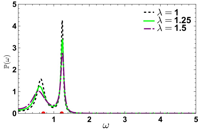
(a) Plot of $\mathbb{P}(\omega)$ when $\lambda=1,1.25,1.5$

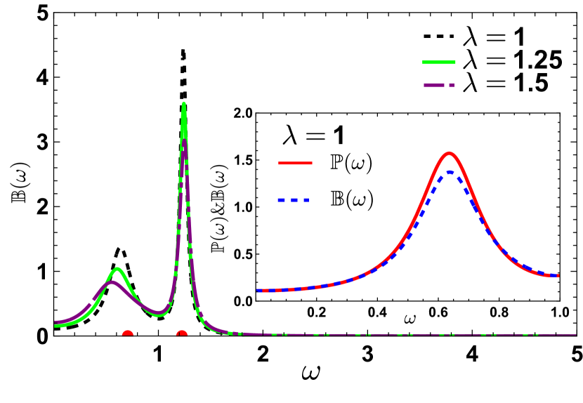
(b) Plot of $\mathbb{B}(\omega)$ when $\lambda=1,1.25,1.5$. The subgraph compares $\mathbb{P}(\omega)$ with $\mathbb{B}(\omega)$ in $\lambda=1$ case.

Figure 1: Plots of $\mathbb{P}(\omega)$ in (a) and $\mathbb{B}(\omega)$ in (b) when $\lambda=1,1.25,1.5$. Here we consider the super Drude dissipation in Eq. (30) for an easy example. We select other parameters of the composite two-mode Brownian oscillator system to be $\Omega_{\mbox{\tiny B}}=1$, $\gamma_{\mbox{\tiny B}}=1.25$ and $V_{11}=V_{22}=1$ and $V_{12}=V_{21}=0.5$. Strength of the couplings are chosen to be $\eta_{1}=0.2$ and $\eta_{2}=0.1$. The red dots on the horizontal axes represent $\omega=0.7071$ and $\omega=1.224$, respectively, which are the square root of eigenvalues of the matrix $\bm{\Omega}\bm{V}$.

In fact we can prove [24] that

$$\lim\limits_{\{c_{\alpha uj}\}\rightarrow\{0\}}\mathbb{P}(\omega)=\sum_{i}\big{[}\delta(\omega-\omega_{i})+\delta(\omega+\omega_{i})\big{]},$$ (31)

where the summation is over all the square root of eigenvalues of the matrix $\bm{\Omega}\bm{V}$. These results show that in the weak coupling limit, only typical closed systems contribute to the quantity that we consider, such as the energy. In other words, the energy of the open system reads

$$E_{\text{weak}}(\beta)=n_{\mbox{\tiny S}}\sum_{i}\frac{\omega_{i}}{2}\coth\frac{\beta\omega_{i}}{2},$$ (32)

which reduces to $\sum_{i}1/2\beta$ in the high-temperature limit $\beta\rightarrow 0$. That is how quantum equipartition reduces to the classical one.

I Summary

To summarize, we derived the generalized quantum equipartition of arbitray quadratic systems and proved the positivity and normalization of their two probability density functions. We also extended another formula for the internal energy of the multi-mode Brownian oscillator system. The generalized formula as well as our analysis shed light on the controversise upon the method. We noticed that our quantum equipartition theorem can be used to obtain the partition function of the system in a much easier way compared to the classical approach [28]. Our results can be viewed as an indispensable generalization of rencent works on quantum equipartition theorem.

As a future prospect, expressing thermodynamic quantities as an infinite series also offers potential advantages for this objective [23]. Work in this direction is in progress. As another point, it seems difficult to discuss the equipartition theorem without the help of fluctuation-disspation theorem or to consider the equipartition theorem over steady states, or even in general nonequilibrium. Discussing the equipartition theorem under other more difficult setups, such as quartic systems, is also challenging. All of them constitute other directions of further development.