Universally Robust Quantum Control

Abstract

We study the robustness of the evolution of a quantum system against small uncontrolled variations in parameters in the Hamiltonian. We show that the fidelity susceptibility, which quantifies the perturbative error to leading order, can be expressed in superoperator form and use this to derive control pulses which are robust to any class of systematic unknown errors. The proposed optimal control protocol is equivalent to searching for a sequence of unitaries that mimics the first-order moments of the Haar distribution, i.e. it constitutes a 1-design. We highlight the power of our results for error resistant single- and two-qubit gates.

Introduction.– Tremendous advances in the ability to manipulate states of light and matter are ushering in the new generation of quantum-enhanced devices. As recently remarked Koch et al. (2022), it is precisely the ability to develop schemes to control a system that endows scientific knowledge with the potential to revolutionise technological landscapes Deutsch (2020); Preskill (2018). However, while exquisite levels of control are now routinely applied in a variety of platforms Larrouy et al. (2020); Lysne et al. (2020); Werninghaus et al. (2021), there will always be systematic errors due to imperfect fabrication and incomplete knowledge of the parameters, either in relation to the model itself or the ambient conditions under which it is operating. Thus, several strategies to explicitly mitigate such errors have been devised, e.g. shortcuts to adiabaticity Guéry-Odelin et al. (2019); Ruschhaupt et al. (2012); Kiely and Ruschhaupt (2014), numerical optimization Koch et al. (2022); Anderson et al. (2015); Coopmans et al. (2022), geometric space curves Dong et al. (2021); Buterakos et al. (2021); Barnes et al. (2022), and dynamical decoupling Lidar (2014).

When these systematic errors are important, typically the control problem is cast in such a way that two, sometimes implicit, assumptions are made regarding the source of the error: (i) that it arises from a weak perturbation, and (ii) that its mathematical structure is exactly known. While the former is a reasonable working condition to assume (if it were not then the fundamental description of the system would need to be adjusted), the latter is arguably less well justified. Indeed, concerted effort is currently invested in identifying the correct physical description of noisy intermediate-scale quantum devices, e.g. determining the most relevant noise sources that they are subject to in order to enhance their efficacy Rudinger et al. (2021). Ultimately there will always be some level of uncertainty in our knowledge of the precise structure of the noise and therefore it is highly desirable to develop a framework that allows to coherently manipulate quantum systems even in the presence of an unknown (even possibly unknowable) source of error.

In this work we develop such a framework which accounts for this uncertainty, termed universally robust control (URC). It provides a straightforward cost function to be minimised to ensure generic robustness in quantum control problems. It can also be easily restricted to specific classes of errors, to account for a limited but useful knowledge of the error type.

Fidelity in the presence of systematic error.–Consider the full system Hamiltonian $H_{\lambda}(t)\!=\!H_{0}(t)+\lambda V$ where $H_{0}(t)$ is the error-free control Hamiltonian, $V$ is the error operator acting with unknown strength, $\lambda$. We assume a pure initial state, $\sigma$, with no $\lambda$ dependence.

The time evolution operator of $H_{\lambda}(t)$ is given by $U_{\lambda}(t,0)$, which leads to a state (which is dependent on $\lambda$) $\rho_{\lambda}\!=\!U_{\lambda}(t_{f},0)\sigma U^{\dagger}_{\lambda}(t_{f},0)$ at the final time $t\!=\!t_{f}$. The fidelity between the perturbed and ideal evolution is $F(\lambda)\!=\!\mbox{Tr}(\rho_{\lambda}\rho_{0})$, which can be expanded for small $\lambda$ as

$$F(\lambda)\approx F(0)+F^{\prime}(0)\lambda+\frac{1}{2}F^{\prime\prime}(0)\lambda^{2}.$$ (1)

By definition $F(0)=1$ and from this follows $F^{\prime}(0)=0$.

The second derivative can be calculated by noting that, for pure states, $\partial_{\lambda}^{2}\rho_{\lambda}\!=\!2\left(\partial_{\lambda}\rho_{\lambda}\right)^{2}+\rho_{\lambda}\left(\partial_{\lambda}^{2}\rho_{\lambda}\right)+\left(\partial_{\lambda}^{2}\rho_{\lambda}\right)\rho_{\lambda}$. Multiplying by $\rho_{0}$ and evaluating the trace at $\lambda\!=\!0$ we get

$$F^{\prime\prime}(0)=-2\>\chi_{S}(\rho_{\lambda}),$$ (2)

where $\chi_{S}(\rho_{\lambda})=\mbox{Tr}\left\{\rho_{0}\left(\partial_{\lambda}\rho_{\lambda}\right)^{2}\big{\lvert}_{\lambda=0}\right\}$ is the fidelity susceptibility Liu et al. (2020), which quantifies how sensitive the evolution is with respect to small perturbations, i.e. $F(\lambda)\!\simeq\!1-\chi_{S}(\rho_{\lambda})\lambda^{2}$. It is clear that $\chi_{S}(\rho_{\lambda})$ is simply the quantum Fisher information (QFI) associated to the family of states $\{\rho_{\lambda}\}$ Sup . The QFI quantifies how much information about $\lambda$ is encoded in the evolution of the state and, therefore, minimizing the QFI at $\lambda=0$ is equivalent to increasing the robustness of a control protocol.

Evaluating explicitly the QFI we find Sup

$$\chi_{S}(\rho_{\lambda})=\frac{t_{f}^{2}}{\hbar^{2}}\left(\Delta\overline{V}_{0}\right)^{2},$$ (3)

where

$$\overline{V}_{0}=\frac{1}{t_{f}}\int_{0}^{t_{f}}ds\>U_{0}^{\dagger}(s,0)VU_{0}(s,0),$$ (4)

is the time average of $V$ in the interaction picture with respect to the unperturbed evolution and the variance is taken with respect to the initial state, $\left(\Delta\overline{V}_{0}\right)^{2}=\mbox{Tr}[\sigma\overline{V}_{0}^{2}]-\mbox{Tr}[\sigma\overline{V}_{0}]^{2}$.

A similar result can be derived for the case of the evolution of unitaries (instead of states). By defining the corresponding fidelity as $F_{U}(\lambda)\!=\!\frac{1}{d^{2}}\left|\mathrm{Tr}\left(U_{0}^{\dagger}U_{\lambda}\right)\right|^{2}$, we obtain that $F_{U}(\lambda)\simeq 1-\chi_{U}(U_{\lambda})\lambda^{2}$ Sup . The susceptibility is

$$\chi_{U}(U_{\lambda})=\frac{t_{f}^{2}}{\hbar^{2}d}||\overline{V}_{0}||^{2},$$ (5)

where $||\cdot||$ is the norm associated with the Hilbert-Schmidt inner product $\left(A|B\right)=\mbox{Tr}(A^{\dagger}B)$ and $d$ is the Hilbert space dimension. Robust control protocols then correspond to finding a $H_{0}(t)$ such that $\rho_{0}\!=\!\rho_{\mathrm{target}}$ or $U_{0}(t_{f},0)=U_{\mathrm{target}}$ while concurrently minimizing $\chi_{S}$ for a known perturbation model $V$ Ball et al. (2021); Koswara et al. (2021); Kosut et al. (2022). We now demonstrate that such robust control can be achieved even without knowledge of $V$.

Universally robust control.–Our construction is based on a superoperator picture where the operator

$$\mathcal{M}_{0}[V]\equiv\overline{V}_{0},$$ (6)

can be seen as the action of a (linear) superoperator $\mathcal{M}_{0}$ acting on $V$ and we assume that $\mbox{Tr}V=0$ . To construct it more explicitly, we go to a doubled Hilbert space. If our original Hilbert space $\mathcal{H}$ is spanned by the orthonormal basis $\{\left|i\right\rangle\}$ where $i=1,\ldots,d$, we take

$$A=\sum\limits_{ij}A_{ij}|i\rangle\langle j|\rightarrow\left|A\right)=\sum\limits_{ij}A_{ij}\left|i\right\rangle\otimes\left|j\right\rangle,$$ (7)

where now the vector $\left|A\right)$ lives in $\mathcal{H}\otimes\mathcal{H}$. Thus, from Eq. (6) we can define

$$M_{0}=\frac{1}{t_{f}}\int_{0}^{t_{f}}ds\left[U_{0}(s,0)\otimes U_{0}(s,0)^{*}\right]^{\dagger}.$$ (8)

such that $\left|\overline{V}_{0}\right)=M_{0}\left|V\right)$. The fidelity susceptibility of Eq. (5) can be expressed in terms of the superoperator $M_{0}$ as

$$||\overline{V}_{0}||^{2}=\left(V\right|M_{0}^{\dagger}M_{0}\left|V\right).$$ (9)

By virtue of Eq. (5) we can increase the robustness of a unitary control protocol irrespective of $V$ by choosing $H_{0}(t)$ to minimize the operator norm of $M_{0}$. This also holds for state control, c.f. Eq. (3), because $\Delta\overline{V}_{0}$ is upper bounded by $||M_{0}||$  Sup .

The trace of any operator $V$ is unitarily invariant. For the identity operator $\mathbb{I}$, $M_{0}\left|\mathbb{I}\right)\!=\!\left|\mathbb{I}\right)$ so the norm of $M_{0}$ cannot be arbitrarily reduced. To sidestep this issue, we restrict to the set of traceless perturbation operators by defining the projector in the doubled Hilbert space $\mathbb{P}_{0}\!=\!\left|\mathbb{I}\right)\left(\mathbb{I}\right|/d$ such that $\mathbb{P}_{0}\left|A\right)\!=\!\mbox{Tr}(A)\left|\mathbb{I}\right)/d$, and redefine the relevant superoperator

$$\tilde{M}_{0}=M_{0}(\mathbb{I}-\mathbb{P}_{0}).$$ (10)

For any operator $V^{\prime}$, this acts as

$$\tilde{M}_{0}\left|V^{\prime}\right)=M_{0}(\mathbb{I}-\mathbb{P}_{0})\left|V^{\prime}\right)=M_{0}\left|V\right)=\left|\overline{V}_{0}\right),$$ (11)

where $V$ is a traceless version of $V^{\prime}$.

The goal of URC is then to minimize the norm of the modified superoperator $\tilde{M}_{0}$, which is related to the previous norm as

$$||\tilde{M}_{0}||^{2}=||M_{0}||^{2}-\mbox{Tr}(M_{0}^{\dagger}M_{0}\mathbb{P}_{0})=||M_{0}||^{2}-1.$$ (12)

This allows us to find choices of $U_{0}$ which yield $\tilde{M}_{0}\!\simeq\!0$, thus achieving $\left|\overline{V}_{0}\right)\simeq 0$ for any $V$.

To understand how a single solution for $U_{0}(t)$ can be made robust to arbitrary perturbations, we note the following connection with unitary designs Gross et al. (2007); Roberts and Yoshida (2017). Discretizing the integral in Eq. (4) into $L\!\gg\!1$ intervals, we find $\overline{V}_{0}\sim\frac{1}{L}\sum\limits_{k=1}^{L}U_{0}^{(k)\dagger}VU_{0}^{(k)}$, which has the form of an average of the operator $V$ conjugated over a discrete set of unitaries, $U_{0}^{(k)}$. If the distribution of such unitaries is uniform according to the Haar measure Collins and Śniady (2006), then it is known that the average

$$\mathbb{E}_{\{U_{0}^{(k)}\}}[U^{\dagger}VU]=\frac{1}{d}\mbox{Tr}(V)$$ (13)

vanishes for all traceless $V$ Collins and Śniady (2006). A less stringent requirement is for the distribution to only match the first-order moment of the uniform distribution, i.e. to be a 1-design. In fact, since $\mathbb{P}_{0}\left|A\right)=\mbox{Tr}(A)\left|\mathbb{I}\right)/d$, we see that the requirement $\tilde{M}_{0}=0$ immediately implies Eq. (13) for any operator, thus making the path traced by the unitary evolution operator $U_{0}(t)$ a 1-design.

Leveraging randomization to increase robustness in quantum processes is routinely done in the context of quantum computing, particularly by tools like dynamical decoupling Zanardi (1999); Lidar (2014), dynamically corrected gates Khodjasteh and Viola (2009); Khodjasteh et al. (2012); Buterakos et al. (2021) and randomized compiling Wallman and Emerson (2016). Our work shows that, for general quantum systems, it is possible to translate this connection into a requirement on a single object, the superoperator $\tilde{M}_{0}$, leading to robustness to any perturbation to first order. As we show in the following, this allows us to set up a quantum optimal control problem to find evolutions that reach a predefined target while at the same time remain robust to arbitrary perturbations.

Optimal control.–We now demonstrate how URC can be naturally leveraged in numerical optimizations. A generic quantum optimal control (QOC) approach considers a series of control parameters, $\{\phi_{k}\}$, which determine the time dependence of $H_{0}(t)$ and aims to maximize the fidelity between a target process $U_{\mathrm{target}}$ and the actual (ideal) evolution operator $U_{0}(t_{f},0)$ by minimizing a cost functional $J_{0}\!=\!1-F_{U}(U_{\mathrm{target}},U_{0}(t_{f},0))$ with respect to $\{\phi_{k}\}$. Additionally, robust QOC usually aims at achieving resilience to perturbations characterized by a known operator $V$. For this task, one can concurrently minimize the fidelity susceptibility given by the control functional $J_{V}\!=\!\frac{1}{d}||\overline{V}_{0}||^{2}$ (see for instance Kosut et al. (2022); Khodjasteh et al. (2012)). Our proposed approach of universally robust QOC instead aims at achieving robustness to an unknown error operator $V$. This can be achieved by instead minimizing the functional $J_{\mathrm{U}}=\frac{1}{d}||\tilde{M}_{0}||^{2}$.

We begin with the simple case of a single qubit with restricted controls with Hamiltonian

$$H_{0}(t)=\Omega\left[\cos\phi(t)\sigma_{x}+\sin\phi(t)\sigma_{y}\right],$$ (14)

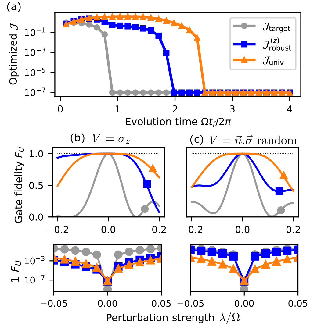
where $\sigma_{\alpha}$ are the Pauli operators, and we consider the control field $\phi(t)$ to be piecewise constant with time steps $\Delta t$ and values $\{\phi_{k}\}$, $k\!=\!1,\ldots,N_{P}$ . The model in Eq. (14) is fully controllable Boozer (2012); Poggi (2019). We set the target transformation to be $U_{\mathrm{target}}\!=\!\exp(-i\sigma_{z}\pi/2)$ and numerically seek the QOC parameters that minimize either only $\mathcal{J}_{\mathrm{target}}\!=\!J_{0}$, $\mathcal{J}_{\mathrm{robust}}\!=\!(J_{0}+wJ_{V=\sigma_{z}})/(1+w)$ or $\mathcal{J}_{\mathrm{URC}}\!=\!(J_{0}+wJ_{\mathrm{U}})/(1+w)$, where $w$ is a non-negative weight which can be changed to improve the resulting balance between the terms. Note that evaluating these functionals requires only computing the error-free evolution given by $H_{0}(t)$, and so no numerical simulations of the perturbed dynamics are required at any stage. In Fig. 1(a) we plot the optimized functional for each case against the evolution time $t_{f}$. The curves display behavior reminiscent of Pareto-fronts Chakrabarti et al. (2008); Caneva et al. (2009), indicative of the fact that optimization always succeeds for sufficiently large $t_{f}$, with the optimization failing when the time becomes too constrained. A minimum control time, $t_{\mathrm{MCT}}$, can be assigned to each process by identifying the minimum value of $t_{f}$ such that the optimization succeeds (which in this case we take as yielding functional values below $10^{-7}$). For target-only and robust control optimizations, we find $t_{MCT}^{\rm T}\!=\!2\pi/\Omega$ and $t_{MCT}^{\rm R}\!=\!4\pi/\Omega$ which are consistent with previous analytical and numerical studies Boozer (2012); Poggi (2019). In contrast, universally robust control demands $t_{MCT}^{\rm U}\!=\!5\pi/\Omega$ (see also Cao et al. (2023)).

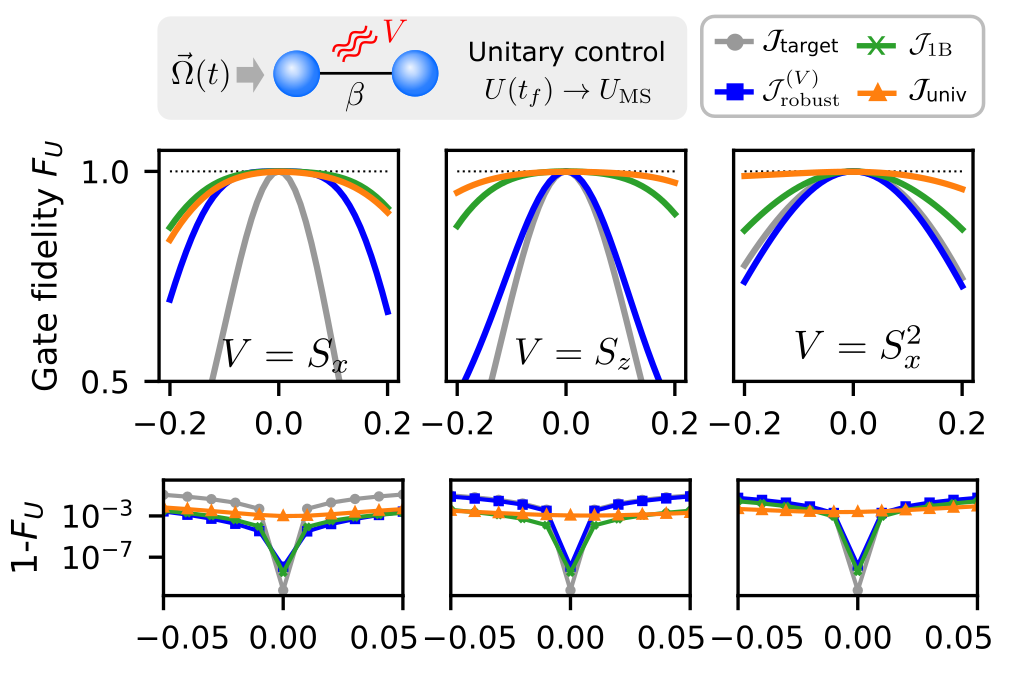
Figure 1: Universal robust control for single-qubit gates. (a) Optimized control functionals as a function of the total evolution time $t_{f}$ for target-only control (gray, circles), target and robustness to a known $V$ (blue, squares) and target and robustness to an unknown $V$ (orange, triangles). (b) and (c) Gate fidelity as a function of perturbation strength $\lambda$ for the cases where $V=\sigma_{z}$ (b) and $V=\vec{n}\cdot\vec{\sigma}$ with $\vec{n}$ a random unit vector (results shown correspond to the average fidelity over 20 realizations). Lower panels shows zoomed-in data of the infidelity $1-F$ in logarithmic scale. We choose a target $U_{\mathrm{target}}=\exp(-i\sigma_{z}\pi/2)$, $N_{P}=40$ control parameters, a balanced functional $w=1$, and an operation time $\Omega t_{f}/(2\pi)=3.5$ for (b) and (c).

To characterize how these longer control waveforms yield robust control processes, we study how well the evolution under the perturbed Hamiltonian $H_{\lambda}(t)=H_{0}(t)+\lambda V$ is able to achieve the target transformation. Fig. 1 shows the cases for (b) $V=\sigma_{z}$ and (c) $V=\vec{n}\cdot\vec{\sigma}$ with $\vec{n}$ a randomly chosen unit vector. The gate fidelity is plotted against the uncertainty parameter $\lambda$ for the three types of optimal controls found. All cases yield high fidelities if $\lambda\!=\!0$, but the target-only optimization results deviate substantially from the ideal value once $\lambda\!\neq\!0$. In (b), we see that the robust control optimization (blue curve) is insensitive to perturbations in $V\!=\!\sigma_{z}$, as it was designed to be. But (c) reveals that the same control is sensitive to generic perturbations. Remarkably, the URC solution (orange curve) is insensitive to first order with respect to perturbations along any direction. This holds true even accounting for the faster minimal control times required for the other protocols Sup .

Generalized robustness.–Building upon the superoperator in Eq. (10) we can generalize this framework to optimize for robustness to any desired subset of operators. This is particularly relevant for systems beyond a single qubit where the nature of the noise or inhomogeneity is partially known instead of being completely arbitrary. Thus, rather than making a control protocol robust to all possible operators $V$, we can instead focus on achieving robustness to a particular set of perturbations, for instance, those generated by local operators. In this case, we are interested in the action of the superoperator, $M_{0}$, only on this reduced set. The advantage of imposing these generalized robustness requirements is that the optimization is less constrained, as effectively less matrix elements are being minimized. Therefore, it is easier to find good solutions even with restricted control time. For example, the total number of operators for $N$ qubits is $4^{N}$ while for the set of local operators is only $3N$.

Consider a quantum system with Hilbert space dimension, $d$, and an orthonormal operator basis $\left\{\Lambda_{j}\right\}$, $j\!=\!0,1,\ldots d^{2}-1$. We introduce a covering of this basis set, $\{C_{k}\}$, such that $\left\{\Lambda_{j}\right\}\!=\!\bigcup_{k=1}^{K}C_{k}$. The projector onto $C_{k}$ is $\mathcal{P}_{k}(A)\!=\!\sum_{\Lambda_{j}\in C_{k}}\mbox{Tr}(\Lambda_{j}^{\dagger}A)\Lambda_{j}$. In the superoperator picture, this is equivalent to defining $\mathbb{P}_{k}\!=\!\sum_{\Lambda_{j}\in C_{k}}\left|\Lambda_{j}\right)\left(\Lambda_{j}\right|$. These superoperators are clearly projectors, as $\mathbb{P}_{k}^{2}\!=\!\mathbb{P}_{k}$ and $\sum_{k=0}^{K}\mathbb{P}_{k}\!=\!\mathbb{I}$. By construction, we take $\Lambda_{0}\!=\!\mathbb{I}/\sqrt{d}$ so that $\mathbb{P}_{0}$ is defined as before. In order to look for controls which are insensitive to any operator within a given subset we seek to minimize the norm of

$$\tilde{M}_{0}=M_{0}\left(1-\sum_{k\in\eta}\mathbb{P}_{k}\right),$$ (15)

where the sum runs over all relevant operator subsets $\eta$ (typically including $\Lambda_{0}$). Note that $\mathbb{P}_{k}$ corresponds to the operators we do not need to be robust to. To illustrate the procedure of imposing generalized robustness requirements into a QOC problem, consider a model of two-qubits with symmetric controls,

$$H_{0}(t)=\Omega_{x}(t)S_{x}+\Omega_{y}(t)S_{y}+\beta S_{z}^{2},$$ (16)

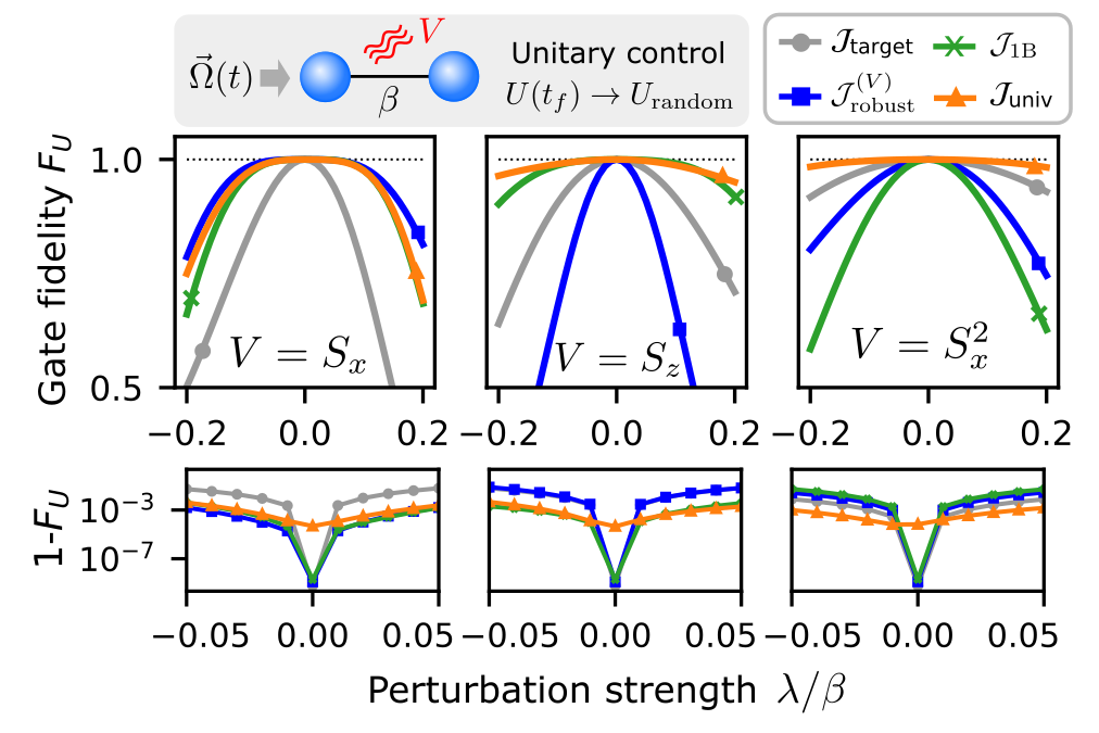
where $S_{\alpha}\!=\!(\sigma_{\alpha}^{(1)}+\sigma_{\alpha}^{(2)})/2$ are collective spin operators and the interaction strength $\beta>0$ is fixed. The perturbation operator, $V$, can be either single-body ($C_{1}$) or two-body ($C_{2}$). We thus have a variety of possible optimization functionals depending on the level of robustness desired. Here we compare three cases: robustness to a single $V\!=\!S_{x}$, robustness to all single-body operators ($V\in C_{1}$) and universal robustness ($V\in C_{1}\cup C_{2}$). We set the target as a randomly-chosen symmetric two-qubit unitary Sup . For this system we find that choosing an unbalanced optimization functional with $w\!=\!0.1$ yields a good compromise between the fidelity at zero perturbation ($\lambda=0$) and the degree of robustness achieved  . In Fig. 2 we show the performance of the optimization using the different functionals introduced thus far, in the presence of various perturbations. As expected, the optimal control procedure is able to find fields which are robust to arbitrary single-body perturbations (green curve), which are not necessarily robust to arbitrary perturbations as the URC (orange curve). On the other hand, the URC solution results in evolutions which are more robust to any type of perturbation, including a two-body one of the form $V=S_{x}^{2}$, when compared to the other methods.

The approach outlined above for designing generalized robustness requirements can be readily carried over to more complex systems. In the Supplementary Material Sup we show additional results that illustrate how this framework can be used to robustly generate entangled states in many-body systems.

Figure 2: Universal robust control for two-qubit gates. Plots show the gate fidelity of the perturbed evolution $H_{0}(t)+\lambda V$, where $H_{0}(t)$ is the control Hamiltonian of Eq. (16). Different curves correspond to different types of optimization procedures: target only (nonrobust, gray circles); target and robustness to a fixed $V_{0}=S_{x}$ (blue squares); target and robustness to all single-body operators (green crosses); target and universal robustness (orange triangles). The lower row shows the infidelity $1-F_{U}$ for each case. Evolution time in all cases is $\beta t_{f}/(2\pi)=5$, and $N_{P}=50$ control parameters are used.

Conclusion.– We have introduced a versatile method, universally robust control (URC), to mitigate the effects of unknown sources of error. By recasting the impact of an arbitrary perturbation to the systems in terms of a single object, here captured by the superoperator in Eq. (8), we showed that since this superoperator has no explicit dependence on the precise operator form of the error, it can be efficiently minimized to provide the necessary, highly robust, control pulses. We demonstrated the effectiveness of our approach for the realization of single- and two-qubit quantum gates, and have shown that it can be generalized to tackle state control problems or to the case of classical fluctuations Kiely (2021). Furthermore, we have demonstrated that the URC formalism can exploit partial information about the source of errors to build arbitrary robustness requirements into the optimal control problem. When combined with powerful numerical optimization techniques, we expect this flexible approach to be able to tackle a broad class of questions in quantum control which are of key importance for the development of quantum technologies. For instance, what is the fundamental trade-off between robustness and experimental constraints (such as bandwidth or evolution time)? how much control resources are required to achieve various levels of robustness in a quantum device? Finally, as our protocol introduces control pulses which dynamically implement $1$-designs, this could be generalized to other $t$-designs which can be readily exploited for quantum computing protocols such as randomized benchmarking Nakata et al. (2021).

Acknowledgments.– The authors acknowledge fruitful discussions with Lorenza Viola. PMP acknowledges support by U.S. National Science Foundation (grant number PHY-2210013) and AFOSR (grant number FA9550-181-1-0064). GDC acknowledges support by the UK EPSRC EP/S02994X/1. SC acknowledges support from the Alexander von Humboldt Foundation. AK and SC are supported by the Science Foundation Ireland Starting Investigator Research Grant “SpeedDemon” No. 18/SIRG/5508.

I Perturbative approximation to the fidelity

I.1 Fidelity susceptibility as the quantum Fisher information

We are interested in calculating the quantum Fisher information (QFI) of the state $\rho_{\lambda}$ with respect to the parameter $\lambda$. Formally, the QFI is defined as $F_{Q}[\rho_{\lambda}]=(\Delta L)^{2}$, which is the variance ($(\Delta x)^{2}=\langle x^{2}\rangle-\langle x\rangle^{2}$) of the symmetric logarithmic derivative $L$ defined implicitly as $\frac{\partial\rho_{\lambda}}{\partial\lambda}=\left(\rho_{\lambda}L+L\rho_{\lambda}\right)/2$ Liu et al. (2020). Note that for pure states we have that

$$\frac{\partial\rho_{\lambda}}{\partial\lambda} = \frac{\partial\rho_{\lambda}^{2}}{\partial\lambda}$$ (S1)

$$= \rho_{\lambda}\frac{\partial\rho_{\lambda}}{\partial\lambda}+\frac{\partial\rho_{\lambda}}{\partial\lambda}\rho_{\lambda}.$$ (S2)

Clearly then for this case, $L=2\frac{\partial\rho_{\lambda}}{\partial\lambda}$. The mean is given by

$$\langle L\rangle = 2\mbox{Tr}\left(\rho_{\lambda}\frac{\partial\rho_{\lambda}}{\partial\lambda}\right)$$ (S3)

$$= \mbox{Tr}\left(\frac{\partial\rho_{\lambda}^{2}}{\partial\lambda}\right)$$ (S4)

$$= \frac{\partial}{\partial\lambda}\mbox{Tr}\rho_{\lambda}^{2}$$ (S5)

$$= 0.$$ (S6)

Therefore the QFI can be compactly written as

$$F_{Q}[\rho_{\lambda}]=4\mbox{Tr}\left[\rho_{\lambda}\left(\frac{\partial\rho_{\lambda}}{\partial\lambda}\right)^{2}\right].$$ (S7)

I.2 Explicit expression for fidelity susceptibility

The derivative of the state can then be expressed as

$$\frac{\partial\rho_{\lambda}}{\partial\lambda}=\frac{\partial U_{\lambda}}{\partial\lambda}\sigma U_{\lambda}^{\dagger}+U_{\lambda}\sigma\frac{\partial U^{\dagger}_{\lambda}}{\partial\lambda}.$$ (S8)

We then use the derivative of the unitary time evolution operator as

$$\frac{dU_{\lambda}(t_{f},0)}{d\lambda}=-\frac{i}{\hbar}\int_{0}^{t_{f}}dsU_{\lambda}(t_{f},s)VU_{\lambda}(s,0).$$ (S9)

Inserting in this relation gives us

$$\frac{\partial\rho_{\lambda}}{\partial\lambda} = -\frac{i}{\hbar}\int_{0}^{t_{f}}ds\left[U_{\lambda}(t_{f},s)VU_{\lambda}(s,0)\sigma U_{\lambda}^{\dagger}(t_{f},0)-U_{\lambda}(t_{f},0)\sigma U^{\dagger}_{\lambda}(s,0)VU^{\dagger}_{\lambda}(t_{f},s)\right]$$ (S10)

$$= -\frac{i}{\hbar}\int_{0}^{t_{f}}ds\left[U_{\lambda}(t_{f},s)VU^{\dagger}_{\lambda}(t_{f},s)U_{\lambda}(t_{f},0)\sigma U_{\lambda}^{\dagger}(t_{f},0)-U_{\lambda}(t_{f},0)\sigma U^{\dagger}_{\lambda}(t_{f},0)U_{\lambda}(t_{f},s)VU^{\dagger}_{\lambda}(t_{f},s)\right]$$ (S11)

$$= -\frac{i}{\hbar}\int_{0}^{t_{f}}ds\left[U_{\lambda}(t_{f},s)VU^{\dagger}_{\lambda}(t_{f},s)\rho_{\lambda}-\rho_{\lambda}U_{\lambda}(t_{f},s)VU^{\dagger}_{\lambda}(t_{f},s)\right]$$ (S12)

$$= -i\left[G_{\lambda},\rho_{\lambda}\right],$$ (S13)

where $G_{\lambda}=\frac{1}{\hbar}\int_{0}^{t_{f}}dsU_{\lambda}(t_{f},s)VU^{\dagger}_{\lambda}(t_{f},s)$. The QFI is then

$$F_{Q}[\rho_{\lambda}] = -4\,\mbox{Tr}\left\{\rho_{\lambda}\left[G_{\lambda},\rho_{\lambda}\right]^{2}\right\}$$ (S14)

$$= -4\,\mbox{Tr}\left\{\rho_{\lambda}\left(G_{\lambda}\rho_{\lambda}G_{\lambda}\rho_{\lambda}-G_{\lambda}\rho_{\lambda}^{2}G_{\lambda}-\rho_{\lambda}G_{\lambda}^{2}\rho_{\lambda}+\rho_{\lambda}G_{\lambda}\rho_{\lambda}G_{\lambda}\right)\right\}$$ (S15)

$$= 4\left(\langle G^{2}_{\lambda}\rangle-\langle G_{\lambda}\rangle^{2}\right)$$ (S16)

$$= 4\left(\Delta G_{\lambda}\right)^{2},$$ (S17)

where these steps hold true for pure states. This can be further simplified by noting that

$$\langle G_{\lambda}\rangle = \mbox{Tr}\left\{G_{\lambda}\rho_{\lambda}\right\}$$ (S18)

$$= \mbox{Tr}\left\{\frac{1}{\hbar}\int_{0}^{t_{f}}dsU_{\lambda}(t_{f},s)VU^{\dagger}_{\lambda}(t_{f},s)U_{\lambda}(t_{f},0)\sigma U^{\dagger}_{\lambda}(t_{f},0)\right\}$$ (S19)

$$= \mbox{Tr}\left\{\frac{1}{\hbar}\int_{0}^{t_{f}}dsU^{\dagger}_{\lambda}(s,0)VU_{\lambda}(s,0)\sigma\right\}$$ (S20)

$$= t_{f}\langle\overline{V}_{\lambda}\rangle_{i}/\hbar,$$ (S21)

where the average $\langle\cdot\rangle_{i}$ is taken over the initial state $\sigma$ and we have defined $\overline{V}_{\lambda}=\frac{1}{t_{f}}\int_{0}^{t_{f}}dsU^{\dagger}_{\lambda}(s,0)VU_{\lambda}(s,0)$ which is the time-averaged version of the operator $V$ in the interaction picture. Similarly, the other term is given by

$$\langle G^{2}_{\lambda}\rangle = \mbox{Tr}\left\{G^{2}_{\lambda}\rho_{\lambda}\right\}$$ (S22)

$$= \mbox{Tr}\left\{G^{2}_{\lambda}U_{\lambda}(t_{f},0)\sigma U^{\dagger}_{\lambda}(t_{f},0)\right\}$$ (S23)

$$= \mbox{Tr}\left\{U^{\dagger}_{\lambda}(t_{f},0)G^{2}_{\lambda}U_{\lambda}(t_{f},0)\sigma\right\}$$ (S24)

$$= \mbox{Tr}\left\{\left[U^{\dagger}_{\lambda}(t_{f},0)G_{\lambda}U_{\lambda}(t_{f},0)\right]^{2}\sigma\right\}$$ (S25)

$$= t_{f}^{2}\langle\overline{V}_{\lambda}^{2}\rangle_{i}/\hbar^{2}.$$ (S26)

Putting this all together now, we have that the QFI can be expressed as a variance of the operator $\overline{V}_{\lambda}$ over the initial $\lambda$-independent state $\sigma$,

$$F_{Q}[\rho_{\lambda}] = \frac{4t_{f}^{2}}{\hbar}\left(\Delta\overline{V}_{\lambda}\right)^{2}.$$ (S27)

I.3 Fidelity susceptibility for unitaries

The relevant fidelity is $F_{U}(\lambda)=\frac{1}{d^{2}}\left|\mbox{Tr}\left(U_{0}^{\dagger}U_{\lambda}\right)\right|^{2}$ Poggi (2019) which we will expand in powers of $\lambda$. Again we make use of Eq. (S9) and start by noting that for any complex scalar $z$, $\frac{d}{dx}(|z|^{2})=2\mathrm{Re}(z^{*}\frac{dz}{dx})$. Therefore

$$\frac{dF_{U}}{d\lambda} =\frac{2}{d^{2}}\mathrm{Re}\left[\mbox{Tr}(U_{\lambda}^{\dagger}U_{0})\mbox{Tr}\left(U_{0}^{\dagger}\frac{dU_{\lambda}}{d\lambda}\right)\right]$$ (S28)

$$=\frac{2}{d^{2}\hbar}\mathrm{Im}\left\{\mbox{Tr}(U_{\lambda}^{\dagger}U_{0})\int_{0}^{t_{f}}ds\>\mbox{Tr}\left[U_{0}^{\dagger}U_{\lambda}(t_{f},s)VU_{\lambda}(s,0)\right]\right\}.$$ (S29)

Evaluating the first derivative at $\lambda=0$ yields

$$\left.\frac{dF_{U}}{d\lambda}\right|_{\lambda=0}=\frac{2}{d\hbar}\mathrm{Im}\left\{\int_{0}^{t_{f}}ds\>\mbox{Tr}\left[U_{0}^{\dagger}(s,0)VU_{0}(s,0)\right]\right\}=\frac{2}{d\hbar}\mathrm{Im}\left[\mbox{Tr}(V)t_{f}\right]=0.$$ (S30)

The second derivative reads

$$\frac{d^{2}F_{U}}{d\lambda^{2}} =\frac{2}{d^{2}\hbar}\mathrm{Im}\left\{\mbox{Tr}\left[\frac{dU_{\lambda}^{\dagger}}{d\lambda}U_{0}\right]\int_{0}^{t_{f}}ds\>\mbox{Tr}\left[U_{0}^{\dagger}U_{\lambda}(t_{f},s)VU_{\lambda}(s,0)\right]\right.+$$

$$\left.\mbox{Tr}(U_{\lambda}^{\dagger}U_{0})\int_{0}^{t_{f}}ds\>\mbox{Tr}\left[U_{0}^{\dagger}\frac{dU_{\lambda}(t_{f},s)}{d\lambda}VU_{\lambda}(s,0)+U_{0}^{\dagger}U_{\lambda}(t_{f},s)V\frac{dU_{\lambda}(s,0)}{d\lambda}\right]\right\}$$ (S31)

$$=\frac{2}{d^{2}\hbar^{2}}\left|\int_{0}^{t_{f}}ds\>\mbox{Tr}\left[U_{0}^{\dagger}U_{\lambda}(t_{f},s)VU_{\lambda}(s,0)\right]\right|^{2}+$$

$$-\frac{2}{d^{2}\hbar^{2}}\mathrm{Im}\left\{i\mbox{Tr}(U_{\lambda}^{\dagger}U_{0})\int_{0}^{t_{f}}ds\>\mbox{Tr}\left[\int_{s}^{t_{f}}dx\>U_{0}^{\dagger}U_{\lambda}(t_{f},x)VU_{\lambda}(x,s)VU_{\lambda}(s,0)+\int_{0}^{s}dx\>U_{0}^{\dagger}U_{\lambda}(t_{f},s)VU_{\lambda}(s,x)VU_{\lambda}(x,0)\right]\right\}.$$ (S32)

When evaluating it at $\lambda=0$, the first term depends on $\mbox{Tr}(V)$ as before, which vanishes. For the second term, we use the cycle property of the trace to find that

$$\left.\frac{d^{2}F_{U}}{d\lambda^{2}}\right|_{\lambda=0} =-\frac{2}{\hbar^{2}d}\mathrm{Im}\left[i\int_{0}^{t_{f}}ds\>\left\{\int_{s}^{t_{f}}dx\>\mbox{Tr}[V(x)V(s)]+\int_{0}^{s}dx\>\mbox{Tr}[V(s)V(x)]\right\}\right]$$ (S33)

$$=-\frac{2}{\hbar^{2}d}\mathrm{Im}\left[i\>\mbox{Tr}\left(\int_{0}^{t_{f}}ds\>V(s)\int_{0}^{t_{f}}dx\>V(x)\right)\right]=-\frac{2t_{f}^{2}}{\hbar^{2}d}\mbox{Tr}\left(\overline{V_{0}}^{2}\right).$$ (S34)

This is exactly the quoted result in Eq.(5).

II Robust state control

Coming back to the original state control problem, we now show how the different universal robustness constraints can be imposed in that case too. Recall the expression of the fidelity susceptibility (or quantum Fisher information) associated with the perturbation-dependent trajectories $\rho_{\lambda}(t)$, Eq. (3). The relevant variance can be written (for a pure initial state) as

$$\left(\Delta\overline{V}_{0}\right)^{2} = \mbox{Tr}[\overline{V}_{0}^{2}\sigma]-\mbox{Tr}[\overline{V}_{0}\sigma\overline{V}_{0}\sigma]$$ (S35)

$$= \left(\overline{V}_{0}\right|\mathbb{I}\otimes\sigma^{*}\left|\overline{V}_{0}\right)-\left(\overline{V}_{0}\right|\sigma\otimes\sigma^{*}\left|\overline{V_{0}}\right)$$ (S36)

$$= \left(V\right|M_{0}^{\dagger}\mathbb{P}_{\sigma}M_{0}\left|V\right),$$ (S37)

where we have defined $\mathbb{P}_{\sigma}=(\mathbb{I}-\sigma)\otimes\sigma^{*}$. This is clearly a projector since

$$\mathbb{P}_{\sigma}^{2} = (\mathbb{I}-\sigma)^{2}\otimes(\sigma^{*})^{2}$$ (S38)

$$= (\mathbb{I}-\sigma-\sigma+\sigma)\otimes\sigma^{*}$$ (S39)

$$= \mathbb{P}_{\sigma}.$$ (S40)

We will now simplify this projector further. Its eigenvectors $\left|\chi_{n}\right)$ with eigenvalue one, must satisfy $\mathbb{P}_{\sigma}\left|\chi_{n}\right)\rightarrow(\mathbb{I}-\sigma)\chi_{n}\sigma=\chi_{n}$. For pure states this simplifies to

$$\left[\chi_{n}-\mbox{Tr}(\sigma\chi_{n})\right]\sigma=\chi_{n}.$$ (S41)

Multiplying on the right by $\sigma$ we can see that the condition reduces to $\left(\sigma|\chi\right)=0$. The projection operator can be written as

$$\mathbb{P}_{\sigma}=\sum_{n}\left|\chi_{n}\right)\left(\chi_{n}\right|,$$ (S42)

where the operators $\chi_{n}$ form an orthogonal basis and which all fulfil $\left(\sigma|\chi_{n}\right)=0$. Written simpler $\mathbb{P}_{\sigma}=\mathbb{I}-\left|\sigma\right)\left(\sigma\right|$, the latter expression leads to

$$\left(\Delta\overline{V}_{0}\right)^{2}=\left\lVert\overline{V}_{0}\right\rVert^{2}-\left|\left(\sigma|\overline{V}_{0}\right)\right|^{2}.$$ (S43)

Note also that by the Cauchy–Schwarz inequality $\left(\Delta\overline{V}_{0}\right)^{2}=\left\lVert\mathbb{P}_{\sigma}M_{0}\left|V\right)\right\rVert^{2}\leq\left\lVert M_{0}\left|V\right)\right\rVert^{2}=\left\lVert\overline{V}_{0}\right\rVert^{2}$. This connects to the case of quantum gates since the last term is state independent, c.f. Eq. (5).

To summarise then, we have

$$\left(\Delta\overline{V}_{0}\right)^{2}=\left(V\right|(M_{0}^{\sigma})^{\dagger}M_{0}^{\sigma}\left|V\right).$$ (S44)

which has the same form as Eq. (9), but introduces the initial-state-dependent superoperator $M_{0}^{\sigma}=\mathbb{P}_{\sigma}M_{0}$. Note that this does not suffer the same difficulty as before since $M^{\sigma}_{0}\left|\mathbb{I}\right)=\mathbb{P}_{\sigma}M_{0}\left|\mathbb{I}\right)=\mathbb{P}_{\sigma}\left|\mathbb{I}\right)=0$.

III Analytical expression of the URC functional gradient

In the following, we will derive a closed form approximation to the gradient of the URC cost functional $J_{\mathrm{U}}$, which could be then used in a variety of gradient based optimization algorithms.

III.1 Gradient of unitary evolution operator

Let us assume the ideal Hamiltonian to be split as a drift and a time-dependent control part: $H(t)=H_{\rm d}+H_{\rm con}(t)$. The time evolution operator under this Hamiltonian is formally $U(t,0)=\mathcal{T}\exp\left[-\frac{i}{\hbar}\int_{0}^{t}H(s)ds\right]$, where $\mathcal{T}$ is the time ordering operator. We assume that the time dependence is piecewise constant, i.e., on the interval $[t_{j},t_{j+1}]$ we have $H_{\rm con}(t)=\phi_{j}W$. The time evolution operator can then be expressed exactly as

$$U(t,0) = \prod_{j}\exp\left[-\frac{i}{\hbar}(H_{\rm d}+\phi_{j}W)\Delta t\right]$$ (S45)

$$= \prod_{j}U_{j},$$ (S46)

where $U_{j}$ is the time evolution operator over constant intervals $\Delta t=t_{j+1}-t_{j}$. We can define the control vector as $\vec{\phi}=(\phi_{1},\phi_{2},\ldots,\phi_{N_{P}})^{T}$. The $k^{\rm th}$ element of the gradient of the time evolution operator with respect to this control vector can be expressed as

$$\{\nabla_{\vec{\phi}}U(t,0)\}_{k} = \prod_{j=k+1}^{N_{P}}U_{j}\left(\partial_{\phi_{k}}U_{k}\right)\prod_{j=1}^{k-1}U_{j}$$ (S47)

$$\approx \prod_{j=k+1}^{N_{P}}U_{j}\left(-\frac{i}{\hbar}\Delta tWU_{k}\right)\prod_{j=1}^{k-1}U_{j},$$ (S48)

where in the second step we have assumed short time intervals $\Delta t$. The gradient over any interval $[t_{a},t_{b}]$ on our mesh can be expressed as

$$\{\nabla_{\vec{\phi}}U(t_{b},t_{a})\}_{k}\approx\begin{cases}0&t_{k}\notin[t_{a},t_{b}]\\ \prod_{j=k+1}^{b}U_{j}\left(-\frac{i}{\hbar}\Delta tWU_{k}\right)\prod_{j=a}^{k-1}U_{j}&\rm{Otherwise}\end{cases}.$$ (S49)

III.2 Gradient of the cost functional $J_{\mathrm{U}}$

We now want to find the gradient of the norm (we assume the Frobenius norm for concreteness) of the superoperator. The norm squared can be first simplified as

$$dJ_{\mathrm{U}} = ||M_{0}||^{2}-1$$ (S50)

$$= \left\lVert\frac{1}{t_{f}}\int\limits_{0}^{t_{f}}dsU(s,0)\otimes U(s,0)^{*}\right\rVert^{2}-1$$ (S51)

$$= \frac{1}{t_{f}^{2}}\mbox{Tr}\left\{\int\limits_{0}^{t_{f}}ds_{2}U(s_{2},0)\otimes U(s_{2},0)^{*}\int\limits_{0}^{t_{f}}ds_{1}\left[U(s_{1},0)\otimes U(s_{1},0)^{*}\right]^{\dagger}\right\}-1$$ (S52)

$$= \frac{1}{t_{f}^{2}}\int\limits_{0}^{t_{f}}ds_{1}\int\limits_{0}^{t_{f}}ds_{2}\mbox{Tr}\left[U(s_{2},0)U^{\dagger}(s_{1},0)\otimes U(s_{2},0)^{*}U(s_{1},0)^{T}\right]-1$$ (S53)

$$= \frac{1}{t_{f}^{2}}\int\limits_{0}^{t_{f}}ds_{1}\int\limits_{0}^{t_{f}}ds_{2}\mbox{Tr}\left[U(s_{2},s_{1})\otimes U(s_{2},s_{1})^{*}\right]-1$$ (S54)

$$= \frac{1}{t_{f}^{2}}\int\limits_{0}^{t_{f}}ds_{1}\int\limits_{0}^{t_{f}}ds_{2}\mbox{Tr}\left[U(s_{2},s_{1})\right]\mbox{Tr}\left[U(s_{2},s_{1})^{*}\right]-1$$ (S55)

$$= \frac{1}{t_{f}^{2}}\int\limits_{0}^{t_{f}}ds_{1}\int\limits_{0}^{t_{f}}ds_{2}\left|\mbox{Tr}\left[U(s_{2},s_{1})\right]\right|^{2}-1.$$ (S56)

Note that by the Cauchy-Schwartz inequality and the fact that the time evolution operator is unitary we get that $J_{\rm U}\leq d-1/d$.

The $k^{\rm th}$ component of the gradient is then

$$\partial_{\phi_{k}}J_{\mathrm{U}} = \frac{1}{dt_{f}^{2}}\int\limits_{0}^{t_{f}}ds_{1}\int\limits_{0}^{t_{f}}ds_{2}\partial_{\phi_{k}}\left|\mbox{Tr}\left[U(s_{2},s_{1})\right]\right|^{2}$$ (S57)

$$= \frac{2}{dt_{f}^{2}}\int\limits_{0}^{t_{f}}ds_{1}\int\limits_{0}^{t_{f}}ds_{2}\mathrm{Re}\left\{\mbox{Tr}\left[U(s_{2},s_{1})\right]\partial_{\phi_{k}}\mbox{Tr}\left[U(s_{2},s_{1})\right]^{*}\right\}$$ (S58)

$$= \frac{2}{dt_{f}^{2}}\int\limits_{0}^{t_{f}}ds_{1}\int\limits_{0}^{t_{f}}ds_{2}\mathrm{Re}\left\{\mbox{Tr}\left[U(s_{2},s_{1})\right]\mbox{Tr}\left[\partial_{\phi_{k}}U(s_{2},s_{1})\right]^{*}\right\}.$$ (S59)

This could be computed numerically using the following steps. First compute all $U_{j}$ for a given vector $\vec{\phi}$. Then, the derivative can be approximated as

$$\partial_{\phi_{k}}J_{\mathrm{U}}\approx\frac{2(\Delta t)^{2}}{dt_{f}^{2}}\sum_{n,m=1}^{N_{P}-1}\mathrm{Re}\left\{\mbox{Tr}\left[U(t_{m},t_{n})\right]\mbox{Tr}\left[\partial_{\phi_{k}}U(t_{m},t_{n})\right]^{*}\right\}$$ (S60)

where $U(t_{m},t_{n})=U_{m}\ldots U_{n}$ and each component of the gradient of $U$ is approximated by Eq. (S49).

In order to reduce the computation time in calculating $U_{j}$, one could use the Baker-Campbell-Hausdorff approximation as

$$U_{j}\approx\exp\left[-\frac{i}{\hbar}(\Delta t)H_{\rm d}\right]\exp\left[-\frac{i}{\hbar}(\Delta t)\phi_{j}W\right]\exp\left[\frac{1}{2\hbar^{2}}(\Delta t)^{2}\phi_{j}[H_{\rm d},W]\right],$$ (S61)

provided that $\Delta t$ was sufficiently small. Precomputing the spectrum of $H_{\rm d}$, $W$ and $[H_{\rm d},W]$ would make the repeated matrix exponentiation much faster.

IV Extension to classical fluctuations

Consider now the Hamiltonian $H(t)=H_{0}(t)+\lambda\xi(t)V$. The noise averaged state fidelity is given to second order in $\lambda$ as

$$\langle F_{\xi}\rangle\approx 1-\frac{\lambda^{2}}{\hbar^{2}}\int_{0}^{\tau}dt\int_{0}^{\tau}dsC(t,s)\left[\langle V_{I}(t)V_{I}(s)\rangle-\langle V_{I}(t)\rangle\langle V_{I}(s)\rangle\right],$$ (S62)

where $V_{I}(t)=U_{0}^{\dagger}(t,0)VU_{0}(t,0)$ is the noise operator $V$ in the interaction picture and the noise $\xi(t)$ has zero mean and correlation function $C(t,s)=\langle\xi(t)\xi(s)\rangle$. We can define a superoperator $N_{t}=\left[U_{0}(t,0)\otimes U^{*}_{0}(t,0)\right]^{\dagger}$, such that $\left|V_{I}(t)\right)=N_{t}\left|V\right)$. The first term in the operator Hilbert space can then be expressed as

$$\langle V_{I}(t)V_{I}(s)\rangle=\left(V\right|N_{t}^{\dagger}\mathbb{I}\otimes\sigma^{*}N_{s}\left|V\right).$$ (S63)

Similarly the product of averages becomes

$$\langle V_{I}(t)\rangle\langle V_{I}(s)\rangle = \mbox{Tr}[V_{I}(t)\sigma V_{I}(s)\sigma]$$ (S64)

$$= \left(V\right|N_{t}^{\dagger}\sigma\otimes\sigma^{*}N_{s}\left|V\right).$$ (S65)

All together then, this can be written as

$$\langle F_{\xi}\rangle\approx 1-\frac{\lambda^{2}}{\hbar^{2}}\int_{0}^{\tau}dt\int_{0}^{\tau}ds\,C(t,s)\left(V\right|N_{t}^{\dagger}\mathbb{P}_{\sigma}N_{s}\left|V\right).$$ (S66)

Thus, to minimise the impact of the noise regardless of the operator $V$, one must minimise the operator

$$\int_{0}^{\tau}dt\int_{0}^{\tau}ds\,C(t,s)N_{t}^{\dagger}\mathbb{P}_{\sigma}N_{s}.$$ (S67)

V Additional numerical results

In this section, we present additional numerical results. These include further applications of the URC framework and more detailed descriptions of the problems analyzed in the main text.

V.1 Generation of many-body entangled states

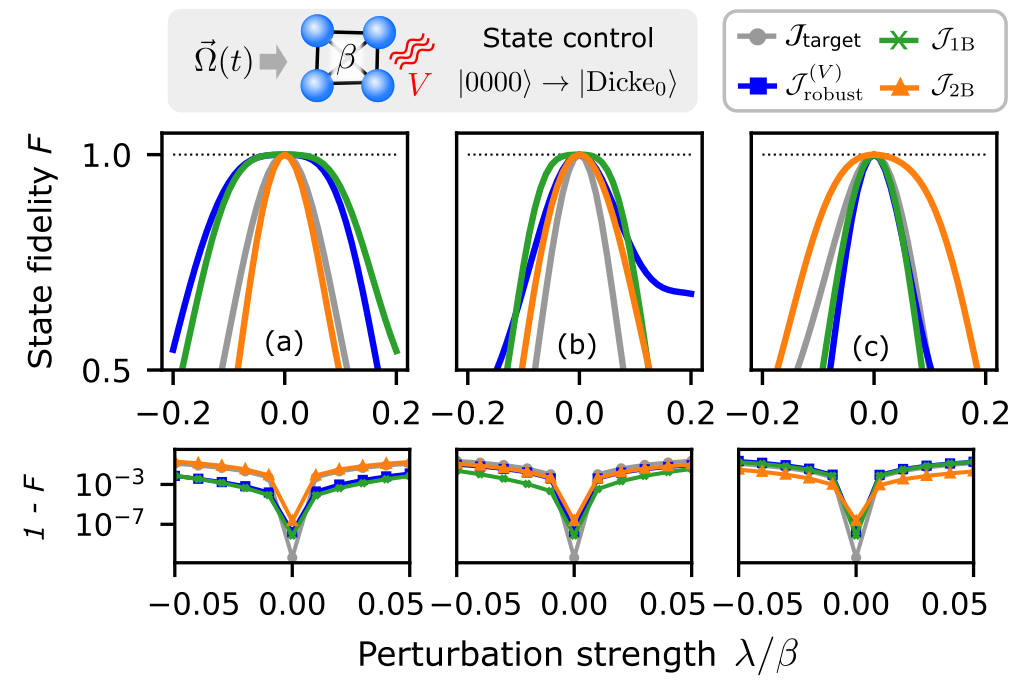
Figure S1: Universal robust control for four-qubit state-control problem. Top panels show the state fidelity $F$, bottom panels show a zoomed-in view of the infidelity $1-F$. In all cases data is plotted against the perturbation strength $\lambda$ for the evolution $H_{0}(t)+\lambda V_{x}$ where (a) $V_{a}=V=S_{x}$, (b) $V_{b}=S_{z}$, (c) $V_{c}=S_{x}^{2}$. The four curves correspond to the four optimization functionals described in the text, c.f. Eqns. (S68)-(S70).

Eq. (S44) allows us to carry over the optimal control procedure discussed in the main text for unitary control to the problem of robust state control. The only adaptation needed is to replace $M_{0}$ with $M_{0}^{\sigma}$. We illustrate this procedure by analyzing the problem of generating entangled states in a system of $N=4$ qubits with global controls and all-to-all interactions. We consider a Hamiltonian having the exact same form as (16) where now $S=N/2$ is the total angular momentum associated with the symmetric subspace of the $N$ particles. We point out that this problem is fully controllable for any $N$ Merkel et al. (2008). We consider the problem of driving the system from the state $\left|0000\right\rangle$ to the Dicke-0 state, i.e. the eigenstate of $S_{z}$ composed of a symmetric superposition of states with equal number of qubits in 0 and in 1. Because this is a four-body system, there many possible choices of robustness setups that could be pursued. Here we demonstrate the flexibility of our approach by showing results corresponding to robustness to either all single-body or all two-body operators in Fig. S1. In all plots we show four curves, corresponding to four functionals being optimized. These are

$$\mathcal{J}_{\mathrm{target}} =J_{0}$$ (S68)

$$\mathcal{J}_{\mathrm{robust}}^{(V)} =(J_{0}+wJ_{V})/(1+w),\ \text{where}\ V=S_{x}$$ (S69)

$$\mathcal{J}_{\eta} =(J_{0}+wJ_{\mathrm{U}}^{(\eta)})/(1+w),\ \text{where}\ \eta=\text{1B},\ \text{2B}$$ (S70)

The URC functionals $J_{\mathrm{U}}^{(\eta)}=||\tilde{M_{0}}^{(\eta)}||^{2}/d$ differ in the case of seeking robustness to just 1-body operators (1B) or just 2-body operators (2B):

$$M_{0}^{\text{1B}} =M_{0}\left(1-\sum\limits_{k\neq 1}\mathbb{P}_{k}\right),$$ (S71)

$$M_{0}^{\text{2B}} =M_{0}\left(1-\sum\limits_{k\neq 2}\mathbb{P}_{k}\right),$$ (S72)

where $\mathbb{P}$ denotes the projector onto $k-$body operators. Fig. S1 shows the fidelity as a function of perturbation strength $\lambda$ for every solution in the presence of three different perturbations; in other words we calculate the state fidelity achieved by the dynamics $H_{0}(t)+\lambda V_{x}$ where $x=a,b,c$ labels the different panels in the figure: (a) $V_{a}=V=S_{x}$, (b) $V_{b}=S_{z}$, (c) $V_{c}=S_{x}^{2}$ (these are the same choices used for the two-qubit case of Fig. 2). The results show that every optimization delivers the expected results: the usual robust control is only insensitive to the predefined choice of $V$, but remains sensitive to other perturbations. On the other hand, the URC waveforms designed to be insensitive to all single-body perturbations (1B) shows robustness in both cases (a) and (b). Likewise, the URC waveforms 2B are only robust to the case where the noise is on a two-body operator (c).

V.2 Comparison of timescales

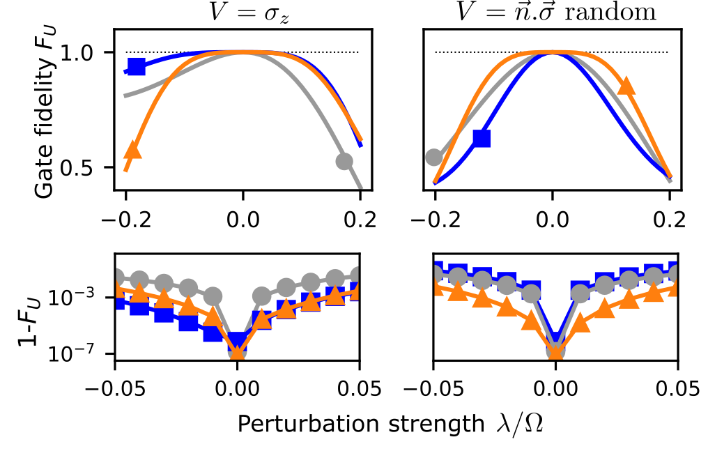
Figure S2: Performance of Universal Robust Control when compared to other approaches and restricting the evolution time. The parameters are as in Fig. 1, with the exception that for URC (orange triangles) $\Omega t_{f}^{\rm U}/(2\pi)=3.5$; for the standard robust control $\Omega t_{f}^{\rm R}/(2\pi)=2.1$, for the nonrobust control $\Omega t_{f}^{\rm T}/(2\pi)=1.1$.

In Fig. 1, we demonstrated how the URC waveforms leads to enhanced robustness with respect to perturbations when compared outperform the other controls analyzed. These correspond to the output of optimizing either $\mathcal{J}_{\text{target}}$ or $J_{\text{robust}}$. The evolutions studied in Fig. 1 correspond to all waveforms of the same duration $\Omega t_{f}/(2\pi)=3.5\pi$. A fair critique of this analysis is that nonrobust or standard robust waveforms can be achieved with shorter operation times. Therefore we compare in Fig. S2 the performance of waveforms of different durations, which now scale with their respective minimal control time (indicated in the main text). While not as striking, it is still clearly from these results that the URC method still provides additional stability overall, despite needing extra time to do so.

V.3 Other target states

Figure S3: Universal robust control for two-qubit gates. Plots show the gate fidelity of the perturbed evolution $H_{0}(t)+\lambda V$, where $H_{0}(t)$ is the control Hamiltonian of Eq. (16). Different curves correspond to different types of optimization procedures: target only (nonrobust, gray circles); target and robustness to a fixed $V_{0}=S_{x}$ (blue squares); target and robustness to all single-body operators (green crosses); target and universal robustness (orange triangles). Lower row shows the infidelity $1-F$ for each case.

In the analysis of two-qubit unitary control, we set as a target transformation a single, randomly-chosen, two-qubit symmetric gate. When written in the symmetric basis $\{\left|00\right\rangle,(\left|01\right\rangle+\left|10\right\rangle)/\sqrt{2},\left|11\right\rangle\}$, such gate has the form

$$U_{\text{random}}=\left(\begin{array}[]{c c c}0.51762131+0.11456864i&-0.5988566-0.16086483i&-0.57589678+0.05271048i\\ -0.22709248+0.22335233i&0.30541094+0.57529237i&-0.6568961-0.20686492i\\ -0.75950102+0.20160146i&-0.40091574-0.17470746i&-0.13888378+0.41469292i\end{array}\right).$$ (S73)

A more physically-inspired choice could be the XX Mølmer-Sørensen (MS) gate,

$$U_{\text{MS}}=\exp\left[-i\frac{\pi}{2}\left(S_{x}^{2}-\frac{1}{2}S_{x}\right)\right].$$ (S74)

In Fig. S3 we show results which are completely analogous to Fig. 2, but now setting as a target the MS gate. As is evident from the data, the URC framework works irrespectively of the choice of target gate.

V.4 Further details on the numerical optimization

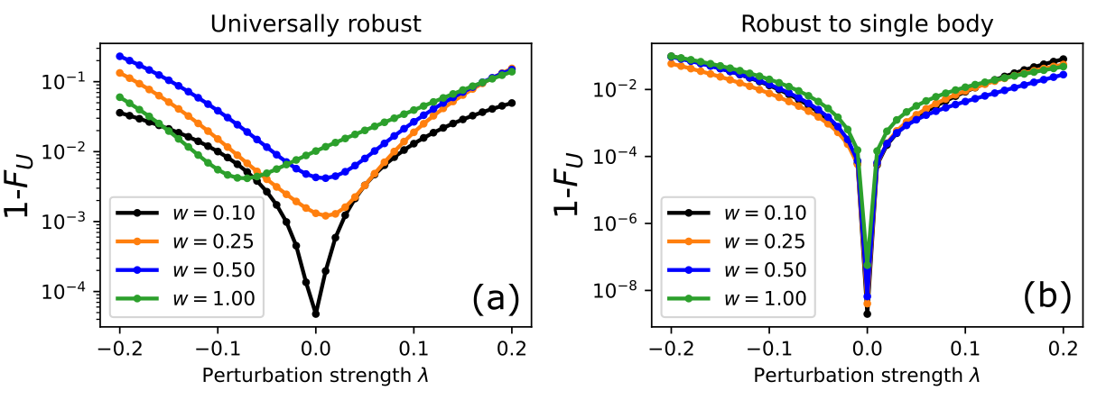
Figure S4: Analysis of the weight $w$ between targets in the numerical optimization, see Eq. (S75). Gate infidelity $1-F_{U}$ as a function of the perturbation strength. Results are shown for optimal control of two qubit gates (same case as shown in the main text) for the cases of (a) Universally robust and (b) Robust to single-body perturbations. Here $V=S_{z}$ and $\beta t_{f}=5$. See text for further details.

Finally we comment on the choice of the weight parameter $w$ in the optimization functional, i.e.,

$$\mathcal{J}_{\mathrm{URC}}\!=\!(J_{0}+wJ_{\mathrm{U}})/(1+w).$$ (S75)

For any $w$, the global minima is $\mathcal{J}_{\mathrm{URC}}=0$ which happens if and only if $J_{0}=0$ and $J_{\mathrm{U}}=0$. When any other solution is found, we would like that both targets are equally well achieved. We find that the straightforward choice of $w=1$ can put too much weight on the robustness requirement, in such a way that the ideal target fidelity found by the optimizer can be too high. This is seen in Fig. S4 (a), where we show the infidelity for the case of two-qubit gates (and random target unitary) when searching for gates that are universally robust. From the data, it can be seen that the fidelity at zero perturbation $\lambda=0$ can be quite high for relatively high values of $w$. This is because the optimizer is not able to get $J_{U}$ down to values which are of the order of the required infidelities. We expect that this can be improved by allowing more control time, but we leave a more detailed analysis for future work. For a fixed control time, this behavior can be adjusted by lowering the value of $w$. We point out that easier cases, for example the two-qubit case with robustness to only single-body operator, typically don’t have a strong dependence on the value of $w$, see Fig. S4 (b).