The VANDELS ESO public spectroscopic survey:
The spectroscopic measurements catalogue

VANDELS is a deep spectroscopic survey, performed with the VIMOS instrument at VLT, aimed at studying in detail the physical properties of high-redshift galaxies. VANDELS targeted $\sim$2100 sources at $1<z<6.5$ in the CANDELS Chandra Deep-Field South (CDFS) and Ultra-Deep Survey (UDS) fields. In this paper we present the public release of the spectroscopic measurement catalogues from this survey, featuring emission and absorption line centroids, fluxes, and rest-frame equivalent widths obtained through a Gaussian fit, as well as a number of atomic and molecular indices (e.g. Lick) and continuum breaks (e.g. D4000), and including a correction to be applied to the error spectra. We describe the measurement methods and the validation of the codes that were used.

1 Introduction

A major theme in extragalactic astronomy is understanding when and how galaxies formed and evolved. Spectroscopic surveys play a fundamental role in this respect, not only because they provide robust redshifts, but especially because the analysis of emission and absorption lines and spectral breaks grants access to intrinsic physical properties of galaxies such as the chemical composition of their gas and stellar populations, the ionising radiation field, and the gas and star kinematics.

Over the past two decades, several multi-slit and multi-fibre surveys have been carried out, targeting increasingly distant galaxies: from the Sloan Digital Sky Survey (SDSS) in the local Universe (Abazajian et al., 2003; Abdurro’uf et al., 2022), passing through the VIMOS VLT Deep Survey (VVDS; Le Fèvre et al., 2013; Garilli et al., 2008), zCOSMOS (Lilly et al., 2007), VIMOS Public Extragalactic Redshift Survey (VIPERS; Guzzo et al., 2014; Scodeggio et al., 2018), and the Large Early Galaxy Census (LEGA-C; van der Wel et al., 2016) at $<z>\sim 0.7$, the Galaxy Mass Assembly ultradeep Spectroscopic Survey (GMASS; Cimatti et al., 2008; Kurk et al., 2013) at Cosmic Noon, and up to $z\sim 4-6$ with KBSS-MOSFIRE (Steidel et al., 2014) and the VIMOS Ultra Deep Survey (VUDS; Le Fèvre et al., 2015), along with a number of smaller samples targeting the re-ionisation epoch (e.g. Pentericci et al., 2018b). All these surveys have improved our understanding of galaxy evolution, mainly by drawing a detailed 3D map of the Universe with thousands of redshifts.

VANDELS is an ESO public VIMOS survey of the Chandra Deep-Field South (CDFS) and Ultra-Deep Survey (UDS) fields that was designed to complement and extend the work of the CANDELS (Grogin et al., 2011; Koekemoer et al., 2011) imaging campaigns. The strategy of VANDELS was not to limit itself to finding a redshift, but to focus on ultra-long exposures of a relatively small number of galaxies that provide high signal-to-noise ratio (S/N) spectra to study in detail the physical characteristics of the high-redshift galaxies (McLure et al., 2018). Since the first data release of VANDELS (Pentericci et al., 2018a), a number of papers have been published studying several properties, ranging from dust attenuation, interstellar medium properties, and stellar metallicities of star-forming (Cullen et al., 2018, 2019; Calabrò et al., 2021; Fontanot et al., 2021; Calabrò et al., 2022a, b) and quiescent galaxies (Carnall et al., 2019, 2020, 2022; Hamadouche et al., 2022; Tomasetti et al., 2023; Hamadouche et al., 2023), to intergalactic medium properties (Thomas et al., 2020, 2021), the ionising photon production efficiency (Castellano et al., 2023), the LyC escape fraction (Begley et al., 2022; Saldana-Lopez et al., 2023), Ly$\alpha$, HeII$\lambda$1640, CIV$\lambda$1550, and CIII]$\lambda$1908 emitters (Marchi et al., 2019; Hoag et al., 2019; Cullen et al., 2020; Saxena et al., 2020a, b; Guaita et al., 2020; Saxena et al., 2022; Llerena et al., 2022; Mascia et al., 2023), AGN (Magliocchetti et al., 2020), and high-mass X-ray binaries (Saxena et al., 2021).

This paper represents the official release of the the VANDELS spectroscopic measurements (i.e. lines, indices, and breaks), which are herewith made available to the whole astrophysical community. The catalogues include all spectra from the VANDELS final data release (DR4) presented in Garilli et al. (2021) with a robust spectroscopic redshift.

The paper is organised as follows: Section 2 briefly describes the VANDELS survey; Section 3 summarises the methods of measurements; Section 4 discusses the measurement code validation tests, including a description of the creation of ad hoc mock 1D spectra; Section 5 discusses an issue with the error spectra and its resolution; Section 6 describes the released catalogues and the comparison with independent measurements from previously published works inside the VANDELS collaboration; and Section 7 provides a brief summary. In this paper, we provide magnitudes in the AB photometric system (Oke & Gunn, 1983).

Figure 1: Redshift distribution of the final VANDELS sample: the grey histogram includes all measurements, and the green histogram includes only reliable redshifts (confidence flag ¿ 1; see the text for more details).

2 The VANDELS survey

VANDELS is a spectroscopic survey performed with the ESO-VLT VIMOS spectrograph in two CANDELS fields, over a total area of $\sim$ 0.2 square degree. For all the details on the survey design, target selection, observations, data reduction, and spectroscopic redshift measurements, we refer the reader to McLure et al. (2018); Pentericci et al. (2018a); Garilli et al. (2021).

The VANDELS spectra cover a wavelength range of 4800 Å$<\lambda_{obs}<$ 9800 Å, with a dispersion of 2.5 Å/pixel and a spectral resolution of $R\sim 650$, corresponding to a FWHM${}_{res}\sim$ 460 km/s (or FWHM${}_{res}\sim$ 11.2 Å  at 7300 Å). The main targets of the survey were massive passive galaxies at $1<z<2.5$, bright star-forming galaxies (SFGs) at $2.4<z<5.5$, and fainter SFGs at $3<z<7$ Lyman-break galaxies, plus a small sample of AGN, pre-selected using various multi-wavelength criteria. The VANDELS spectroscopic targets were pre-selected using high-quality photometric redshifts and were observed for a minimum of 20 hrs and up to 80 hrs, depending on their brightness, in order to ensure an approximately homogeneous S/N on the continuum within each class of galaxy. The data reduction was carried out using the recipes provided by the VIMOS Interactive Pipeline and Graphical Interface (VIPGI) package (Scodeggio et al., 2005) and the EASYLIFE environment (Garilli et al., 2012). The measured S/N per resolution element is higher than ten for all passive and star-forming galaxies, and higher than five for 85% of Lyman-break galaxies and AGN (Garilli et al., 2021). Spectroscopic redshifts were determined for all objects using the Easy redshift (EZ) software package within the PANDORA environment (Garilli et al., 2010).

Table 1: slinefit parameters.

Parameter	Value	Description
dz	0.002	Range of redshifts to explore around the input value
delta_z	0.5	Step in the grid of redshifts, given as the fraction of one pixel
delta_width	0.5	Step in the grid of line widths ($\sigma$), given as the fraction of one pixel
delta_offset	0.5	Step in the grid of line offsets, given as the fraction of one pixel
num_mc	200	Number of random realisations of the spectrum to compute Monte Carlo uncertainties
width_min-width_max	50-500	Minimum and maximum allowed widths ($\sigma$) for a line [km/s]
same_width	false	Each line’s width is allowed (true) to vary freely and independently in the fit, or not (false)
offset_max	$\pm$1000	Maximum allowed velocity offset for lines [km/s]
offset_snr_min	3	Minimum S/N a line should have to be allowed to shift its centroid owing to velocity offsets

Table 2: Measured spectral lines (Gaussian fit).

Iona	Rest-frame	Iona	Rest-frame
	Wavelengthb ($\AA$)		Wavelengthb ($\AA$)
CIII	1175.5	CII]	2326.0
Ly$\alpha$	1215.7	FeII	2344.2
NV	1240.8	FeII-1	2374.5
SiII	1260.4	FeII-2	2382.8
OI+SiII	1303.3	NeIV	2421.8
CII	1334.5	FeII-1	2586.7
OIV	1341.6	FeII-2	2600.2
SiIV-1	1393.8	MgII-1	2796.4
SiIV-2	1402.8	MgII-2	2803.5
NIV	1486.5	MgI	2853.0
SV	1501.8	NeV	3425.9
SiII	1526.7	OII	3727.4
CIV	1549.5	H$\beta$	4861.3
FeII	1608.5	OIII-1	4958.9
HeII	1640.4	OIII-2	5006.8
OIII]	1666.1	NII-2	6548.0
AlII	1670.8	H$\alpha$	6562.8
AlIII-1	1854.7	NII-1	6583.5
AlIII-2	1862.8	SII-1	6716.4
CIII]	1908.7	SII-2	6730.8

• ^a Doublets are marked by the suffixes -1and -2.

• ^b Vacuum wavelengths are given for lines with $\lambda<3000\AA$; air wavelengths are given for lines with $\lambda>3000\AA$.

A redshift confidence flag was also assigned to each target, according to the following scheme, already applied to previous VIMOS surveys (e.g. VVDS, Le Fèvre et al., 2005; zCOSMOS, Lilly et al., 2007; VUDS, Le Fèvre et al., 2015).

• Flag 4: a highly reliable redshift (estimated to have a ¿ 99% probability of being correct), based on a high S/N spectrum and supported by obvious and consistent spectral features.

• Flag 3: also a very reliable redshift, comparable in confidence with Flag 4, supported by clear spectral features in the spectrum, but not necessarily with a high S/N.

• Flag 2: a fairly reliable redshift measurement, although not as straightforward to confirm as those for Flags 3 and 4, supported by cross-correlation results, continuum shape, and some spectral features.

• Flag 1: a reasonable redshift measurement, based on weak spectral features and/or continuum shape.
  An a posteriori analysis of the redshift reliability showed that the reliability of Flag 2 redshifts is $\sim$79%, while that of Flag 1 redshifts is  41% (Garilli et al., 2021).

• Flag 0: no reliable spectroscopic redshift measurement was possible.

• Flag 9: a redshift based on only one single clear spectral emission feature. An a posteriori analysis confirmed a redshift reliability of $\sim$ 95% for spectra with this flag.

• Flag -10: spectrum with clear problems in the observation or data-processing phases.

• Flag 10+any of the above: broad line AGN (BLAGN). This preliminary classification has been subsequently revised by Bongiorno et al. (in preparation).

• Serendipitous (also called secondary) objects appearing by chance within the slit of the main target were identified by adding a ’2’ in front of the main flag.

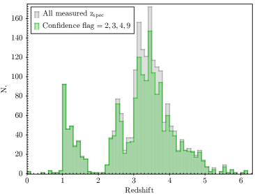
The redshift accuracy, estimated by internal comparison between different observations, is $\sigma_{\Delta z/(1+z)}$ = 0.0007 (Garilli et al., 2021). The redshift distribution of the entire VANDELS sample is shown in Fig. 1.

In the official catalogues, we include only the measurements for the 1811 objects with a reliable redshift confidence flag (2, 3, 4, and 9 and the equivalent for BLAGN and secondary objects), whose redshift distribution is also shown in Fig. 1.

We measured spectroscopic features using two methods: Gaussian fit and direct integration.

3 Gaussian fit measurements

Gaussian fit measurements were performed using slinefit (Schreiber et al., 2018), an automated code that models the observed spectrum of a galaxy as a combination of a stellar continuum model and a set of emission and absorption lines.

3.1 slinefit parameters

A set of templates from EAzY (Brammer et al., 2008), based on the Bruzual & Charlot (2003) stellar population models, is linearly combined to best fit the continuum. Table 1 summarises the parameters that were set to produce the official VANDELS catalogue. The code searches for lines around their expected locations given by the input redshift: lines with a S/N lower than offset_snr_min are fixed at their expected position, while a velocity offset with respect to the measured redshift is allowed for lines with a higher S/N, with a maximum value set by the offset_max parameter. We stress that in the catalogue the $\sigma$ of each line is provided, not the FWHM.

We measured 40 individual lines, including 7 resolved doublets, which are listed in Table 2. Unresolved doublets (e.g. CIV$\lambda$1550 and CIII]$\lambda$1908) were treated as a single line. For the NII$\lambda\lambda$6548,6583 and SII$\lambda\lambda$6716,6730 doublets, we fixed the line flux ratios to 0.33:1 and 1:0.75, respectively, while no constraints were imposed for the other doublets. All lines were modelled as single symmetric Gaussians, either in emission or in absorption. This might not have been the best choice for the Ly$\alpha$ line, which typically is asymmetric and sometimes even split into a blue and a red component. Therefore, after visual inspection of the spectra by four members of the team, we added a flag indicating whether the fit was good (1) or not (0) and recommend using with caution the Ly$\alpha$ parameters from the catalogue in the latter cases. In general, in the case of multi-component lines (e.g. P-Cygni profiles), only the strongest feature is fitted. We stress that slinefit, in our chosen configuration, always provides a solution. Therefore, we recommend caution when using spectral parameters when the lines are narrower than the spectral resolution (i.e. FWHM$\sim$460 km/s, corresponding to $\sigma\sim$195 km/s), because it might be a noise spike. Also, when the flux S/N$\leq$1, the line should be considered as undetected and the error on the flux can be used as a $1\sigma$ upper limit. Errors were evaluated through a Monte Carlo technique: the galaxy spectrum was randomly perturbed according to its re-scaled error spectrum (see the next Section) and the uncertainties on the spectroscopic parameters were then computed from the standard deviation of num_mc realisations of the fit.

Figure 2: Construction of the 1D mock spectra for the slinefit code validation. Top: Synthetic rest-frame template (from Talia et al. (2012)), normalised to unity at 1750Å. Bottom: Comparison between three examples of mock 1D spectra and real VANDELS spectra. Mock spectra are shown in black. VANDELS spectra are colour-coded with respect to their depth: 20hrs (red), 40hrs (green), and 80hrs (blue).

Figure 3: Comparison between slinefit results and input values for the sample of 270 mock spectra. In the top panels, we plotted the pull distributions. As a reference, we marked with a grey curve a Gaussian with a null mean and unity sigma. In the bottom panels, we plotted the relative change of the measured spectral quantities, with respect to their input values, as a function of the peak S/N of the lines. Black squares represent the median values of the relative change in bins of the S/N; error bars are the semi-interquartile range (SIQR). The line parameters are, starting clockwise from the top left figure: line centroid, EW, FWHM, and flux.

3.2 Mock 1D spectra and slinefit code validation

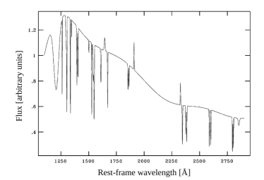
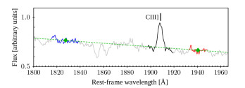
In order to validate the slinefit code performance, we built a set of 1D mock spectra to mimic the characteristics of the observed VANDELS ones. We started from a rest-frame template, normalised to unity at 1750Å  and created using the stacked spectrum of SFGs at z$\sim$2 from Talia et al. (2012) as reference (Fig. 2, top). The continuum was modelled as a cubic spline, with a slope of $\beta\sim$-1.1 and a dispersion of 1Å/pix. Emission and absorption spectral lines that are common in the UV range of SFG spectra (Table 2) were added as symmetric Gaussians. The lines were not all added at their vacuum rest-frame wavelength: some shifts were introduced in order to mimic the effects of outflows. We created three templates with the same continuum and varying the lines’ peak S/N in the range 0.3–7. Then, each rest-frame template was used to create 30 redshifted templates, with redshifts evenly distributed in the range 2.2–5.

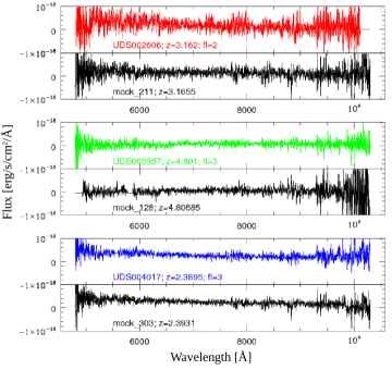
The redshifted templates were normalised to the F814W observed magnitude, following the magnitude versus redshift relation of the VANDELS survey. They were then re-sampled and cut to the VANDELS dispersion and observed wavelength range.

In order to add realistic noise, we extracted 1D spectra from empty regions in observed 2D spectra from the VANDELS survey at different exposure times and added them to the redshifted templates. The final validation sample counts 270 mock spectra. In Fig. 2 (bottom) we show the comparison between three examples of mock 1D spectra and real VANDELS spectra at different redshifts and with different quality flags.

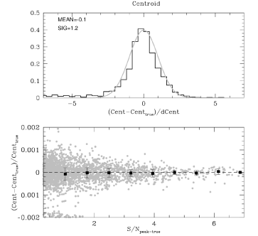
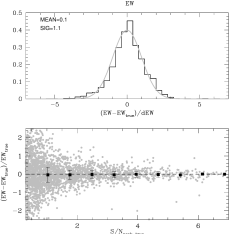
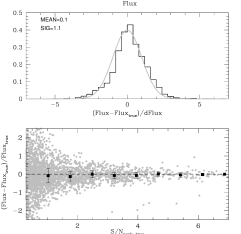
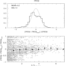
Finally, we ran the slinefit on the sample of mock 1D spectra with different sets of input parameters and checked the relative change in the measured spectral quantities with respect to their input values, and the pull distributions. In Fig. 3 we show the results from the run with the best set of parameters, which is summarised in Table 1. All the measured lines are included in the plots, but we stress that separating emission and absorption lines does not change the results. All distributions are consistent with a Gaussian with a null mean and unity sigma.

Figure 4: Median composite spectrum of VANDELS sources (grey). The upper and lower panels show zoomed-in regions around the HeII$\lambda$1640+OIII]$\lambda$1666 and CIII]$\lambda$1909 lines, respectively. The central bandpasses, as indicated in Table 3, are marked in black, while the two local continuum windows are marked in blue and red. The green points and dashed lines indicate the mean flux in the continuum bandpasses and the linear pseudo-continuum.

4 Direct integration

The direct integration measurements were performed using pylick , a flexible Python tool to measure spectral indices and associated uncertainties. The code is described in Borghi et al. (2022) and was extensively tested using spectra and results from the LEGA-C survey (van der Wel et al., 2016; Straatman et al., 2018). Following the approach of the Lick group (Worthey & Ottaviani, 1997), the code computes the strengths of a set of atomic and molecular indices and continuum breaks such as the D4000 (Bruzual A., 1983). Errors are evaluated following the S/N method by Cardiel et al. (1998).

Figure 5: Examples illustrating the four Ly$\alpha$ categories from Kornei et al. (2010). Clockwise, from the top left: emission, combination, absorption, and noise.

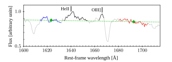
In our catalogue, we have included 55 indices and breaks defined in previous works, to which we added three UV emission line indices (see Table 3). The new indices were defined on the basis of a high-S/N composite spectrum of all VANDELS sources with a high-redshift quality flag (i.e. 3 and 4). It was built by median stacking the de-redshifted, scaled (by the median flux in the wavelength range 1410–1510 Å), and rebinned (0.6 Å/pix) spectra. In Fig. 4 we show the zoomed-in regions around the HeII$\lambda$1640+OIII]$\lambda$1666 and CIII]$\lambda$1909 lines, with the central bandpass and pseudo-continuum ranges marked in different colours. It should be noted that for the direct integration catalogue, no offset of the bandpasses is allowed with respect to the expected wavelength, given the redshift.

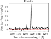
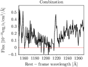
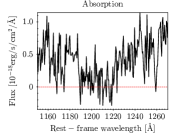
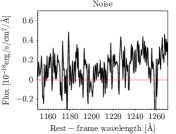
For the Ly$\alpha$ line, we opted for a different approach. Following Cullen et al. (2020), we applied the method by Kornei et al. (2010) to measure the EW of the line, which takes into account the line’s morphology to optimise the wavelength range over which the flux is integrated. The Ly$\alpha$ line of the 1218 individual galaxies at z$\gtrsim$2.95 (i.e. the redshift limit for the Ly$\alpha$ to be in the VIMOS wavelength range) was visually classified as either emission, absorption, combination, or noise; examples are shown in Fig. 5. The emission spectra are clearly dominated by a Ly$\alpha$ emission feature. The absorption spectra are dominated by an extended trough around the Ly$\alpha$ position. In the combination case, the spectrum contain superimposed emission and absorption features. Finally, the noise category include spectra where no clear feature could be identified at the Ly$\alpha$ position (see Kornei et al., 2010, for a detailed description). In the first three cases, after the peak of the emission and absorption, the integration window is defined by the wavelength values on either side of the peak where the flux intersects the average continuum level. The blue and red continua are defined as the median flux values in the range $\lambda$=[1120–1180]Å  and [1228–1255]Å, respectively. In the case of absorption and combination sources, the spectra were first smoothed with a boxcar function of six pixels in width to minimise the possibility of noise spikes affecting the determination of the boundaries of the integration range. For noise sources, the Ly$\alpha$ flux is simply defined as the integrated flux in the range $\lambda$=[1200–1228]Å. In all cases the line flux was divided by the red continuum value to obtain the EW.

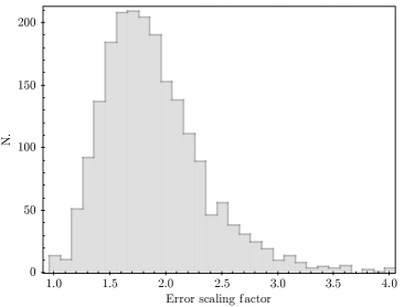
5 Scaling of the error spectra

The spectra distributed as part of the VANDELS public data release include the 1D noise estimate in erg cm^-2 s^-1 Å^-1. The error spectrum is a direct product of the data reduction procedures (Garilli et al., 2021), and should reflect the noise level of the corresponding object spectrum. However, the comparison between the error spectra and the noise r.m.s. of the object spectra, measured in line-free regions, shows a discrepancy, with the error spectra underestimating the noise level by a factor of $\sim$2, on average. We performed several tests on 2D and 1D spectra: our hypothesis is that the discrepancy is caused by the fact that the data reduction pipeline does not take the full covariance matrix into account. We opted for an a posteriori statistical correction of the error spectra (e.g. van der Wel et al. (2021)). In particular, for each object, we computed a scaling factor to be applied to the error spectrum. The scaling factor is defined as the standard deviation of the fit residuals, divided by the error spectrum:

$$1.482\times MAD[(object_{spectrum}-model_{spectrum})/error_{spectrum}],$$

where model_spectrum is the output of slinefit and MAD is the median absolute deviation. If the error spectrum is an accurate representation of the noise in the object spectrum, the above quantity should be close to 1; if the error spectrum underestimates the noise, then the above quantity can be used as a scaling factor. We computed it in five wavelength windows, free of strong sky lines, and then defined the scaling factor as the mean of the five values. The associated uncertainty is the error on the mean, which takes into account a slight wavelength dependence of the ratio between the noise r.m.s. of the object spectrum and the error spectrum (i.e. the ratio is on average $\sim$10$\%$ lower close to the spectral edges than in the central region). Fig. 6 shows the distribution of the scaling factor.

The slinefit code can actually perform the scaling of the error spectrum internally. If the appropriate keyword (residual_rescale) is switched on, the previously defined scaling factor is computed locally for each line; then, the whole error spectrum is normalised by interpolating between the scaling factors of the chosen lines, and the whole fit is performed a second time. The measurements in the official catalogue were instead performed by applying a single scaling factor to each error spectrum before running slinefit with the residual_rescale keyword switched off. This choice allowed us to provide a set of measurements that could be easily reproduced by other codes that do not include a scaling feature. The direct integration measurements were also performed after scaling the error spectra.

The scaling factors and their uncertainties are included in both catalogues. We stress that the error spectra in the VANDELS data release (i.e. NOISE extension or ERR column) are not scaled: they have to be multiplied by the scaling factor in order to obtain reliable errors on the spectroscopic measurements.

Table 3: pylick spectral indices.

Index	Central Bandpass	Blue Continuum	Red Continuum	Units	Type	Ref.a
BL1302	1292.000–1312.000	1270.000–1290.000	1345.000–1365.000	Å	atomicb	3
OI+SiII1303	1290.000–1307.000	1268.000–1286.000	1308.000–1324.000	Å	atomic	9
CII1335	1326.000–1340.000	1308.000–1324.000	1348.000–1378.000	Å	atomic	9
SiIV1400	1380.000–1407.000	1348.000–1378.000	1433.000–1460.000	Å	atomic	this workf
SiIV	1387.000–1407.000	1345.000–1365.000	1475.000–1495.000	Å	atomic	3
BL1425	1415.000–1435.000	1345.000–1365.000	1475.000–1495.000	Å	atomic	3
Fe1453	1440.000–1466.000	1345.000–1365.000	1475.000–1495.000	Å	atomic	3
SiII1526	1521.000–1533.000	1460.000–1495.000	1572.000–1599.000	Å	atomic	this workf
C${}_{IV}^{A}$	1530.000–1550.000	1500.000–1520.000	1577.000–1597.000	Å	atomic	3
CIV	1540.000–1560.000	1500.000–1520.000	1577.000–1597.000	Å	atomic	3
C${}_{IV}^{E}$	1550.000–1570.000	1500.000–1520.000	1577.000–1597.000	Å	atomic	3
FeII1608	1600.000–1616.000	1583.000–1599.000	1614.000–1632.000	Å	atomic	this workf
BL1617	1604.000–1630.000	1577.000–1597.000	1685.000–1705.000	Å	atomic	3
HeII 1640	1634.000–1654.000	1614.000–1632.000	1680.000–1705.000	Å	atomic	this work
BL1664	1651.000–1677.000	1577.000–1597.000	1685.000–1705.000	Å	atomic	3
OIII] 1666	1663.000–1668.000	1614.000–1632.000	1680.000–1705.000	Å	atomic	this work
AlII1670	1663.000–1679.000	1614.000–1632.000	1680.000–1705.000	Å	atomic	9
BL1719	1709.000–1729.000	1685.000–1705.000	1803.000–1823.000	Å	atomic	3
BL1853	1838.000–1868.000	1803.000–1823.000	1885.000–1915.000	Å	atomic	3
AlIII1860	1840.000–1873.000	1815.000–1839.000	1932.000–1948.000	Å	atomic	9
CIII 1909	1897.000–1919.000	1815.000–1839.000	1932.000–1948.000	Å	atomic	this work
FeII2370	2334.000–2391.000	2267.000–2290.000	2395.000–2450.000	Å	atomic	9
FeII2402	2382.000–2422.000	2285.000–2325.000	2432.000–2458.000	Å	atomic	3
BL2538	2520.000–2556.000	2432.000–2458.000	2562.000–2588.000	Å	atomic	3
FeII2600	2578.000–2611.000	2525.000–2572.000	2613.000–2674.000	Å	atomic	9
FeII2609	2596.000–2622.000	2562.000–2588.000	2647.000–2673.000	Å	atomic	3
B(2640)		2600.000–2630.000	2645.000–2675.000	dex	breakλc	7
MgII2800	2788.000–2810.000	2720.000–2785.000	2812.000–2842.000	Å	atomic	9
MgII	2784.000–2814.000	2762.000–2782.000	2818.000–2838.000	Å	atomic	3
MgI	2839.000–2865.000	2818.000–2838.000	2906.000–2936.000	Å	atomic	3
MgUV	2625.000–2725.000	2525.000–2625.000	2725.000–2825.000	dex	bumpd	4
Mgwide	2670.000–2870.000	2470.000–2670.000	2930.000–3130.000	Å	atomic	3
B(2900)		2855.000–2885.000	2915.000–2945.000	dex	breakλc	7
FeI	2965.000–3025.000	2906.000–2936.000	3031.000–3051.000	Å	atomic	3
BL3096	3086.000–3106.000	3031.000–3051.000	3115.000–3155.000	Å	atomic	3
CaII K	3925.650–3945.000	3845.000–3880.000	3950.000–3954.000	Å	atomic	8
CaII H	3959.400–3975.000	3950.000–3954.000	3983.000–3993.000	Å	atomic	8
D4000		3750.000–3950.000	4050.000–4250.000	dex	breakν	5
Dn4000		3850.000–3950.000	4000.000–4100.000	dex	breakν	6
H$\delta_{A}$	4083.500–4122.250	4041.600–4079.750	4128.500–4161.000	Å	atomic	2
H$\delta_{F}$	4091.000–4112.250	4057.250–4088.500	4114.750–4137.250	Å	atomic	2
CN1	4142.125–4177.125	4080.125–4117.625	4244.125–4284.125	mag	moleculare	1
CN2	4142.125–4177.125	4083.875–4096.375	4244.125–4284.125	mag	molecular	1
Ca4227	4222.250–4234.750	4211.000–4219.750	4241.000–4251.000	Å	atomic	1
G4300	4281.375–4316.375	4266.375–4282.625	4318.875–4335.125	Å	atomic	1
H$\gamma_{A}$	4319.750–4363.500	4283.500–4319.750	4367.250–4419.750	Å	atomic	2
H$\gamma_{F}$	4331.250–4352.250	4283.500–4319.750	4354.750–4384.750	Å	atomic	2
Fe4383	4369.125–4420.375	4359.125–4370.375	4442.875–4455.375	Å	atomic	1
Ca4455	4452.125–4474.625	4445.875–4454.625	4477.125–4492.125	Å	atomic	1
Fe4531	4514.250–4559.250	4504.250–4514.250	4560.500–4579.250	Å	atomic	1
C24668	4634.000–4720.250	4611.500–4630.250	4742.750–4756.500	Å	atomic	1
H$\beta$	4847.875–4876.625	4827.875–4847.875	4876.625–4891.625	Å	atomic	1
Fe5015	4977.750–5054.000	4946.500–4977.750	5054.000–5065.250	Å	atomic	1
Mg1	5069.125–5134.125	4895.125–4957.625	5301.125–5366.125	mag	molecular	1
Mg2	5154.125–5196.625	4895.125–4957.625	5301.125–5366.125	mag	molecular	1
Mgb	5160.125–5192.625	5142.625–5161.375	5191.375–5206.375	Å	atomic	1
Fe5270	5245.650–5285.650	5233.150–5248.150	5285.650–5318.150	Å	atomic	1
Fe5335	5312.125–5352.125	5304.625–5315.875	5353.375–5363.375	Å	atomic	1

• ^a 1: Trager et al. (1998); 2: Worthey & Ottaviani (1997); 3: Maraston et al. (2009); 4: Daddi et al. (2005); 5: Bruzual A. (1983); 6: Balogh et al. (1999); 7: Spinrad et al. (1997); 8: Fanfani (2019); 9: Leitherer et al. (2011).

• ^b Borghi et al. (2022) Eq. 1; ^c Borghi et al. (2022) Eq. 2; ^d Borghi et al. (2022) Eq. 4; ^e as Borghi et al. (2022) Eq. 4, but integrating over $F(\lambda)d\lambda$, instead of $F(\nu)d\nu$; ^f these indices were firstly defined by Leitherer et al. (2011), but here we present a slightly modified version.

Figure 6: Distribution of the multiplicative scaling factors to correct the mismatch between the error spectra and the noise of the object spectra.

Table 4: Legend of catalogue content.

#	Column name	Description	Units
Gaussian fit
1	objID	Object identification
2	z	Spectroscopic redshift
3	zQfl	Redshift confidence flag (Sec. 2)
4-5	scaling_factor, e_scaling_factor	Scaling factor (Sec. 5) (and error)
6	ly$\alpha$_fl	Goodness-of-fit flag for Ly$\alpha$ (Sec. 3)
7-406		Lines parameters from slinefit:
	wave, ewave	observed centroid wavelength (and error)	microns
	flux, eflux	lines flux (and error)	erg s-1 cm-2
	cont, econt	continuum flux (and error)	erg s-1 cm-2 Å-1
	ew, eew	rest-frame EWa (and error)	Å
	sigma, esigma	line widthb (and error)	km s-1
Direct integration
1	objID	Object identification
2	z	Spectroscopic redshift
3	zQfl	Redshift confidence flag (Sec. 2)
4-5	err_scaling_factor, eerr_scaling_factor	Error scaling factor (Sec. 5) (and error)
6	lya_class	Ly$\alpha$ visual classification (Sec. 4):
		1=emission; 2=combination; 3=absorption; 4=noise
7-8	LyA_EW0_K10, LyA_EW0_K10_err	Ly$\alpha$ EW following Kornei et al. (2010) (and error)	Å
		Indices/breaks from pylick:
9-182	index name, err	rest-frame EWa [atomic indices];	Å;
		rest-frame EW [molecular indices]; break (and error)	mag; unitless (Tab. 3)
	cont	Pseudo-continuum flux	erg s-1 cm-2 Å-1

• ^a EW sign convention: positive for emission lines; negative for absorption lines.

• ^b We stress that in the catalogue the Gaussian $\sigma$ of each line is provided, not the FWHM.

6 The catalogues

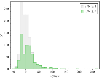
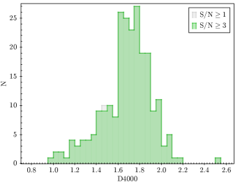
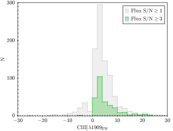
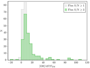
We have produced a total of four catalogues: two (one for each field) for the Gaussian fit measurements performed with slinefit and two (again, one for each field) for the direct integration measurements performed with pylick plus Ly$\alpha$ following the Kornei et al. (2010) method. The contents of the catalogues are summarised in Table 4, while in Fig. 7 we show the distributions of the EW of some notable lines and, for the passive galaxies’ sample at $z<2$, the D4000 break. As already mentioned, we computed spectral properties only for galaxies with a reliable redshift, namely those with a quality flag = 2,3,4,9. In the slinefit catalogue we have not included the measurements for the three BLAGN whose emission line fits require two components. Dedicated spectral measurements for these objects will be presented in Bongiorno et al. (in prep.).

Figure 7: Distributions of the D4000 break and the EW of some notable lines. In each panel we show the distributions at S/N$\geq$1 (light grey) and S/N$\geq$3 (green). For the lines from the ’Gaussian fit’ catalogues, the cut is in S/N flux. Top left: Ly$\alpha$ EW (direct integration). Top right: D4000 (direct integration), Middle left: CIII]$\lambda$1909Å  EW (Gaussian fit). Middle right: [OII]$\lambda$3727Å  EW (Gaussian fit). Bottom left: OI+SiII$\lambda$1303Å  EW (direct integration). Bottom right: OI+SiII$\lambda$1303Å  EW (Gaussian fit). In the last two panels, we also show the distribution at S/N$\geq$2 (dark grey).

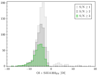
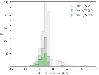
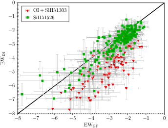
The EW of some lines was measured using both the Gaussian fit and direct integration methods. The agreement between the two measurements is very good in the case of single lines, as shown in Fig. 8 for the SiII$\lambda$1526Å, as an example: on average, the linear correlation coefficient is $r_{xy}\gtrsim{0.9}$ and the root-mean-square error (RMSE) is $\sim$0.5-0.6Å. A systematic small offset of $\lesssim$0.5Å  is attributable to the different ways of determining the continuum level in the two methods. In the case of unresolved groups of lines, where a single-Gaussian model was assumed (e.g. OI+SiII$\lambda$1303Å), the correlation coefficient between the two methods is still high ($r_{xy}\gtrsim{0.8}$, on average, with an RMSE of $\sim$0.7-0.8Å), but the Gaussian fit tends to systematically underestimate the flux, more than what would be expected by accounting only for the differences in the continuum. The EW ratio between the two methods is on average between 0.6 and 0.8, depending on the group of lines.

Figure 8: Examples of EW comparison between Gaussian fit and direct integration methods for a single line (SiII$\lambda$1526Å; red triangles) and an unresolved group of lines (OI+SiII$\lambda$1303Å; green squares). Only measurements at S/N$\geq$3 are shown. The 1-to-1 relation is also indicated in black.

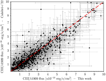
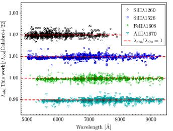
Finally, as an additional validation, in Fig. 9 we compare subsets of measurements from our catalogues to independent and previously published measurements performed with different codes and methods by VANDELS team members. For the Gaussian fit catalogue, we compared our measurements of the CIII]$\lambda$1909Å  flux and of the centroids of four absorption lines to those by Calabrò et al. (2022b), which were obtained by fitting each line profile with a Gaussian function using the Python version of the MPFIT routine (Markwardt, 2009). The continuum was parameterised as a straight line and fitted simultaneously with the lines. We find a good agreement between the two sets of measurements (no S/N cut applied): for the CIII]$\lambda$1909Å  fluxes, the linear correlation coefficient is $r_{xy}\sim{0.9}$ and the RMSE$\sim$0.8$\times$10^-18erg s^-1 cm², with no significant offset with respect to the 1-to-1 relation. On the other hand, for the absorption lines’ centroids $r_{xy}\sim{1.0}$ and RMSE$\sim$5.0$\times$10^-4Å.

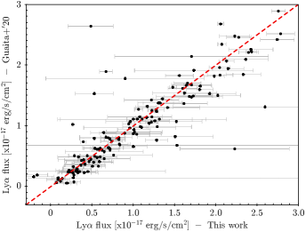
We checked the Ly$\alpha$ flux measurements from Guaita et al. (2020), which were obtained with a custom code based on the optimize.leastsq Python function (see also Guaita et al. (2017)), by fitting the lines with a Gaussian profile and assuming a linear continuum. Guaita et al. (2020) provide two sets of measurements: one assuming a symmetric Gaussian profile, the other using a skewed Gaussian function. For our exercise, we took the former set (i.e. symmetric Gaussian) and limited the comparison to the galaxies with a goodness-of-fit flag for Ly$\alpha$ equal to 1 (see Sec. 3). We also find in this case a good agreement between the two measurements, with an $r_{xy}\sim{0.9}$ and the RMSE$\sim$0.3$\times$10^-17erg s^-1 cm².

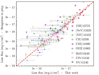
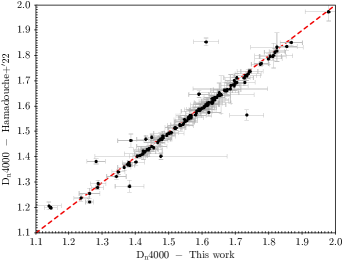
We compared our flux measurements for different emission lines in the VANDELS AGN sample (excluding BLAGN) to the ones obtained with a custom Python code from Bongiorno et al. (in prep.): the line fluxes are the mean of a Gaussian and a Lorentzian profile fit, plus a polynomial continuum. The $r_{xy}$ and RMSE range from 0.7 to 0.9 and from 2.0$\times$10^-17 to 4.0$\times$10^-17erg s^-1 cm², respectively, depending on the line. Finally, we checked the D_n4000 break in the VANDELS subsample of quiescent galaxies from our direct integration catalogue against the independent measurements by Hamadouche et al. (2022) and we found an excellent agreement ($r_{xy}\sim{1.0}$ and RMSE$\sim$3.0$\times$10^-2).

Figure 9: Comparison between the measurements presented in this work and previously published VANDELS results. In all plots we also show the one-to-one relation (dashed red line). Top left: CIII]$\lambda$1909Å  flux from Calabrò et al. (2022b) (Gaussian fit). Top right: interstellar medium absorption line centroids from Calabrò et al. (2022b) (Gaussian fit; the points for the different ions have been shifted by 0.01 for visualisation purposes). Middle left: Ly$\alpha$ flux from Guaita et al. (2020) (Gaussian fit; no error was available for these measurements). Middle right: AGN emission line flux from Bongiorno et al. (in prep.) (Gaussian fit). Bottom: D_n4000 from Hamadouche et al. (2022) (direct integration).

7 Summary

In this paper, we present the public release of the spectroscopic measurements of the VANDELS survey (Pentericci et al., 2018a; McLure et al., 2018; Garilli et al., 2021). We built two catalogues: one containing line properties from Gaussian fit measurements performed with the slinefit code, the other including line indices and continuum breaks measured with the pylick code, plus Ly$\alpha$ EWs following the Kornei et al. (2010) method. We created a set of mock spectra to mimic observed VANDELS sources in order to validate the slinefit code, while the pylick code was already tested in a previous work (Borghi et al., 2022). As a further check of the accuracy of our catalogues, we compared subsets of measurements to previous results obtained with different codes and methods. We have also found that the error spectra included in the VANDELS data release underestimate the noise level when compared to the r.m.s. of the object spectra and computed a correction that we provide in the catalogues. The full spectroscopic catalogues, together with the spectra, redshift catalogues, complementary photometric information, and SED fitting derived quantities, are publicly available from the VANDELS survey database and at the CDS.