Single-Antenna Jammers in MIMO-OFDM
Can Resemble Multi-Antenna Jammers

Abstract

In multiple-input multiple-output (MIMO) wireless systems with frequency-flat channels, a single-antenna jammer causes receive interference that is confined to a one-dimensional subspace. Such a jammer can thus be nulled using linear spatial filtering at the cost of one degree of freedom. Frequency-selective channels are often transformed into multiple frequency-flat subcarriers with orthogonal frequency-division multiplexing (OFDM). We show that when a single-antenna jammer violates the OFDM protocol by not sending a cyclic prefix, the interference received on each subcarrier by a multi-antenna receiver is, in general, not confined to a subspace of dimension one (as a single-antenna jammer in a frequency-flat scenario would be), but of dimension $L$, where $L$ is the jammer’s number of channel taps. In MIMO-OFDM systems, a single-antenna jammer can therefore resemble an $L$-antenna jammer. Simulations corroborate our theoretical results. These findings imply that mitigating jammers with large delay spread through linear spatial filtering is infeasible. We discuss some (im)possibilities for the way forward.

I Introduction

Jammers are a pervasive threat to wireless communication [1]. Linear spatial filtering in multiple-input multiple-output (MIMO) systems was shown to be effective in mitigating jammers and has been studied extensively; see, e.g.,[1, 2, 3]. Even though many modern wireless systems utilize orthogonal frequency-division multiplexing (OFDM) [4] to deal with frequency-selective wideband channels, the jammer-mitigation literature has focused mostly on frequency-flat channels [5, 6, 3, 7]. References [2, 8, 9, 10, 11, 12] consider frequency-selective channels with OFDM, but substitute a frequency-flat input-output model for each subcarrier where the (single-antenna) jammer is modeled as one-dimensional interference per subcarrier. However, to transform a frequency-selective channel into mutually orthogonal frequency-flat subcarriers, OFDM requires the transmitters to prepend a cyclic prefix to each OFDM symbol [4]. Since jammers are malicious, they might not send a cyclic prefix. This has been noted before [13, 14, 15], but the consequences of violating the cyclic prefix in MIMO-OFDM systems have not been analyzed and are unknown.

This letter fills this gap by showing that a single-antenna jammer that violates the cyclic prefix can appear as $L$-dimensional interference per subcarrier (i.e., like an $L$-antenna jammer), where $L$ is the jammer’s number of nonzero channel taps. The consequences are (i) that the common practice of modeling jammers as one-dimensional interference per OFDM-subcarrier is wrong and (ii) that mitigating jammers with large delay spread via linear spatial filtering is impractical. Possibilities for the way forward are discussed.

I-A Notation

We use uppercase boldface for matrices; $\mathbf{A}^{T}$ and $\mathbf{A}^{H}$ are the transpose and conjugate transpose of $\mathbf{A}$, respectively. Column vectors are denoted in two different ways: as lowercase boldface (e.g., $\mathbf{a}$), if they represent spatial vectors (e.g., corresponding to an antenna array), or as underlined lowercase boldface (e.g., $\underline{\mathbf{a}}$), if they represent vectors across time/frequency. Comma denotes horizontal concatenation (e.g., $[\mathbf{a},\mathbf{b}]$); semicolon denotes vertical concatenation (e.g., $[\mathbf{a};\mathbf{b}]$). A vector $\mathbf{a}\in\mathbb{C}^{N}$ in reverse order is denoted by its reflected letter $\reflectbox{$\mathbf{a}$}=[a_{N},\dots,a_{1}]^{T}$. The subspace spanned by $\mathbf{a}$ is $\text{span}(\mathbf{a})$; its orthogonal complement is $\text{span}(\mathbf{a})^{\perp}$. The $M\!\times\!N$ zero matrix is $\mathbf{0}_{M\times N}$ or $\mathbf{0}$. $\mathbf{F}_{N}$ is the unitary $N$-point discrete Fourier transform (DFT) matrix; $\oast$ denotes cyclic convolution. $\mathcal{C}\mathcal{N}(\mathbf{0},\mathbf{C})$ is the circularly-symmetric complex Gaussian distribution with covariance $\mathbf{C}$.

II Prerequisites

II-A MIMO Jammer Mitigation in Frequency-Flat Systems

In MIMO systems with frequency-flat channels, the input-output (I/O) relation between transmitter and receiver in presence of a single-antenna jammer can be modeled as

$$\mathbf{y}[k]=\mathbf{H}\mathbf{s}[k]+\mathbf{j}w[k]+\mathbf{n}[k].$$ (1)

Here, $\mathbf{y}[k]\in\mathbb{C}^{B}$ is the receive signal of a $B$-antenna receiver at sample instant $k$, $\mathbf{H}\in\mathbb{C}^{B\times U}$ is the frequency-flat channel matrix between the receiver and one or more transmitters with a total of $U$ antennas and transmit signal $\mathbf{s}[k]\in\mathbb{C}^{U}$, $\mathbf{j}\in\mathbb{C}^{B}$ is the frequency-flat channel of the jammer with transmit signal $w[k]\in\mathbb{C}$, and $\mathbf{n}[k]\sim\mathcal{C}\mathcal{N}(\mathbf{0},N_{0}\mathbf{I}_{B})$ models noise. We assume a block fading scenario so that $\mathbf{H}$ and $\mathbf{j}$ do not depend on $k$.

In (1), the receive interference is restricted to the one-dimensional subspace $\text{span}(\mathbf{j})\subset\mathbb{C}^{B}$. The receiver can therefore mitigate the jammer by projecting the receive signal onto the orthogonal complement $\text{span}(\mathbf{j})^{\perp}$ of $\text{span}(\mathbf{j})$. Specifically, let $\mathbf{u}_{1},\dots,\mathbf{u}_{B-1}\in\mathbb{C}^{B}$ be an orthonormal basis of $\text{span}(\mathbf{j})^{\perp}$, and let $\mathbf{U}\triangleq[\mathbf{u}_{1},\dots,\mathbf{u}_{B-1}]\in\mathbb{C}^{(B-1)\times B}$. Then, the receiver can project the receive signal onto $\text{span}(\mathbf{j})^{\perp}$ by computing

$$\bar{}\mathbf{y}[k] \triangleq\mathbf{U}^{H}\mathbf{y}[k]=\underbrace{\mathbf{U}^{H}\mathbf{H}}_{\triangleq\bar{}\mathbf{H}\in\mathbb{C}^{(B-1)\times U}}\mathbf{s}[k]~{}+~{}\underbrace{\mathbf{U}^{H}\mathbf{j}}_{=\mathbf{0}}w[k]+\underbrace{\mathbf{U}^{H}\mathbf{n}[k]}_{\triangleq\bar{}\mathbf{n}[k]}$$ (2)

$$=\bar{}\mathbf{H}\mathbf{s}[k]+\bar{}\mathbf{n}[k]\in\mathbb{C}^{B-1}.$$ (3)

Thus, the receiver can eliminate the jammer at the cost of one degree of freedom, obtaining a virtual jammer-free I/O relationship with channel matrix $\bar{}\mathbf{H}\in\mathbb{C}^{(B-1)\times U}$ and noise $\bar{}\mathbf{n}[k]\sim\mathcal{C}\mathcal{N}(\mathbf{0},N_{0}\mathbf{I}_{B-1})$. The following result is well-known:

Proposition 1.

In frequency-flat MIMO, the receive interference of single-antenna jammer is confined to a one-dimensional subspace and can be nulled at the cost of one degree of freedom.

The extension to multiple or multi-antenna jammers is straightforward: The receiver can completely null jammers with a channel matrix $\mathbf{J}$ at the cost of $\text{rank}(\mathbf{J})$ degrees of freedom.

II-B OFDM Basics

We give a short but rigorous derivation of OFDM that serves as a template for the proof of our main result in sec:main. OFDM is widely used for eliminating inter-symbol interference (ISI) that results from high symbol-rate communication over frequency-selective wideband channels [4]. OFDM exploits the fact that the DFT matrix diagonalizes circulant matrices (i.e., if $\mathbf{C}$ is circulant, then $\mathbf{F}_{N}\mathbf{C}\mathbf{F}_{N}^{H}$ is diagonal) to partition a wideband channel into multiple frequency-flat narrowband subcarriers. The subcarriers are orthogonal and can be treated independently, without need for complex equalization techniques.

Specifically, consider a discrete-time single-input single-output (SISO) system in which the channel impulse response has length $L$ and is denoted by $\underline{\mathbf{h}}=[h[1],\dots,h[L]]^{T}$. If the transmitter transmits an information-carrying sequence $\underline{\mathbf{x}}=[x[1],\dots,x[N]]^{T}$, then the channel output is a length-$(N+L-1)$ sequence $\underline{\mathbf{y}}=[y[1],\dots,y[N+L-1]]^{T}$ given by

$$\begin{bmatrix}y[1]\\ \vdots\\ y[N\!+\!L\!-\!1]\end{bmatrix}=\begin{bmatrix}h[1]&0&&\cdots&0\\[-2.84526pt] &\ddots&&&\vdots\\[-2.84526pt] 0&\cdots&~{}\underline{\reflectbox{$\mathbf{h}$}}^{T}&\cdots&0\\[-2.84526pt] \vdots&&&\ddots&\vdots\\[-2.84526pt] 0&\cdots&&0&h[L]\end{bmatrix}\begin{bmatrix}x[1]\\ \vdots\\ x[N]\end{bmatrix}+\underline{\mathbf{n}},$$ (4)

where the entries of the noise $\underline{\mathbf{n}}$ are i.i.d. $\mathcal{C}\mathcal{N}(0,N_{0})$ distributed.

In OFDM, the transmitter does not simply transmit the information-carrying sequence $\underline{\mathbf{x}}$. Instead, it prepends a so-called cyclic prefix of length $P\geq L-1$, which consists of the last $P$ symbols of $\underline{\mathbf{x}}$. That is, the transmitter does not transmit the length-$N$ sequence $\underline{\mathbf{x}}$ but the length-$(N+P)$ sequence $\tilde{\underline{\mathbf{x}}}=[x[N\!-\!P\!+\!1],\dots,x[N],x[1],x[2],\dots,x[N]]^{T}$. The sequence $\tilde{\underline{\mathbf{x}}}$ is called an OFDM symbol. Analogous to (4), the receive sequence associated to an OFDM symbol has length $N+P+L-1$. The receiver discards the first $P$ of these receive symbols (which correspond to the cyclic prefix) as well as the last $L-1$ receive symbols (which correspond to the reverberation of the channel impulse response, cf. (4)). What remains is a length-$N$ sequence $\underline{\tilde{}\mathbf{y}}=[\tilde{y}[1],\dots,\tilde{y}[N]]^{T}$ whose dependence on the transmit signal can be written as

$$\!\!\!\!\begin{bmatrix}\tilde{y}[1]\\ \vdots\\ \tilde{y}[N]\end{bmatrix} =\begin{bmatrix}0&\cdots~{}0&&\reflectbox{\text@underline{$\mathbf{h}$}}^{T}&0&&\cdots&0\\[-2.84526pt] &&&&\ddots&&&\vdots\\ &&&&0&\reflectbox{\text@underline{$\mathbf{h}$}}^{T}&0&\\[-2.84526pt] \vdots&&&&&&\ddots&\vdots\\ 0&\cdots&&&&&0&\reflectbox{\text@underline{$\mathbf{h}$}}^{T}\end{bmatrix}\tilde{\underline{\mathbf{x}}}+\underline{\mathbf{n}}$$ (5)

$$=\begin{bmatrix}h[1]&0&\cdots&0&h[L]&\cdots&&h[2]\\ h[2]&h[1]&\cdots&0&0&h[L]&\cdots&h[3]\\[-2.84526pt] &&\ddots&&\\[-2.84526pt] 0&\cdots&&&h[L]&\lx@intercol\hfil\cdots\hfil\lx@intercol&h[1]\end{bmatrix}\begin{bmatrix}x[1]\\ \vdots\\ x[N]\end{bmatrix}\!+\underline{\mathbf{n}},\!$$ (6)

where the step from (5) to (6) exploits the cyclic prefix of $\tilde{\underline{\mathbf{x}}}$. (In (5), the $P-L+1$ first columns of the matrix are zero.) Since the matrix in (6) is circulant, we can also write (6) as a cyclic convolution with the channel impulse response:

$$\underline{\tilde{}\mathbf{y}}=\underline{\mathbf{h}}\oast\underline{\mathbf{x}}+\underline{\mathbf{n}}.$$ (7)

By defining $\hat{\underline{\mathbf{y}}}=\mathbf{F}_{N}\underline{\tilde{}\mathbf{y}}$, $\hat{\underline{\mathbf{h}}}=\mathbf{F}_{N}[\underline{\mathbf{h}};\mathbf{0}_{(N-L)\times 1}]$, $\hat{\underline{\mathbf{x}}}=\mathbf{F}_{N}\underline{\mathbf{x}}$, and $\hat{\underline{\mathbf{n}}}=\mathbf{F}_{N}\underline{\mathbf{n}}$, we can restate (7) in the frequency domain as

$$\hat{\underline{\mathbf{y}}}=\sqrt{N}\text{diag}(\hat{\underline{\mathbf{h}}})\,\hat{\underline{\mathbf{x}}}+\hat{\underline{\mathbf{n}}}.$$ (8)

So if the transmitter sets the information-carrying sequence $\underline{\mathbf{x}}$ to the inverse DFT of the symbol sequence $\underline{\mathbf{s}}=[s[1],\dots,s[N]]^{T}$, $\underline{\mathbf{x}}=\mathbf{F}_{N}^{H}\underline{\mathbf{s}}$, and if the receiver ignores the first $P$ receive symbols and computes the DFT of the next $N$ receive symbols, $\hat{\underline{\mathbf{y}}}=\mathbf{F}_{N}\underline{\tilde{}\mathbf{y}}$, then the resulting I/O relation can be stated as

$$\hat{\underline{\mathbf{y}}}=\sqrt{N}\text{diag}(\hat{\underline{\mathbf{h}}})\,\underline{\mathbf{s}}+\hat{\underline{\mathbf{n}}}.$$ (9)

Note the absence of ISI in (9), which consists of $N$ scalar I/O relations that correspond to $N$ OFDM subcarriers. These subcarrier I/O relations can also be stated individually as

$$\hat{y}[k]=\sqrt{N}\hat{h}[k]s[k]+\hat{n}[k],\quad k=1,\dots,N.$$ (10)

This SISO-OFDM template can be applied analogously for SIMO or MIMO systems, where the I/O relation for the $k$th subcarrier is

$$\bm{\hat{}}\mathbf{y}[k]=\sqrt{N}\bm{\hat{}}\mathbf{h}[k]\mathbf{s}[k]+\bm{\hat{}}\mathbf{n}[k],\quad k=1,\dots,N,$$ (11)

and

$$\bm{\hat{}}\mathbf{y}[k]=\sqrt{N}\bm{\hat{}}\mathbf{H}[k]\mathbf{s}[k]+\bm{\hat{}}\mathbf{n}[k],\quad k=1,\dots,N,$$ (12)

respectively, and where the individual entries of $\bm{\hat{}}\mathbf{h}[k]$ and $\bm{\hat{}}\mathbf{H}[k]$ correspond to the $k$th subcarrier between the individual transmit and receive antennas. In both cases, the I/O relation between the individual transmit and receive antennas has the form of (10). However, OFDM relies on the transmitter(s) to send a cyclic prefix that enables treating the convolution (5) as a cyclic convolution (7) and to diagonalize it using a DFT matrix.

III Main Result

If a single-antenna jammer were to comply with OFDM by sending a cyclic prefix, then (and only then) the per-subcarrier I/O relation of a MIMO-OFDM system would have the form

$$\bm{\hat{}}\mathbf{y}[k]=\sqrt{N}\bm{\hat{}}\mathbf{H}[k]\mathbf{s}[k]+\sqrt{N}\bm{\hat{}}\mathbf{j}[k]w[k]+\bm{\hat{}}\mathbf{n}[k]$$ (13)

for $k=1,\dots,N$ (with $\bm{\hat{}}\mathbf{j}[k]$ being the $k$th subcarrier of the jammer’s channel to the receiver), which is structurally equivalent to the frequency-flat I/O relation in (1). The receive interference would be confined to a one-dimensional subspace and could be nulled at the cost of one degree of freedom.

By nature, however, jammers are malicious—if they can gain an advantage from violating the cyclic prefix, they will do so. The question is how the absence of a cyclic prefix affects the per-subcarrier I/O relation of a MIMO-OFDM system under a jamming attack. The answer is the main result of this letter. To formally state the result, we assume that the channel impulse response between the single-antenna jammer and the $B$-antenna receiver consists of $L$ nonzero taps $\mathbf{j}[1],\dots,\mathbf{j}[L]\in\mathbb{C}^{B}$.

Theorem 1.

The per-subcarrier receive interference caused by a single-antenna jammer that attacks a MIMO-OFDM system without sending a cyclic prefix spans a subspace whose dimension can be up to $\min\{B,L\}$.

Proof.

There are two cases: In the case $L>B$, the dimension of the interference subspace is trivially bounded by the number of receive antennas $B$, and thus by $\min\{B,L\}$. The other case is the case $L\leq B$, for which we will prove that the dimension of the interference subspace is bounded by $L$, and thus by $\min\{B,L\}$. To analyze the receive interference of a single-antenna jammer, we can ignore noise as well as signals sent by the legitimate transmitter. We use $\underline{\mathbf{j}}_{b}=[j_{b}[1],\dots,j_{b}[L]]^{T}$ to denote the channel impulse response from the jammer to the $b$th receive antenna, $b=1,\dots,B$.

We assume that the attacked communication system (but not the jammer!) uses an OFDM scheme with $N$ subcarriers and a cyclic prefix of length $P\geq L-1$. In accordance with OFDM, the BS aggregates (per antenna) the receive symbols that correspond to an OFDM symbol while discarding the portions that correspond to the cyclic prefix and to the reverberation of the channel impulse response. We can thus write the receive signal at the $b$th antenna corresponding to an OFDM symbol as

$$\begin{bmatrix}y_{b}[1]\\ \vdots\\ y_{b}[N]\end{bmatrix}=\begin{bmatrix}0~{}&\cdots&0~{}&\reflectbox{\text@underline{$\mathbf{j}$}}_{b}^{T}&0&\cdots&0\\ \vdots&&&0&\reflectbox{\text@underline{$\mathbf{j}$}}_{b}^{T}&\cdots&0\\ &&&&&\ddots&\vdots\\ 0&&&&\cdots&0&\reflectbox{\text@underline{$\mathbf{j}$}}_{b}^{T}\end{bmatrix}\begin{bmatrix}w[-P+1]\\[-5.69054pt] \vdots\\ w[0]\\ w[1]\\[-2.84526pt] \vdots\\ w[N]\end{bmatrix}$$ (14)

or, more compactly, as

$$\underline{\mathbf{y}}_{b} =\mathbf{J}_{b}\underline{\mathbf{w}}.$$ (15)

The matrix $\mathbf{J}_{b}\in\mathbb{C}^{N\times(N+P)}$ is Toeplitz and its first $P-L+1$ columns are zero. We now rewrite $\underline{\mathbf{w}}=[\underline{\mathbf{w}}^{(\textsf{p})};\underline{\mathbf{w}}^{(\ast)}]$, where $\underline{\mathbf{w}}^{(\textsf{p})}=[w[-P+1];\dots;w[0]]$, and $\underline{\mathbf{w}}^{(\ast)}=[w[1];\dots;w[N]]$. Let $\underline{\mathbf{w}}^{(\textsf{c})}=[w[N-P+1];\dots;w[N];\underline{\mathbf{w}}^{(\ast)}]$ be the “cyclic version” of $\underline{\mathbf{w}}$, which is obtained by replacing $\underline{\mathbf{w}}^{(\textsf{p})}$ with the last $P$ entries of $\underline{\mathbf{w}}^{(\ast)}$. We have

$$\underline{\mathbf{w}} =\underline{\mathbf{w}}^{(\textsf{c})}+\underline{\mathbf{w}}-\underline{\mathbf{w}}^{(\textsf{c})}$$ (16)

$$=\underline{\mathbf{w}}^{(\textsf{c})}+\underline{\Delta},$$ (17)

where $\underline{\Delta}\triangleq\underline{\mathbf{w}}-\underline{\mathbf{w}}^{(\textsf{c})}$ is nonzero only in the first $P$ entries which are denoted by $\underline{\Delta}^{(\textsf{p})}\in\mathbb{C}^{P}$. This allows us to rewrite (15) as

$$\underline{\mathbf{y}}_{b} =\mathbf{J}_{b}\underline{\mathbf{w}}^{(\textsf{c})}+\mathbf{J}_{b}\underline{\Delta}$$ (18)

$$=\mathbf{J}_{b}\underline{\mathbf{w}}^{(\textsf{c})}+\mathbf{J}^{(\textsf{p})}_{b}\underline{\Delta}^{(\textsf{p})},$$ (19)

where the matrix $\mathbf{J}_{b}^{(\textsf{p})}$ consists of the first $P$ columns of $\mathbf{J}_{b}$. Since $\underline{\mathbf{w}}^{(\textsf{c})}$ is now cyclic, we can define $\hat{\underline{\mathbf{w}}}^{(\ast)}=\mathbf{F}_{N}\underline{\mathbf{w}}^{(\ast)}$, $\hat{\underline{\mathbf{y}}}_{b}=\mathbf{F}_{N}\underline{\mathbf{y}}_{b}$, $\hat{\underline{\mathbf{j}}}_{b}=\mathbf{F}_{N}\underline{\mathbf{j}}_{b}$ and use the same trick that underlies OFDM: We multiply with the DFT matrix $\mathbf{F}_{N}$ on both sides of (19) and restate it in the frequency domain as

$$\hat{\underline{\mathbf{y}}}_{b}=\sqrt{N}\text{diag}\big{(}\hat{\underline{\mathbf{j}}}_{b}\big{)}\hat{\underline{\mathbf{w}}}^{(\ast)}+\mathbf{F}_{N}\mathbf{J}^{(\textsf{p})}_{b}\underline{\Delta}^{(\textsf{p})}.$$ (20)

Focusing on the $k$th subcarrier, we have

$$\hat{y}_{b}[k]=\sqrt{N}\hat{j}_{b}[k]\,\hat{w}^{(\ast)}[k]+\mathbf{f}^{T}[k]\mathbf{J}^{(\textsf{p})}_{b}\underline{\Delta}^{(\textsf{p})},$$ (21)

where $\mathbf{f}^{T}[k]$ is the $k$th row of $\mathbf{F}_{N}$, whose entries are denoted $\mathbf{f}^{T}[k]=[f_{1}[k],\dots,f_{N}[k]]$. If we aggregate the receive signal on the $k$th subcarrier over all $B$ receive antennas, we obtain

$$\begin{bmatrix}\hat{y}_{1}[k]\\[-2.84526pt] \vdots\\[-2.84526pt] \hat{y}_{B}[k]\end{bmatrix}=\sqrt{N}\begin{bmatrix}\hat{j}_{1}[k]\\[-2.84526pt] \vdots\\[-2.84526pt] \hat{j}_{B}[k]\end{bmatrix}\hat{w}^{(\ast)}[k]+\begin{bmatrix}\mathbf{f}^{T}[k]\mathbf{J}^{(\textsf{p})}_{1}\\[-2.84526pt] \vdots\\[-2.84526pt] \mathbf{f}^{T}[k]\mathbf{J}^{(\textsf{p})}_{B}\end{bmatrix}\underline{\Delta}^{(\textsf{p})},$$ (22)

or, in vector notation, and by defining the matrix $\mathbf{R}[k]\triangleq[\mathbf{f}^{T}[k]\mathbf{J}^{(\textsf{p})}_{1};\dots;\mathbf{f}^{T}[k]\mathbf{J}^{(\textsf{p})}_{B}]$:

$$\hat{\mathbf{y}}[k] =\sqrt{N}\,\hat{\mathbf{j}}[k]\,\hat{w}^{(\ast)}[k]+\mathbf{R}[k]\underline{\Delta}^{(\textsf{p})}.$$ (23)

The second term in (23) is the effect of the jammer violating the cyclic prefix. Its presence implies that the interference of a single-antenna jammer on a given subcarrier is not constrained to a one-dimensional subspace anymore. We rewrite (23) as

$$\hat{\mathbf{y}}[k] =\big{[}\sqrt{N}\,\hat{\mathbf{j}}[k],~{}\mathbf{R}[k]\big{]}\begin{bmatrix}\hat{w}^{(\ast)}[k]\\ \underline{\Delta}^{(\textsf{p})}\end{bmatrix}=\bm{\mathsf{J}}[k]\bm{\mathsf{w}}[k],$$ (24)

where $\bm{\mathsf{J}}[k]\triangleq\big{[}\sqrt{N}\,\hat{\mathbf{j}}[k],~{}\mathbf{R}[k]\big{]}\in\mathbb{C}^{B\times(P+1)}$ serves as the jammer’s effective channel matrix on the $k$th subcarrier and $\bm{\mathsf{w}}[k]\triangleq[\hat{w}^{(\ast)}[k];\underline{\Delta}^{(\textsf{p})}]\in\mathbb{C}^{P+1}$ serves as the jammer’s effective transmit signal on the $k$th subcarrier. The rank of $\bm{\mathsf{J}}[k]$ is

$$\text{rank}(\bm{\mathsf{J}}[k])\leq L,$$ (25)

where the bound is tight in general (i.e., equality can be achieved). To see this, note that $\mathbf{R}[k]$ can be written as

$$\mathbf{R}[k]=\begin{bmatrix}\mathbf{f}^{T}[k]&\mathbf{0}&\!\cdots\!&\mathbf{0}\\[-2.84526pt] \mathbf{0}&\mathbf{f}^{T}[k]&&\vdots\\[-2.84526pt] \vdots&&\ddots&\mathbf{0}\\ \mathbf{0}&\cdots&\mathbf{0}&\mathbf{f}^{T}[k]\end{bmatrix}\begin{bmatrix}\mathbf{J}^{(\textsf{p})}_{1}\vspace{1mm}\\ \vdots\vspace{2mm}\\ \mathbf{J}^{(\textsf{p})}_{B}\end{bmatrix},$$ (26)

where the left factor has dimensions $B\times BN$ and rank $B$, and the right factor has rank $L-1$ since it is a $BN\times P$ block matrix whose row blocks are upper triangular and have form

$$\mathbf{J}_{b}^{(p)}=\begin{bmatrix}0&\cdots&0&j_{b}[L]&\!\cdots\!&j_{b}[3]&j_{b}[2]\\[-2.84526pt] \vdots&&&0&j_{b}[L]&\!\cdots\!&j_{b}[3]\\[-2.84526pt] \vdots&&&&0&\!\ddots\!&\\[-2.84526pt] 0&\cdots&&&&0&j_{b}[L]\\[-2.84526pt] 0&\cdots&&&&\cdots&0\\[-2.84526pt] \vdots&&&&&&\vdots\\[-2.84526pt] 0&\cdots&&&&\cdots&0\end{bmatrix},$$ (27)

where only the last $L-1$ columns are nonzero, implying the inequality in (25). For equality, consider the example where $\underline{\mathbf{j}}_{b}=\underline{\mathbf{e}}_{b}$ (the $b$th standard unit vector, whose entries are all zero except for the $b$th entry, which is one) for $b=1,\dots,L$, and $\underline{\mathbf{j}}_{b}=\underline{\bm{0}}$ for $b=L+1,\dots,B$. In that case, we have

$$\mathbf{R}_{k}=\begin{bmatrix}0\,\cdots\,0&0&\cdots&0&f_{1}[k]\\[-2.84526pt] 0\,\cdots\,0&\vdots&0&f_{1}[k]&f_{2}[k]\\[-2.84526pt] 0\,\cdots\,0&&\iddots\\[-2.84526pt] 0\,\cdots\,0&f_{1}[k]&f_{2}[k]&\cdots&f_{L-1}[k]\\ 0\,\cdots\,0&0&0&\cdots&0\\[-2.84526pt] \vdots&&&&\vdots\\[-2.84526pt] 0\,\cdots\,0&0&0&\cdots&0\end{bmatrix},$$ (28)

which has rank $L-1$. So in general, $\mathbf{R}_{k}$ can have rank up to $L-1$. Furthermore, we have $\hat{}\mathbf{j}_{k}=[f_{1}[k],\dots,f_{L}[k]]^{T}$, which is not contained in the columnspace of $\mathbf{R}_{k}$, so $\text{rank}(\bm{\mathsf{J}}[k])=L$.

The fact that $\text{rank}(\bm{\mathsf{J}}[k])=L$ does not by itself already prove that the receive interference can span a subspace of dimension $L$. We also need that the signal $\bm{\mathsf{w}}[k]\in\mathbb{C}^{P+1}$, which is multiplied by $\bm{\mathsf{J}}[k]$, can take on any value in $\mathbb{C}^{P+1}$. But this follows from the fact that $\hat{w}^{(\ast)}[k]$ is simply the $k$th entry of the Fourier transform of the prefix-free jammer signal $\underline{\mathbf{w}}^{(\ast)}$ and, thus, can be set to any value by the jammer; $\underline{\Delta}^{(\textsf{p})}$ is simply the difference between the jammer’s actual transmit sequence $\underline{\mathbf{w}}$ and its cyclic version $\underline{\mathbf{w}}^{(\textsf{c})}$ and so can also be set to any value by the jammer. From this, the result follows. ∎

Eq. (24) shows that a cyclic prefix violating jammer does not yield a per-subcarrier I/O relation as in (13), but one of the form

$$\bm{\hat{}}\mathbf{y}[k]=\sqrt{N}\bm{\hat{}}\mathbf{H}[k]\mathbf{s}[k]+\bm{\mathsf{J}}[k]\bm{\mathsf{w}}[k]+\bm{\hat{}}\mathbf{n}[k],$$ (29)

where $\bm{\mathsf{J}}[k]$ is a matrix of rank $\min\{B,L\}$. By violating the cyclic prefix of OFDM, a single-antenna jammer therefore looks on each subcarrier like an $L$-antenna transmitter in a frequency-flat communication system. This diminishes the effectiveness of linear multi-antenna processing for jammer-mitigation, since nulling the jammer with a linear projection now comes at the cost of $L$ degrees of freedom instead of one. The extension to multi-antenna jammers is straightforward (proof omitted):

Corollary 2.

If an $I$-antenna jammer (whose $i$th antenna has $L_{i}$ nonzero channel taps) attacks a MIMO-OFDM system without sending a cyclic prefix, then its receive interference spans a subspace whose dimension can be up to $\min\{B,\sum_{i=1}^{I}\!L_{i}\}$.

IV Simulation Results

We now use simulations to demonstrate the practical implications of the increased dimension of the interference subspace. Specifically, we show that nulling a single dimension (per subcarrier) of the receive signal is sufficient for mitigating an OFDM-compliant single-antenna jammer (i.e., a jammer that sends a cyclic prefix), but that it is insufficient for mitigating a single-antenna jammer that does not send a cyclic prefix (since, by thm:main, the receive interference can have $\text{rank}(L)>1$).

IV-A Simulation Setup

We consider a MIMO-OFDM communication system with $B=8$ antennas at the receiver and $U=2$ antennas at the transmitter who is transmitting two independent QPSK data streams. We consider OFDM as in the $20$ MHz mode of IEEE 802.11n, with $N=64$ subcarriers (of which only $|\mathcal{K}|=48$ are used for data transmission—we ignore the other subcarriers in our simulations) and a cyclic prefix of length $P=16$. We assume a block fading model in which the channels stay constant for $M=50$ OFDM symbols. We assume a Rayleigh fading channel model with $L=4$ taps for the transmitter and the jammer, where the entries of the time-domain channel matrices/vectors $\mathbf{H}[t],\mathbf{j}[t],t=1,\dots,L$ are i.i.d. $\mathcal{C}\mathcal{N}(0,1)$. The jammer emits i.i.d. circularly-symmetric complex Gaussian noise at $25$ dB higher receive energy than the legitimate signal.

IV-B Mitigation Performance of a Projection with Rank $B-1$

fig:comp_noncomp shows the performance as measured in uncoded bit eror rate (BER) vs. signal-to-noise ratio (SNR) for three scenarios.

First, to serve as a benchmark, a communication system that does not suffer from a jammer (jammerless benchmark), and in which the receiver uses a zero-forcing (ZF) data detector.

Second, a communication system attacked by a single-antenna jammer that transmits i.i.d. Gaussian symbols but that does adhere to the OFDM protocol by transmitting a cyclic prefix (OFDM-compliant jammer). In this system, before the ZF data detector, the receiver uses a rank $B-1$ projection on each subcarrier to remove the strongest dimension of the jammer interference (cf. sec:intro_mit), which in this case—since the jammer sends a cyclic prefix—is the only jammer dimension. So the projection nulls the jammer perfectly, and the performance loss of $1$ dB (at $0.1\%$ BER) compared to the jammerless case comes solely from the lost degree of freedom.

Third, a communication system attacked by a single-antenna jammer that transmits i.i.d. Gaussian symbols without transmitting a cyclic prefix (cyclic prefix-violating jammer). As in the previous scenario, the receiver uses a ZF data detector that is preceded on each subcarrier by a rank $B-1$ projection that removes the strongest dimension of the jammer interference. According to thm:main, since the jammer sends no cyclic prefix, the receive interference is not one-dimensional but in general $(L=4)$-dimensional. Nulling a single dimension should therefore not be sufficient for removing the jammer interference. Our simulations confirm this theoretical result, since the BER remains above $20\%$ for all SNRs due to the only partially removed jammer interference.

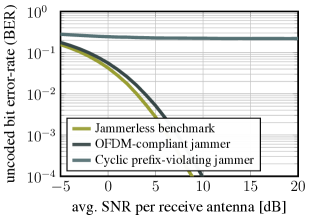
Figure 1: Bit error rates (BERs) of a jammerless system, a system attacked by an OFDM-compliant jammer, and a system attacked by a cyclic prefix-violating jammer. The latter two use a rank $B-1$ orthogonal projection for mitigating the jammer.

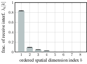
Figure 2: Histogram of the fraction of receive interference over the different spatial dimensions (sorted in descending order of power). The receive interference occupies $L=4$ different dimensions. Error bars cover two standard deviations per side.

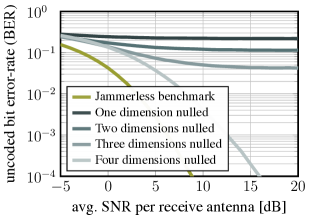
Figure 3: Bit error rate (BER) of a system that is attacked by a cyclic prefix-violating jammer. The system uses projections that null different numbers of dimensions (from one to four) of the receive interference for jammer mitigation.

IV-C Spatial Distribution of the Receive Interference

That the receive interference of a cyclic prefix-violating jammer occupies an $(L=4)$-dimensional subspace is further confirmed by fig:distribution, which shows a normalized histogram of the ordered singular values of the receive interference (measured across a coherence interval). That is, we denote the receive interference on the $k$th subcarrier over a coherence interval by $\hat{{\mathbf{Y}}}_{R}[k]\in\mathbb{C}^{B\times M}$ (which consists of $M$ receive vectors) and decompose it using a singular-value decomposition as $\hat{{\mathbf{Y}}}_{R}[k]=\mathbf{U}[k]\mathbf{\Sigma}[k]\mathbf{V}^{H}[k]$, where the diagonal elements $\sigma_{b}[k]$ of $\mathbf{\Sigma}[k]$ are sorted in descending order. Then we define the fraction of receive interference on the $b$th ordered spatial dimension as $\lambda_{b}[k]=\sigma_{b}[k]/\text{tr}(\mathbf{\Sigma}[k])$ for $b=1,\dots,B$. fig:distribution shows the mean (plus/minus two standard deviations) of the distribution over these $\lambda_{b}[k]$ (over all subcarriers $k$ and Monte-Carlo realizations). We see that while a single dimension contains a large part of the receive interference, it does not contain all of it. As predicted by thm:main, the receive interference occupies exactly $L=4$ spatial dimensions.

IV-D Nulling Different Numbers of Interference Dimensions

fig:projectors shows the performance when a communication system tries to mitigate a cyclic prefix-violating jammer by nulling different numbers of dimensions (from one to $L=4$) of the receive interference using an orthogonal projection before detecting the data using a ZF detector. In each case, the nulled dimensions are those where the receive interference is strongest. fig:projectors shows that the performance increases with each nulled dimension, as the residual jammer interference decreases until, with four nulled dimensions, the interference is removed completely. However, comparing the performance of this case against the performance of nulling a single dimension in the case of an OFDM-compliant jammer (fig:comp_noncomp) shows a performance loss of more than $5$ dB at a BER of $0.1\%$ (cf. also the large loss compared to the jammerless benchmark). This loss comes from the fact that removing the cyclic prefix violating jammer comes at the cost of $L=4$ degrees of freedom whereas nulling an OFDM-compliant jammer only costs one degree of freedom (out of a total of $B=8$ degrees of freedom). These results show that, if the jammer’s delay spread $L$ is large, jammer mitigation through linear spatial filtering becomes less effective—if $L$ approaches $B$, it becomes completely infeasible.

V The Way Forward: Some (Im)Possibilities

This letter has revealed a difficulty of MIMO jammer mitigation in OFDM. We remark that this difficulty is not simply an artifact of OFDM, but is in fact inherent to jammers with frequency-selective channels. Mitigating such a jammer using orthogonal projections in the time-domain would also require nulling of $L$ dimensions (for a single-antenna jammer)—every dimension corresponding to a tap of the jammer’s channel impulse response—at the cost of $L$ degrees of freedom. For this reason, one possible way forward for communication systems that pursue jammer resilience based on MIMO processing seems to avoid frequency-selective channels altogether. This means that communication has to be restricted to narrowband channels, either at the cost of achievable data rates, or by using multiple narrowband carriers in parallel [16, Sec. 12.1].

What this letter has conclusively established is that the common approach of modeling single-antenna jammers with frequency-selective channels in OFDM as frequency-flat single-antenna jammers is inaccurate, and that the actual high-rank interference reduces the effectiveness of linear spatial filtering.

References

- [1] H. Pirayesh and H. Zeng, “Jamming attacks and anti-jamming strategies in wireless networks: A comprehensive survey,” IEEE Commun. Surveys Tuts., vol. 9, no. 2, pp. 767–809, 2022.
- [2] Y. Léost, M. Abdi, R. Richter, and M. Jeschke, “Interference rejection combining in LTE networks,” Bell Labs Tech. J., vol. 17, no. 1, pp. 25–50, Jun. 2012.
- [3] G. Marti, T. Kölle, and C. Studer, “Mitigating smart jammers in multi-user MIMO,” IEEE Trans. Signal Process., vol. 71, pp. 756–771, 2023.
- [4] T. Hwang, C. Yang, G. Wu, S. Li, and G. Y. Li, “OFDM and its wireless applications: a survey,” IEEE Trans. Veh. Technol., vol. 58, no. 4, pp. 1673–1694, May 2008.
- [5] T. T. Do, E. Björnsson, E. G. Larsson, and S. M. Razavizadeh, “Jamming-resistant receivers for the massive MIMO uplink,” IEEE Trans. Inf. Forensics Security, vol. 13, no. 1, pp. 210–223, Jan. 2018.
- [6] H. Akhlaghpasand, E. Björnsson, and S. M. Razavizadeh, “Jamming suppression in massive MIMO systems,” IEEE Trans. Circuits Syst. II, vol. 68, no. 1, pp. 182–186, Jan. 2020.
- [7] G. Marti, O. Castañeda, and C. Studer, “Jammer mitigation via beam-slicing for low-resolution mmWave massive MU-MIMO,” IEEE Open J. Circuits Syst., vol. 2, pp. 820–832, Dec. 2021.
- [8] S. Sodagari and T. C. Clancy, “Efficient jamming attacks on MIMO channels,” in IEEE Int. Conf. Commun. (ICC), Jun. 2012, pp. 852–856.
- [9] M. C. Mah, H. S. Lim, and A. W. C. Tan, “Improved channel estimation for MIMO interference cancellation,” IEEE Commun. Lett., vol. 19, no. 8, pp. 1355–1357, Aug. 2015.
- [10] Q. Yan, H. Zeng, T. Jiang, M. Li, W. Lou, and Y. T. Hou, “Jamming resilient communication using MIMO interference cancellation,” IEEE Trans. Inf. Forensics Security, vol. 11, no. 7, pp. 1486–1499, Jul. 2016.
- [11] H. Zeng, C. Cao, H. Li, and Q. Yan, “Enabling jamming-resistant communications in wireless MIMO networks,” in Proc. IEEE Conf. Commun. Netw. Security (CNS), Oct. 2017, pp. 1–9.
- [12] H. Pirayesh, P. K. Sangdeh, S. Zhang, Q. Yan, and H. Zeng, “JammingBird: Jamming-resilient communications for vehicular ad hoc networks,” in Proc. IEEE Int. Conf. Sensing, Commun., Netw., Jul. 2021, pp. 1–9.
- [13] S. Gollakota, F. Adib, D. Katabi, and S. Seshan, “Clearing the RF smog: making 802.11n robust to cross-technology interference,” in ACM SIGCOMM Comput. Commun. Rev., Aug. 2011, pp. 170–181.
- [14] C. Shahriar, M. La Pan, M. Lichtman, T. C. Clancy, R. McGwier, R. Tandon, S. Sodagari, and J. H. Reed, “PHY-layer resiliency in OFDM communications: a tutorial,” IEEE Commun. Surveys Tuts., vol. 17, no. 1, pp. 292–314, 2014.
- [15] I. Javed, A. Loan, and W. Mahmood, “Novel schemes for interference-resilient OFDM wireless communication,” Int. J. Commun. Syst., vol. 30, Dec. 2017, e3095.
- [16] A. Goldsmith, Wireless Communications. Cambridge Univ. Press, 2005.