Beginner’s guide to Aggregation-Diffusion Equations

Abstract

The aim of this survey is to serve as an introduction to the different techniques available in the broad field of Aggregation-Diffusion Equations. We aim to provide historical context, key literature, and main ideas in the field. We start by discussing the modelling and famous particular cases: Heat equation, Fokker-Plank, Porous medium, Keller-Segel, Chapman-Rubinstein-Schatzman, Newtonian vortex, Caffarelli-Vázquez, McKean-Vlasov, Kuramoto, and one-layer neural networks. In Section 4 we present the well-posedness frameworks given as PDEs in Sobolev spaces, and gradient-flow in Wasserstein. Then we discuss the asymptotic behaviour in time, for which we need to understand minimisers of a free energy. We then present some numerical methods which have been developed. We conclude the paper mentioning some related problems.

Reply to the referees.
Comments in blue are replies to the referee.
Comments in purple are additions suggested by other colleagues since the publication of the preprint

1 Introduction

The aim of this survey is to serve as a general introduction to the many models and techniques used to study the Aggregation-Diffusion family of equations

$$\frac{\partial\rho}{\partial t}=\operatorname{div}\Big{(}\rho\nabla(U^{\prime}(\rho)+V+W*\rho)\Big{)}.$$ (ADE)

This survey does not intend to provide an encyclopedic presentation including all possible references and results in maximal generality (this would be impossible), but to give newcomers a general overview of the subject.

2 Modelling

Let us discuss first the modelling, and then we devote Section 3 to several modelling problems which belong to this family. On the one hand, diffusion is usually modelled as a conservation law.

2.1 Continuity equations

Let $\rho$ be a density and $\omega\subset{\mathbb{R}^{d}}$ any control volume, if $\mathbf{F}$ is the out-going flux

$$\frac{\mathop{}\!\mathrm{d}}{\mathop{}\!\mathrm{d}t}\int_{\omega}\rho\mathop{}\!\mathrm{d}x=-\int_{\partial\omega}\mathbf{F}\cdot\mathbf{n}\mathop{}\!\mathrm{d}S=-\int_{\omega}\operatorname{div}\mathbf{F}\mathop{}\!\mathrm{d}x$$ (2.1)

Hence we arrive at the continuity equation

$$\frac{\partial\rho}{\partial t}=-\operatorname{div}\mathbf{F}.$$ (2.2)

For the transport of heat, we use Fourier’s law to model the flux $\mathbf{F}=-D\nabla\rho$ and yields the heat equation

$$\frac{\partial\rho}{\partial t}=D\Delta\rho.$$ (HE)

A generalisation of this problem which is used to the flow a gas through porous media. We derive the model as mass balance by writing the flux in terms of a velocity $\mathbf{v}$, i.e., $\mathbf{F}=-\rho\mathbf{v}$; we use Darcy’s law to relate the velocity with the pressure $p$ as $\mathbf{v}=-\frac{k}{\mu}\nabla p$; and lastly we use a general state equation $p=\phi(\rho)$, where for perfect gases $\phi(\rho)=p_{0}\rho^{\gamma}$. Eventually, we recover that $\mathbf{F}=-\nabla\Phi(\rho)$ for some non-decreasing $\Phi:\mathbb{R}\to\mathbb{R}$, and this yields the so-called Porous Medium Equation

$$\frac{\partial\rho}{\partial t}=\Delta\Phi(\rho).$$ (PME_Φ)

It is common to select $\Phi(\rho)=\rho^{m}$ for $m>0$. The most complete reference for this equation is [Váz06c]. Notice $\Delta\Phi(\rho)=\operatorname{div}(\Phi^{\prime}(\rho)\nabla\rho)$ so we take

$$U^{\prime\prime}(\rho)=\frac{\Phi^{\prime}(\rho)}{\rho}.$$ (2.3)

The classical modelling also allows for a transport velocity field $\mathbf{v}(t,x)$ to be included. For example, if a pollutant is being transported by water, then $\mathbf{v}(t,x)$ is the velocity of the water. The flux of mass being moved is recovered from the density and the velocity as $\rho\mathbf{v}$. A general flux then looks like

$$\mathbf{F}=-\nabla\Phi(\rho)+\rho\mathbf{v}.$$

Remark 2.1.

We do not discuss the case of sign-changing solutions. In that setting $u^{m}$ must be replaced by $|u|^{m-1}u$.

2.2 Particle systems

We can also understand transport from the particle perspective. Consider a known velocity field $\mathbf{v}(t,x)$. Consider $N$ particles with positions $X_{i}(t)$ of equal masses $1/N$ moving in the velocity field

$$\frac{\mathop{}\!\mathrm{d}X_{i}}{\mathop{}\!\mathrm{d}t}=\mathbf{v}(t,X_{i}(t)),\qquad i=1,\cdots,N.$$

Notice that the evolution of the particles is decoupled. To recover a PDE we consider the so-called empirical distribution defined as

$$\mu_{t}^{N}=\sum_{j=1}^{N}\frac{1}{N}\delta_{X_{j}(t)},$$ (2.4)

where $\delta_{x}$ is the Dirac delta at a point $x$. First, notice that

$$\frac{\mathop{}\!\mathrm{d}}{\mathop{}\!\mathrm{d}t}\int_{\mathbb{R}^{d}}\varphi(t,x)\mathop{}\!\mathrm{d}\mu^{N}_{t}(x) =\frac{\mathop{}\!\mathrm{d}}{\mathop{}\!\mathrm{d}t}\frac{1}{N}\sum_{j}\varphi(t,X_{j}(t))$$

$$=\frac{1}{N}\sum_{j}\left(\frac{\partial\varphi}{\partial t}(t,X_{j}(t))+\nabla\varphi(t,X_{j}(t))\cdot\frac{\mathop{}\!\mathrm{d}X_{j}}{\mathop{}\!\mathrm{d}t}\right)$$

$$=\frac{1}{N}\sum_{j}\left(\frac{\partial\varphi}{\partial t}(t,X_{j}(t))+\nabla\varphi(t,X_{j}(t))\cdot\mathbf{v}(t,X_{j}(t))\right)$$

$$=\int_{\mathbb{R}^{d}}\left(\frac{\partial\varphi}{\partial t}(t,x)+\nabla\varphi(t,x)\cdot\mathbf{v}(t,x)\right)\mathop{}\!\mathrm{d}\mu^{N}_{t}(x)$$

If $\varphi\in C^{1}_{c}((0,\infty)\times{\mathbb{R}^{d}})$ (i.e., $\varphi(0,x)=0$ and for $T$ large enough $\varphi(t,x)=0$ for $t\geq T$) we integrate in time to recover

$$\int_{0}^{\infty}\int_{\mathbb{R}^{d}}\Big{(}\frac{\partial\varphi}{\partial t}+\mathbf{v}\cdot\nabla\varphi\Big{)}\mathop{}\!\mathrm{d}\mu^{N}_{t}\mathop{}\!\mathrm{d}t=0.$$

Integrating by parts, we observe that this is the distributional formulation of the continuity equation

$$\partial_{t}\mu^{N}+\operatorname{div}(\mu^{N}\mathbf{v})=0.$$

Aggregation and Confinement can be modelled by considering interacting particles where the velocity field is aware of other particles

$$\frac{\mathop{}\!\mathrm{d}X_{i}}{\mathop{}\!\mathrm{d}t}=-\sum_{\begin{subarray}{c}j=1\\ j\neq i\end{subarray}}^{N}\frac{1}{N}\nabla W(X_{i}-X_{j})-\nabla V(X_{i}),\qquad i=1,\cdots,N.$$

The first term models the interactions between particles, with attract/repel each other as a function of their relative position, and the second term models a field attracting/repelling every particle. Noticing that

$$\sum_{\begin{subarray}{c}j=1\\ j\neq i\end{subarray}}^{N}\frac{1}{N}\nabla W(x-X_{j}(t))=\int_{\mathbb{R}^{d}}\nabla W(x-y)\mathop{}\!\mathrm{d}\mu^{N}_{t}(y)$$

we deduce from the previous reasoning that the empirical measure $\mu^{N}$ is a distributional solution of the Aggregation-Confinement Equation

$$\partial_{t}\mu=\operatorname{div}(\mu\nabla(W*\mu+V)).$$ (2.5)

Linear diffusion can be added to the particle system by introducing noise and working with Stochastic ODEs and a mean-field approximation (see Section 3.8).

As we will see below, special attention has been paid to the case $V=0$ which is simply called Aggregation Equation

$$\frac{\partial\rho}{\partial t}=\operatorname{div}(\rho\nabla W*\rho).$$ (AE)

As a toy model we will also discuss the confinement problem

$$\frac{\partial\rho}{\partial t}=\operatorname{div}(\rho\nabla V).$$ (CE)

Joining the many-particle approximation for aggregation with the Porous Medium diffusion we recover (ADE). If we look for solutions defined in the whole space, then it is natural to consider only the case of finite mass. Hence, we assume $\rho\in L^{1}({\mathbb{R}^{d}})$ and, in some sense,

$$\rho_{t}(x)\to 0\text{ as }|x|\to\infty.\\$$ (2.6)

2.3 Boundary conditions in bounded domains of ${\mathbb{R}^{d}}$

The problems above are often posed in the whole space ${\mathbb{R}^{d}}$. However, sometimes it is convenient to restrict them to bound domains, specially for the numerical analysis. Here and below we will denote by $\Omega$ an open and bounded set of ${\mathbb{R}^{d}}$ with a smooth boundary. Although it is possible to study these kinds of problems in less smooth domain (Lipschitz boundary, interior point conditions, etc…) this introduces additional difficulties we will not discuss. Since with this kind of equation we intend to model systems that conserve mass, there are two natural approaches.

2.3.1 No-flux conditions

We can stablish that no mass will cross the boundary of $\Omega$, $\partial\Omega$. Going back to (2.1), a natural way is to establish no-flux conditions $\mathbf{F}\cdot\mathbf{n}=0$ on $\partial\Omega$. With our choice of flux this means

$$\rho\nabla(U^{\prime}(\rho)+V+W*\rho)\cdot\mathbf{n}=0\qquad\text{ for }t>0\text{ and }x\in\partial\Omega$$ (BC)

where again $\rho_{0}$ is known, and we have to be a little careful with the notion of convolution when $\rho$ is only defined in $\Omega$. For this, we consider the extended notion

$$W*\rho\equiv W*\widetilde{\rho},\qquad\text{where }\widetilde{\rho}=\begin{dcases}\rho&\text{in }\Omega,\\ 0&\text{elsewhere}.\end{dcases}$$

In fact, the problem (ADE) with general $V$ and $W$ in a bounded domain is rather delicate in terms of a priori estimates (see Section 4.2.3). It is sometimes preferable to discuss the generalisation

$$\frac{\partial\rho}{\partial t}=\operatorname{div}\Big{(}\rho\nabla(U^{\prime}(\rho)+V+\mathcal{K}\rho)\Big{)},\qquad\text{where }\mathcal{K}\rho(x)=\int_{\Omega}K(x,y)\rho(y)\mathop{}\!\mathrm{d}y,$$ (ADE^∗)

and with the corresponding boundary conditions

$$\rho\nabla(U^{\prime}(\rho)+V+\mathcal{K}\rho)\cdot\mathbf{n}=0,\qquad\text{on }\partial\Omega.$$ (BC^∗)

If $\Omega$ is bounded we will choose

$$\nabla V\cdot\mathbf{n}=0\text{ in }\partial\Omega,\qquad\text{ and }\qquad K\in C_{c}(\Omega\times\Omega).$$ (2.7)

A very typical example is

$$K(x,y)=\eta(x)W(x-y)\eta(y)$$ (2.8)

with $\eta\in C^{\infty}_{c}(\Omega)$.

2.3.2 Periodic boundary conditions

Another approach is to stablish that any mass that crosses the boundary will “come back” on the opposite side. This happens, for example, if all data are periodic. Some papers have studied periodic solutions defined over the unit cube $[0,1]^{d}$ (or, equivalently, the torus $\mathbb{T}^{d}$). In $d=1$ this is equivalent to studying solutions defined over the unit circle $\mathbb{S}^{1}$. This is the case of the Kuramoto model described below. An example of the case $d=2$ can be found in [CGPS20a].

2.4 Free energy

We conclude this section by introducing a functional which will be very useful below. We will show how (ADE) is related to the free energy

$$\mathcal{F}(\rho)=\int_{\Omega}U(\rho)+\int_{\Omega}V\rho+\frac{1}{2}\iint_{\Omega\times\Omega}W(x-y)\rho(x)\rho(y)\mathop{}\!\mathrm{d}x\mathop{}\!\mathrm{d}y,$$ (FE)

whereas (ADE^∗) is related to the more general free energy

$$\mathcal{F}(\rho)=\int_{\Omega}U(\rho)+\int_{\Omega}V\rho+\frac{1}{2}\iint_{\Omega\times\Omega}K(x,y)\rho(x)\rho(y)\mathop{}\!\mathrm{d}x\mathop{}\!\mathrm{d}y.$$ (FE^∗)

For convenience, let us define the function

$$\frac{\delta\mathcal{F}}{\delta\rho}[\rho]\vcentcolon=U^{\prime}(\rho)+V+\int_{\Omega}K(\cdot,y)\rho(y)\mathop{}\!\mathrm{d}y.$$ (2.9)

This is called first variation of the free energy, and we will explain its importance below in Section 4.2.4. Hence, (ADE^∗) can be re-written as

$$\frac{\partial\rho}{\partial t}=\operatorname{div}\left(\rho\nabla\frac{\delta\mathcal{F}}{\delta\rho}\right)$$ (2.10)

for ${\mathcal{F}}$ given by (FE).

Occasionally, it will be convenient for us to use the free energies of each of the terms. Hence, we define

$$\mathcal{U}[\rho]=\int_{\mathbb{R}^{d}}U(\rho),\qquad\mathcal{V}[\rho]=\int_{\mathbb{R}^{d}}V\rho,\qquad\mathcal{W}[\rho]=\frac{1}{2}\iint_{\mathbb{R}^{d}}W(x-y)\rho(x)\rho(y)\mathop{}\!\mathrm{d}x\mathop{}\!\mathrm{d}y.$$ (2.11)

2.5 A comment on mass conservation

Our evolution problem need, of course, an initial state $\rho_{0}$. Throughout this survey we will usually restrict ourselves non-negative unit mass initial data, i.e.,

$$\int_{{\mathbb{R}^{d}}}\rho_{0}(x)=1.$$ (U₀)

All the equations presented above are of “conservation type”. This means we expect preservation of mass, i.e., that provided unit initial mass (U₀) then there will be non-negative unit initial mass for all times, i.e.,

$$\int_{\mathbb{R}^{d}}\rho_{t}=1,\qquad\forall t>0.$$ (U)

3 Famous particular cases

3.1 Heat equation and Fokker-Plank

As explained above, the heat equation (HE) is the most classical example in our family of equations. It corresponds to (ADE) with the choices $U=\rho\log\rho$ and $V=W=0$. In ${\mathbb{R}^{d}}$ It is well known that (HE) admits the Gaussian solution

$$K_{t}(x)=(4\pi t)^{-\frac{d}{2}}\exp\left(-\frac{|x|^{2}}{4t}\right).$$

All solutions (with suitable initial data) are precisely of the form

$$\rho_{t}=K_{t}*\rho_{0},$$

and it is not difficult to check that

$$\|\rho_{t}\|_{L^{1}}=M,\qquad\|\rho_{t}-MK_{t}\|_{L^{1}}\to 0\quad{as}t\to\infty.$$

A good survey on the matter can be found in [Váz17a].

The fundamental solution $K_{t}$ is of the so-called self-similar type

$$K_{t}(x)=A(t)F\left(\frac{x}{\sigma(t)}\right).$$ (SS)

In this expression, $F$ is usually called self-similar profile and $\sigma(t),A(t)$ the scaling parameters. Due to mass conservation the natural choice is $A(t)=\sigma(t)^{-d}$. Plugging (SS) into (HE) and setting the total mass $\int K_{t}=1$ yields the Gaussian. Since (HE) is linear, $MK_{t}$ is a solution of mass $M$. Usually, the self-similar solution has $\sigma(t)$ increasing, and it only makes sense to consider $\sigma(t)\geq 0$. Hence, we make the choice $\sigma(0)=0$ that corresponds to $K_{t}=\delta_{0}$, a Dirac delta at $0$. This type of solutions with $\rho_{0}=\delta_{0}$ are called source-type solutions.

This nice convolutional representation is not available in more general settings. There are several other ways to study the asymptotic behaviour. One of the key tricks is the study of the self-similar change of variable

$$\rho(x,t)=u(y,\tau)(1+t)^{-\frac{d}{2}},\qquad 2\tau=\log(1+t),\qquad y=(1+t)^{-\frac{1}{2}}x,$$

which leads to the so-called linear Fokker-Planck equation

$$\frac{\partial u}{\partial\tau}=\Delta_{y}u+\operatorname{div}(uy).$$ (HE-FP)

This equation corresponds to

$$U_{1}(\rho)=\rho\log\rho,$$

$V=\frac{|x|^{2}}{2}$ and $W=0$. Notice that stationary states can be obtained as solutions of the equation for the flux $\log u+\frac{|x|^{2}}{2}=-h$. This yields the Gaussian profile

$$\widehat{u}(y)=AG(y),\qquad G(y)=\frac{1}{\sqrt{2\pi}}e^{-\frac{|y|^{2}}{2}}.$$ (3.1)

The constant $A$ is the unique value such that $\int\rho_{t}=M$. In original variable, we recover $MK_{t}$.

3.2 Porous medium equation

As presented in the introduction, the most common example of (PME_Φ) is the Porous Medium Equation

$$\frac{\partial\rho}{\partial t}=\Delta\rho^{m}.$$ (PME)

The range $m\in(0,1)$ is sometimes called Fast Diffusion Equation. The (PME) corresponds, for $m\neq 1$, to

$$U_{m}(\rho)=\frac{\rho^{m}}{m-1}$$

and $V=W=0$. Notice that as $m\to 1$ we have $\rho^{m-1}/(m-1)$ tends to $\log\rho$ and hence $U_{m}$ tends to $U_{1}$. Notice that, due to the homogeneity of the equation, after rescaling space and time, we can preserve the equation (without introducing constants) and can work with (U₀).

Similarly to the heat equation, a suitable change of variable (detailed below in Section 5.1.1) converts (PME) into

$$\frac{\partial u}{\partial t}=\Delta u^{m}+\operatorname{div}(ux)$$ (PME-FP)

This corresponds to $U=U_{m}$ and $V=\frac{|x|^{2}}{2}$ and $W=0$. (PME-FP) admits a stationary solution given by the so-called Barenblatt profiles

$$\hat{u}(x)=F_{B}(x),\qquad F_{B}(x)\vcentcolon=\left(C-\tfrac{m-1}{2m}{|x|^{2}}\right)^{\frac{1}{m-1}}_{+},$$ (3.2)

where $C\geq 0$. For $m>1$ they have compact support, and for $m\in(0,1)$ they have power-like tails. To check whether finite-mass states are available we compute

$$\int_{\mathbb{R}^{d}}F_{B}\approx c+\int_{1}^{\infty}r^{\frac{2}{m-1}}r^{d-1}\mathop{}\!\mathrm{d}r.$$

Hence, finite mass steady states are only when $m>\frac{d-2}{d}$. This number is critical, as well will see below. Undoing the change of variables we arrive at the self-similar solution

$$B_{t}=t^{-\alpha}(C-k|x|^{2}t^{-2\beta})^{\frac{1}{m-1}}_{+},\qquad\text{where }\alpha=\tfrac{d}{d(m-1)+2},\,\beta=\tfrac{\alpha}{d},\,k=\tfrac{\alpha(m-1)}{d}.$$ (ZKB)

This solution is usually denoted ZKB after Zel’dovich and Kompaneets, and Barenblatt (see [Váz06c] and the references therein). Usually this is shortened to Barenblatt. When $m>\frac{d-2}{d}$ there is a unique constant $C$ so that (U). It can be explicitly computed (see [Váz06c, Section 17.5]).

As we let $m\searrow\frac{d-2}{d}$ we get $C\nearrow\infty$, so for $m=\frac{d-2}{d}$ we expect $B_{t}=\delta_{0}$. In fact, Brezis and Friedman [BF83a] showed that if $m\leq\frac{d-2}{d}$ and $\rho_{0}^{(j)}\in L^{1}({\mathbb{R}^{d}})$ are a sequence of initial data converging to $\delta_{0}$, then the corresponding solutions converge to $\rho^{(j)}(t,x)\to\delta_{0}(x)\otimes 1(t)$. Therefore, very fast diffusion cannot diffuse a $\delta_{0}$. This is because the diffusion coefficient is $m\rho^{m-1}$. For $m\ll 1$ this means that small values of $\rho$ are indeed diffused fast (hence the name of “fast diffusion”). However, in regions where $\rho$ is large the diffusion is slow.

It is also worth pointing to the equivalent formulation in the so-called pressure variable $u=U^{\prime}(\rho)$. We recover the Hamilton-Jacobi type equation

$$\frac{\partial u}{\partial t}=\Phi^{\prime}(\rho)\Delta u+|\nabla u|^{2},$$

where we recall the relation (2.3). Notice that $\Phi^{\prime}(\rho)$ can be written as a non-linear function of $u$. This formulation is convenient when $m>1$ since $u=\frac{m}{m-1}\rho^{m-1}$. This presentation is much better for the study of viscosity solutions (see [CV99a, BV05a]).

First results of asymptotic behaviour for $m>1$ were obtained by regularity, self-similarity, and comparison arguments in the late 70s and early 80s (see [FK80a] and the references therein). Self-similar analysis and relative entropy arguments were later developed to improve the theoretical understanding (see Sections 5.1.1 and 5.2.3). For a detailed explanation of the theory see [Váz06b, Váz06c].

Remark 3.1.

(HE) and (PME) are “diffusive”. This can be seen in different directions. For example, at a point $(t_{0},x_{0})$ of local maximum of $\rho$ we get $\Delta\rho^{m}\leq 0$ and hence $\frac{\partial\rho}{\partial t}\leq 0$, i.e., the maximum values decays. This is strongly related to the maximum principle. The converse happens to the minimum if it exists (notice that non-negative solutions in ${\mathbb{R}^{d}}$ will tend to $0$ as $|x|\to\infty$).

Remark 3.2.

Let us recall some “numerological values”. The value $m=1-\frac{2}{d}$ is the critical value for finite-mass Barenblatt. It is also be the critical value below which there is finite-time extinction (see Section 4.2.1). The (3.2) has finite $\lambda$-moment, i.e.,

$$\int_{\mathbb{R}^{d}}|x|^{\lambda}B_{t}(x)\mathop{}\!\mathrm{d}x<\infty$$

if and only if $m>1-\frac{2}{d+\lambda}$. In Section 4.3.4 we will present a third relevant value $m=1-\frac{1}{d}$ coming from the Wasserstein gradient-flow analysis.

Remark 3.3.

We will not discuss here the limit $m\to 0$. In this direction there are two possibilities. On the one hand, some authors have discussed the rescaled limit $\frac{u^{m}}{m}\to\log u$, and we arrive at the logarithmic diffusion equation $\partial_{t}u=\Delta\log(u)$. We point to [Váz06b, Section 8.2] for a discussing on this topic and [Váz06b, Section 8.4] for historical notes. On the other hand, some authors choose to look at the limit $|u|^{m-1}u\to\operatorname{sign}(u)$ leads to the so-called Sign Fast Diffusion Equation $\partial_{t}u=\Delta\operatorname{sign}(u)$. Some results in this direction are available [BF12a].

3.3 Transport problem with known potential

To understand the transport terms in the (ADE) family, we will discuss the toy problem

$$\frac{\partial\rho}{\partial t}=\operatorname{div}(\rho\nabla V)$$

where $V$ is known and does not depend on $t$. Imagine that $\rho_{0}\geq 0$ is radially symmetric function. Computing the balance of mass of a ball $B_{r}$ we get

$$\frac{\mathop{}\!\mathrm{d}}{\mathop{}\!\mathrm{d}t}\int_{B_{r}}\rho_{t}=\int_{B_{r}}\operatorname{div}(\rho\nabla V)=\int_{\partial B_{r}}\rho\nabla V\cdot x.$$ (3.3)

If $\nabla V\cdot x\leq 0$ all balls $B_{r}$ are “loosing mass”, i.e., then mass if always flowing “away” from $0$ and towards infinity. Hence, we can think of these kinds of potentials as “diffusive” (but not as strongly as in the sense of Remark 3.1). We will show below by explicitly solving these problems that potentials such that $\nabla V\cdot x\geq 0$ will attract mass towards $0$, asymptotically (or even instantaneously) creating a singularity.

3.4 Keller-Segel model

The Keller-Segel [KS70a] (or Patlak-Keller-Segel model [Pat53a]) model for describes the motion of cells by chemotactical attraction by means of the coupled system

$$\begin{dcases}\frac{\partial\rho}{\partial t}=\Delta\rho-\operatorname{div}(\rho\nabla V_{t})\\ -\Delta V_{t}=\rho_{t}.\end{dcases}$$ (KSE)

This model was first studied for $d=2$. Some authors replace the second equation by a more general evolutionary problem $\varepsilon\frac{\partial V_{t}}{\partial t}-\Delta V_{t}+\alpha V_{t}=\rho_{t}$. We will discuss (KSE), which can be thought as the limit $\varepsilon,\alpha\to 0$. This simplification was first introduced by [Nan73a] to model the case where the diffusion of the chemical is much faster than its production.

So far, this model is not in the (ADE) family. However, the can analysis the equation for $V_{t}$ to recover some information. In ${\mathbb{R}^{d}}$ we can use the Fourier transform $\mathrm{F}$ for the elliptic problem to recover

$$|\xi|^{2}\mathrm{F}[V_{t}](\xi)=\mathrm{F}[\rho_{t}]$$

and hence we can solve and recover $V_{t}=W_{\rm N}*\rho$, where $W_{\mathrm{N}}=\mathrm{F}^{-1}[|\xi|^{-2}]$. In fact, we have the closed expression

$$W_{\mathrm{N}}(x)=\begin{dcases}-\frac{1}{2\pi}\log|x|&\text{if }d=2,\\ \frac{1}{d(d-2)\omega_{d}}|x|^{2-d}&\text{if }d>2.\end{dcases}$$ (3.4)

Notice that $-\Delta W_{\rm N}=\delta_{0}$. The so-called Newtonian potential corresponds to $\rm N=-W_{\rm N}$. Eventually, we can write this problem as (ADE) where $U=\rho\log\rho$, $V=0$ and $W=-W_{\rm N}$.

We can think about the convolution term $W*\rho_{t}$ as an aggregation potential. The justification is the following. If $\rho_{t}$ is non-increasing, then $V_{t}=W*\rho_{t}$ is also non-increasing, and hence $\nabla V_{t}\cdot x\leq 0$. Going back to Section 3.3, this is what we called aggregation potentials. Unfortunately, we do not have in general the sign $\nabla V_{t}\cdot x\leq 0$ for all $t,x>0$. In fact, (KSE) does not “prefer” $x=0$ from other points.

Changing the sign of the aggregation to $\frac{\partial\rho}{\partial t}=\Delta\rho+\operatorname{div}(\rho\nabla V_{t})$ makes the problem more regularising. In [Bil92a] the author proves global well-posedness of that problem for $d=3$ in a bounded domain with no-flux condition was shown to have.

Sometimes it is convenient to express the problem in a single equation using operator notation:

$$\frac{\partial\rho}{\partial t}=\Delta\rho-\operatorname{div}(\rho\nabla(-\Delta)^{-1}\rho).$$

When written in this form, the authors usually allow for any initial mass $\|\rho_{0}\|_{L^{1}}$. We can rescale to impose (U₀). If we let $\chi=\|\rho_{0}\|_{L^{1}}$ and $u(t,x)=\rho(t,x)/\chi$ we arrive at the equation

$$\frac{\partial u}{\partial t}=\Delta u-\chi\operatorname{div}(u\nabla(-\Delta)^{-1}u).$$ (KSE_χ)

In bounded domains some authors introduce Neumann boundary conditions $\frac{\partial u}{\partial n}=\frac{\partial V}{\partial n}=0$. The authors of [JL92a] extend the problem to $-\Delta V=\beta u-\mu$ which a few authors later called Jäger-Luckhaus problem (e.g., [Sen05a]). This is equivalent to replacing $(-\Delta)^{-1}$ by $(-\Delta+\rm{id})^{-1}$.

Some authors later introduced the Keller-Segel model with Porous Medium Diffusion. One of the model arguments is that $m>1$ would deal with “over-crowding” (i.e., the formation of Dirac deltas). We arrive at the problem

$$\frac{\partial\rho}{\partial t}=\Delta\rho^{m}-\chi\operatorname{div}(\rho\nabla(-\Delta)^{-1}\rho).$$ (KSE_m,χ)

This model has the advantage of not having finite time blow-up (see [CC06a]). Existence and uniqueness of solutions for $m>1$ and a family of $W$ covering $W_{\rm N}$ can be found in [BRB11a]. Some authors replace $(-\Delta)^{-1}$ by $(-\Delta+\gamma\rm{id})^{-1}$, see, e.g., [LS07a, SK06a, Sug07b, Sug07c].

As we will discuss below, (KSE_m,χ) admits global solutions in the sub-critical range $m>2-\frac{2}{d}$. However, for $m<2-\frac{2}{d}$ there is finite-time blow-up. In the critical case blow-up depends on $\chi$. Curiously enough, the first case studied was $d=2$ and $m=1$, which is critical. A good explanation of this dichotomy is the free-energy minimisation argument which we will provide in Section 6.3.

3.5 Chapman-Rubinstein-Schatzman

In the context of superconductivity [CRS96a] introduced a mean-field model for “the motion of rectilinear vortices in the mixed state of a type-II semiconductor”. They argue this is the limit where the Ginzburg-Landau parameter $\kappa$ tends to $+\infty$ and the number of vortices becomes large one recovers the problem

$$\begin{dcases}\frac{\partial\rho}{\partial t}=\operatorname{div}(|\rho|\nabla V_{t})\\ -\Delta V_{t}+V_{t}=\rho_{t}.\end{dcases}$$ (CRSE)

The model was first introduced in $\mathbb{R}^{2}$. Then, the authors also make a particularisation to a bounded domain $\Omega$ where they introduce Dirichlet conditions for $V_{t}(x)=h_{0}$ on $\partial\Omega$, and flux conditions setting the number of vortices crossing the boundary $|\rho|\nabla v\cdot n$ known.

In fact, when $\rho\geq 0$ it becomes of our class (ADE) (or (ADE^∗) in bounded domains). On ${\mathbb{R}^{d}}$ we can solve as before to recover $V_{t}=W*\rho_{t}$ where $W=\mathrm{F^{-1}}[(1+|\xi|^{2})^{-1}]$. As long as $\rho\geq 0$, this model corresponds to (ADE) where $U,V=0$. If we work in a bounded domain $\Omega$ the homogeneous Dirichlet condition we recover (ADE^∗) where $U,V=0$ and $K$ is the Green kernel of the equation. Notice that $K$ is not a compactly supported in $\Omega\times\Omega$.

There is extensive literature on this problem. First, there were different works applying PDE theory. First, [CRS96a] proved existence of the problem posed in bounded domains. Then in [HS98a] the authors work with non-negative $\rho_{0}$ and compactly supported, using generalised characteristics. We also point to [SS99a] where the authors perform a vanishing viscosity analysis in bounded domains.

Later, some authors applied Optimal Transport methods, in particular the 2-Wasserstein gradient-flow approach. In [AS08a] the authors worked in with non-negative probability measures in a bounded domain, i.e., $\mathcal{P}_{2}(\overline{\Omega})$. Later, the work was extended in [AMS11a] to a bounded domain and signed measures. They extend the Wasserstein distance to signed measures and in fact they minimise a localised energy in the space of signed unit measures in ${\mathbb{R}^{d}}$ to recover a problem of the form

$$\frac{\partial\rho}{\partial t}=\operatorname{div}(\mathbf{1}_{\Omega}|\rho|\nabla V_{t}),\qquad\text{for }t>0,x\in{\mathbb{R}^{d}}.$$

This sparked broader interest in the family of aggregation equations (AE).

3.6 Newtonian vortex problem

In [LZ99a] the authors justify that a different limit from Gizburg-Landau equations leads to the problem without zero-order term

$$\begin{dcases}\frac{\partial\rho}{\partial t}=\operatorname{div}(\rho\nabla V_{t})\\ -\Delta V_{t}=\rho.\end{dcases}$$ (NVE)

Again, this can be set in ${\mathbb{R}^{d}}$ or in a bounded domain (with suitable boundary conditions).

This problem also attracted several authors, who brought different approaches. [LZ99a] the authors construct solutions by characteristics with the so-called “vortex-blob” method. In [MZ05a] the authors prove existence of renormalised solutions. The authors of [BLL12a] study positive and negative solutions. This is equivalent to studying non-negative solutions of the problems

$$\frac{\partial\rho}{\partial t}=\pm\operatorname{div}(\rho\nabla W_{\rm N}*\rho).$$

The $W=-W_{\rm N}$ can also be seen of the problem $W=W_{\rm N}$ but taken backwards in time. In fact, the authors prove that the $+$ sign leads to asymptotic dispersion whereas $-$ leads to blow-up.

3.7 The Caffarelli-Vázquez problem

In [CV11b], Caffarelli and Vázquez introduced a non-local porous medium-type equation given by

$$\begin{dcases}\frac{\partial\rho}{\partial t}=\operatorname{div}(\rho\nabla V_{t})\\ (-\Delta)^{s}V_{t}=\rho,\end{dcases}$$

where $(-\Delta)^{s}$ denotes the fractional Laplacian. In ${\mathbb{R}^{d}}$ this operator is to the operational fractional power of the Laplacian, which can be rigorously defined as the operator with Fourier symbol $|\xi|^{2s}$. This problem is often called Caffarelli-Vázquez problem and is often written in the compact form

$$\frac{\partial\rho}{\partial t}=\operatorname{div}(\rho\nabla(-\Delta)^{-s}\rho).$$ (CVE)

This is a “diffusive” operator. To solve the fractional Laplace equation we take $W=\mathrm{F}^{-1}[|\xi|^{-2s}]$, and we recover the so-called Riesz potential

$$W_{\rm R}(x)=c_{d,s}\begin{dcases}|x|^{2s-d}&\text{if }2s<d,\\ \log|x|&\text{if }2s=d\end{dcases}$$

The properties convolution properties of the Riesz potential where already well known in Harmonic Analysis. There has been a lot of analysis for this equation: asymptotic analysis [CV11c], sign-changing case and self-similar solutions [BIK15a], regularity theory [CSV13a, CV15a], and in [SV14a] that the limit as $s\to 1$ is (NVE). In [LMS18a] the authors construct a solution through the Wasserstein gradient-flow theory described in Section 4.3.

3.8 McKean-Vlasov and Kuramoto problems

The McKean-Vlasov process is given by the stochastic differential equation

$$\mathop{}\!\mathrm{d}X_{t}=a_{t}\mathop{}\!\mathrm{d}\mathcal{B}_{t}+b_{t}\mathop{}\!\mathrm{d}t$$

where $a_{t},b_{t}$ may depend on $X_{t}$ and its law, and $\mathcal{B}_{t}$ is a Wiener process, i.e., we introduce Brownian motion. We can extend this idea to a system of $N$ particles driven by coupled McKean-Vlasov equations. If we consider that $a_{t}$ is constant, say $a_{t}=\sqrt{2\beta^{-1}}$, and $b_{t}$ is given by the interaction we can arrive at

$$\mathop{}\!\mathrm{d}X_{t}^{(i)}=-V(X_{t}^{(i)})-\frac{1}{N}\sum_{\begin{subarray}{c}j=1\\ j\neq i\end{subarray}}^{N}\nabla W(X_{t}^{(i)}-X_{t}^{(j)})\mathop{}\!\mathrm{d}t+\sqrt{2\beta^{-1}}\mathop{}\!\mathrm{d}\mathcal{B}_{t}.$$

Through arguments of mean-field theory (or propagation of chaos see, e.g., [JW17a]), one arrives asymptotically as $N\to\infty$ to (ADE) with linear diffusion $U=\beta\rho\log\rho$ (see, e.g., [CGPS20a]). This is the reason the problem

$$\frac{\partial\rho}{\partial t}=\beta^{-1}\Delta\rho+\operatorname{div}(\rho\nabla(V+W*\rho))$$ (McKVE)

is sometimes called McKean-Vlasov problem (see, e.g., [CGPS20a]). However, this denotation is not universal (see, e.g., [CGYZ23a]).

Y. Kuramoto [Kur75a] introduced a model for synchronisation of chemical and biological oscillators, and it has been well-received by the community in neuroscience. It is a particular case of McKean-Vlasov problem in $d=1$ where $X_{t}^{(i)}$ models the phase of a coupled oscillator. Therefore, we take $X_{t}^{(i)}\in[0,2\pi)$ or, equivalently, periodic boundary condition. The particular choices are $V(x)=-\omega_{i}$ the natural frequency of the system, and $W(x)=\sin(x)$. The resulting (ADE) is known as the Kuramoto model

$$\begin{dcases}\frac{\partial\rho}{\partial t}=\beta^{-1}\Delta\rho+\operatorname{div}(\rho(-\omega+\sin*\rho))&t>0,x\in(0,2\pi),\\ \rho_{t}\text{ is }2\pi-\text{periodic}.\end{dcases}$$ (KE)

The case $\beta^{-1}=0$ is also interesting. An interesting analysis of this problem without diffusion (i.e., $\beta^{-1}=0$) can be found in [CCHKK14a].

3.9 The neural networks of machine learning

A neural network is no more than a specific type of parametric function accepting an input vector $x\in{\mathbb{R}^{d}}$ and returning $y\in\mathbb{R}$. If the output is higher dimensional, then we can create a neural network for each output. In this context “training” corresponds to optimising the parameters to fit a set of prescribed data (supervised learning) or to achieve some objective (unsupervised learning). Neural networks are form by connecting so-called perceptron. A perceptron is a parametric function of the form

$$x\longmapsto\sigma(\theta_{1}\cdot x+\theta_{2})$$

where $\sigma$ is called the activation function and $\theta_{1}\in{\mathbb{R}^{d}},\theta_{2}\in\mathbb{R}$. A one-layer neural network is the linear combination of the output of $N$ perceptrons, and can be expressed

$$f_{N}(x|w,\theta)\vcentcolon=\sum_{i=1}^{N}\frac{w_{i}}{N}\sigma(\theta_{1,i}\cdot x+\theta_{2,i})$$

where $w_{i}\in\mathbb{R}$, $\theta_{1,i}\in{\mathbb{R}^{d}}$, and $\theta_{2,i}\in\mathbb{R}$. The aim is, for $N$ fixed, to find the best parameter to approximate a target function $f$, in the sense that

$$\min_{(w,\theta)}\int_{\mathbb{R}^{d}}|f(x)-f_{N}(x|w,\theta)|^{2}\mathop{}\!\mathrm{d}x.$$ (3.5)

The quadratic error can be replaced by more general functions.

In [FF22a] the authors give a nice presentation of the following continuous formulation, i.e., limit as $N\to\infty$. When can let $\xi_{i}\vcentcolon=(w_{i},\theta_{1,i},\theta_{2,i})$, $\Xi(\xi,x)\vcentcolon=w\sigma(\theta_{1,i}x+\theta_{2,i})$, and define the empirical distribution

$$\mu_{N}\vcentcolon=\frac{1}{N}\sum_{i=1}\delta_{\xi_{i}}.$$ (3.6)

For convenience, define $\Omega$ as the set of admissible $\xi$. Then, the value of the neural network can be computed as

$$f_{N}(x|w,\theta)=\int_{\Omega}\Xi(\xi,x)\mathop{}\!\mathrm{d}\mu_{N}(\xi).$$

We can rewrite the (3.5) to a minimisation problem over the set of empirical distributions given by (3.6). The limit as $N\to\infty$ is now clear, we pass to the minimisation problem over $\mathcal{P}(\Omega)$. To smoothen the problem the authors allow for a penalisation $\widehat{V}$ (of type $|\xi|^{2}/2$), which can be understood as trying to prevent overfitting. We land on the problem

$$\min_{\mu\in\mathcal{P}(\Omega)}\frac{1}{2}\int_{\mathbb{R}^{d}}\left|f(x)-\int_{\Omega}\Xi(x,\xi)\mathop{}\!\mathrm{d}\mu(\xi)\right|^{2}\mathop{}\!\mathrm{d}x+\int_{\Omega}\widehat{V}(\xi)\mathop{}\!\mathrm{d}\mu(\xi).$$

Expanding the square, this is precisely (FE^∗) for $U=0$ and

$$K(x,y) =\frac{1}{2}\int_{\Omega}\Xi(x,z)\Xi(y,z)\mathop{}\!\mathrm{d}z,$$

$$V(x) =-\int_{\Omega}\Xi(x,y)f(y)\mathop{}\!\mathrm{d}y+\widehat{V}(x).$$

To find local minimums of this energy, it is natural over $\mathcal{P}(\Omega)$, it is natural to consider the associated $2$-Wasserstein gradient flow. As will show below, this leads to (ADE^∗).

In [CCFF22a] the authors generalise this result to problems with more than one layer.

3.10 Granular flow equation

Another popular example of the (ADE) family is the so-called granular flow equation. This phenomenom is usually modelled in phase space $(t,x,v)$ where $v$ is the velocity. In that model $\rho(t,x,v)$ represents the phase-space distribution. We arrive at (ADE) if the $\rho(0,x,v)$ does not depend on $x$. In this setting, $U$ models the random interactions of the granules with their environment (a fluid or heat bath), $V$ models friction, and $W$ models inelastic collisions between granules with different velocities. For more details see [Vil06a, BCCP98a, CMV06a].

3.11 The power-type family of Aggregation-Diffusion Equations

Many authors have devoted their attention to the power-type family of non-linearities given by $U=U_{m}$,

$$V_{\lambda}(x)=\begin{dcases}\frac{|x|^{\lambda}}{\lambda}&\text{if }\lambda\neq 0\\ \log|x|&\text{if }\lambda=0,\end{dcases},\qquad\qquad W_{k}(x)=\begin{dcases}\frac{|x|^{k}}{k}&\text{if }k\in(-d,d)\setminus\{0\}\\ \log|x|&\text{if }k=0,\end{dcases}$$

Notice that

$$W_{\rm N}=-C_{d}W_{2-d}\quad\text{ and }\quad W_{\rm R}=-C_{d,s}W_{2s-d}\qquad\text{ with }C_{d}>0,C_{d,s}>0$$

This family covers most of the relevant examples above. We introduce the associated free energies

$$\mathcal{U}_{m}[\rho]=\int_{\mathbb{R}^{d}}U(\rho),\qquad\mathcal{V}_{\lambda}[\rho]=\int_{\mathbb{R}^{d}}V_{\lambda}\rho,\qquad\mathcal{W}_{k}[\rho]=\frac{1}{2}\iint_{\mathbb{R}^{d}}W_{k}(x-y)\rho(x)\rho(y)\mathop{}\!\mathrm{d}x\mathop{}\!\mathrm{d}y.$$ (3.7)

4 Well-posedness frameworks

After setting a model like the ones described in Section 3, and before any other analysis can take place, the mathematician immediately aims to solve the question of existence and uniqueness. For this, one needs a suitable framework in which to define what is a “solution”.

The very first approach to a PDE is to consider the existence of so-called classical solutions. These are solutions that are smooth enough so that all the derivatives in the equation can be taken, and the equation is satisfied is all points in the domain.

The hope for classical solutions quickly vanishes for many singular problems (e.g., (PME) when $m>1$). To deal with this difficulty, many authors in 20th century dedicated their efforts to the notion of weak solutions, with their derivatives taken in distributional sense. So the equation could simply be satisfied in almost all points, and additional reasonable conditions. We will make some comments on this in Section 4.1.

We devote Section 4.2 to present some good and bad expected properties in different setting. In particular, we will also make a brief stop in Section 4.1.6 to discuss stationary solutions (i.e., solutions no evolving in time). When not even weak solutions may exist (like in the transport equation), the community turned towards Optimal Transport techniques, which we will discuss in Section 4.3.

4.1 The PDE approach

First, we discuss the more classical approach to understand “solutions” of (ADE).

4.1.1 Local PDEs

Non-linear diffusion problems of the general type

$$\frac{\partial\rho}{\partial t}=\Delta\Phi(\rho)+\operatorname{div}(\mathbf{E}(t,x,\rho(t,x)))$$ (4.1)

were widely studied in the 20-th century. Through the work of many authors, different types of solutions have been studied: classical, weak, entropy, viscosity, …

Let us start by discussing the nicer problem given by non-degenerate parabolic problems. When $\Phi,E$ are smooth and we assume $\Phi$ is uniformly elliptic, in the sense that there exist constants such that

$$0<c_{1}\leq\Phi^{\prime}(u)\leq c_{2}<\infty,$$ (4.2)

existence, uniqueness, and maximum principle hold from the classical theory. The literature is extensive: in ${\mathbb{R}^{d}}$ this issue was solved at the beginning of the twentieth century (see [LSU68a]). This book already contains several results for bounded domains (see [LSU68a, Chapter V.6 and V.7]). However, the development of regular solutions would leave room for later improvement. A good reference for Dirichlet boundary conditions is [DiB93a]. There is a series of works by [Ama90a] for Neumann/Robin boundary conditions, although they provide very general ellipticity conditions which written for systems and are not easy to apply to specific case. There are later references which are more concise, e.g., [Yin05a].

The theory of weak solution is based on the notion of weak (or distributional) derivative, and hence solutions are found in Sobolev spaces. This is typical of parabolic problems where $\Phi\neq 0$. There are more general theory that allow for well-posedness even when $\Phi=0$: entropy solutions (see [Car99a, KR03a] and the references therein) and viscosity solutions (e.g., [CIL92a] and the references therein)

The theory of weak and energy solutions for (PME) is well presented in the book [Váz06c]. Notice that for $m>1$ we have $\Phi^{\prime}(0)=0$, and we say that the diffusion is degenerate, and for $m<1$ we have $\Phi^{\prime}(0)=\infty$, and we say the diffusion is singular. The first order problems $U=0$ (or, equivalently, $\Phi=0$) are purely of the first order and hence may yield discontinuous solutions.

Remark 4.1.

Occasionally, Hölder spaces are used in addition to Sobolev. For this, one can use the method of intrinsic scaling (see [DiB93a, Urb08a] and the references therein)

Remark 4.2.

Purely-diffusive problems like (PME) admit semigroup-type solutions. In the linear theory this is called Hille-Yosida theorem (see, e.g., [Bre10a, Chapter 7]) and in the non-linear setting Crandall-Liggett theorem (see [CL71a]). The semigroup is constructed as the limit $\tau\to 0$ of solutions of the implicit Euler scheme $u_{0}=\rho$ and

$$u_{k+1}+\tau(-\Delta u_{k+1}^{m})=u_{k}.$$

To be precise, we take $t_{k}=k\tau$ and for $t\in[t_{k},t_{k+1})$ then we define

$$\rho^{(\tau)}_{t}=(1-\tfrac{t-t_{k}}{\tau})u_{k}+\tfrac{t-t_{k}}{\tau}u_{k+1}.$$

Remark 4.3.

Boundary conditions of homogeneous Dirichlet (i.e., $u=0$) and Neumann (i.e., $\nabla u\cdot n=0$) are fairly well understood in terms of existence and uniqueness (see, e.g., [LSU68a]). In linear problems, even so-called Robin type boundary conditions $\nabla u\cdot n+\alpha u=0$. The operator $Au=-\Delta u-\operatorname{div}(u\nabla V)$ with no-flux condition is monotone (i.e., $\langle Au,u\rangle\geq 0$) if $\|\nabla V\|_{L^{\infty}}$ is small enough, so well-posedness follows from the Hille-Yosida theory. Non-linear diffusion problems are more difficult. Works for (KSE) and related problem usually take advantage of an auxiliary boundary condition for $V_{t}$.

When there is no diffusion (i.e., $U,W=0$) and $V=-|x|^{2}$ leads to mass trying to exit any ball $B_{r}$. If work on a ball $B_{R}$ and we set no-flux condition $\rho\nabla V\cdot n=0$ on $\partial B_{R}$, the result will be the formation of Dirac deltas on $\partial B_{R}$. This can be properly understood by the optimal transport theory below. It points to a subtle trade-of between diffusion and aggregation.

Existence and uniqueness for (ADE^∗) is only understood with (BC^∗) if we assume (2.7) (see [CFGa] for $U=U_{m}$ with $m\in(0,1)$). The general case when (2.7) does not hold seems to be open. We provide a tricky example with no-diffusion in Remark 4.14.

4.1.2 Weak vs very weak solution

If we work in ${\mathbb{R}^{d}}$ we can take $\varphi\in C_{c}^{\infty}((0,T)\times{\mathbb{R}^{d}})$, multiply the equation and integrate one to recover

$$-\int_{0}^{\infty}\int_{\mathbb{R}^{d}}\rho_{t}\frac{\partial\varphi}{\partial t}=-\int_{0}^{\infty}\int_{\mathbb{R}^{d}}\rho\nabla(U^{\prime}(\rho)+V+W*\rho)\cdot\nabla\varphi$$

Functions $\rho$ that satisfy this equation are so-called weak solutions of the problem. Here, $U(\rho)$ must have a gradient in some sense. In ${\mathbb{R}^{d}}$ we can integrate by parts again in the diffusion term to recover

$$-\int_{0}^{\infty}\int_{\mathbb{R}^{d}}\rho_{t}\frac{\partial\varphi}{\partial t}=\int_{0}^{\infty}\int_{\mathbb{R}^{d}}\Phi(\rho)\Delta\varphi-\int_{0}^{\infty}\int_{\mathbb{R}^{d}}\rho\nabla(V+W*\rho)\cdot\nabla\varphi.$$

These are the so-called very weak solutions to the problem.

If we work in a bounded domain $\Omega$ and consider the no-flux condition we can recover weak solutions. If we want to recover the no-flux condition from this weak formulation, we need to take $\varphi$ not vanishing in the boundary, for example $C_{c}^{\infty}((0,T);C^{\infty}(\overline{\Omega}))$. To integrate by parts again we would need that $\partial_{n}\Phi(\rho)=0$ on the boundary. This is only possible if we assume that $V$ and $K$ do not interfere with the boundary (2.7).

4.1.3 Solutions of (ADE^∗) by approximation

We will not make any detailed analysis of Sobolev spaces let us make some comments that the equation would have if the solutions where smooth. We define $\Phi^{\prime}(s)=sU^{\prime\prime}(s)$ and $\Phi(0)=0$. To give a hint on the procedure:

1. For uniformly elliptic $\Phi_{\varepsilon}$, e.g.,

   $$\Phi^{\prime}_{\varepsilon}\sim\varepsilon+(\Phi^{\prime}\wedge\varepsilon^{-1})$$

   and $E_{t}(x)$ known, existence is done through the classical theory above.

2. Letting $\varepsilon\to 0$ yields solutions of the degenerate/singular diffusion term. This is the approach of [Váz06c].

3. Take $V_{\kappa},K_{\kappa}$ smooth approximations of $V$ and $K$. Then replace $E_{t}(x)$ by $\rho\nabla(V+{\mathcal{K}}\rho)$ by a fixed-point argument.

4. Pass to the limit in $\kappa$.

The order of steps 2 and 3 can be suitable exchanged depending on convenience. They depend on delicate a priori estimates. For two particular examples for global-in-time existence and uniqueness theory using this approach we point to [CHVY19a] for $m>1$, [CGYZ23a] for $m=1$, and [CFGa] for $m\in(0,1)$ (the arguments in [Váz06c] make $m>1$ simpler). For (AE) we point the reader to [LSTa] for a vanishing viscosity argument.

4.1.4 Push-forward solutions

When the velocity field $v$ is known, the transport can be written as

$$\frac{\partial\rho}{\partial t}+\operatorname{div}(\rho v_{t})=0.$$

If $v$ is smooth problems, then can be solved by characteristics. This problem can also be recovered trying to find solutions as generalised characteristics $\rho_{t}(X_{t}(y))=A_{t}\rho_{0}(y)$. This leads the set of ODEs

$$\begin{cases}\dfrac{\partial X_{t}}{\partial t}=v_{t}(X_{t})&t>0,\\ X_{0}(y)=y.\end{cases}$$ (4.3)

If $v_{t}$ is Lipschitz in $x$, the field of characteristics is the unique solution of this problem. We do not concern ourselves with $A_{t}$ for now.

A more elegant approach is to look for solutions of the Lagrangian formulation of the problem.

$$\int_{X_{t}(A)}\rho_{t}(x)\mathop{}\!\mathrm{d}x=\int_{A}\rho_{0}(x)\mathop{}\!\mathrm{d}x.$$ (4.4)

This is equivalent to

$$\int_{{\mathbb{R}^{d}}}\rho_{t}(x)\varphi(x)\mathop{}\!\mathrm{d}x=\int_{\mathbb{R}^{d}}\rho_{0}(x)\varphi(X_{t}(x))\mathop{}\!\mathrm{d}x.$$

For the details we recommend [ABS21a, Lecture 16]. This taps into a well-understood theory coming from the Optimal Transport world (we will come back to this in Section 4.3). Given a measure $\mu\in\mathcal{P}(\Omega)$ and a measurable map $T:\Omega\to\Omega$ we can define the push-forward of $\mu$ by $T$, which we denote $T_{\sharp}\mu\in\mathcal{P}(\Omega)$, as

$$T_{\sharp}\mu(B)\vcentcolon=\mu(T^{-1}(B))\qquad\text{ for all }B\text{ measurable.}$$

In particular, we can rewrite as (4.4)

$$\rho_{t}=(X_{t})_{\sharp}\rho_{0}.$$

There are many properties of $\rho_{t}$ that be derived directly from this structure and the analysis of the ODEs (4.3).

4.1.5 Solutions by characteristics when $U=0$

If $U,W=0$, then we can simply solve the de-coupled PDEs

$$\begin{cases}\dfrac{\partial X_{t}}{\partial t}=-\nabla V(X_{t})&t>0,\\ X_{0}(y)=y,\end{cases}$$

and set $\rho_{t}=(X_{t})_{\#}\rho_{0}$. When $V$ is of class $C^{2}$, then a unique solution holds by the Picard-Lindelöf theorem. Furthermore, coming back to Section 3.3 if we have $\nabla V(x)\cdot x\geq 0$ then

$$\frac{\mathop{}\!\mathrm{d}}{\mathop{}\!\mathrm{d}t}|X_{t}|^{2}=-\nabla V(X_{t})\cdot X_{t}\leq 0$$

so all the mass is moving towards $0$. Since $X_{t}=0$ is a solution, when $V\in C^{2}$ mass will concentrate in infinite time. A posteriori, for (ADE) when $U=0$ one can always define

$$v_{t}=\nabla(V+W*\rho)$$

and arrive at a transport problem.

The problem (AE) is more involved. The specific case (CRSE) was done [HS98a], where the author arrive at closed-form formulas for the characteristics. The author of [Lau07a] proves global existence of solutions when $W$ is good enough by a fixed-point argument with suitable a priori estimates in Sobolev spaces. This result later applied to construct local-in-time solutions by approximation [BCL09b, BB10a, BLR11a], where a key difficulty is to then decide if there is global existence or finite-time blow-up. Later works use characteristics to study blow-up behaviours (see, e.g., [BGL12a]).

4.1.6 Stationary solutions

There is a particular type of solutions which will be of interest for the asymptotics. A stationary solution is a solution that does not evolve in time. We recall the equivalent writing (2.10). If $\widehat{\rho}$ is a stationary solution, using $\varphi=\frac{\delta{\mathcal{F}}}{\delta\rho}[\widehat{\rho}]$ as a test function yields

$$\int_{\Omega}\widehat{\rho}\left|\nabla\frac{\delta{\mathcal{F}}}{\delta\rho}[\widehat{\rho}]\right|^{2}=0.$$

Hence, we arrive at the equation for stationary states

$$\widehat{\rho}\,\nabla\frac{\delta{\mathcal{F}}}{\delta\rho}[\widehat{\rho}]=0,\qquad\text{a.e. in }\Omega.$$ (ADE-S)

This means that in open connected sets where $\hat{\rho}>0$ then $\frac{\delta{\mathcal{F}}}{\delta\rho}[\widehat{\rho}]$ is constant.

Usually it is asked also that $\rho\in L^{1}\cap L^{\infty}$ that $\Phi(\rho)\in W^{1,1}_{loc}$ (where $\Phi^{\prime}(s)=sU^{\prime}(s)$ and $\Phi(0)=0$) and that $\nabla V,\nabla W*\rho\in L^{1}_{loc}$. This regularity is not always achievable.

Remark 4.4.

When they are available, these kinds of solutions will typically be recovered from a minimisation problem. We will discuss particular examples in Section 6.3.

Remark 4.5.

Notice that solving this problem when $U=U_{m}$ and $V=V_{2}$ the Barenblatt profile (3.2) (i.e., (ZKB) in re-scaled variables) is a solution of (ADE-S).

4.2 A priori estimates for smooth solutions

In this section we make some formal computations to understand properties of the solution of (ADE^∗). We will mostly assume that $\rho$ is smooth. However, due to weak lower semi-continuity of norms, the a priori estimates still usually hold after approximation.

4.2.1 Conservation of mass

Let us consider (ADE^∗), and take a smooth set $\omega\subset{\mathbb{R}^{d}}$. We can formally compute the balance of mass

$$\frac{\mathop{}\!\mathrm{d}}{\mathop{}\!\mathrm{d}t}\int_{\omega}\rho\mathop{}\!\mathrm{d}x=\int_{\omega}\frac{\partial\rho}{\partial t}=\int_{\omega}\operatorname{div}\left(\rho\nabla(U^{\prime}(\rho)+V+\mathcal{K}\rho)\right)\mathop{}\!\mathrm{d}x=-\int_{\partial\omega}\rho\nabla(U^{\prime}(\rho)+V+\mathcal{K}\rho)\cdot n\mathop{}\!\mathrm{d}S.$$

Hence, if we have the boundary conditions (BC) we have conservation of mass. In ${\mathbb{R}^{d}}$ we will need that the decay as $|x|\to\infty$ is fast enough. This is not always the case, as shown by the next result (see [BC81a]).

Proposition 4.6.

Let $\rho$ be a solution of (PME) in ${\mathbb{R}^{d}}$ with $m\in(0,\frac{d-2}{d})$ and $d\geq 3$. Then

1. If $\rho_{0}\in L^{q}({\mathbb{R}^{d}})$ with $q=\frac{(1-m)d}{2}$ then there is finite-time extinction.

2. If $\rho_{0}\in L^{1}({\mathbb{R}^{d}})$ then there is (at least), infinite-time extinction.

Proof.

First let $u_{0}\in L^{q}$. Then, we compute for sufficiently good solutions that

$$\frac{\mathop{}\!\mathrm{d}}{\mathop{}\!\mathrm{d}t}\frac{1}{q}\int_{\mathbb{R}^{d}}\rho^{q} =-C\int_{\mathbb{R}^{d}}|\nabla\rho^{\frac{m+q}{2}}|^{2}\leq-C{\left(\int_{\mathbb{R}^{d}}\rho^{\frac{m+q}{2}2^{*}}\right)^{\frac{1}{2^{*}}}}$$ (4.5)

using Sobolev’s inequality where $2^{*}=\frac{1}{2}-\frac{1}{d}$. The equation $\frac{\mathop{}\!\mathrm{d}}{\mathop{}\!\mathrm{d}t}X=-CX^{\alpha}$ where $\alpha<1$ has finite-time extinction in the sense $X_{T}=0$. Thus, we have the finite-time extinction

$$\int_{\mathbb{R}^{d}}\rho^{q}\to 0,\qquad t\nearrow T.$$

Let $\rho_{0}\in L^{1}({\mathbb{R}^{d}})$. Take $\varepsilon>0$ and an approximating sequence $\rho^{(\varepsilon)}_{0}\in L^{q}$ with $\|\rho_{0}-\rho_{0}^{(\varepsilon)}\|_{L^{1}}\leq\varepsilon$. For $t\geq T_{\varepsilon}^{*}$

$$\|\rho(t)\|_{L^{1}} \leq\|\rho(t)-\rho^{(\varepsilon)}(t)\|_{L^{1}}+\|\rho^{(\varepsilon)}(t)\|_{L^{1}}$$

$$\leq\|\rho_{0}-\rho^{(\varepsilon)}_{0}\|_{L^{1}}+0$$

$$\leq\varepsilon.\qed$$

This effect is known as “loss of mass through infinity”, and is typical to the very fast diffusion. In some settings, this can be offset by the aggregation term. To prevent this loss of mass it suffices that $\rho_{t}$ is a tight family (a notion we discuss in the next section).

4.2.2 Mass escaping through infinity: tightness

In the previous section we have discussed the problem of mass escaping through infinity “as time passes”. This phenomenon is also related to a difficult technical problem when working on ${\mathcal{P}}({\mathbb{R}^{d}})$. We recall some classical results for working with probability measures.

First, let $\rho_{n}$ be a sequence of functions in ${\mathcal{P}}({\mathbb{R}^{d}})\cap L^{1}({\mathbb{R}^{d}})$. If they have an a.e. limit we know, at most, that

$$\int_{\mathbb{R}^{d}}\hat{\rho}\leq\liminf_{n}\int_{\mathbb{R}^{d}}\rho_{n}=1.$$

But the equality needs to hold. Furthermore, let us take a sequence in $\mu_{n}\in{\mathcal{P}}({\mathbb{R}^{d}})$. Since they are uniformly bounded measures, and $\mathcal{M}({\mathbb{R}^{d}})$ is the dual of $C_{b}({\mathbb{R}^{d}})$ by the Banach-Alaoglu theorem we have that the sequence $\mu_{n}$ is weak-$\star$ pre-compact, and take $\widehat{\mu}$ an accumulation point. It needs not lie in ${\mathcal{P}}({\mathbb{R}^{d}})$.

To ensure that the limit is a measure we need to add some information. Prokhorov’s theorem (see, e.g., [AGS05a, Theorem 5.1.3]) states that a family of measures is pre-compact in ${\mathcal{P}}({\mathbb{R}^{d}})$ if and only it is tight.

Definition 4.7.

A family of probability measures $(\mu_{a})_{a\in A}$ is tight if, for every $\varepsilon>0$ there exists $K_{\varepsilon}\subset{\mathbb{R}^{d}}$ compact such that

$$\mu_{a}({\mathbb{R}^{d}}\setminus K_{\varepsilon})<\varepsilon,\qquad\forall a\in A.$$

This means, informally speaking, that the tails of $\mu_{n}$ hold “uniformly small” mass.

Remark 4.8.

To show that a family of probability measures $(\mu_{a})_{a\in A}$ is tight it suffices to show that it is uniformly integrable against a suitable function. Following [AGS05a, Remark 5.1.5], it suffices to find $\varphi:{\mathbb{R}^{d}}\to[0,\infty]$ such that its sublevel sets (i.e., $\{x\in{\mathbb{R}^{d}}:\varphi(x)\leq c\}$ for $c\in\mathbb{R}$) are compact, and we have

$$\sup_{a\in A}\int_{\mathbb{R}^{d}}\varphi(x)\mathop{}\!\mathrm{d}\mu_{a}(x)<\infty.$$ (4.6)

Very typical examples is $\varphi(x)=|x|^{p}$ with $p\geq 1$. The quantity $\int_{\mathbb{R}^{d}}|x|^{p}\mathop{}\!\mathrm{d}\mu$ is called the $p$-th order moment of $\mu$.

It is clear that (4.6) can follow for minimisers (FE) if $V$ is good enough. We point out the following estimate that allows to use $\mathcal{W}$ for the same purpose.

Lemma 4.9 ([McC97a, CCV15a]).

Let $\rho$ be radially symmetric, $\Omega={\mathbb{R}^{d}}$, $w$ non-decreasing such that $w(r_{0})\geq 0$ for some $r_{0}$, and let $r_{1}>r_{0}$. Then

$$\int_{|x|\geq r_{1}}w(|x|)\rho(x)dx\leq\frac{\iint_{{\mathbb{R}^{d}}\times{\mathbb{R}^{d}}}|w(|x-y|)|\rho(x)\rho(y)\mathop{}\!\mathrm{d}x\mathop{}\!\mathrm{d}y}{\frac{1}{2}\int_{{\mathbb{R}^{d}}}\rho(x)\mathop{}\!\mathrm{d}x}$$

Proof.

Taking into account the geometry shown in Figure 1 we can estimate

$$\int_{|x|\geq r_{1}} \int_{|x-y|\geq r_{0}}w(|x-y|)\rho(x)\rho(y)\mathop{}\!\mathrm{d}y\mathop{}\!\mathrm{d}x$$

$$\geq\int_{|x|\geq r_{1}}\int_{y\cdot x\leq 0}w(|x-y|)\rho(x)\rho(y)\mathop{}\!\mathrm{d}y\mathop{}\!\mathrm{d}x$$

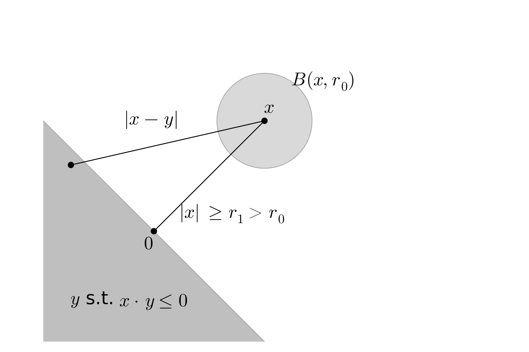
Figure 1: Sets used of the proof of Lemma 4.9

Since $x\cdot y\leq 0$ then $|x-y|^{2}=|x|^{2}+|y|^{2}-2x\cdot y\geq|x|^{2}$ and since $w$ is non-decreasing

$$\geq\int_{|x|\geq r_{1}}\int_{y\cdot x\leq 0}w(|x|)\rho(x)\rho(y)\mathop{}\!\mathrm{d}y\mathop{}\!\mathrm{d}x$$

$$\geq\int_{|x|\geq r_{1}}w(|x|)\rho(x)\int_{y\cdot x\leq 0}\rho(y)\mathop{}\!\mathrm{d}y\mathop{}\!\mathrm{d}x.$$

Since $\rho$ is radially symmetric, for any $x\in{\mathbb{R}^{d}}$ we have

$$\int_{y\cdot x\leq 0}\rho(y)\mathop{}\!\mathrm{d}y=\frac{1}{2}\int_{{\mathbb{R}^{d}}}\rho(y)\mathop{}\!\mathrm{d}y.\qed$$

4.2.3 An $L^{p}$ estimate

We can proceed similarly to the approach in (4.5) in more general settings. If we drop the term coming from the diffusion, then we get

$$\frac{\mathop{}\!\mathrm{d}}{\mathop{}\!\mathrm{d}t}\frac{1}{p}\int_{\omega}\rho^{p} =\int_{\omega}\rho^{p-1}\frac{\partial\rho}{\partial t}$$

$$=\int_{\omega}\rho^{p-1}\operatorname{div}\rho\nabla\frac{\delta{\mathcal{F}}}{\delta\rho}$$

$$=-(p-1)\int_{\omega}\rho^{p-1}\nabla\rho\nabla(U^{\prime}(\rho)+V+{\mathcal{K}}\rho)+\int_{\partial\omega}\rho^{p}\nabla\frac{\delta{\mathcal{F}}}{\delta\rho}\cdot n$$

$$\leq-\frac{p-1}{p}\int_{\omega}\nabla{\rho_{t}^{p}}\nabla(V+{\mathcal{K}}\rho)+\int_{\partial\omega}\rho^{p}\nabla\frac{\delta{\mathcal{F}}}{\delta\rho}\cdot n$$

Integrating by parts one final time leads to

$$\frac{\mathop{}\!\mathrm{d}}{\mathop{}\!\mathrm{d}t}\frac{1}{p}\int_{\omega}\rho^{p}\leq\frac{p-1}{p}\int_{\omega}\rho^{p}\Delta(V+{\mathcal{K}}\rho)-\frac{p-1}{p}\int_{\partial\omega}\rho^{p}\nabla(V+{\mathcal{K}}\rho)\cdot n(x)+\int_{\partial\omega}\rho^{p}\nabla\frac{\delta{\mathcal{F}}}{\delta\rho}\cdot n.$$ (4.7)

If we work in ${\mathbb{R}^{d}}$ with $V,W\in W^{2,\infty}$, we assume good decay of $\rho^{p}\nabla(V+{\mathcal{K}}\rho)$ and $\rho^{p}\nabla\frac{\delta{\mathcal{F}}}{\delta\rho}$ then the boundary term vanish and we can write an inequality for equation of the form

$$\|\rho_{t}\|_{L^{p}({\mathbb{R}^{d}})}\leq\|\rho_{0}\|_{L^{p}({\mathbb{R}^{d}})}e^{Ct}.$$

However, when we work in $\Omega$ with (BC^∗) and we take $\omega=\Omega$, then the last term vanishes. However, we cannot relate the boundary term $\rho^{p}\nabla(V+{\mathcal{K}}\rho)\cdot n(x)$ to the $L^{p}$ norm of $\rho$. In some cases it can be compensated by the negative diffusion term, but not in general. This is one of the reasons we assume (2.7) on the boundary.

4.2.4 Free-energy dissipation

Definition 4.10 (First variation).

Let $X$ be a normed space, ${\mathcal{F}}:X\to\mathbb{R}$ and fix $\rho_{0}\in X$. We say ${\mathcal{F}}$ it is Gateaux differentiable at $X$ if for all $\varphi\in X$ there exists

$$\mathop{}\!\mathrm{d}{\mathcal{F}}[\rho_{0},\varphi]\vcentcolon=\lim_{\varepsilon\to 0}\frac{{\mathcal{F}}[\rho_{0}+\varepsilon\varphi]-{\mathcal{F}}[\rho_{0}]}{\varepsilon}.$$

The function $\mathop{}\!\mathrm{d}{\mathcal{F}}$ is usually called first variation of ${\mathcal{F}}$. Some authors extend this definition and require just that the limit exists for $\varphi$ in a dense subset of $X$. Functionals that admit first variation are called Gateaux differentiable.

When $X\subset L^{1}(\Omega)$, the first variation can sometimes be represented by a function $f_{0}\in L^{1}(\Omega)$ the sense that

$$\int_{\Omega}f_{0}(x)\varphi(x)\mathop{}\!\mathrm{d}x=\mathop{}\!\mathrm{d}{\mathcal{F}}[\rho_{0},\varphi],\qquad\forall\varphi\in L^{\infty}(\Omega).$$

If this is the case, we denote $\frac{\delta F}{\delta\rho}[\rho_{0}]\vcentcolon=f_{0}$. It is easy to check formally that, when $\mathcal{F}$ is given by (FE^∗) and $K(x,y)=K(y,x)$, then (2.9). In many of the examples the first variation can be rigorously computed.

If $K(x,y)=K(y,x)$ then the solutions of (ADE^∗) admits (FE^∗) as Lyapunov functional. This functional is usually called free energy. For smooth solutions of (ADE^∗) (with sufficiently good decay as $|x|\to\infty$ in unbounded domains) we can compute

$$\frac{\mathop{}\!\mathrm{d}}{\mathop{}\!\mathrm{d}t}\mathcal{F}[\rho]=-\int_{\Omega}\rho\left|\nabla\frac{\delta\mathcal{F}}{\delta\rho}\right|^{2}+\int_{\partial\Omega}\rho\nabla\frac{\delta\mathcal{F}}{\delta\rho}\cdot n.$$ (4.8)

When $\Omega={\mathbb{R}^{d}}$ (with sufficiently good decay of $\rho\nabla\frac{\delta\mathcal{F}}{\delta\rho}[\rho_{t}]$) or we have the no-flux condition (BC^∗), we recover the decay of the free energy, i.e., along solutions of (ADE^∗) we have decay of free-energy dissipation

$$\mathcal{F}[\rho_{t}]-\mathcal{F}[\rho_{s}]=-\int_{s}^{t}\int_{\Omega}\rho\left|\nabla\frac{\delta\mathcal{F}}{\delta\rho}[\rho]\right|^{2}.$$ (4.9)

In particular if $s<t$ then ${\mathcal{F}}[\rho_{s}]>{\mathcal{F}}[\rho_{t}]$.

Remark 4.11.

Often the free energy dissipation allows us to prove tightness. One approach is to recall Remark 4.8 and notice that free energy dissipation includes a term $\int_{\Omega}V\rho$. The term $\iint W(x-y)\rho(x)\rho(y)$ can also be useful due to Lemma 4.9.

4.2.5 Negative Sobolev spaces

Given a set $\Omega$, the negative Sobolev spaces can be defined by distributions with finite norm

$$\|f\|_{W^{-1,1}(\Omega)}=\inf_{f=\operatorname{div}F}\|F\|_{L^{1}(\Omega)}$$

Using the free-energy dissipation

$$\Big{\|}\frac{\partial\rho_{t}}{\partial t} \Big{\|}_{W^{-1,1}(\Omega)}=\inf_{\frac{\partial\rho_{t}}{\partial t}=\operatorname{div}F}\|F\|_{L^{1}(\Omega)}\leq\|\rho\nabla\tfrac{\delta\mathcal{F}}{\delta\rho}\|_{L^{1}}$$

$$\leq\|\rho_{t}\|_{L^{1}}^{\frac{1}{2}}\left(\int_{\Omega}\rho_{t}\left|\nabla\tfrac{\delta\mathcal{F}}{\delta\rho}\right|^{2}\right)^{\frac{1}{2}}=\|\rho_{t}\|_{L^{1}}^{\frac{1}{2}}\left(-\frac{d}{dt}\mathcal{F}[\rho_{t}]\right)^{\frac{1}{2}}$$

Also $\|\rho_{t}\|_{L^{1}}\leq\|\rho_{0}\|_{L^{1}}$. In the smooth setting, we can integrate in time

$$\|\rho_{t}-\rho_{s}\|_{W^{-1,1}}\leq C|t-s|^{\frac{1}{2}}(\mathcal{F}[\rho_{s}]-\mathcal{F}[\rho_{t}])^{\frac{1}{2}}.$$

Since $L^{1}$ is compactly embedded in $W^{-1,1}$, when ${\mathcal{F}}$ is bounded below, the sequence

$$\rho^{[n]}_{t}=\rho_{n+t}$$

is relatively compact in $C([0,1];W^{-1,1}(B_{R}))$ due to Ascoli-Arzelá theorem. Let $\widehat{\rho}\in W^{-1,1}$ be the limit of a sub-sequence. Since $\mathcal{F}[\rho_{t}]$ is bounded below and non-increasing, there is a limit $\widehat{\mathcal{F}}$. Then

$$\|\widehat{\rho}_{t}-\widehat{\rho}_{s}\|_{W^{-1,1}}\leq C|t-s|^{\frac{1}{2}}(\widehat{\mathcal{F}}-\widehat{\mathcal{F}})=0.$$

So $\widehat{\mu}$ does not depend on $t$. In the cases where one can prove stronger convergences, it can be shown that it is a stationary solution, i.e.,

$$\operatorname{div}\left(\widehat{\rho}\nabla\frac{\delta\mathcal{F}}{\delta\rho}[\widehat{\rho}]\right)=0.$$ (4.10)

4.3 Optimal-transport approach: Wasserstein spaces and the JKO scheme

As we already mentioned in Section 4.1.4, there is a clear connection between some of our equations and Optimal Transport problems. Otto realised in [Ott96a] (see also [Ott01a]) that the (PME) in ${\mathbb{R}^{d}}$ corresponds, in fact, to the gradient flow of a $\mathcal{F}$ with respect to the 2-Wasserstein distance. This idea led to the so-called “Otto calculus” that was later perfected.

The following pages are meant as an extremely brief introduction. For the reader interested in deepening their understanding of these spaces and their connection to PDEs we suggest reading the lecture notes [ABS21a] first, and then the very detailed books [AGS05a, Vil09a]. A very nice presentation with an emphasis on the examples can be found in [San15a].

4.3.1 The Wasserstein distances

The Wasserstein metrics were a tool already used by people studying optimal transport between probability measures. We give a brief definition. Let $X$ be a metric space with a Borel algebra, and recall the definition of push-forward given in Section 4.1.4. If we are given $\mu,\nu\in\mathcal{P}(X)$, a transport map is a measurable function $T$ such that $\nu=T_{\sharp}\mu$. We can formally think about the $p$-Wasserstein distance between probability distributions are defined for $p\geq 1$ as

$$\left(\inf_{T:\nu=T_{\sharp}\mu}\int_{X}|x-T(x)|^{p}\mathop{}\!\mathrm{d}\mu(x)\right)^{\frac{1}{p}}$$ (4.11)

This is the so-called Monge optimisation problem. The infimum is not always achieved, and sometimes no valid $T$ exists. Kantorovich improved this idea by introducing transport plans. A transport plan is a probability distribution in $\mathcal{P}(X\times X)$ that have $\mu,\nu$, i.e.,

$$\mu(A)=\pi(A\times X),\qquad\nu(A)=\pi(X\times A),\qquad\text{ for all }A\subset X\text{ measurable}.$$

This set is denoted by $\Pi(\mu,\nu)$, and is never empty because of the measure $\mu\otimes\nu\in\Pi(\mu,\nu)$, the unique measure such that

$$(\mu\otimes\nu)(A\times B)=\mu(A)\nu(B).$$

The Wasserstein distances are defined as

$${\mathfrak{W}}_{p}(\mu,\nu)\vcentcolon=\left(\min_{\pi\in\Pi(\mu,\nu)}\iint_{X\times X}|x-y|^{p}\mathop{}\!\mathrm{d}\pi(x,y)\right)^{\frac{1}{p}}.$$ (4.12)

These distances are sometimes called also Kantorovich-Rubinstein distance. The distance between two measures in $\mathcal{P}(X)$ can be infinite, unless the finite $p$-th order moment is finite. Hence, we define the $p$-Wasserstein space

$$\mathcal{P}_{p}(X)\vcentcolon=\left\{\mu\in\mathcal{P}(X):\int_{X}|x|^{p}\mathop{}\!\mathrm{d}\mu(x)<\infty\right\}.$$

The pair $(\mathcal{P}_{p}(X),{\mathfrak{W}}_{p})$ is a metric space. If $X$ is complete, then so this is space is also complete and it is equivalent to the narrow convergence (see [AGS05a, Proposition 7.1.5]). This is why we pick $X=\overline{\Omega}$.

As it usually happens in these families of spaces, there are three highlighted cases: $p=1,2,\infty$. The case $p=2$ will appear in the next section, and it is the one directly related to (ADE). The advantage of $p=1$ is the so-called Kantorovich-Rubinstein duality

$${\mathfrak{W}}_{1}(\mu,\nu)=\sup\left\{\int\psi\mathop{}\!\mathrm{d}\mu-\int\psi\mathop{}\!\mathrm{d}\nu:\text{for }\psi\text{ such that }\sup_{x\neq y}\frac{|\psi(x)-\psi(y)|}{|x-y|}\leq 1\right\}.$$ (4.13)

A very interesting property of the Wasserstein distance is that it admits a dynamic characterisation through the so-called Benamou-Brenier formula which is stated easiest in ${\mathbb{R}^{d}}$

$${\mathfrak{W}}_{2}(\mu_{0},\mu_{1})=\inf_{(\mu,v)\in\mathcal{A}(\mu_{0},\mu_{1})}\int_{0}^{1}\int_{\mathbb{R}^{d}}|v_{t}|^{2}\mathop{}\!\mathrm{d}\mu_{t}\mathop{}\!\mathrm{d}t,$$ (4.14)

where

$$\mathcal{A}(\mu_{0},\mu_{1})=\Big{\{}(\mu,\nu) :\mu\in C([0,1],\mathcal{P}_{2}({\mathbb{R}^{d}})),v\in L^{2}([0,1]\times\mathbb{R}^{d},\mu)^{d},$$

$$\qquad\mu(0)=\mu_{0},\mu(1)=\mu_{1}\text{, and }\frac{\partial\mu_{t}}{\partial t}+\operatorname{div}(\mu_{t}v_{t})=0\Big{\}}$$

is set space of admissible paths between $\mu_{0}$ and $\mu_{1}$.

4.3.2 Otto’s calculus

The notion of calculus in these spaces is a little tricky, since $\mathcal{P}_{p}({\mathbb{R}^{d}})$ are not vector spaces. However, they are subsets of the linear space of measures. In fact, it can be though of as a manifold: we can define tangent through curves. In particular, $\rho_{0}\in\mathcal{P}_{2}({\mathbb{R}^{d}})$ and take $\varphi\in C_{c}^{\infty}({\mathbb{R}^{d}})$ a test function. Consider the curve of probabilities

$$\rho_{t}=(\mathrm{id}+t\nabla\varphi)_{\sharp}\rho_{0}.$$

It is not too difficult to see [ABS21a, Lecture 16] that $\rho_{t}$ is a distributional solution of the continuity equation

$$\frac{\partial\rho_{t}}{\partial t}+\operatorname{div}(\rho_{t}v_{t})=0$$

where $v_{t}=\nabla\varphi\circ(\mathrm{id}+t\nabla\varphi)^{-1}$. Then formally the tangent space $T_{\rho_{0}}\mathcal{P}_{2}({\mathbb{R}^{d}})$ is made of

$$s\vcentcolon=\frac{\mathop{}\!\mathrm{d}}{\mathop{}\!\mathrm{d}t}\Big{|}_{t=0}\rho_{t}=-\operatorname{div}(\rho_{t}\nabla\varphi).$$

This allows to formally construct the gradient of functions. Take the free energy of the diffusion term $\mathcal{U}$. In distributional sense the Wasserstein gradient is

$$\langle\nabla_{{\mathfrak{W}}_{2}}U[\rho_{0}],s\rangle \vcentcolon=\frac{\mathop{}\!\mathrm{d}}{\mathop{}\!\mathrm{d}t}\Big{|}_{t=0}\mathcal{U}[\rho_{t}]=\int_{\mathbb{R}^{d}}U^{\prime}(\rho_{0})\frac{\partial}{\partial t}\Big{|}_{t=0}\rho_{t}$$

$$=-\int_{\mathbb{R}^{d}}U^{\prime}(\rho_{0})\operatorname{div}(\rho_{0}\nabla\varphi)$$

$$=-\int_{\mathbb{R}^{d}}\varphi\operatorname{div}(\rho_{0}\nabla U^{\prime}(\rho_{0})).$$

In general

$$\langle\nabla_{{\mathfrak{W}}_{2}}\mathcal{F}[\rho_{0}],s\rangle=-\int_{\Omega}\varphi\operatorname{div}\left(\rho\nabla\frac{\delta\mathcal{F}}{\delta\rho}[\rho_{0}]\right)$$ (4.15)

Hence, (ADE) in ${\mathbb{R}^{d}}$ is formally written can be formally written as the $2$-Wasserstein gradient flow in the sense that

$$\frac{\partial\rho}{\partial t}=-\nabla_{{\mathfrak{W}}_{2}}\mathcal{F}[\rho_{t}]$$

of the free energy given by (FE).

Remark 4.12.

If we work in a bounded domain, then we must study the space $\mathcal{P}_{2}(\overline{\Omega})$ and understand how the no-flux condition (BC) appears naturally in this context. One approach is to consider $\varphi\in C_{c}^{\infty}(\overline{\Omega})$ (meaning their support is bounded and does not reach the boundary). In order for $\mathrm{id}+t\nabla\varphi:\overline{\Omega}\to\overline{\Omega}$ when $t\in(-\varepsilon,\varepsilon)$ we must specify $\rho\nabla\varphi\cdot n=0$. This is related to how the no-flux appears. We will continue this discussion below in Remark 4.13.

4.3.3 Rigorous gradient flow structure. The JKO scheme

The idea of writing gradient flows in terms of minimising movements is due to De Giorgi (see [De ̵93a]). To draw a quick analogy think that we can to minimise a function $F:\mathbb{R}^{d}\to\mathbb{R}$. A continuous ODE going to local minimima is the ${\mathbb{R}^{d}}$ gradient flow

$$\frac{\mathop{}\!\mathrm{d}x}{\mathop{}\!\mathrm{d}t}=-\nabla F(x)$$

The implicit Euler scheme leads to the implicit gradient-descent method

$$\frac{x_{n+1}-x_{n}}{\tau}=-\nabla F(x_{n+1}).$$

We have avoided making explicit the dependence of $x_{n}$ with respect to $\tau$. We can rewrite this the minimisation of the so-called proximal function

$$x_{n+1}=\operatorname*{argmin}_{x\in{\mathbb{R}^{d}}}\left(\frac{|x-x_{n}|^{2}}{2}+\tau F(x)\right)$$ (4.16)

If $F$ is smooth this minimisation problem has a unique solution for $\tau$ small. These are the so-called minimising movements. Then one can do a piece-wise constant interpolation $x^{(\tau)}(t)\vcentcolon=x_{n}$ when $t\in[\tau n,\tau(n+1))$, or even linear interpolation.

The notion of minimising movement can be generalised to metric spaces and, in particular, we can construct in $2$-Wasserstein space

$$\mu_{n+1}=\operatorname*{argmin}_{\mu\in\mathcal{P}_{2}({\mathbb{R}^{d}})}\left(\frac{{\mathfrak{W}}_{2}(\mu,\mu_{n})^{2}}{2}+\tau\mathcal{F}(\mu)\right).$$ (4.17)

Jordan, Kinderlehrer, and Otto proved in the seminal paper [JKO98a] that this procedure works for (HE-FP). The book [AGS05a] is devoted to proving how these minimising movements lead to (ADE) in ${\mathbb{R}^{d}}$ for fairly general $\mathcal{F}$. A good notion of solution for the limit of minimising movements is that of curves of maximal slope. Often, it is even possible to get back a suitable solution of a PDE.

Remark 4.13.

In bounded domains, we continue the comment in Remark 4.12. In general, if one minimises over $\mathcal{P}_{2}(\overline{\Omega})$, then we expect to arrive (ADE) with the no-flux condition (BC^∗). We recommend [San15a, Chapter 8].

However, the general setting is tricky as presented by the following example.

Remark 4.14.

Take $\Omega=(-1,1)$ (i.e., $d=1$), $U=W=0$ and $V(x)=ax$. Then we recover the transport equation $\frac{\partial\rho}{\partial t}=a\frac{\partial\rho}{\partial x}$. The solutions of this equation are always of the form $\rho(t,x)=\rho_{0}(x+at)$. The boundary condition $a\rho=0$ can be forced on one side, but never the other. From the perspective below one can always consider a Dirac delta on the right-hand side. This negates somehow $a\rho=0$ on that side, but it is only possible solution. In fact, it is recovered from the vanishing viscosity formulation.

Notice that this examples does not satisfy (2.7). If we replaced $V$ by a different smooth potential such that (2.7), then the characteristics will not reach the boundary in finite time. Hence, we will expect a smooth solution.

Remark 4.15.

Otto’s original paper [Ott96a] already covered $p$-Wassersten distances with $p\neq 2$. In particular, it showed that the doubly nonlinear equation

$$\frac{\partial u}{\partial t}=\Delta_{p}u^{m}$$

has a $p$-Wasserstein gradient-flow structure. Recently, a new article has appeared justifying the JKO scheme for these problems, see [CS24b].

4.3.4 Convexity and McCann’s condition

In the same way that (4.16) works better if $F:{\mathbb{R}^{d}}\to\mathbb{R}$ is convex, there is a suitable notion of convexity that works for (4.17). The correct extension is convexity along geodesics also called displacement convexity, i.e., if $\rho_{t}$ is a geodesic from $\rho_{0}$ to $\rho_{1}$ then $t\mapsto\mathcal{F}[\rho_{t}]$ is a convex $[0,1]\to\mathbb{R}$ function. It is usually called displacement convexity and was introduced by McCann in [McC97a].

Before we present this result, it is interesting to discuss the structure of geodesics in Wasserstein space (see, e.g., [ABS21a]). As the simplest case, assume that $\mu,\nu$ are absolutely continuous probability distributions and compactly supported. Then, Monge’s problem (4.11) for $p=2$ admits an optimal transport map $T=\nabla\varphi$ such that $\nu=T_{\sharp}\mu$ (see, e.g., [ABS21a, Lecture 5]). Furthermore, the unique geodesic between $\mu$ and $\nu$ is given by

$$\rho_{t}=((1-t)\mathrm{id}+tT)_{\#}\mu.$$

In [McC97a] the author proves that if $V,W$ are strictly convex, $W(x)=W(-x)$ then

$$\int_{\mathbb{R}^{d}}V\rho,\qquad\iint_{{\mathbb{R}^{d}}\times{\mathbb{R}^{d}}}W(x-y)\rho(x)\rho(y)\mathop{}\!\mathrm{d}x\mathop{}\!\mathrm{d}y$$

are displacement convex. For the diffusion term there is a more interesting condition, known as McCann’s condition. It states that if we define

$$P^{\prime}(s)\vcentcolon=sU^{\prime}(s),\qquad P(0)\vcentcolon=0$$

then (2.11) is displacement convex if and only if

$$P^{\prime}(s)s\geq(1-1/d)P(s)\geq 0,\qquad\forall s\in(0,\infty).$$ (4.18)

This can also be written as $\lambda\mapsto\lambda^{d}U(\lambda^{-d})$ is convex. When $U=\frac{s^{m}}{m-1}$ this means $m\geq\frac{d-1}{d}$.

Remark 4.16.

The case $m>\frac{d-1}{d}$ and $V(x)=\frac{|x|^{2}}{2}$ the functional is $0$-convex and bounded below. But recalling Remark 3.2 for $m<\frac{d}{2+d}$ the (3.2) is not in $\mathcal{P}_{2}$, we cannot hope for asymptotic convergence in 2-Wasserstein sense.

Besides “regular” convexity, a powerful tool in the arsenal is the notion of $\lambda$-convexity. A function $f:(0,1)\to\mathbb{R}$ is $\lambda$-convex if $f(t)-\lambda\frac{|t|^{2}}{2}$ is convex. Analogously as above we introduce the notion of displacement (or geodesically) $\lambda$-convex. In this setting for the gradient flow starting from two points we have

$${\mathfrak{W}}_{2}(\mu_{t},\widehat{\mu}_{t})\leq e^{-\lambda t}{\mathfrak{W}}_{2}(\mu_{0},\widehat{\mu}_{0}).$$

This implies uniqueness of the gradient flow and, if $\mathcal{F}$ is bounded below, of its minimisers.

A similar analysis of a free energy in $\mathbb{S}^{1}$ is done in [CS09a]. The sense in which the equation is satisfied is delicate. For $U=V=0$ and $W$ “pointy”, we send the reader to [CDFLS11a].

4.4 Global existence vs finite-time blow-up

As explained above, local-in-time existence is usually achieved through “standard” PDE methods or the use of gradient flow arguments, specially if starting from a nice initial datum $\rho_{0}$. Whether these solutions behave “nicely” for large $t$ is a more difficult problem.

Transport for given potential

Going back to the simplest example (CE) we can look at the examples $V=\frac{|x|^{\alpha}}{\alpha}$ with $\alpha>0$. Then $v=-\nabla V=-|x|^{\alpha-2}x$ and $\rho_{t}=(X_{t})_{\sharp}\rho_{0}$ with corresponding characteristic field is obtained by solving

$$\frac{\partial X_{t}}{\partial t}=-|X_{t}|^{\alpha-2}X_{t},$$

with $X_{t}(0)=y$. We conclude that

$$X_{t}(y)=\begin{dcases}ye^{-t}&\text{if }\alpha=2,\\ (|y|^{2-\alpha}-(2-\alpha)t)^{\frac{1}{2-\alpha}}\frac{y}{|y|}&\text{if }\alpha\neq 2.\end{dcases}$$

For $\alpha<2$ the characteristics arrive at $0$ at finite time and hence we get a Dirac delta at $0$ at a certain finite time for any $\rho_{0}\not\equiv 0$. This is not problematic in the distributional sense in this case. However, this behaviour happens also for other problems.

Keller-Segel problem.

Some authors noticed by direct techniques that the Keller-Segel model has finite-time blow-up for initial data with large enough mass. [JL92a] showed for (KSE) in a bounded domain with no-flux the existence of a critical mass $M^{*}$ such that, if $\|\rho_{0}\|_{L^{1}}>M^{*}$, then $\rho(T^{*})$ contains a Dirac delta. Later this result was obtained also in ${\mathbb{R}^{d}}$ in [HV96a] using radial arguments, where the authors characterise the critical mass is $M^{*}=8\pi$. This was later proved in more generality in [DP04a]. Conversely, for $\|\rho_{0}\|_{L^{1}}<M^{*}$ global existence for (KSE) is known. In $d=2$ it was shown in [BDP06a].

A nice proof of the formation of a Dirac comes through the analysis of the second-order moment. For (KSE) in $d=2$ it was first noticed by [DP04a] that, working with solutions of initial mass $\int_{\mathbb{R}^{d}}\rho_{0}=M$,

$$\frac{\mathop{}\!\mathrm{d}}{\mathop{}\!\mathrm{d}t}\int_{\mathbb{R}^{d}}|x|^{2}\rho(t,x)\mathop{}\!\mathrm{d}x=4M\Big{(}1-\frac{M}{8\pi}\Big{)}.$$

Hence, if $M>{8\pi}$ necessarily the second-order moment becomes negative in finite time. This is incompatible with our non-negative solutions. There is complete concentration to a Dirac delta. This was later extended by [BCL09c] for (KSE) when $d>2$ where the authors prove that

$$\frac{\mathop{}\!\mathrm{d}}{\mathop{}\!\mathrm{d}t}\int_{\mathbb{R}^{d}}|x|^{2}\rho(t,x)\mathop{}\!\mathrm{d}x=2(d-2)\mathcal{F}[\rho(t,\cdot)]\leq 2(d-2)\mathcal{F}[\rho_{0}].$$

When $M>M^{*}$, there exist $\|\rho_{0}\|_{L^{1}}=M$ such that $\mathcal{F}[\rho_{0}]<0$. We will perform the analysis of the free energy for this problem in Remark 6.15. We will discuss below in Section 5.1.3 the critical case $M=8\pi$ and some interesting ad-hoc constructions which are available in the literature.

5 Asymptotics

The aim of this section is to highlight some techniques coming from the PDE community that allow us to understand the behaviour as $t\to\infty$ (and sometimes $|x|\to\infty$) of “typical” solutions of the problem (namely those with “good” initial values).

5.1 Self-similarity

Some of the equations we are analysing have linear operators homogeneous non-linearities, and it is therefore interesting to exploit this structure. One of the main approaches comes from considering the mass-preserving change of variable

$$u(\tau,y)=\sigma(\tau)^{d}\rho\Big{(}\tilde{t}(\tau),\sigma(\tau)y\Big{)}.$$ (5.1)

5.1.1 Self-similar scaling for (PME)

Let $\rho$ be the solution of (PME). Applying the chain rule to (5.1)

$$\frac{\partial u}{\partial\tau} =\frac{\frac{\mathop{}\!\mathrm{d}\sigma}{\mathop{}\!\mathrm{d}\tau}}{\sigma}u\operatorname{div}_{y}y+\sigma^{d}\frac{\mathop{}\!\mathrm{d}\sigma}{\mathop{}\!\mathrm{d}\tau}\nabla_{x}\rho\cdot\nabla_{y}y+\sigma^{d}\frac{\mathop{}\!\mathrm{d}\tilde{t}}{\mathop{}\!\mathrm{d}\tau}\Delta_{x}\rho^{m}$$

since $\nabla_{x}x=(1,\cdots,1)=\nabla_{y}y$ y $\operatorname{div}_{x}x=d=\operatorname{div}_{y}y$. Due to the chain rule

$$\frac{\partial u}{\partial y_{i}} =\sigma^{d+1}\frac{\partial\rho}{\partial x_{i}},\qquad\qquad\frac{\partial^{2}u^{m}}{\partial y_{i}^{2}}=\sigma^{2+md}\frac{\partial^{2}\rho^{m}}{\partial x_{i}^{2}}$$

Eventually, we simplify the equation for $u$ to

$$\frac{\partial u}{\partial\tau} =\frac{\frac{\mathop{}\!\mathrm{d}\sigma}{\mathop{}\!\mathrm{d}\tau}}{\sigma}\operatorname{div}_{y}(uy)+\sigma^{-d(m-1)+2}\frac{\mathop{}\!\mathrm{d}\tilde{t}}{\mathop{}\!\mathrm{d}\tau}\Delta_{x}\rho^{m}$$

The only sensible choice is $\frac{\mathop{}\!\mathrm{d}\sigma}{\mathop{}\!\mathrm{d}\tau}=\sigma$ and $\frac{\mathop{}\!\mathrm{d}\tilde{t}}{\mathop{}\!\mathrm{d}\tau}=\sigma^{\frac{1}{\kappa}}$ where $\kappa=(d(m-1)+2)^{-1},$ so we arrive to the simplified equation

$$\frac{\partial u}{\partial\tau} =\operatorname{div}_{y}(uy)+\Delta_{y}u^{m}.$$

Forward self-similar solutions

Notice that adding the condition $\sigma(0)=1$ we get $\sigma(\tau)=e^{\tau}$. We also have that $\frac{\mathop{}\!\mathrm{d}\tilde{t}}{\mathop{}\!\mathrm{d}\tau}=e^{\tau/\kappa}$. We have $t=\tilde{t}(\tau)$ so we set $\tilde{t}(0)=0$. Eventually

$$t =\frac{e^{\frac{\tau}{\kappa}}-1}{\kappa}$$

$$\kappa =(d(m-1)+2)^{-1}$$

$$x =e^{\tau}y.$$

Notice that $\kappa>0$ if and only if $m>m_{c}=\frac{d-2}{d}$. The Barenblatt solution (ZKB) corresponds to setting $u$ as stationary. In fact, for $m>m_{c}$ we can write the family of self-similar solutions

$$\rho_{t}(x) \vcentcolon=\frac{1}{\sigma_{B}(t+T)^{d}}F\left(\frac{x}{\sigma_{B}(t+T)}\right),$$

$$F_{B}(y) \vcentcolon=\left(D-\frac{m-1}{2m}|y|^{2}\right)^{\frac{1}{m-1}}_{+}$$

$$\sigma_{B}(t) \vcentcolon=(d|m-m_{c}|t)^{\frac{1}{d(m-m_{c})}}.$$

Here we have chosen the presentation in [CT00a, BBDGV09a].

Backwards self-similar solutions

When $\kappa<0$ (i.e., $m>m_{c}=\frac{d-2}{d}$), we can build another type of solution. In [Váz06b, Section 5.2], Vázquez introduces the pseudo-Barenblatt solutions for the sub-critical regime $0<m<m_{c}$ which can be written

$$\rho_{t}(x) \vcentcolon=\frac{1}{\sigma_{B}(T-t)^{d}}F_{B}\left(\frac{x}{\sigma_{B}(T-t)}\right).$$

Here, $T$ denotes the extinction time. They are suitable to deal with finite-time extinction [BBDGV09a].

5.1.2 Self-similar analysis in more general contexts

In the previous computation we can trade $\Delta_{x}\rho^{m}$ for any non-linear operator $\mathcal{L}$ with the scaling property

$$\mathcal{L}[u]=\sigma^{q}\mathcal{L}[\rho].$$

Self-similarity analysis for (CVE) was performed in [CV11c, Theorem 3.1]. The result passes by an obstacle problem. For (NVE) the self-similar analysis is done in [SV14a, Section 6.2]. For the fractional heat equation see [GI08a].

Self-similar solutions are very particular of problem where all terms have the same scaling, and it is not reasonable to expect solutions of this nature to exist in general. Consider the problem

$$\frac{\partial\rho}{\partial t}=\mathcal{L}\rho.$$

When $\mathcal{L}$ is the sum of two terms with different scaling, it is not reasonable to expect self-similar structure. For (ADE) with $U=U_{m},V=0,W=W_{k}$ this is only possible in the so-called fair-competition regime

$$d(m-1)+k=0.$$

The self-similar analysis in this setting was performed in [CCH17a].

5.1.3 The Keller-Segel problem: bubbles

For $d=2$ a self-similar solution is not available, although [HV96a] give some hints on the shape by matching asymptotics. Later, there were more advanced studies on stability [Vel02a, Vel04b, Vel04c]. In this direction, see also [RS14a, CGMN22a].

In [HMV98a] the authors prove there are no self-similar solution of (KSE_χ) when $d=2$. However, for $d=3$ they show that there exists a sequence of radial self-similar solutions $\rho^{(n)}$

$$\rho^{(n)}_{t}(x)=\frac{1}{T-t}F_{n}\left(\frac{x}{\sqrt{T-t}}\right),\qquad\qquad\text{where }F_{n}(y)\sim\left(\frac{8\pi}{\chi}+a_{n}\right)\frac{1}{4\pi|y|^{2}}\text{ for }|y|\sim 0,$$

and $a_{n}\to 0$. This construction was later generalised for $d\geq 3$ by several authors [Sen05a, GMS11a, SW19a]. Blow-up on the range $U=U_{m}$ for $m\geq 1$, $V=0$ and $W=W_{k}$ with $k>2-d$ see [YB13a].

It was later conjectured in [Pin17a] and proved in [DPDMWa] that for $d=2$ one can construct “approximate bubbles”. In particular, an initial datum $\rho_{0}^{\star}$ with initial mass $8\pi$ so that the solutions of Keller-Segel problem (KSE) such that, for $\rho_{0}$ close to $\rho_{0}^{\star}$

$$\rho(t,x)\approx\frac{1}{\sigma(t)^{2}}F\left(\frac{x-\chi(t)}{\sigma(t)}\right),\qquad F(y)=\frac{8}{(1+|y|^{2})^{2}}$$

as $t\to\infty$ where $\sigma(t)\approx c/\sqrt{\log t}$, $\chi(t)\to q$.

5.2 Relative entropy

If we are able to construct a global solution $B_{t}$ of which we know some properties, we would like to see whether this is the “generic behaviour”. Assume we are in a case where $\|\rho_{t}\|_{L^{1}}$ is preserved. We would say that $B_{t}$ is attractive if

$$\|\rho_{t}-B_{t}\|_{L^{1}}\to 0,\qquad\text{as }t\to\infty.$$

For $L^{p}$ norms in general (which typically change over time), we would to see if the relative error tends to zero

$$\frac{\|\rho_{t}-B_{t}\|_{L^{p}}}{\|\rho_{t}\|_{L^{p}}}\to 0,\qquad\text{as }t\to\infty.$$ (5.2)

These are usually called intermediate asymptotics, as opposed to the long-time asymptotic limit.

Naïve computations do not yield good results. Sometimes it is possible to do this computation directly via comparison arguments. But, in general, this is not possible. A useful tool is are the so-called relative entropies. We start by a simple example, (HE).

5.2.1 $L^{2}$ relative entropy for (HE)

An interesting alternative way of writing (HE-FP) as

$$\frac{\partial u}{\partial t}=\operatorname{div}\left(G\nabla\frac{u}{G}\right),$$

where $G$ is the Gaussian profile (3.1). Let us take $w=\tfrac{u}{G}$ we rewrite this problem as

$$\frac{\partial w}{\partial t}=G^{-1}\operatorname{div}\left(G\nabla w\right)=\Delta w-x\cdot\nabla w.$$

This is the famous Ornstein-Uhlenbeck problem, which is also the dual (HE-FP). We can write the free-energy dissipation formula

$$\frac{\mathop{}\!\mathrm{d}}{\mathop{}\!\mathrm{d}t}\int_{\mathbb{R}^{d}}|w-1|^{2}G\mathop{}\!\mathrm{d}x=-2\int_{\mathbb{R}^{d}}|\nabla w|^{2}G\mathop{}\!\mathrm{d}x.$$

We can now take advantage of the Gaussian Poincaré inequality, see [Che81a],

$$\int_{\mathbb{R}^{d}}w^{2}G\mathop{}\!\mathrm{d}x-\left(\int_{\mathbb{R}^{d}}wG\mathop{}\!\mathrm{d}x\right)^{2}\leq\int_{\mathbb{R}^{d}}|\nabla w|^{2}G.$$

Hence, assuming that $\int_{\mathbb{R}^{d}}wG=\int_{\mathbb{R}^{d}}u=1,$ we recover that

$$\int_{\mathbb{R}^{d}}|w_{t}-1|^{2}G\mathop{}\!\mathrm{d}x\leq e^{-2t}\int_{\mathbb{R}^{d}}|w_{0}-1|^{2}G\mathop{}\!\mathrm{d}x.$$

This approach can be generalised in many directions. We point the reader to [AMTU01a] and the references therein.

5.2.2 $L^{1}$ Relative entropy argument for (HE)

For convenience, we will denote the solution of (HE-FP) by $v$. Notice that, with our choice of re-scaling $v_{0}=\rho_{0}$. The relative entropy is defined

$$\mathcal{E}(v)=\int_{\mathbb{R}^{d}}v\log\frac{v}{G}=\int_{\mathbb{R}^{d}}v\left(\log v+\frac{x^{2}}{2}v\right)+C.$$

It is easy to check that

$$\frac{\mathop{}\!\mathrm{d}}{\mathop{}\!\mathrm{d}t}\mathcal{E}(v)=-\mathcal{I}(v),$$

where $\mathcal{I}$ is the so-called Fisher information

$$\mathcal{I}(v)=\int_{\mathbb{R}^{d}}v\left|\frac{\nabla v}{v}+x\right|^{2}=\int_{\mathbb{R}^{d}}v\left|\nabla\log\frac{v}{G}\right|^{2}.$$

The Gaussian logarithmic Sobolev inequality (see [Gro75a, Tos99a, DT15a])

$$\frac{1}{2}\int_{\mathbb{R}^{d}}(|f|^{2}\log|f|^{2})G\mathop{}\!\mathrm{d}x\leq\int_{\mathbb{R}^{d}}|\nabla f|^{2}G,\qquad\text{if }\int_{\mathbb{R}^{d}}|f|^{2}G=1.$$ (5.3)

This inequality ensures the relationship $\mathcal{E}\leq\tfrac{1}{2}\mathcal{I}$, and hence we recover an ordinary differential inequation that yields $\mathcal{E}(v_{t})\leq\mathcal{E}(\rho_{0})e^{-2t}$. Lastly, we will take advantage of the Czsizar-Kullback inequality taking $G=K_{1}$

$$\|f-G\|_{L^{1}}^{2}\leq 2\mathcal{E}(f).$$

Eventually, we deduce that if $\rho$ is a solution (HE)

$$\|\rho_{t}-K_{t}\|_{L^{1}}\leq\sqrt{2\mathcal{E}(\rho_{0})}t^{-\frac{1}{2}}.$$

Remark 5.1.

It is also worth point out that (5.3) is equivalent to the Euclidean log-Sobolev inequality, which in scale invariant form (see [Wei78a, DT15a]) given by

$$\frac{d}{2}\log\left(\frac{2}{\pi de}\int_{\mathbb{R}^{d}}|\nabla f|^{2}\right)\geq\int_{\mathbb{R}^{d}}|f|^{2}\log|f|^{2},\qquad\text{if }\int_{\mathbb{R}^{d}}|f|^{2}=1.$$ (5.4)

Notice that is usually applied to $f=\sqrt{\rho}$, and hence the condition is simply that $\rho\in L^{1}({\mathbb{R}^{d}})\cap{\mathcal{P}}({\mathbb{R}^{d}})$.

5.2.3 $L^{1}$ relative entropy for (PME)

In [CT00a, PD02a] the authors extend the relative-entropy study to $m>1$. Now we denote by $v$ the solution of (PME-FP). Suppose there exists $\hat{v}$ of suitable mass and define the relative entropy and the Fisher information

$$H(v)=\int_{\mathbb{R}^{d}}\left(\frac{2}{m-1}v^{m}+|x|^{2}v\right)\qquad\qquad I(v)=\int_{\mathbb{R}^{d}}v\left|x+\frac{m}{m-1}\nabla v^{m-1}\right|^{2}.$$

The suitable relative entropy for $m>1$ is $\mathcal{H}(u||\hat{u})=\mathcal{H}(u)-\mathcal{H}(\hat{u})$. This was later extended to more general families than (PME-FP) in [CJMTU01a]. This relative-entropy arguments rely heavy on Gagliardo-Nirenberg-Sobolev inequalities. In fact, there is a deep connection between the smoothing properties of (PME) and these types of inequalities (see, e.g., [PD02a]). In [BBDGV09a, BDGV10a] the authors develop the correct relative entropies and Fisher information functions to cover the cases $m<1$ with the correct re-scaling of the Barenblatt/pseudo-Barenblatt explained in Section 5.1.1.

Remark 5.2.

This kind of relative entropy arguments for diffusive problems (which do not have a natural stationary state) rely on the self-similar solution. It is possible to prove intermediate asymptotics without homogeneity or self-similarity techniques. For diffusive problems of the form $\frac{\partial\rho}{\partial t}=\Delta\Phi(\rho)$, a very nice analysis using Wasserstein spaces can be found in [CFT06a].

5.2.4 Relative entropy argument for (ADE)

The entropy arguments for (PME) are stable enough that allow some families of perturbations into the range (ADE). For $W=0$ and confining potentials see [CJMTU01a]. The reader may find information on the strictly displacement-convex free-energy functionals [CMV03a, CMV06a]. For (KSE_m,χ) with $m\in[1,2-\frac{2}{d}]$ (and, in fact, a larger family of $W$ radially decreasing), intermediate asymptotics in the sense (5.2) are obtained in [Bed11c]. In [CGYZ23a] the authors take advantage of relative entropy arguments to prove that in the case $U(\rho)=\rho\log\rho,V=0$ and $W$ smooth and bounded (5.2) with $p=1$ and $B_{t}=K_{t}$ (i.e., the heat kernel). See [CCS12a] for previous results in this direction.

5.3 Study of the mass variable of radial solutions

One of the significant limitations to prove the above results rigorously is the lack of regularity of $\rho$. Some regularity can be regained by passing to the so-called mass variable.

Let $d=1$. Assume $x\in\mathbb{R}$ and

$$M(t,x)=\int_{-\infty}^{x}\rho_{t}(y)\mathop{}\!\mathrm{d}y.$$ (5.5)

Integrating (ADE) we show that $M$ satisfies a PDE

$$\frac{\partial M}{\partial t} =\Phi^{\prime}\left(\frac{\partial M}{\partial x}\right)\frac{\partial^{2}M}{\partial x^{2}}+\frac{\partial M}{\partial x}\frac{\partial V}{\partial x}+\frac{\partial M}{\partial x}\frac{\partial}{\partial x}\left(W*\frac{\partial M}{\partial x}\right)$$

If $\Phi(s)=|s|^{m-1}s$ (PME for $\rho$), this is the $p$-Laplacian for $M$ with $p=m+1$. If $x\in\mathbb{R}^{d}$ with $d>1$ it is better to define the mass in volumetric coordinates

$$M(t,v)=\int_{A_{v}}\rho(t,x)\mathop{}\!\mathrm{d}x,\qquad\text{where }A_{v}=B(0,r)\text{ such that }|A_{v}|=v.$$

Then, if $\rho$ is radially, we recover for a weight $\kappa$

$$\frac{\partial M}{\partial t} =\kappa(v)^{2}\Phi^{\prime}\left(\frac{\partial M}{\partial v}\right)\frac{\partial^{2}M}{\partial v^{2}}+\kappa(v)^{2}\frac{\partial M}{\partial v}\frac{\partial V}{\partial v}+\kappa(v)^{2}\frac{\partial M}{\partial v}\frac{\partial}{\partial v}\left(W*_{{\mathbb{R}^{d}}}\frac{\partial M}{\partial v}\right)$$

This is a Hamilton-Jacobi type equation, and is well suited for the theory of viscosity solutions. In [CGV22c] the authors discuss the problem when $W=0$. They show that one can take advantage of stability properties of viscosity solutions to characterise the steady state. Since $\kappa(0)=0$ and $\kappa(v)>0$ for $v>0$, this equation can be used to show that for smooth $V$ and $W$ and radially symmetric $\rho$, singularities can only form at $x=0$. They also show that a Dirac may form, but only in the limit $t\to\infty$.

Many authors have taken advantage of this kind of idea in their arguments. For example, we point to [HMV98a, Sen05a, GMS11a, KY12a].

There is also an interesting connection between the mass variable and the Wasserstein distance for $\rho$. The simplest case states that if $\rho_{1},\rho_{2}\in\mathcal{P}(\mathbb{R})$, and $M_{i}$ are their primitives, then

$${\mathfrak{W}}_{1}(\rho_{1},\rho_{2})=\|M_{1}-M_{2}\|_{L^{1}(\mathbb{R})}.$$

A similar formula holds if $\rho_{i}\in\mathcal{P}({\mathbb{R}^{d}})$, and are radially symmetric.

The inverse of the mass function

Furthermore, if we consider the generalised inverse

$$M^{-1}(s)=\inf\{v\in[-\infty,\infty):M(v)\geq s\}$$

and $\rho_{1},\rho_{2}\in\mathcal{P}(\mathbb{R})$, and $M_{i}$ are their primitives, then

$${\mathfrak{W}}_{p}(\rho_{1},\rho_{2})=\|M_{1}^{-1}-M_{2}^{-1}\|_{L^{p}(0,1)}.$$

Interestingly, if $\rho(t,x)$ solves a conservation problem, we can also deduce and equation for $u(t,s)=M^{-1}(t,s)$. This equation is usually degenerate, but the coefficients do not depend on $s$ (see, e.g., [CHR20a]).

5.4 On the attractiveness of attractors

Relative entropy arguments allow us to show that the steady state (or energy minimiser) in $L^{1}$ is an attractor for a large range of equations: from (PME-FP) to all the examples discussed in Section 5.2.4.

A more difficult question is to understand the case where the energy minimiser may contain a singular part, e.g.,

$$\widehat{\mu}=\widehat{\rho}+(1-\|\widehat{\rho}\|_{L^{1}})\delta_{0},$$ (5.6)

and $\|\widehat{\rho}\|_{L^{1}}<1$. We will see an example in the aggregation dominated range (see Corollary 6.13 below). It is difficult to say whether a measure of this kind can be called a steady state, since it cannot be plugged into even the distributional formulation. If the energy is $\lambda$-displacemente convex, there is no doubt that the minimiser is a global attractor.

In [CGV22c] the authors prove that (ADE^∗) $m\in(0,1)$, $V$ smooth, and $K=0$, the solution converges to the free energy minimiser, even when this contains a singular part. In [CFGa] the authors use the mass to prove that for (ADE^∗) $m\in(0,1)$, in large class of $K$.

In the recent preprint [Biaa], covering (ADE) when $k=2-2s\in(2-d,0)$ and $m=\frac{2d}{d+2s}$ (part of the fair-competition regime described in Section 6.3.3) shows that there is an explicit steady state (given in (6.3) below), and solutions with $\|\rho_{0}\|_{L^{m}}>\|\widehat{\rho}\|_{L^{m}}$ have $\|\rho_{t}\|_{L^{m}}$ blow-up in finite time (and hence even we cannot study them in the distributional sense).

6 Minimisation of the free energy

As mentioned in Section 4.3.4, displacement $\lambda$-convexity with $\lambda>0$ guarantees exponential contraction with rate

$${\mathfrak{W}}_{2}(\mu_{t},\widehat{\mu}_{t})\leq e^{-\lambda t}{\mathfrak{W}}_{2}(\mu_{0},\widehat{\mu}_{0})$$

In particular, if $\widehat{\mu}$ is a global minimiser of $\mathcal{F}$ (which is unique by convexity), then the JKO schemes is stationary and so is the gradient flow. This means that

$${\mathfrak{W}}_{2}(\mu_{t},\widehat{\mu})\leq e^{-\lambda t}{\mathfrak{W}}_{2}(\mu_{0},\widehat{\mu})$$

Therefore, it is a global attractor with exponential rate. First, we will try to characterise the local minimisers using variational arguments. This will lead us to Euler-Lagrange conditions, and generally corresponds to $2$-Wasserstein local minimisers. On each connect component of the support of a steady state, the Euler-Lagrange condition comes also from the free-energy dissipation (4.9), and are simply $\frac{\delta F}{\delta\rho}=C$.

However, (ADE) can have steady states that do not satisfy the Euler-Lagrange conditions, specially when the support has several components. A famous example that is known to the community is the case $U=U_{m}$ with $m>1$, $W=0$, and a potential $V$ with two wells, e.g., $V(x)=|x-x_{0}|^{2}+|x-x_{1}|^{2}$. Then we can build formal steady states

$$\hat{\rho}(x)=\Big{(}(U_{m}^{\prime})^{-1}(h_{1}-V(x))\Big{)}_{+}+\Big{(}(U_{m}^{\prime})^{-1}(h_{2}-V(x))\Big{)}_{+}\text{ even with }h_{1}\neq h_{2},$$ (6.1)

provided the support of these two terms are disjoint. These are not 2-Wasserstein local minimisers, but they are, actually, $\infty$-Wasserstein local minimisers. Furthermore, these steady states attract some initial data. The study of $\infty$-Wasserstein local minimisation became quite popular, and we cite several references below.

6.1 Local minimisers: Euler-Lagrange conditions

The aim of this section is show that if $\hat{\rho}\in L^{1}({\mathbb{R}^{d}})\cap\mathcal{P}({\mathbb{R}^{d}})$ is a local minimiser of ${\mathcal{F}}$ over $L^{1}({\mathbb{R}^{d}})\cap\mathcal{P}({\mathbb{R}^{d}})$ then we expect it to satisfy the following: there exists $h\in\mathbb{R}$ such that

$$\frac{\delta{\mathcal{F}}}{\delta\rho}[\hat{\rho}](x)=h\qquad\text{a.e. in }\operatorname{supp}\widehat{\rho}$$ (EL₁)

$$\frac{\delta{\mathcal{F}}}{\delta\rho}[\hat{\rho}](x)\geq h\qquad\text{a.e. in }{\mathbb{R}^{d}}$$ (EL₂)

We recall that our main interest is the free energy $\mathcal{F}$ given by (FE^∗) for which the first variation $\frac{\delta{\mathcal{F}}}{\delta\rho}$ is given by (2.9).

6.1.1 First variation over the space of absolutely continuous probability measures

We follow the argument of [BCL09c, BCLR13b, CCP15a, CCV15a, CCH17a, CHMV18a, CHVY19a, CGV22c] where the reader may find rigorous proofs in different ranges. Our aim is to take variations of the forms

$$\widehat{\rho}_{\varepsilon}=\widehat{\rho}+\varepsilon\varphi$$

where, if we pick test functions $\varphi$ suitably, we still have $\widehat{\rho}_{\varepsilon}\in L^{1}\cap{\mathcal{P}}$ so

$${\mathcal{F}}(\widehat{\rho})\leq{\mathcal{F}}(\widehat{\rho}_{\varepsilon}).$$

Variations on the support of $\hat{\rho}$

Consider a test function $\psi\in C_{c}^{\infty}({\mathbb{R}^{d}})$ and introduce

$$\varphi(x)=\left(\psi(x)-\int_{\mathbb{R}^{d}}\psi(y)\hat{\rho}(y)\mathop{}\!\mathrm{d}y\right)\hat{\rho}(x)$$

Then for $\varepsilon<\frac{1}{2}\|\psi\|_{L^{\infty}}^{-1}$ we have $\hat{\rho}_{\varepsilon}\in L^{1}\cap\mathcal{P}_{2}$ and, using that $\widehat{\rho}$ is a minimiser and the definition of first variation, we get

$$\int_{\mathbb{R}^{d}}\frac{\delta{\mathcal{F}}}{\delta\rho}[\hat{\rho}]\varphi=\lim_{\varepsilon\to 0}\frac{1}{\varepsilon}\left({\mathcal{F}}(\rho_{\varepsilon})-{\mathcal{F}}(\rho)\right)\geq 0.$$

Expanding this integral and using $\|\hat{\rho}\|_{L^{1}}=1$ we get

$$0 \leq\int_{\mathbb{R}^{d}}\frac{\delta{\mathcal{F}}}{\delta\rho}[\hat{\rho}](x)\left(\psi(x)-\int_{\mathbb{R}^{d}}\psi(y)\hat{\rho}(y)\mathop{}\!\mathrm{d}y\right)\hat{\rho}(x)\mathop{}\!\mathrm{d}x$$

$$=\int_{\mathbb{R}^{d}}\frac{\delta{\mathcal{F}}}{\delta\rho}[\hat{\rho}](x)\hat{\rho}(x)\psi(x)\mathop{}\!\mathrm{d}x-\left(\int_{{\mathbb{R}^{d}}}\frac{\delta{\mathcal{F}}}{\delta\rho}[\hat{\rho}](x)\hat{\rho}(x)\mathop{}\!\mathrm{d}x\right)\left(\int_{{\mathbb{R}^{d}}}\psi(y)\hat{\rho}(y)\mathop{}\!\mathrm{d}y\right)$$

Lastly, trading $x$ and $y$ on the last two integrals we recover that for all $\psi\in C_{c}^{\infty}({\mathbb{R}^{d}})$ we have

$$\int_{\mathbb{R}^{d}}\left(\frac{\delta{\mathcal{F}}}{\delta\rho}[\hat{\rho}](x)-h(\hat{\rho})\right)\psi(x)\hat{\rho}(x)\mathop{}\!\mathrm{d}x\geq 0,\qquad\text{where }h(\hat{\rho})=\int_{{\mathbb{R}^{d}}}\frac{\delta{\mathcal{F}}}{\delta\rho}[\hat{\rho}](y)\hat{\rho}(y)\mathop{}\!\mathrm{d}y.$$

Since this also holds for $-\psi$ the equality holds above, and hence

$$\left(\frac{\delta{\mathcal{F}}}{\delta\rho}[\hat{\rho}](x)-h(\hat{\rho})\right)\widehat{\rho}(x)=0,\qquad\text{for a.e. }x\in{\mathbb{R}^{d}}$$

Hence we recover (EL₁). This gives us complete information on the boundary of the support. But it could jump uncontrollably from $0$ to the other profile.

Variations outside the support of $\hat{\rho}$

Now we take the variations

$$\varphi(x)=\psi(x)-\hat{\rho}(x)\int_{{\mathbb{R}^{d}}}\psi(y)\mathop{}\!\mathrm{d}y.$$

If $\psi\geq 0$ and $\varepsilon<\|\psi\|_{L^{1}}^{-1}$ then $\hat{\rho}_{\varepsilon}\geq 0$. Notice that we cannot hope for $\psi<0$ outside the support of $\hat{\rho}$. With a similar argument as before we get

$$\int_{\mathbb{R}^{d}}\psi\left(\frac{\delta{\mathcal{F}}}{\delta\rho}[\hat{\rho}](x)-h(\hat{\rho})\right)\geq 0.$$

Since this holds true for all $\psi$ is the conditions above, we have proven (EL₂).

Remark 6.1.

For (ADE) we have that

$$h(\hat{\rho}) =\int_{\mathbb{R}^{d}}(U^{\prime}(\hat{\rho})\hat{\rho}+V\hat{\rho}+(W*\hat{\rho})\hat{\rho})$$

With PME diffusion

$$h(\hat{\rho})=\mathcal{F}(\hat{\rho})+(m-1)\int\rho^{m}+\frac{1}{2}\int_{\mathbb{R}^{d}}(W*\hat{\rho})\hat{\rho}$$

6.1.2 Solving the Euler-Lagrange equation when $U\neq 0$

When $U\not\equiv 0$ then $U^{\prime}$ is non-decreasing, and we get from (EL₂)

$$\hat{\rho}\geq(U^{\prime})^{-1}(h-V-W*\hat{\rho})$$ (6.2)

we also know that $\hat{\rho}\geq 0$, and (6.2) equation holds with equality when $\hat{\rho}>0$. If the right-hand of (6.2) is positive, so is $\widehat{\rho}$ and equality holds. When the right-hand side of (6.2) is non-positive, then $\widehat{\rho}=0$. Therefore, we have that

$$\hat{\rho}=\Bigg{(}(U^{\prime})^{-1}\Big{(}h-V-W*\hat{\rho}\Big{)}\Bigg{)}_{+},\qquad\text{for some constant }h\in\mathbb{R},$$ (EL₃)

In particular, observe that when $U=U_{m}$, $V=\frac{|x|^{2}}{2}$ and $W=0$ (i.e., (PME-FP)) this is the famous Barenblatt solution (ZKB). More generally, the same approach holds true for the case $W=0$. In this case, (EL₃) is a one-parameter family $\hat{\rho}_{h}$. Furthermore, since $U^{\prime}$ is non-decreasing we have that $\hat{\rho}_{h}$ is point-wise non-decreasing with $h$. Hence, in most cases $h$ can be recovered from the fixed value $\int_{\mathbb{R}^{d}}\widehat{\rho}_{h}$.

Remark 6.2.

For the fast diffusion case $U^{\prime}(0)=\infty$. Hence, if $|h|<\infty$ and $W*\rho\in L^{\infty}_{loc}$ then $\widehat{\rho}>0$.

Notice that when $\hat{\rho}>0$ then the solutions of (EL₃) are precisely stationary solutions in the sense of (ADE-S). When the support of $\hat{\rho}$ minimisers are still formally stationary, however the regularity on the free boundary (the boundary of the support) is more challenging.

The cases $U=0$ are also interesting. Take, for example (CVE) and re-scale to a Fokker-Planck problem. Then $\frac{|x|^{2}}{2}+(-\Delta)^{-s}\widehat{\rho}\geq h.$ Let $v\vcentcolon=(-\Delta)^{-s}\rho$. Hence, $(-\Delta)^{s}v=\hat{\rho}\geq 0$. We also get, due to (EL₁), that when $\hat{\rho}>0$ then equality holds in the last equation. Hence, we can write

$$\min\left\{(-\Delta)^{s}v(x),v(x)+\frac{|x|^{2}}{2}-h\right\}=0,\qquad\text{for all }x\in{\mathbb{R}^{d}}.$$

This is the well-known fractional obstacle problem. In this particular application it is discussed in [CV11c]. Regularity of solutions was proved in [Sil07a].

Lastly, there is the case of the Newtonian/Riesz potential $W=-cW_{k}$ for $k=2-2s\in[2-d,0)$. Then $u\vcentcolon=W*\rho=(-\Delta)^{-s}\rho$. Hence, we can re-write (EL₃) as

$$(-\Delta)^{s}u=((U^{\prime})^{-1}(u+h-V))_{+}$$

The case of $U_{m}$ with $m>1$, $V=0$, and $s\in(0,1)$ was studied in [CGHMV20a]. Indeed the reference [CDM16a] was missing. However, this section deals with solving the EL equations. We have cited below.

The particular case $k\in(2-d,0)$ and $m=\frac{2d}{2d+k}$ has the correct scaling (sometimes called conformal). The explicit self-similar solution can be found using the result in [CLO06a] and the references therein (see also [Biaa]) to be

$$\hat{\rho}(x)=B\left(\frac{\lambda}{\lambda^{2}+|x-x_{0}|^{2}}\right)^{\frac{d+2s}{2}}.$$ (6.3)

Remark 6.3.

This also shows that in ${\mathbb{R}^{d}}$, when $U^{\prime}$ is strictly increasing, $U^{\prime}(0)=-\infty$, and $V,W$ is bounded, there can exist no stationary states. We compute the lower bound

$$\hat{\rho}_{h}(x)\geq(U^{\prime})^{-1}(h-\|V\|_{\infty}-\|W\|_{\infty}\|\rho\|_{\infty})>0.$$

This means that, $\hat{\rho}_{t}\notin L^{1}({\mathbb{R}^{d}})$ is not for any $h\in\mathbb{R}$.

Remark 6.4 (Bifurcation analysis).

Several authors have paid attention to the structure of local minimisers in terms of bifurcations. These analyses can be done for (KE) in terms of Fourier coefficients. In [CGPS20a] the authors study bifurcation of (McKVE) (with periodic boundary conditions, or equivalently in $\mathbb{T}^{d}$, with $W=\kappa\bar{W}$, and $V=0$) by applying Crandall-Rabinowitz theory. They see local minimisers as solutions of the equation

$$(\rho,\kappa)\mapsto\rho-\frac{e^{-\beta\kappa\bar{W}*\rho}}{\int e^{-\beta\kappa(\bar{W}*\rho)(y)}\mathop{}\!\mathrm{d}y},$$

over the space of even functions. This was later extended in [CG21a] to (ADE) (again in the torus but with $U=U_{m}$ and $V=0$) by taking the suitable extension of the energy.

Remark 6.5.

When $U=0$ the equation $V+W*\rho=h$ has been studied using different approaches, but we include these references in Section 6.3.2 below.

6.2 Extension of the free energy to measure space

Our free energy ${\mathcal{F}}$ is defined for $\rho\in\mathcal{P}_{2}({\mathbb{R}^{d}})\cap L^{1}({\mathbb{R}^{d}})$. This set is not dense in $\mathcal{P}_{2}({\mathbb{R}^{d}})$ with the total variation metric since for $\|\rho-\delta_{0}\|_{TV}=2$. However, it is dense in the narrow topology. We can therefore try to extend $\mathcal{F}$. The natural weak lower-semicontinuous extension is given by

$$\widetilde{{\mathcal{F}}}(\mu)=\inf_{\rho_{n}\rightharpoonup\mu}\liminf_{n}{\mathcal{F}}(\rho_{n}).$$

Clearly, this is not so easy to compute directly.

Let us look first at the diffusion term in the homogeneous range $U_{m}$. As an extreme example, we have to make sense of $\delta_{0}^{m}$. An easy approach is to take $\rho_{1}\in\mathcal{P}_{2}({\mathbb{R}^{d}})\cap C_{c}^{\infty}({\mathbb{R}^{d}})$, define $\rho_{\varepsilon}=\varepsilon^{-d}\rho_{1}(\varepsilon^{-1}x)$. Then $\rho_{\varepsilon}\rightharpoonup\delta_{0}$. Integrating we recover

$$\mathcal{U}_{m}(\rho_{\varepsilon})=\varepsilon^{d(1-m)}\mathcal{U}_{m}(\rho_{1}).$$

Therefore, the extension has to be

$$\widetilde{\mathcal{U}_{m}}(\delta_{0})=\begin{dcases}+\infty&\text{if }m>1,\\ 0&\text{if }m\in(0,1).\end{dcases}$$

The rigorous construction of $\widetilde{\cal U}$ in general setting can be found in [DT86a]. In fact

$$\widetilde{\mathcal{U}}(\mu)=\begin{dcases}+\infty&\text{if }\lim_{s\to\infty}\tfrac{U(s)}{s}=\infty\text{ and }\mu_{\mathrm{sing}}\not\equiv 0,\\ \mathcal{U}(\mu_{ac})&\text{if }\lim_{s\to\infty}\tfrac{U(s)}{s}=0,\end{dcases}$$

where $\mu=\mu_{\mathrm{ac}}+\mu_{\mathrm{sing}}$ the absolutely continuous and singular parts of the measure. If $V,W$ are well-behaved (e.g., bounded by $C(1+|x|^{2})$) then

$$\widetilde{{\mathcal{F}}}(\alpha\delta_{0}+\rho)=\widetilde{\mathcal{U}}(\rho)+\int V\mathop{}\!\mathrm{d}\mu+\frac{1}{2}\iint(W*\mu)\mathop{}\!\mathrm{d}\mu.$$

For example, if $U$ is sublinear and $V,W$ are well-behaved

$$\widetilde{{\mathcal{F}}}(\alpha\delta_{0}+\rho)={\mathcal{F}}(\rho)+\alpha V(0)+2\alpha\int_{\mathbb{R}^{d}}W(x)\rho(x)\mathop{}\!\mathrm{d}x+\alpha^{2}W(0).$$

The first variation in this setting is a little more involved, but it follows the same general scheme.

However, if $W$ is singular at $0$ the landscape can be richer, for example as mentioned in Remark 6.15 for (KSE_χ), the correct behaviour extension is more difficult to construct. In fact, we point the reader to [DYY22a] where the authors construct example of $W$ with infinitely many radially decreasing steady states.

6.3 Existence of minimisers

6.3.1 General comments

For example, it is easy to show that when $m>1$, and $V,W$ are $\lambda$-convex for $\lambda>0$ and bounded below, then the free-energy functional admits a unique minimiser with the properties above using the direct method of calculus of variations. First, the functional is bounded below since $U_{m}\geq 0$ for $m>1$. We take a minimising sequence $\rho_{n}$, and we use Prokhorov’s theorem to prove it has a narrow limit $\hat{\mu}$. Using weak lower semi-continuity we show that the limit is indeed a minimiser.

The situation in bounded domain $\Omega$ is easier, since all sequences of measures are tight (i.e., mass cannot escape to infinity) and the Lebesgue spaces are embedded in each other. We focus therefore on the more complicated case ${\mathbb{R}^{d}}$.

To find energy minimisers in ${\mathbb{R}^{d}}$, one can try to construct minimising profiles by scaling. Given a profile $\rho_{1}$, we can rescale it like

$$\rho_{\lambda}(x)=\lambda^{d}\rho_{1}(\lambda x).$$

It might happen that full diffusion (i.e., $\lambda\to 0$) is energy beneficial. Indeed, we have the scaling

$$\mathcal{U}_{m}(\rho_{\lambda})=\begin{dcases}\lambda^{d(m-1)}\mathcal{U}_{m}(\rho_{1})&\text{if }m\neq 1\\ \mathcal{U}_{m}(\rho_{1})+\log\lambda&\text{if }m=1,\end{dcases}$$

Notice that, when $m>1$ then $d(m-1)$ and $\mathcal{U}_{m}(\rho_{1})>0$, whereas if $m<1$ they are both negative. Furthermore, we observe that, when $m>1$, then the energy is bounded below; and for $m\in(0,1]$ it is not.

It might also happen that full concentration (i.e., $\lambda\to\infty$) is best for the energy, for example for $U,W=0$ and $V=|x|^{2}$. Then we expect the minimiser to be a $\delta_{0}$.

6.3.2 The case $U=0$

There is a long literature looking for minimisers when $U=0$. In this setting, some authors have studied the ${\mathfrak{W}}_{p}$ local minimisers with $p\in(1,\infty]$. In [BCLR13b] the authors realised that, when $V=0$, the minimisers can be supported over sets of different dimensions, depending on the attractive-repulsive nature of $W$. The stability of these minimisers was later studied in [BCLR13c]. In [BCY14a] the authors discuss the compact support of minimisers under general settings. For general conditions on existence of global minimisers see [SST15a]. The regularity of compactly supported $\infty$-Wasserstein when $V=0$ was studied in [CDM16a]. Recently, analysis of the Fourier transform has been applied to determine further structure of minimisers [CSa, CS22a].

There is the particularly interesting case of $V=0$ and the power-type attractive-repulsive potential

$$W(x)=\frac{|x|^{\gamma}}{\gamma}-\frac{|x|^{\alpha}}{\alpha}.$$ (6.4)

In this direction, there have a number of works. The authors of [CCH14a] show existence of minimisers coming as a limit of empirical measures (recall (2.4)) when $\gamma>\alpha$. In dimension 1 one can construct solutions of $W*\rho=E$ by inverting Fredholm operators (see [CH17a]). Nevertheless, the measures

$$\mu_{\mathfrak{m}}=\mathfrak{m}\delta_{0}+(1-\mathfrak{m})\delta_{1}$$

are of special relevance. In [KKLS21a] the authors show in $d=1$ if $\alpha\geq 2$ and $\gamma$ is large enough, then $\mu_{\frac{1}{2}}$ is unique $\mathfrak{W}_{p}$ minimiser for $p\in[1,\infty)$. The $\mathfrak{W}_{\infty}$ minimisation when $d=1$ is richer:

• If $\gamma>\alpha>2$, for every $\mathfrak{m}\in(0,1)$, $\mu_{\mathfrak{m}}$ is a ${\mathfrak{W}}_{\infty}$-strict local minimiser.

• If $\gamma>3,\alpha=2$, for every $\mathfrak{m}\in(\frac{1}{\gamma-1},\frac{\gamma-2}{\gamma-1})$, $\mu_{\mathfrak{m}}$ is a ${\mathfrak{W}}_{\infty}$-strict local minimiser.

• If $\gamma>3,\alpha=2$,for every $\mathfrak{m}\in(0,\frac{1}{\gamma-1}]\cup[\frac{\gamma-2}{\gamma-1},1)$, $\mu_{\mathfrak{m}}$ is a ${\mathfrak{W}}_{\infty}$-saddle point.

• If $3>\gamma>\alpha=2$, for every $\mathfrak{m}\in(0,1)$, $\mu_{\mathfrak{m}}$ is a ${\mathfrak{W}}_{\infty}$-saddle point.

• If $\gamma=3,\alpha=2$, for every $m\in(0,\frac{1}{2})\cup(\frac{1}{2},1)$, $\mu_{\mathfrak{m}}$ is a ${\mathfrak{W}}_{\infty}$-saddle point.

• If $\gamma=3,\alpha=2$, $\mu_{\frac{1}{2}}$ is a ${\mathfrak{W}}_{\infty}$-strict local minimiser.

When $d>1$ the suitable extension of $\rho_{\mathfrak{m}}$ is a “Dirac delta” supported on the surface of a ball, see [DLMc, DLMb]. The explicit shape of the $\mathfrak{W}_{\infty}$-minimiser when $\gamma\in(2,3)$ and $\alpha=2$ is given in [Fra22a, FMa]. There is also significant interest in the case $\gamma=2,\alpha\in(-2,0)$, see [CS24c] and the references therein.

There are several related problems with different choices of $V,W$ which have been studied over the last few years due to the modelling, we point the reader to [CMMR+20a, CMMR+21a, MMRSV23a], and the references therein.

6.3.3 The power cases $U=U_{m}$, $V=0$, and $W=\chi W_{k}$

The family of cases $U_{m}(\rho)=\frac{\rho^{m}}{m-1}$, $V=0$, and $W=\chi W_{k}$ has been studied in extensive detail. We analyse the scaling of the second term of the energy to recover

$$\mathcal{W}_{k}(\rho_{\lambda})=\begin{dcases}\lambda^{-k}\mathcal{W}(\rho_{1})&\text{if }k\neq 0\\ \mathcal{W}_{k}(\rho_{1})-\log\lambda&\text{if }k=0,\end{dcases}$$

The scaling of the energy is given by

$${\mathcal{F}}_{m,\chi,k}(\rho_{\lambda})=\lambda^{-k}\left(\lambda^{d(m-1)+k}\mathcal{U}_{m}(\rho_{1})+\chi\mathcal{W}(\rho_{1})\right)$$

The sign inside the parenthesis is crucial. As pointed out in [CCH17a, CHMV18a] the two terms are in balance when $d(m-1)=k$, and this leads to the critical value

$$m_{c}=\frac{d-k}{d}$$ (6.5)

called the fair-competition regime. For $m>m_{c}$ we have the so-called diffusion-dominated regime and for $m\in(0,m_{c})$ the aggregation-dominated regime. Notice that $k>0$ implies $m_{c}<1$ (fast-diffusion) whereas $k<0$ implies $m_{c}>1$ (slow-diffusion).

Remark 6.6.

The case scaling argument can be repeated for ${\mathcal{F}}=\mathcal{U}_{m}+\chi\mathcal{V}_{\lambda}$, and we recover also the critical value $m_{c}=\frac{d-\lambda}{d}$. The critical value of (PME-FP) corresponds precisely to $\lambda=2$.

Remark 6.7.

Notice that (KSE_m,χ) corresponds precisely to $\lambda=2-d$, so we recover $m_{c}=\frac{2d-2}{d}$. The case $U=U_{m}$ with $m\geq 2$, $V=0$ and $W$ radially decreasing was studied in [Bed11b], where the main tool is radially decreasing rearrangement of $\rho$ (which will be presented in Section 6.4).

Remark 6.8 (Hardy-Littlewood-Sobolev).

To show that the free energy functionals are bounded below, we recall the Hardy-Littlewood-Sobolev inequality $k\in(-d,0)$ and $\rho\in\mathcal{P}({\mathbb{R}^{d}})$

$$\iint_{{\mathbb{R}^{d}}\times{\mathbb{R}^{d}}}|x-y|^{\lambda}\rho(x)\rho(y)\mathop{}\!\mathrm{d}x\mathop{}\!\mathrm{d}y\leq C_{\rm{HLS}}(k,d)\int_{\mathbb{R}^{d}}\rho(x)^{m_{c}}\mathop{}\!\mathrm{d}x,$$ (6.6)

where we recall the definition of $m_{c}$ given in (6.5). A proof can be found in [CCH17a, Theorem 3.1] The logarithmic version is that if $\log(1+|\cdot|^{2})\rho\in L^{1}$ and $\rho\in\mathcal{P}({\mathbb{R}^{d}})$ then

$$-\iint_{{\mathbb{R}^{d}}\times{\mathbb{R}^{d}}}\log|x-y|\rho(x)\rho(y)\mathop{}\!\mathrm{d}x\mathop{}\!\mathrm{d}y\leq\tfrac{1}{d}\,\mathcal{U}_{1}(\rho)+C_{0}.$$ (6.7)

The fair-competition regime was discussed in [CCH17a], the diffusion-dominated regime in [CHMV18a], and the aggregation-dominated regime in [CDP19a].

Since there is fair competition, the rescaling done for (PME) suitably rescales the equation. There is, as usual, a new term $\operatorname{div}(x\rho)$ coming from the time derivative. This new equation is itself the 2-Wasserstein gradient flow of the rescaled free energy

$${\mathcal{F}}_{\mathrm{resc}}\vcentcolon={\mathcal{F}}+\mathcal{V}_{2},$$

where we recall the definition (3.7). The main results are as follows

Theorem 6.9 (Fair-competition case [CCH17a]).

Let $m=m_{c}$ and $k\in(-d,0)$. Then

1. Stationary states satisfy ${\mathcal{F}}(\hat{\rho})=0$.

2. We have that

   $${\mathcal{F}}(\rho)\geq\frac{1-\chi C_{\rm{HLS}}(k,d)}{d(m-1)}\|\rho\|_{L^{m}}^{m}.$$

   Due to the previous item, we define $\chi_{c}=1/C_{\rm{HLS}}(k,d)$.

3. If $\chi=\chi_{c}$, then there exists a global minimiser.

4. If $\chi<\chi_{c}$, then there exists a global minimiser for ${\mathcal{F}}_{\mathrm{resc}}$, but not for ${\mathcal{F}}$.

5. If $\chi>\chi_{c}$, then $\mathcal{F}$ and ${\mathcal{F}}_{\mathrm{resc}}$ are not bounded below.

Theorem 6.10 (Diffusion-dominated regime [CHMV18a]).

Let $m>m_{c},d\geq 1,\chi>0,$ and $k\in(-d,0)$. Then there exists a global minimiser $\hat{\rho}\in L^{1}_{+}({\mathbb{R}^{d}})\cap L^{m}({\mathbb{R}^{d}})$, and it is radially symmetric and compactly supported.

The work [CHVY19a] also contains contributions towards existence of minimisers in the diffusion-dominated range. However, the key contribution is the radial symmetry as described in Section 6.4. More or less in parallel, work was done on the aggregation-dominated regime.

Theorem 6.11 (Aggregation-dominated regime [CDP19a]).

Assume that $W\in L^{1}_{loc}({\mathbb{R}^{d}})$ and $W(x)=W(-x)$.

1. (Linear diffusion) Assume, furthermore, that $W\in L^{\infty}({\mathbb{R}^{d}}\setminus B_{\delta})$. Then, for any $\varepsilon>0$ the energy $\varepsilon\mathcal{U}_{1}+\mathcal{W}$ does not admit any ${\mathfrak{W}}_{p}$-local minimisers. Furthermore, if $W$ is Lipschitz continuous, then it does not admit any critical points.

2. (Fast diffusion) If $m<\frac{d}{d+k}$ then the free energy $\varepsilon U_{m}+\mathcal{W}_{k}$ is not bounded below in $\mathcal{P}({\mathbb{R}^{d}})\cap L^{\infty}({\mathbb{R}^{d}})$.

3. (Slow diffusion) If $m>1$ and $k\in((1-m)d,0)$ then the energy

   $$\cal F(\rho)=\begin{dcases}\mathcal{U}_{m}(\rho)+\mathcal{W}_{k}(\rho)&\text{if }\rho\in L^{m}({\mathbb{R}^{d}})\\ +\infty&\text{if }\rho\in\mathcal{P}({\mathbb{R}^{d}})\setminus L^{m}({\mathbb{R}^{d}})\end{dcases}$$

   has a global minimiser.

The authors also provide a condition for sharp existence of global minimisers. In [CDDFH19a] the authors introduce a reversed HLS inequality to deal with the aggregation-dominated regime.

Theorem 6.12 (Reversed HLS [CDDFH19a]).

1. If $k>0$ and $m\in(\frac{d}{d+k},1)$ then there exist a constant $C\in\mathbb{R}$ such that

   $$\dfrac{\iint_{{\mathbb{R}^{d}}\times{\mathbb{R}^{d}}}f(x)|x-y|^{k}f(y)\mathop{}\!\mathrm{d}x\mathop{}\!\mathrm{d}y}{\left(\int_{\mathbb{R}^{d}}f(x)\mathop{}\!\mathrm{d}x\right)^{\alpha}\left(\int_{\mathbb{R}^{d}}f(x)^{m}\mathop{}\!\mathrm{d}x\right)^{\frac{2-\alpha}{m}}}\geq C,$$ (6.8)

   where

   $$\alpha=\frac{2d-m(2d+k)}{d(1-m)}.$$

2. The equality is in (6.8) achieved if $d=1,2$ or $d=3$ and $m\geq\min\{\frac{d-2}{d},\frac{2d}{2d+k}\}$.

3. If $m\in(\frac{d}{d+k},1)$ and either $\lambda\in[2,4]$ or, $\lambda\geq 1$ and $m\geq\frac{d-1}{d}$ then the minimiser of (6.8) is unique (up to translation, dilation, or multiplication).

Part of the results in [CDDFH19a] appeared first as a preprint [CD18a] written in terms of (ADE) instead of functional inequalities. We present the results as stated there as a corollary of the published paper.

Corollary 6.13.

Let $m\in(\frac{d}{d+k},1)$ and $k>0$. Then

1. there exists a unique $\widehat{\mu}$ that minimises the free energy $\widetilde{\mathcal{U}}_{m}(\widehat{\mu})+\chi\mathcal{W}(\widehat{\mu})$, and they coincide with minimisers of (6.8).

2. It is of the form (5.6) for some $\widehat{\rho}\in L^{1}$.

3. For $m>\frac{d-1}{d}$ and $k\geq 1$ the functional is geodesically convex in ${\mathfrak{W}}_{2}$, and hence, the minimiser is unique.

The authors also present the suitable Euler-Lagrange equation for $\widehat{\mu}$. The computation is more involved that (6.1.1) that follows the same philosophy.

The case $\lambda=4$ was studied in full detail in [CDFL20a]. Here the authors characterise precisely the dimensions $d$ and index $m$ for has a Dirac delta, i.e., it is (5.6) with $\|\widehat{\rho}\|_{L^{1}}<1$.

Remark 6.14.

A particular amount of work has been devoted to the case $V=0$ whereas $V\neq 0$ raised much lower interest. The extension of the results is more or less direct, see [CGV22c, CFGa].

Remark 6.15.

Keller-Segel corresponds precisely to the logarithmic cases $d=2$, $m=1$, and $W=\frac{-1}{2\pi}W_{0}$ which yield (assuming $\|\rho\|_{L^{1}}=1$)

$${\mathcal{F}}[\rho_{\lambda}]={\mathcal{F}}(\rho_{1})+\left(2-\frac{\chi}{4\pi}\right)\log\lambda.$$

This leads to the critical value of $\chi^{*}=8\pi$ or, equivalently recalling the change of variable in Section 3.4, critical mass $M^{*}=8\pi$.

6.4 Radial symmetry

There are several approaches to prove that, when $V,W$ are radially symmetric then the minimisers must be radially symmetric. One approach is to use the associated stationary problem, and Alexandrov reflexions.

A different approach is to prove that we can find radially symmetric minimising sequences. For this, we can take advantage of the rearrangement theory (see [Tal16a] and the references therein). First, let us “re-arrange” a set. If $A\subset{\mathbb{R}^{d}}$ we define the rearrangement of $A$ as the ball of radius $0$

$$A^{\star}\vcentcolon=B(0,R)\qquad\text{ such that }|A^{\star}|=|A|.$$

We define the radially decreasing re-arrangement of a non-negative function $f$ as the function $f^{\star}$ such that

$$\{x:f^{\star}(x)\geq t\}=\{x:f(x)\geq t\}^{\star}.$$

We can write $f$ in terms of its level sets via the layer-cake representation

$$f(x)=\int_{0}^{f(x)}\mathop{}\!\mathrm{d}t=\int_{0}^{\infty}1_{[0,f(x)]}(t)\mathop{}\!\mathrm{d}t=\int_{0}^{\infty}1_{L_{t}^{+}(f)}(x)\mathop{}\!\mathrm{d}t,$$

where $1_{A}$ is the indicator function of $A$, and we have introduced the super-level set notation

$$L_{t}^{+}(f)\vcentcolon=\{x:f(x)\geq t\}.$$

Hence, we can simply define

$$f^{\star}(x)\vcentcolon=\int_{0}^{\infty}1_{L_{t}^{+}(f)^{\star}}(x)\mathop{}\!\mathrm{d}t.$$

It is not difficult to check that if $f,g,h$ are non-negative functions vanishing at infinity we have the conservation of all $L^{p}$ norms, which can be more generally written as

$$\int_{\mathbb{R}^{d}}U(f^{\star}(x))\mathop{}\!\mathrm{d}x=\int_{\mathbb{R}^{d}}U(f(x))\mathop{}\!\mathrm{d}x,\qquad\text{for all }U\text{ convex}.$$

Furthermore, we have Hardy-Littlewood’s inequality

$$\int_{\mathbb{R}^{d}}f^{\star}(x)g^{\star}(x)\mathop{}\!\mathrm{d}x\geq\int_{\mathbb{R}^{d}}f(x)g(x)\mathop{}\!\mathrm{d}x,$$

and Riesz’s inequality

$$\iint_{{\mathbb{R}^{d}}\times{\mathbb{R}^{d}}}f^{\star}(x)g^{\star}(y)h^{\star}(x-y)\mathop{}\!\mathrm{d}x\mathop{}\!\mathrm{d}y\geq\iint_{{\mathbb{R}^{d}}\times{\mathbb{R}^{d}}}f(x)g(y)h(x-y)\mathop{}\!\mathrm{d}x\mathop{}\!\mathrm{d}y.$$

By reverting these inequalities, if $V,W$ are non-negative and radially increasing we have that

$${\mathcal{F}}[\rho^{\star}]\leq{\mathcal{F}}[\rho].$$

Hence, the expected behaviour is that if $\hat{\rho}$ is a minimiser, then so is its radially decreasing rearrangement. Furthermore, any minimising sequence $\rho_{k}$ can be replaced by a radially-decreasing minimising sequence. However, rigorously proving this intuition is rather technical. A fairly general theorem can be seen in [CHVY19a], where the authors take advantage of the continuous Steiner rearrangement.

7 Numerical methods

7.1 Finite Volumes

Finite volume schemes are a family of schemes for conservation equations which incorporate the idea of transport of mass. They are easiest to introduce $d=1$. Take a spatial mesh $x_{i}=i\Delta x$ we aim to approximate numerically the averages

$${\rho_{i}}\approx\frac{1}{x_{i+\frac{1}{2}}-x_{i-\frac{1}{2}}}\int_{x_{i-\frac{1}{2}}}^{x_{i+\frac{1}{2}}}\rho(x)\mathop{}\!\mathrm{d}x.$$

The conservation equation (2.2) yields

$$\frac{\mathop{}\!\mathrm{d}}{\mathop{}\!\mathrm{d}t}\int_{x_{i-\frac{1}{2}}}^{x_{i+\frac{1}{2}}}\rho(t,x)\mathop{}\!\mathrm{d}x=-\Big{(}F(x_{i+\frac{1}{2}})-F(x_{i-\frac{1}{2}})\Big{)}.$$

Discretising in time we arrive at the general form

$$\frac{\rho_{i}^{n+1}-\rho_{i}^{n}}{\Delta t}+\frac{F_{i+\frac{1}{2}}^{n+1}-F^{n+1}_{i-\frac{1}{2}}}{\Delta x}=0.$$

The no-flux condition is approximated by $F_{-N-\frac{1}{2}}=F_{N+\frac{1}{2}}=0$, so $i=-K,\cdots,K$. For transport problems in which $\mathbf{F}=\rho\mathbf{v}$, the flux is taken up-wind to preserve positivity of $\rho_{i}^{n}$, namely

$$F_{i+\frac{1}{2}}=\rho_{i}(v_{i+\frac{1}{2}})_{+}+\rho_{i+1}(v_{i+\frac{1}{2}})_{-},$$ (7.1)

where $u_{+}=\max\{u,0\},u_{-}=\min\{u,0\}$ so that $v=v_{+}+v_{-}$. For (ADE) the velocity field $v_{i+\frac{1}{2}}$ is an approximation of the velocity field

$$v_{i+\frac{1}{2}}\approx-\nabla(U^{\prime}(\rho)+V+W*\rho)(x_{i+\frac{1}{2}}).$$

In [BCH20a] the authors introduce a scheme with energy decay for (ADE). When $W=0$, if $U$ is concave then so is $E(x,\rho)=U(\rho)+V(x)\rho$ and hence we can proof a version of (4.8) with an inequality

$$\frac{1}{\Delta t}\Bigg{(}\sum_{i}E(x_{i},\rho_{i}^{n+1}) -\sum_{i}E(x_{i},\rho_{i}^{n})\Bigg{)}$$

$$\leq\sum_{i}\frac{\partial E}{\partial\rho}(x_{i},\rho_{i}^{n+1})\frac{\rho_{i}^{n+1}-\rho_{i}^{n}}{\Delta t}$$

$$\leq-\sum_{i}\frac{\partial E}{\partial\rho}(x_{i},\rho_{i}^{n+1})\frac{F_{i+\frac{1}{2}}^{n+1}-F^{n+1}_{i-\frac{1}{2}}}{\Delta x}$$

$$=\sum_{i}\frac{\frac{\partial E}{\partial\rho}(x_{i+1},\rho_{i+1}^{n+1})-\frac{\partial E}{\partial\rho}(x_{i},\rho_{i}^{n+1})}{\Delta x}F_{i+\frac{1}{2}}^{n+1}.$$

Due to the convexity tricked used above, it is natural to take the implicit method

$$v_{i+\frac{1}{2}}^{n+1} =-\frac{\frac{\partial E}{\partial\rho}(x_{i+1},\rho_{i+1}^{n+1})-\frac{\partial E}{\partial\rho}(x_{i},\rho_{i}^{n+1})}{\Delta x}$$

$$F_{i+\frac{1}{2}}^{n+1} =\rho_{i}^{n+1}(v_{i+\frac{1}{2}}^{n+1})_{+}+\rho_{i+1}^{n+1}(v_{i+\frac{1}{2}}^{n+1})_{-}.$$

Then we have the energy decay

$$\frac{1}{\Delta t}\Bigg{(}\sum_{i}E(x_{i},\rho_{i}^{n+1}) -\sum_{i}E(x_{i},\rho_{i}^{n})\Bigg{)}\leq-\sum_{i}\left(\rho_{i}^{n+1}(v_{i+\frac{1}{2}}^{n+1})_{+}^{2}+\rho_{i+1}^{n+1}(v_{i-\frac{1}{2}}^{n+1})_{-}^{2}\right)\leq 0$$

When $W$ is introduced similar estimates are possible, although the bilinear terms need delicate handling. In [BCH20a] the authors prove that a successful scheme is

$$\xi_{i}^{n+1} =U^{\prime}(\rho_{i}^{n+1})+V(x_{i})+\Delta x\sum_{j=1}^{n}W(x_{i}-x_{j})\frac{\rho_{j}^{n+1}+\rho_{j}^{n}}{2}$$ (7.2a)

$$v_{i+\frac{1}{2}}^{n+1} =-\frac{\xi_{i+1}^{n+1}-\xi_{i}^{n+1}}{\Delta x},$$ (7.2b)

$$F_{i+\frac{1}{2}}^{n+1} =\rho_{i}^{n+1}(v_{i+\frac{1}{2}}^{n+1})_{+}-\rho_{i+1}^{n+1}(v_{i+\frac{1}{2}}^{n+1})_{-},$$ (7.2c)

with the corresponding boundary no-flux conditions. This scheme has energy decay for any $W$ even. The authors of [BCH20a] also prove that under certain assumptions on $W$ the decay of the energy holds for other discretisations without the midpoint $({\rho_{j}^{n+1}+\rho_{j}^{n}})/{2}$. And a proof of convergence through compactness for the cases $m>2$ was later introduced in [BCMS20a] convergence. This scheme can be adapted to (ADE^∗) by

$$\xi_{i}^{n+1} =U^{\prime}(\rho_{i}^{n+1})+V(x_{i})+\Delta x\sum_{j=1}^{n}K(x_{i},x_{j})\frac{\rho_{j}^{n+1}+\rho_{j}^{n}}{2}.$$ (7.2a’)

A very similar scheme for (AE) is studied in [DLV20a], where the authors prove convergence in Wasserstein sense even for pointy potentials. This scheme is later extended for linear diffusion in [LSTa].

A higher order method for the case $U,V=0$ and $W$ Lipschitz was constructed in [CFS21a]. The authors prove convergence in 1-Wasserstein norm.

Remark 7.1.

Some finite-volume methods have been studied actually correspond to the gradient of a discrete energy in a discrete version of the Wasserstein metric, see [RM17a].

Remark 7.2.

This kind of method have been generalised to $\partial_{t}\rho=\operatorname{div}(m(\rho)\nabla\frac{\delta F}{\delta\rho}))$ when $m$ is concave (see [BCHa]).

7.2 Methods based on discretising the Wasserstein distance

There are several possibilities of numerical computing the Wasserstein gradient flow. One could combine a method numerically computing the Wasserstein distance (see, e.g., [PC20a]) with a numerical optimisation in the JKO scheme. A very interesting paper in a similar direction is [CCWW22a], where the authors combine of the JKO scheme with the Benamou-Brenier formula (recall (4.14) above) to construct a discrete gradient-flow method, which they call primal-dual method.

A different approach is to use a modified energy for which the gradient flow is easier to compute. This leads to the particle/blob methods we will discuss in the next section.

7.3 Particle/Blob methods

When $U=0$ and $V,W$ are Lipschitz, (ADE) admits exact solutions given by empirical distributions

$$\mu_{t}^{(K)}=\sum_{i=1}^{K}w_{i}\delta_{X_{t}^{(i)}}.$$

Hence, the PDE can be reduced to a finite set of ODEs, that can be solved by any method for ODEs. If we are given $\rho_{0}\in L^{1}$, then for any $K$ we approximate it by an empirical measure $\mu_{0}^{(K)}$.

When $U\neq 0$ this is no longer the case, because the PDE is “regularising”. Furthermore, the free of empirical measures is not defined for $U=U_{m},m\geq 1$. However, there are two approaches to approximate the free energy so that the ${\mathfrak{W}}_{2}$-gradient flow admits again these kinds of solutions.

7.3.1 The particle method

A first approach was introduced in [CPSW16a] and perfected in [CHPW17a]. Fix an initial mass

$$\mu_{0}^{(K)}=\sum_{i=1}^{K}w_{i}\delta_{X_{0}^{(i)}}.$$

Fix these weights of the particles and $K$ the number of particles. Take the set of empirical distributions of $K$ elements and fixed weights

$$\mathcal{A}_{K,w}({\mathbb{R}^{d}})=\left\{\mu=\sum_{i=1}^{K}w_{i}\delta_{x_{i}}:\text{ for some }x_{i}\in{\mathbb{R}^{d}}\right\}.$$

The aim is to approximate the free energy $\cal F$ so that

$${\mathcal{F}}_{K} \left[\sum_{i=1}^{K}w_{i}\delta_{x_{i}}\right]\vcentcolon={\mathcal{F}}\left[\sum_{i=1}^{K}w_{i}\frac{1_{B(x_{i},r_{i})}}{|B(x_{i},r_{i})|}\right]$$ (7.3)

$$=\sum_{i}|B(x_{i},r_{i})|^{d}U\left(\frac{w_{i}}{|B(x_{i},r_{i})|}\right)+\sum_{i=1}^{K}w_{i}V(x_{i})+\frac{1}{2}\sum_{i,j=1}^{K}w_{i}w_{j}W(x_{i}-x_{j}),$$

for suitably selected radii. Then the scheme is simply to apply a suitable adaptation of the JKO scheme (4.17) with time-step $\tau$, that is

$$\mu_{n+1}\vcentcolon=\operatorname*{argmin}_{\mu\in\mathcal{A}_{K,w}}\left(\frac{{\mathfrak{W}}_{2}(\mu,\mu_{n})^{2}}{2}+\tau{\mathcal{F}}_{K}[\mu]\right).$$

7.3.2 The blob method

The blob approach aims to modify the energy so that solutions by particles are admissible. To preserve the gradient-flow structure we modify the free energy by changing the term $\int U(\rho)$. A popular idea introduced by [CCP19a] is

$$\mathcal{U}_{\eta}[\rho]=\int_{\mathbb{R}^{d}}F\circ(\eta*\rho)\mathop{}\!\mathrm{d}\rho,\qquad\text{where }F(s)=\frac{U(s)}{s}$$

where $\eta$ is a smooth probably distribution typically close to a Dirac delta. Then, the equation becomes

$$\partial_{t}\rho=\operatorname{div}\left(\rho\nabla\frac{\delta U_{\eta}}{\delta\rho}\right)\qquad\text{where }\frac{\delta U_{\eta}}{\delta\rho}=\eta*\Big{(}\big{(}F^{\prime}\circ(\eta*\rho)\big{)}\rho\Big{)}+F\circ(\eta*\rho).$$

This problem admits particle-type solutions.

Alternative choices of approximation of the free energy are available. See, e.g., [BE23a, CEWa].

7.4 Finite Elements

Finite element schemes rely on the weak formulation and look for solution in Sobolev spaces. They are extremely useful and accurate for problems which have an $L^{2}$-gradient flow structure (e.g., the $p$-Laplacian problem instead of (PME)). Nevertheless, authors have found success in this approach, e.g., for (KSE)-type problems [Eps09a, EI09a, EK09a] and later for more general (ADE) in [BCW10a]. For more details on finite elements for parabolic problems see [Tho06a].

8 Other related problems

8.1 Second-order problems

Our family of problems is of first order, since in the particle description we are specifying the velocities of the particles. There is a family of models which introduce the type of fields but work in acceleration formulation

$$\begin{dcases}\frac{\mathop{}\!\mathrm{d}x_{t}^{(i)}}{\mathop{}\!\mathrm{d}t}=v_{t}^{(i)}\\ \frac{\mathop{}\!\mathrm{d}v_{t}^{(i)}}{\mathop{}\!\mathrm{d}t}=-\nabla V(x_{t}^{(i)})-\frac{1}{N}\sum_{j}\nabla W(x_{t}^{(i)}-x_{t}^{(j)})+\sqrt{2\sigma}\mathop{}\!\mathrm{d}\mathcal{B}_{t}^{(i)}\end{dcases}$$

with independent Brownian motions $\mathcal{B}_{t}^{(i)}$. When $\sigma\neq 0$ we recover a diffusion term. This leads to the Vlasov-Poisson-Fokker-Planck equations. We point the reader to [CCS19a] and the references therein.

8.2 Cahn-Hilliard problem

Instead of a known potential, some authors have considered the Cahn-Hilliard type problem

$$\frac{\partial\rho}{\partial t}=\operatorname{div}(\rho\nabla(-\Delta\rho))-\chi\Delta\rho^{m},$$

where the diffusion is of fourth order, and the aggregation is modelled by a second order operator. This problem also has a Wasserstein gradient-flow structure. We point the reader, e.g., to [CEFFa] and the references therein.

8.3 The (fractional) thin-film problem

A family of related problem is the so-called thin-film problem and its fractional variant

$$\frac{\partial\rho}{\partial t}=\operatorname{div}\left(u\nabla((-\Delta)^{s}u+V(x))\right).$$

These are 2-Wasserstein gradient flows, where we replace $U(\rho)$ by $[u]_{H^{s}}^{2}$ and $V$ is usually $0$ or $|x|^{2}/2$. Usually $s\in[0,1]$ where $s=0$ corresponds in fact to $U_{2}$. We point the reader to [SV20a] and the references therein.

8.4 Cross-diffusion systems

In our model, all particles are of the same “type”. Hence, there is only need for one density. If one considers models several “types” of particles, we will arrive at a system of PDEs. A similar approach to ours can be done in the so-called cross-diffusion systems. They correspond to the suitable Wasserstein flow of several-variable energies like

$${\mathcal{F}}[\rho_{1},\rho_{2}]=\int_{\mathbb{R}^{d}}U(\rho_{1},\rho_{2})+\frac{1}{2}\int_{\mathbb{R}^{d}}\rho_{1}W_{1}*\rho_{1}+\frac{1}{2}\int_{\mathbb{R}^{d}}\rho_{2}W_{2}\rho_{2}+\int_{\mathbb{R}^{d}}\rho_{1}K*\rho_{2}.$$

See, e.g., [CHS18a, DEF18a, BCPS20a, CDJ19a] and the references therein.

8.5 Non-linear mobility

Several authors have studied the family of problems with so-called non-linear mobility $\mathrm{m}$ given by

$$\frac{\partial\rho}{\partial t}=\operatorname{div}\left(\mathrm{m}(\rho)\nabla\frac{\delta{\mathcal{F}}}{\delta\rho}\right).$$ (8.1)

This family of problems correspond to a Wasserstein-type gradient flow, with a modified distance. The correct way to modify the Wasserstein distance is through an adapted Benamou-Brenier formula (recall (4.14)). The details can be found in [DNS09a, LM10a, CLSS10a]. It turns out this is only a valid distance if $\mathrm{m}$ is concave.

8.5.1 The Caffarelli-Vázquez problem with non-linear mobility

Some authors developed a theory for the (CVE) with non-linear mobility of the form $\mathrm{m}(\rho)=\rho^{m-1}$ with $m>0$. The motivation for came as a fractional generalisation of (PME) with non-local pressure. A theory of existence and properties of weak solutions was developed in [STV16a, STV19a]. Recently, it was shown that in $d=1$ one can analyse a suitable equation for the mass, for which there is a monotone and convergent scheme [TJa]. In fact, this numerical method for the mass uses an up-winding given for $\rho$ as (7.1). This group in Trondheim also prove convergence in $\rho$ variable in the so-called Bounded Lipschitz distance (also called Fortet–Mourier distance), where we point the reader to [Vil09a, page 97]. This distance is defined as an extension of the duality formula (4.13) as

$$d_{bL}(\mu,\nu)\vcentcolon=\sup\left\{\int\psi\mathop{}\!\mathrm{d}\mu-\int\psi\mathop{}\!\mathrm{d}\nu:\text{for }\psi\text{ such that }\|\psi\|_{L^{\infty}}+\|\nabla\psi\|_{L^{\infty}}\leq 1\right\},$$

where we point out the addition of the bound of $\psi$ in $L^{\infty}$.

8.5.2 Newtonian vortex with non-linear mobility

Some authors became interested in the case of non-linear mobility version of (NVE) given by

$$\begin{dcases}\frac{\partial\rho}{\partial t}=\operatorname{div}(\rho^{\alpha}\nabla v)\\ -\Delta v=\rho,\end{dcases}$$ (8.2)

The cases $\alpha\in(0,1)$ (where $\mathrm{m}$ is concave) are studied in [CGV22d], where the authors show that for $\alpha<1$ there exist nice self-similar solutions. The cases $\alpha>1$ [CGV22e], where the authors find self-similar solutions do not have finite mass, and in fact the attracting solution is a family of characteristic functions. The technique in [CGV22d, CGV22e] is to find solutions by generalised characteristics of the mass equation.

8.5.3 Saturation

The problem (ADE) with $\mathrm{m}(\rho)=\rho\psi(\rho)$ with $\psi(1)=0$ has recently gained the attention of some experts. This addition ensures the that we can work with solutions such that $0\leq\rho\leq 1$ (in particular no formation of $\delta$), and hence some authors use the term saturation to describe this choice.

The papers [DFR19a, FT22a] explore the case $U=0$. The case $U\neq 0$ is, so far, only understood numerically. A finite-volume numerical scheme was constructed for this case [BCHa]. Their numerical results suggest that steady-states will be of the form

$$\hat{\rho}=\min\{1,(U^{\prime})^{-1}(h-V-W*\hat{\rho})\}_{+}$$

for suitable $h$ such that the total mass is preserved. However, there is currently no rigorous proof that this is the correct choice.

References

- [Pat53] Clifford S. Patlak “Random Walk with Persistence and External Bias” In The Bulletin of Mathematical Biophysics 15.3, 1953, pp. 311–338 DOI: 10.1007/BF02476407
- [LSU68] Olga Aleksandrovna Ladyzhenskaia, Vsevolod Alekseevich Solonnikov and Nina N Ural’tseva “Linear and quasi-linear equations of parabolic type” American Mathematical Soc., 1968
- [KS70] Evelyn F. Keller and Lee A. Segel “Initiation of Slime Mold Aggregation Viewed as an Instability” In Journal of Theoretical Biology 26.3, 1970, pp. 399–415 DOI: 10.1016/0022-5193(70)90092-5
- [CL71] M.. Crandall and T.. Liggett “Generation of Semi-Groups of Nonlinear Transformations on General Banach Spaces” In American Journal of Mathematics 93.2, 1971, pp. 265 DOI: 10.2307/2373376
- [Nan73] Vidyanand Nanjundiah “Chemotaxis, Signal Relaying and Aggregation Morphology” In Journal of Theoretical Biology 42.1 Elsevier, 1973, pp. 63–105
- [Gro75] L. Gross “Logarithmic Sobolev” In American Journal of Mathematics 97.4, 1975, pp. 1061–1083
- [Kur75] Yoshiki Kuramoto “Self-Entrainment of a Population of Coupled Non-Linear Oscillators” In International Symposium on Mathematical Problems in Theoretical Physics (Kyoto Univ., Kyoto, 1975) 39, Lecture Notes in Phys. Springer, Berlin, 1975, pp. 420–422
- [Wei78] Fred B. Weissler “Logarithmic Sobolev Inequalities for the Heat-Diffusion Semigroup” In Transactions of the American Mathematical Society 237, 1978, pp. 255–255 DOI: 10.1090/S0002-9947-1978-0479373-2
- [FK80] Avner Friedman and Shoshana Kamin “The Asymptotic Behavior of Gas in an N-Dimensional Porous Medium” In Transactions of the American Mathematical Society 262.2, 1980 DOI: 10.1090/S0002-9947-1980-0586735-0
- [BC81] Philippe Benilan and Michael Crandall “The Continuous Dependence on of Solutions of ” In Indiana University Mathematics Journal 30.2, 1981, pp. 161–177 DOI: 10.1512/iumj.1981.30.30014
- [Che81] Herman Chernoff “A Note on an Inequality Involving the Normal Distribution” In The Annals of Probability 9.3, 1981 DOI: 10.1214/aop/1176994428
- [BF83] H Brezis and A Friedman “Nonlinear Parabolic Equations Involving Measures as Initial Data” In J. Math. Pures Appl. 62, 1983, pp. 73–97
- [DT86] F. Demengel and R. Temam “Convex Functions of a Measure and Applications” In Indiana University Mathematics Journal 33.5, 1986, pp. 673–709
- [Ama90] Herbert Amann “Dynamic theory of quasilinear parabolic systems - III. Global existence” In Math. Zeitschrift 205.1, 1990, pp. 331 DOI: 10.1007/BF02571246
- [Bil92] Piotr Biler “Existence and Asymptotics of Solutions for a Parabolic-Elliptic System with Nonlinear No-Flux Boundary Conditions” In Nonlinear Analysis: Theory, Methods & Applications 19.12, 1992, pp. 1121–1136 DOI: 10.1016/0362-546X(92)90186-I
- [CIL92] Michael G. Crandall, Hitoshi Ishii and Pierre-Louis Lions “User’s Guide to Viscosity Solutions of Second Order Partial Differential Equation” In Bull. Am. Math. Soc. 27.1, 1992, pp. 1–67 DOI: 10.1090/S0273-0979-1992-00266-5
- [JL92] W. Jäger and S. Luckhaus “On explosions of solutions to a system of partial differential equations modelling chemotaxis” In Transactions of the American Mathematical Society 329.2 American Mathematical Society (AMS), 1992, pp. 819–824 DOI: 10.1090/s0002-9947-1992-1046835-6
- [De ̵93] E. De Giorgi “New problems on minimizing movements” Cited By :138 In Boundary Value Problems for PDE and Applications 29, 1993, pp. 81–98 URL: www.scopus.com
- [DiB93] Emmanuele DiBenedetto “Degenerate Parabolic Equations”, Universitext New York, NY: Springer New York, 1993 DOI: 10.1007/978-1-4612-0895-2
- [CRS96] Stephen J. Chapman, Jacob Rubinstein and Michelle Schatzman “A Mean-Field Model of Superconducting Vortices” In European Journal of Applied Mathematics 7.2 Cambridge University Press, 1996, pp. 97–111
- [HV96] Miguel A. Herrero and Juan J.. Velázquez “Chemotactic collapse for the Keller-Segel model” In J. Math. Biol. 35.2, 1996, pp. 177–194 DOI: 10.1007/s002850050049
- [Ott96] F Otto “Double degenerate diffusion equations as steepest descent” Unpublished, 1996, pp. 1–43 URL: http://citeseerx.ist.psu.edu/viewdoc/download?doi=10.1.1.36.5263&rep=rep1&type=pdf
- [McC97] Robert J. McCann “A convexity principle for interacting gases” In Adv. Math. 128.1, 1997, pp. 153–179 DOI: 10.1006/aima.1997.1634
- [BCCP98] D. Benedetto, E. Caglioti, José A. Carrillo and M. Pulvirenti “A Non-Maxwellian Steady Distribution for One-Dimensional Granular Media” In Journal of Statistical Physics 91.5/6, 1998, pp. 979–990 DOI: 10.1023/A:1023032000560
- [HMV98] M.A. Herrero, E. Medina and J.J.L. Velázquez “Self-Similar Blow-up for a Reaction-Diffusion System” In Journal of Computational and Applied Mathematics 97.1-2, 1998, pp. 99–119 DOI: 10.1016/S0377-0427(98)00104-6
- [HS98] Chaocheng Huang and Thomas Svobodny “Evolution of Mixed-State Regions in Type-II Superconductors” In SIAM Journal on Mathematical Analysis 29.4, 1998, pp. 1002–1021 DOI: 10.1137/S003614109731504X
- [JKO98] Richard Jordan, David Kinderlehrer and Felix Otto “The variational formulation of the Fokker-Planck equation” In SIAM J. Math. Anal. 29.1, 1998, pp. 1–17 DOI: 10.1137/S0036141096303359
- [CV99] Luis A. Caffarelli and Juan Luis Vázquez “Viscosity Solutions for the Porous Medium Equation” In Proc. Symp. Pure Math., 1999, pp. 13–26 DOI: 10.1090/pspum/065/1662747
- [Car99] José Carrillo “Entropy Solutions for Nonlinear Degenerate Problems” In Archive for Rational Mechanics and Analysis 147.4, 1999, pp. 269–361 DOI: 10.1007/s002050050152
- [LZ99] Fanghua Lin and Ping Zhang “On the Hydrodynamic Limit of Ginzburg-Landau Vortices” In Discrete and Continuous Dynamical Systems 6.1 Discrete and Continuous Dynamical Systems, 1999, pp. 121–142 DOI: 10.3934/dcds.2000.6.121
- [SS99] R. Schätzle and V. Styles “Analysis of a Mean Field Model of Superconducting Vortices” In European Journal of Applied Mathematics 10.4 Cambridge University Press, 1999, pp. 319–352
- [Tos99] G. Toscani “Entropy Production and the Rate of Convergence to Equilibrium for the Fokker-Planck Equation” In Quarterly of Applied Mathematics 57.3, 1999, pp. 521–541 DOI: 10.1090/qam/1704435
- [CT00] José A. Carrillo and G. Toscani “Asymptotic -Decay of Solutions of the Porous Medium Equation to Self-Similarity” In Indiana University Mathematics Journal 49.1, 2000 DOI: 10.1512/iumj.2000.49.1756
- [AMTU01] Anton Arnold, Peter Markowich, Giuseppe Toscani and Andreas Unterreiter “On Convex Sobolev Inequalities and the Rate of Convergence to Equilibrium for Fokker-Planck Type Equations” In Commun. Partial Differ. Equations 26.1-2, 2001, pp. 43–100 DOI: 10.1081/PDE-100002246
- [CJMTU01] José A. Carrillo, A. Jüngel, P.. Markowich, G. Toscani and A. Unterreiter “Entropy Dissipation Methods for Degenerate Parabolic Problems and Generalized Sobolev Inequalities” In Monatshefte fur Math. 133.1, 2001, pp. 1–82 DOI: 10.1007/s006050170032
- [Ott01] Felix Otto “The Geometry of Dissipative Evolution Equations: The Porous Medium Equation” In Commun. Partial Differ. Equations 26.1-2, 2001, pp. 101–174 DOI: 10.1081/PDE-100002243
- [PD02] Manuel Pino and Jean Dolbeault “Best Constants for Gagliardo–Nirenberg Inequalities and Applications to Nonlinear Diffusions” In Journal de Mathématiques Pures et Appliquées 81.9, 2002, pp. 847–875 DOI: 10.1016/S0021-7824(02)01266-7
- [Vel02] Juan JL Velázquez “Stability of Some Mechanisms of Chemotactic Aggregation” In SIAM Journal on Applied Mathematics 62.5 SIAM, 2002, pp. 1581–1633
- [CMV03] José A. Carrillo, Robert J. McCann and Cédric Villani “Kinetic Equilibration Rates for Granular Media and Related Equations: Entropy Dissipation and Mass Transportation Estimates” In Revista Matematica Iberoamericana 19.3, 2003, pp. 971–1018 DOI: 10.4171/RMI/376
- [KR03] Kenneth Hvistendahl Karlsen and Nils Henrik Risebro “On the Uniqueness and Stability of Entropy Solutions of Nonlinear Degenerate Parabolic Equations with Rough Coefficients” In Discret. Contin. Dyn. Syst. - A 9.5, 2003, pp. 1081–1104 DOI: 10.3934/dcds.2003.9.1081
- [DP04] Jean Dolbeault and B. Perthame “Optimal critical mass in the two dimensional Keller-Segel model in” In Comptes Rendus Mathematique 339.9 Elsevier BV, 2004, pp. 611–616 DOI: 10.1016/j.crma.2004.08.011
- [Vel04] Juan JL Velázquez “Point Dynamics in a Singular Limit of the Keller–Segel Model 1: Motion of the Concentration Regions” In SIAM Journal on Applied Mathematics 64.4 SIAM, 2004, pp. 1198–1223
- [Vel04a] Juan JL Velázquez “Point Dynamics in a Singular Limit of the Keller–Segel Model 2: Formation of the Concentration Regions” In SIAM Journal on Applied Mathematics 64.4 SIAM, 2004, pp. 1224–1248
- [AGS05] Luigi Ambrosio, Nicola Gigli and Giuseppe Savare “Gradient Flows”, Lectures in Mathematics ETH Zürich Basel: Birkhäuser-Verlag, 2005, pp. 1–27 DOI: 10.1007/b137080
- [BV05] Cristina Brändle and Juan Luis Vázquez “Viscosity solutions for quasilinear degenerate parabolic equations of porous medium type” In Indiana Univ. Math. J. 54.3, 2005, pp. 817–860 DOI: 10.1512/iumj.2005.54.2565
- [MZ05] Nader Masmoudi and Ping Zhang “Global Solutions to Vortex Density Equations Arising from Sup-Conductivity” In Annales de l’IHP Analyse non linéaire 22.4, 2005, pp. 441–458 DOI: 10.1016/j.anihpc.2004.07.002
- [Sen05] Takasi Senba “Blowup Behavior of Radial Solutions to Jaeger-Luckhaus System in High Dimensional Domains” In Funkcialaj Ekvacioj 48.2, 2005, pp. 247–271 DOI: 10.1619/fesi.48.247
- [Yin05] Zhaoyang Yin “On the global existence of solutions to quasilinear parabolic equations with homogeneous Neumann boundary conditions” In Glas. Math. J. 47.2, 2005, pp. 237–248 DOI: 10.1017/S0017089505002442
- [BDP06] Adrien Blanchet, Jean Dolbeault and B. Perthame “Two-dimensional Keller-Segel model: optimal critical mass and qualitative properties of the solutions” In Electron. J. Differential Equations, 2006, pp. No. 44\bibrangessep32
- [CC06] Vincent Calvez and José A. Carrillo “Volume Effects in the Keller-Segel Model: Energy Estimates Preventing Blow-Up” In J. des Math. Pures Appl. 86.2, 2006, pp. 155–175 DOI: 10.1016/j.matpur.2006.04.002
- [CFT06] José A. Carrillo, Marco Di Francesco and Giuseppe Toscani “Intermediate Asymptotics Beyond Homogeneity and Self-Similarity: Long Time Behavior for ” In Archive for Rational Mechanics and Analysis 180.1, 2006, pp. 127–149 DOI: 10.1007/s00205-005-0403-4
- [CMV06] José A. Carrillo, Robert J. McCann and Cédric Villani “Contractions in the 2-Wasserstein Length Space and Thermalization of Granular Media” In Archive for Rational Mechanics and Analysis 179.2, 2006, pp. 217–263 DOI: 10.1007/s00205-005-0386-1
- [CLO06] Wenxiong Chen, Congming Li and Biao Ou “Classification of Solutions for an Integral Equation” In Communications on Pure and Applied Mathematics 59.3, 2006, pp. 330–343 DOI: 10.1002/cpa.20116
- [SK06] Yoshie Sugiyama and Hiroko Kunii “Global Existence and Decay Properties for a Degenerate Keller–Segel Model with a Power Factor in Drift Term” In Journal of Differential Equations 227.1, 2006, pp. 333–364 DOI: 10.1016/j.jde.2006.03.003
- [Tho06] Vidar Thomée “Galerkin Finite Element Methods for Parabolic Problems”, Springer Series in Computational Mathematics 25 Berlin: Springer, 2006
- [Váz06] Juan Luis Vázquez “Smoothing and Decay Estimates for Nonlinear Diffusion Equations” Oxford University Press, 2006 DOI: 10.1093/acprof:oso/9780199202973.001.0001
- [Váz06a] Juan Luis Vázquez “The Porous Medium Equation” In Porous Mediu. Equ. Math. Theory Oxford, United Kingdom: Oxford University Press, 2006 DOI: 10.1093/acprof:oso/9780198569039.001.0001
- [Vil06] Cédric Villani “Mathematics of Granular Materials” In Journal of Statistical Physics 124.2-4, 2006, pp. 781–822 DOI: 10.1007/s10955-006-9038-6
- [Lau07] Thomas Laurent “Local and Global Existence for an Aggregation Equation” In Communications in Partial Differential Equations 32.12 Taylor & Francis, 2007, pp. 1941–1964
- [LS07] Stephan Luckhaus and Yoshie Sugiyama “Asymptotic Profile with the Optimal Convergence Rate for A Parabolic Equation of Chemotaxis in Super-critical Cases” In Indiana University Mathematics Journal 56.3 Indiana University Mathematics Department, 2007, pp. 1279–1297 JSTOR: https://www.jstor.org/stable/24902731
- [Sil07] Luis Silvestre “Regularity of the Obstacle Problem for a Fractional Power of the Laplace Operator” In Communications on Pure and Applied Mathematics 60.1, 2007, pp. 67–112 DOI: 10.1002/cpa.20153
- [Sug07] Yoshie Sugiyama “Application of the Best Constant of the Sobolev Inequality to Degenerate Keller-Segel Models” In Advances in Differential Equations 12.2, 2007 DOI: 10.57262/ade/1355867472
- [Sug07a] Yoshie Sugiyama “Time Global Existence and Asymptotic Behavior of Solutions to Degenerate Quasi-Linear Parabolic Systems of Chemotaxis” In Differential and Integral Equations 20.2, 2007 DOI: 10.57262/die/1356039511
- [AS08] Luigi Ambrosio and Sylvia Serfaty “A Gradient Flow Approach to an Evolution Problem Arising in Superconductivity” In Communications on Pure and Applied Mathematics 61.11, 2008, pp. 1495–1539 DOI: 10.1002/cpa.20223
- [GI08] Ivan Gentil and Cyril Imbert “The Lévy-Fokker-Planck Equation: -entropies and Convergence to Equilibrium” In Asymptotic Analysis 59.3-4, 2008, pp. 125–138 DOI: 10.3233/ASY-2008-0887
- [Urb08] José Miguel Urbano “The Method of Intrinsic Scaling” 1930, Lecture Notes in Mathematics Berlin, Heidelberg: Springer Berlin Heidelberg, 2008 DOI: 10.1007/978-3-540-75932-4
- [BCL09] Andrea L. Bertozzi, José A. Carrillo and Thomas Laurent “Blow-up in Multidimensional Aggregation Equations with Mildly Singular Interaction Kernels” In Nonlinearity 22.3, 2009, pp. 683–710 DOI: 10.1088/0951-7715/22/3/009
- [BBDGV09] Adrien Blanchet, Matteo Bonforte, Jean Dolbeault, Gabriele Grillo and Juan Luis Vázquez “Asymptotics of the Fast Diffusion Equation via Entropy Estimates” In Archive for Rational Mechanics and Analysis 191.2, 2009, pp. 347–385 DOI: 10.1007/s00205-008-0155-z
- [BCL09a] Adrien Blanchet, José A. Carrillo and Philippe Laurençot “Critical mass for a Patlak-Keller-Segel model with degenerate diffusion in higher dimensions” In Calculus of Variations and Partial Differential Equations 35.2 Springer ScienceBusiness Media LLC, 2009, pp. 133–168 DOI: 10.1007/s00526-008-0200-7
- [CS09] José A. Carrillo and Dejan Slepčev “Example of a displacement convex functional of first order” In Calculus of Variations and Partial Differential Equations 36.4, 2009, pp. 547–564 DOI: 10.1007/s00526-009-0243-4
- [DNS09] Jean Dolbeault, Bruno Nazaret and Giuseppe Savaré “A New Class of Transport Distances between Measures” In Calculus of Variations and Partial Differential Equations 34.2, 2009, pp. 193–231 DOI: 10.1007/s00526-008-0182-5
- [Eps09] Yekaterina Epshteyn “Discontinuous Galerkin Methods for the Chemotaxis and Haptotaxis Models” In Journal of Computational and Applied Mathematics 224.1, 2009, pp. 168–181 DOI: 10.1016/j.cam.2008.04.030
- [EI09] Yekaterina Epshteyn and Ahmet Izmirlioglu “Fully Discrete Analysis of a Discontinuous Finite Element Method for the Keller-Segel Chemotaxis Model” In Journal of Scientific Computing 40.1-3, 2009, pp. 211–256 DOI: 10.1007/s10915-009-9281-5
- [EK09] Yekaterina Epshteyn and Alexander Kurganov “New Interior Penalty Discontinuous Galerkin Methods for the Keller–Segel Chemotaxis Model” In SIAM Journal on Numerical Analysis 47.1, 2009, pp. 386–408 DOI: 10.1137/07070423X
- [Vil09] Cédric Villani “Optimal Transport. Old and New” 338, Grundlehren Der Mathematischen Wissenschaften Berlin, Heidelberg: Springer Berlin Heidelberg, 2009, pp. 973 DOI: 10.1007/978-3-540-71050-9
- [BB10] Andrea L. Bertozzi and Jeremy Brandman “Finite-Time Blow-up of L-Weak Solutions of an Aggregation Equation” In Communications in Mathematical Sciences 8.1, 2010, pp. 45–65 DOI: 10.4310/CMS.2010.v8.n1.a4
- [BDGV10] M. Bonforte, J. Dolbeault, G. Grillo and J.. Vázquez “Sharp Rates of Decay of Solutions to the Nonlinear Fast Diffusion Equation via Functional Inequalities” In Proceedings of the National Academy of Sciences 107.38 Proceedings of the National Academy of Sciences, 2010, pp. 16459–16464 DOI: 10.1073/pnas.1003972107
- [Bre10] Haïm Brezis “Functional Analysis, Sobolev Spaces and Partial Differential Equations” New York: Springer, 2010 DOI: 10.1007/978-0-387-70914-7
- [BCW10] Martin Burger, José A. Carrillo and Marie-Therese Wolfram “A Mixed Finite Element Method for Nonlinear Diffusion Equations” In Kinetic & Related Models 3.1, 2010, pp. 59–83 DOI: 10.3934/krm.2010.3.59
- [CLSS10] José A. Carrillo, S. Lisini, G. Savaré and D. Slepčev “Nonlinear Mobility Continuity Equations and Generalized Displacement Convexity” In Journal of Functional Analysis 258.4, 2010, pp. 1273–1309 DOI: 10.1016/j.jfa.2009.10.016
- [LM10] Stefano Lisini and Antonio Marigonda “On a Class of Modified Wasserstein Distances Induced by Concave Mobility Functions Defined on Bounded Intervals” In manuscripta mathematica 133.1-2, 2010, pp. 197–224 DOI: 10.1007/s00229-010-0371-3
- [AMS11] Luigi Ambrosio, Edoardo Mainini and Sylvia Serfaty “Gradient Flow of the Chapman-Rubinstein-Schatzman Model for Signed Vortices” In Annales de l’I.H.P. Analyse non linéaire 28.2, 2011, pp. 217–246 DOI: 10.1016/j.anihpc.2010.11.006
- [Bed11] Jacob Bedrossian “Global Minimizers for Free Energies of Subcritical Aggregation Equations with Degenerate Diffusion” In Applied Mathematics Letters 24.11, 2011, pp. 1927–1932 DOI: 10.1016/j.aml.2011.05.022
- [Bed11a] Jacob Bedrossian “Intermediate Asymptotics for Critical and Supercritical Aggregation Equations and Patlak-Keller-Segel Models” In Communications in Mathematical Sciences 9.4, 2011, pp. 1143–1161 DOI: 10.4310/CMS.2011.v9.n4.a11
- [BRB11] Jacob Bedrossian, Nancy Rodríguez and Andrea L. Bertozzi “Local and Global Well-Posedness for Aggregation Equations and Patlak-Keller-Segel Models with Degenerate Diffusion” In Nonlinearity 24.6, 2011, pp. 1683–1714 DOI: 10.1088/0951-7715/24/6/001
- [BLR11] Andrea L. Bertozzi, Thomas Laurent and Jesús Rosado “Lp Theory for the Multidimensional Aggregation Equation” In Communications on Pure and Applied Mathematics 64.1, 2011, pp. 45–83 DOI: 10.1002/cpa.20334
- [CV11] Luis A. Caffarelli and Juan Luis Vazquez “Nonlinear porous medium flow with fractional potential pressure” In Arch. Ration. Mech. Anal. 202.2, 2011, pp. 537–565 DOI: 10.1007/s00205-011-0420-4
- [CV11a] Luis A. Caffarelli and Juan Luis Vázquez “Asymptotic behaviour of a porous medium equation with fractional diffusion” In Discrete Contin. Dyn. Syst. 29.4, 2011, pp. 1393–1404 DOI: 10.3934/dcds.2011.29.1393
- [CDFLS11] José A. Carrillo, M. DiFrancesco, A. Figalli, Thomas Laurent and D. Slepčev “Global-in-time weak measure solutions and finite-time aggregation for nonlocal interaction equations” In Duke Math. J. 156.2, 2011 DOI: 10.1215/00127094-2010-211
- [GMS11] Yoshikazu Giga, Noriko Mizoguchi and Takasi Senba “Asymptotic Behavior of Type I Blowup Solutions to a Parabolic-Elliptic System of Drift–Diffusion Type” In Archive for Rational Mechanics and Analysis 201.2, 2011, pp. 549–573 DOI: 10.1007/s00205-010-0394-7
- [BGL12] Andrea L. Bertozzi, John B. Garnett and Thomas Laurent “Characterization of Radially Symmetric Finite Time Blowup in Multidimensional Aggregation Equations” In SIAM Journal on Mathematical Analysis 44.2 SIAM, 2012, pp. 651–681
- [BLL12] Andrea L. Bertozzi, Thomas Laurent and Flavien Léger “Aggregation via Newtonian Potential and Aggregation Patches” In Mathematical Models and Methods in Applied Sciences 22, 2012
- [BF12] Matteo Bonforte and Alessio Figalli “Total Variation Flow and Sign Fast Diffusion in one dimension” In J. Differ. Equ. 252.8 Elsevier Inc., 2012, pp. 4455–4480 DOI: 10.1016/j.jde.2012.01.003
- [CCS12] José A. Cañizo, José A. Carrillo and Maria E. Schonbek “Decay Rates for a Class of Diffusive-Dominated Interaction Equations” In Journal of Mathematical Analysis and Applications 389.1, 2012, pp. 541–557 DOI: 10.1016/j.jmaa.2011.12.006
- [KY12] Inwon Kim and Yao Yao “The Patlak–Keller–Segel Model and Its Variations: Properties of Solutions via Maximum Principle” In Siam Journal On Mathematical Analysis 44.2, 2012, pp. 568–602 DOI: 10.1137/110823584
- [BCLR13] D. Balagué, José A. Carrillo, Thomas Laurent and G. Raoul “Dimensionality of Local Minimizers of the Interaction Energy” In Archive for Rational Mechanics and Analysis 209.3, 2013, pp. 1055–1088 DOI: 10.1007/s00205-013-0644-6
- [BCLR13a] D. Balagué, José A. Carrillo, Thomas Laurent and G. Raoul “Nonlocal Interactions by Repulsive–Attractive Potentials: Radial Ins/Stability” In Physica D: Nonlinear Phenomena 260, Emergent Behaviour in Multi-particle Systems with Non-local Interactions, 2013, pp. 5–25 DOI: 10.1016/j.physd.2012.10.002
- [CSV13] Luis A. Caffarelli, Fernando Soria and Juan Luis Vázquez “Regularity of solutions of the fractional porous medium flow” In J. Eur. Math. Soc. (JEMS) 15.5, 2013, pp. 1701–1746 DOI: 10.4171/JEMS/401
- [YB13] Yao Yao and Andrea L. Bertozzi “Blow-up Dynamics for the Aggregation Equation with Degenerate Diffusion” In Physica D: Nonlinear Phenomena 260, 2013, pp. 77–89 DOI: 10.1016/j.physd.2013.01.009
- [BCY14] Daniel Balagué, José A. Carrillo and Yao Yao “Confinement for Repulsive-Attractive Kernels” In Discrete and Continuous Dynamical Systems - B 19.5 Discrete and Continuous Dynamical Systems - B, 2014, pp. 1227–1248 DOI: 10.3934/dcdsb.2014.19.1227
- [CCHKK14] José A. Carrillo, Young-Pil Choi, Seung-Yeal Ha, Moon-Jin Kang and Yongduck Kim “Contractivity of Transport Distances for the Kinetic Kuramoto Equation” In Journal of Statistical Physics 156.2, 2014, pp. 395–415 DOI: 10.1007/s10955-014-1005-z
- [CCH14] José Antonio Carrillo, Michel Chipot and Yanghong Huang “On Global Minimizers of Repulsive–Attractive Power-Law Interaction Energies” In Philosophical Transactions of the Royal Society A: Mathematical, Physical and Engineering Sciences 372.2028 Royal Society, 2014, pp. 20130399 DOI: 10.1098/rsta.2013.0399
- [RS14] Pierre Raphaël and Rémi Schweyer “On the Stability of Critical Chemotactic Aggregation” In Mathematische Annalen 359 Springer, 2014, pp. 267–377
- [SV14] Sylvia Serfaty and Juan Luis Vázquez “A Mean Field Equation as Limit of Nonlinear Diffusions with Fractional Laplacian Operators” In Calc. Var. Partial Differ. Equ. 49.3-4, 2014, pp. 1091–1120 DOI: 10.1007/s00526-013-0613-9
- [BIK15] Piotr Biler, Cyril Imbert and Grzegorz Karch “The Nonlocal Porous Medium Equation: Barenblatt Profiles and Other Weak Solutions” In Archive for Rational Mechanics and Analysis 215.2, 2015, pp. 497–529 DOI: 10.1007/s00205-014-0786-1
- [CV15] Luis A. Caffarelli and J.. Vázquez “Regularity of solutions of the fractional porous medium flow with exponent 1/2” In Algebra i Analiz 27.3, 2015, pp. 125–156 DOI: 10.1090/spmj/1397
- [CCP15] José A. Cañizo, José A. Carrillo and Francesco S. Patacchini “Existence of Compactly Supported Global Minimisers for the Interaction Energy” In Archive for Rational Mechanics and Analysis 217.3, 2015, pp. 1197–1217 DOI: 10.1007/s00205-015-0852-3
- [CCV15] José Antonio Carrillo, Daniele Castorina and Bruno Volzone “Ground States for Diffusion Dominated Free Energies with Logarithmic Interaction” In Siam Journal On Mathematical Analysis 47.1, 2015, pp. 1–25 DOI: 10.1137/140951588
- [DT15] Jean Dolbeault and Giuseppe Toscani “Stability Results for Logarithmic Sobolev and Gagliardo–Nirenberg Inequalities” In Int. Math. Res. Not. 2016.2, 2015, pp. rnv131 DOI: 10.1093/imrn/rnv131
- [San15] Filippo Santambrogio “Optimal Transport for Applied Mathematicians” 87, Progress in Nonlinear Differential Equations and Their Applications Birkhäuser/Springer, Cham, 2015, pp. xxvii+353 DOI: 10.1007/978-3-319-20828-2
- [SST15] Robert Simione, Dejan Slepčev and Ihsan Topaloglu “Existence of Ground States of Nonlocal-Interaction Energies” In Journal of Statistical Physics 159.4, 2015, pp. 972–986 DOI: 10.1007/s10955-015-1215-z
- [CDM16] José A. Carrillo, M.. Delgadino and A. Mellet “Regularity of Local Minimizers of the Interaction Energy Via Obstacle Problems” In Communications in Mathematical Physics 343.3, 2016, pp. 747–781 DOI: 10.1007/s00220-016-2598-7
- [CPSW16] José A. Carrillo, F S Patacchini, P Sternberg and G Wolansky “Convergence of a Particle Method for Diffusive Gradient Flows in One Dimension” In Siam Journal On Mathematical Analysis 48.6, 2016, pp. 3708–3741 DOI: 10.1137/16M1077210
- [STV16] Diana Stan, Félix Teso and Juan Luis Vázquez “Finite and Infinite Speed of Propagation for Porous Medium Equations with Nonlocal Pressure” In Journal of Differential Equations 260.2, 2016, pp. 1154–1199 DOI: 10.1016/j.jde.2015.09.023
- [Tal16] Giorgio Talenti “The Art of Rearranging” In Milan Journal of Mathematics 84.1, 2016, pp. 105–157 DOI: 10.1007/s00032-016-0253-6
- [CCH17] V. Calvez, José A. Carrillo and F. Hoffmann “Equilibria of Homogeneous Functionals in the Fair-Competition Regime” In Nonlinear Analysis 159, Advances in Reaction-Cross-Diffusion Systems, 2017, pp. 85–128 DOI: 10.1016/j.na.2017.03.008
- [CHPW17] José A. Carrillo, Y. Huang, F.. Patacchini and G. Wolansky “Numerical Study of a Particle Method for Gradient Flows” In Kinetic & Related Models 10.3, 2017, pp. 613–641 DOI: 10.3934/krm.2017025
- [CH17] José A. Carrillo and Yanghong Huang “Explicit Equilibrium Solutions for the Aggregation Equation with Power-Law Potentials” In Kinetic & Related Models 10.1, 2017, pp. 171–192 DOI: 10.3934/krm.2017007
- [JW17] Pierre-Emmanuel Jabin and Zhenfu Wang “Mean Field Limit for Stochastic Particle Systems” In Active Particles, Volume 1, Modeling and Simulation in Science, Engineering and Technology Cham: Springer International Publishing, 2017, pp. 379–402 DOI: 10.1007/978-3-319-49996-3˙10
- [Pin17] Manuel Pino “Bubbling Blow-Up in Critical Parabolic Problems” In Nonlocal and Nonlinear Diffusions and Interactions: New Methods and Directions 2186 Cham: Springer International Publishing, 2017, pp. 73–116 DOI: 10.1007/978-3-319-61494-6˙2
- [RM17] F. Reda and B. Maury “15. Interpretation of Finite Volume Discretization Schemes for the Fokker–Planck Equation as Gradient Flows for the Discrete Wasserstein Distance” In Topological Optimization and Optimal Transport De Gruyter, 2017, pp. 400–416 DOI: 10.1515/9783110430417-016
- [Váz17] Juan Luis Vázquez “Asymptotic Behaviour Methods for the Heat Equation. Convergence to the Gaussian” In arXiv, 2017, pp. 1–37 arXiv:1706.10034
- [CD18] José A. Carrillo and M.. Delgadino “Free Energies and the Reversed HLS Inequality”, 2018, pp. 1–15 arXiv: http://arxiv.org/abs/1803.06232
- [CHMV18] José A. Carrillo, Franca Hoffmann, Edoardo Mainini and Bruno Volzone “Ground States in the Diffusion-Dominated Regime” In Calc. Var. Partial Differ. Equ. 57.5 Springer Berlin Heidelberg, 2018, pp. 1–28 DOI: 10.1007/s00526-018-1402-2
- [CHS18] José A. Carrillo, Yanghong Huang and Markus Schmidtchen “Zoology of a Nonlocal Cross-Diffusion Model for Two Species” In SIAM Journal on Applied Mathematics 78.2, 2018, pp. 1078–1104 DOI: 10.1137/17M1128782
- [DEF18] M. Di Francesco, A. Esposito and S. Fagioli “Nonlinear Degenerate Cross-Diffusion Systems with Nonlocal Interaction” In Nonlinear Anal. Theory, Methods Appl. 169 Elsevier Ltd, 2018, pp. 94–117 DOI: 10.1016/j.na.2017.12.003
- [LMS18] Stefano Lisini, Edoardo Mainini and Antonio Segatti “A Gradient Flow Approach to the Porous Medium Equation with Fractional Pressure” In Archive for Rational Mechanics and Analysis 227.2, 2018, pp. 567–606 DOI: 10.1007/s00205-017-1168-2
- [CCS19] José A. Carrillo, Young-Pil Choi and Samir Salem “Propagation of Chaos for the Vlasov–Poisson–Fokker–Planck Equation with a Polynomial Cut-Off” In Communications in Contemporary Mathematics 21.04, 2019, pp. 1850039 DOI: 10.1142/S0219199718500396
- [CDP19] José A. Carrillo, M.. Delgadino and F.. Patacchini “Existence of Ground States for Aggregation-Diffusion Equations” In Analysis and Applications 17.3, 2019, pp. 393–423 DOI: 10.1142/S0219530518500276
- [CDDFH19] José A. Carrillo, Matías G. Delgadino, Jean Dolbeault, Rupert L. Frank and Franca Hoffmann “Reverse Hardy–Littlewood–Sobolev Inequalities” In Journal de Mathématiques Pures et Appliquées 132, 2019, pp. 133–165 DOI: 10.1016/j.matpur.2019.09.001
- [CHVY19] José A. Carrillo, S. Hittmeir, B. Volzone and Y. Yao “Nonlinear Aggregation-Diffusion Equations: Radial Symmetry and Long Time Asymptotics” In Inventiones Mathematicae 218.3 Springer Berlin Heidelberg, 2019, pp. 889–977 DOI: 10.1007/s00222-019-00898-x
- [CCP19] José Antonio Carrillo, Katy Craig and Francesco S. Patacchini “A blob method for diffusion” In Calc. Var. Partial Differ. Equ. 58.2, 2019, pp. 53 DOI: 10.1007/s00526-019-1486-3
- [CDJ19] Li Chen, Esther S. Daus and Ansgar Jüngel “Rigorous Mean-Field Limit and Cross-Diffusion” In Zeitschrift für angewandte Mathematik und Physik 70.4, 2019, pp. 122 DOI: 10.1007/s00033-019-1170-7
- [DFR19] Marco Di Francesco, Simone Fagioli and Emanuela Radici “Deterministic Particle Approximation for Nonlocal Transport Equations with Nonlinear Mobility” In J. Differ. Equ. 266.5 Elsevier Inc., 2019, pp. 2830–2868 DOI: 10.1016/j.jde.2018.08.047
- [SW19] Philippe Souplet and Michael Winkler “Blow-up Profiles for the Parabolic–Elliptic Keller–Segel System in Dimensions $${n\geq 3}$$” In Communications in Mathematical Physics 367.2, 2019, pp. 665–681 DOI: 10.1007/s00220-018-3238-1
- [STV19] Diana Stan, Félix Teso and Juan Luis Vázquez “Existence of Weak Solutions for a General Porous Medium Equation with Nonlocal Pressure” In Archive for Rational Mechanics and Analysis 233.1, 2019, pp. 451–496 DOI: 10.1007/s00205-019-01361-0
- [BCH20] Rafael Bailo, José A. Carrillo and Jingwei Hu “Fully discrete positivity-preserving and energy-dissipating schemes for aggregation-diffusion equations with a gradient-flow structure” In Communications in Mathematical Sciences 18.5 International Press of Boston, 2020, pp. 1259–1303 DOI: 10.4310/cms.2020.v18.n5.a5
- [BCMS20] Rafael Bailo, José A. Carrillo, Hideki Murakawa and Markus Schmidtchen “Convergence of a fully discrete and energy-dissipating finite-volume scheme for aggregation-diffusion equations” In Mathematical Models and Methods in Applied Sciences 30.13 World Scientific Pub Co Pte Lt, 2020, pp. 2487–2522 DOI: 10.1142/s0218202520500487
- [BCPS20] Martin Burger, José Carrillo, Jan-Frederik Pietschmann and Markus Schmidtchen “Segregation Effects and Gap Formation in Cross-Diffusion Models” In Interfaces and Free Boundaries 22.2, 2020, pp. 175–203 DOI: 10.4171/IFB/438
- [CDFL20] José A. Carrillo, M.. Delgadino, R.. Frank and M. Lewin “Fast Diffusion Leads to Partial Mass Concentration in Keller-Segel Type Stationary Solutions” Unpublished. Preprint available as arxiv:2012.08586, 2020, pp. 1–25 arXiv:2012.08586
- [CGPS20] José A. Carrillo, R.. Gvalani, G.. Pavliotis and A. Schlichting “Long-Time Behaviour and Phase Transitions for the Mckean–Vlasov Equation on the Torus” In Archive for Rational Mechanics and Analysis 235.1, 2020, pp. 635–690 DOI: 10.1007/s00205-019-01430-4
- [CHR20] José A. Carrillo, Katharina Hopf and José L. Rodrigo “On the Singularity Formation and Relaxation to Equilibrium in 1D Fokker-Planck Model with Superlinear Drift” In Adv. Math. (N. Y). 360 Elsevier Inc., 2020, pp. 106883 DOI: 10.1016/j.aim.2019.106883
- [CMMR+20] José A. Carrillo, J. Mateu, M.. Mora, L. Rondi, L. Scardia and J. Verdera “The Ellipse Law: Kirchhoff Meets Dislocations” In Communications in Mathematical Physics 373.2, 2020, pp. 507–524 DOI: 10.1007/s00220-019-03368-w
- [CGHMV20] Hardy Chan, María Del Mar González, Yanghong Huang, Edoardo Mainini and Bruno Volzone “Uniqueness of Entire Ground States for the Fractional Plasma Problem” In Calculus of Variations and Partial Differential Equations 59.6, 2020, pp. 195 DOI: 10.1007/s00526-020-01845-y
- [DLV20] François Delarue, Frédéric Lagoutière and Nicolas Vauchelet “Convergence Analysis of Upwind Type Schemes for the Aggregation Equation with Pointy Potential” In Annales Henri Lebesgue 3, 2020, pp. 217–260 DOI: 10.5802/ahl.30
- [PC20] Gabriel Peyré and Marco Cuturi “Computational Optimal Transport”, 2020 arXiv: https://optimaltransport.github.io/book/
- [SV20] Antonio Segatti and Juan Luis Vázquez “On a Fractional Thin Film Equation” In Advances in Nonlinear Analysis 9.1, 2020, pp. 1516–1558 DOI: 10.1515/anona-2020-0065
- [ABS21] Luigi Ambrosio, Elia Brué and Daniele Semola “Lectures on Optimal Transport” Springer International Publishing, 2021 DOI: 10.1007/978-3-030-72162-6
- [CFS21] José A. Carrillo, Ulrik Skre Fjordholm and Susanne Solem “A Second-Order Numerical Method for the Aggregation Equations” In Mathematics of Computation 90.327, 2021 DOI: 10.1090/mcom/3563
- [CG21] José A. Carrillo and Rishabh S. Gvalani “Phase Transitions for Nonlinear Nonlocal Aggregation-Diffusion Equations” In Communications in Mathematical Physics 382.1, 2021, pp. 485–545 DOI: 10.1007/s00220-021-03977-4
- [CMMR+21] José A. Carrillo, J. Mateu, M.. Mora, L. Rondi, L. Scardia and J. Verdera “The Equilibrium Measure for an Anisotropic Nonlocal Energy” In Calculus of Variations and Partial Differential Equations 60.3, 2021, pp. 109 DOI: 10.1007/s00526-021-01928-4
- [KKLS21] Kyungkeun Kang, Hwa Kil Kim, Tongseok Lim and Geuntaek Seo “Uniqueness and Characterization of Local Minimizers for the Interaction Energy with Mildly Repulsive Potentials” In Calculus of Variations and Partial Differential Equations 60.1, 2021, pp. 15 DOI: 10.1007/s00526-020-01882-7
- [CCWW22] José A. Carrillo, Katy Craig, Li Wang and Chaozhen Wei “Primal Dual Methods for Wasserstein Gradient Flows” In Foundations of Computational Mathematics 22.2, 2022, pp. 389–443 DOI: 10.1007/s10208-021-09503-1
- [CGV22] José A. Carrillo, D. Gómez-Castro and J.. Vázquez “Infinite-time concentration in aggregation-diffusion equations with a given potential” In Journal de Mathématiques Pures et Appliquées 157, 2022, pp. 346–398 DOI: 10.1016/j.matpur.2021.11.002
- [CGV22a] José A. Carrillo, David Gómez-Castro and Juan Luis Vázquez “A Fast Regularisation of a Newtonian Vortex Equation” In Annales de l’Institut Henri Poincaré C, Analyse non linéaire, 2022 arXiv: http://arxiv.org/abs/1912.00912
- [CGV22b] José A. Carrillo, David Gómez-Castro and Juan Luis Vázquez “Vortex Formation for a Non-Local Interaction Model with Newtonian Repulsion and Superlinear Mobility” In Advances in Nonlinear Analysis 11.1 Walter de Gruyter GmbH, 2022, pp. 937–967 DOI: 10.1515/anona-2021-0231
- [CS22] José A. Carrillo and Ruiwen Shu “From Radial Symmetry to Fractal Behavior of Aggregation Equilibria for Repulsive–Attractive Potentials” In Calculus of Variations and Partial Differential Equations 62.1, 2022, pp. 28 DOI: 10.1007/s00526-022-02368-4
- [CCFF22] Lénaïc Chizat, Maria Colombo, Xavier Fernández-Real and Alessio Figalli “Infinite-Width Limit of Deep Linear Neural Networks” In arXiv preprint arXiv:2211.16980, 2022 arXiv:2211.16980
- [CGMN22] Charles Collot, Tej-Eddine Ghoul, Nader Masmoudi and Van Tien Nguyen “Refined Description and Stability for Singular Solutions of the 2D Keller-Segel System” In Communications on Pure and Applied Mathematics 75.7 Wiley Online Library, 2022, pp. 1419–1516
- [DYY22] Matias G. Delgadino, Xukai Yan and Yao Yao “Uniqueness and Nonuniqueness of Steady States of Aggregation‐Diffusion Equations” In Communications on Pure and Applied Mathematics 75.1, 2022, pp. 3–59 DOI: 10.1002/cpa.21950
- [FT22] Simone Fagioli and Oliver Tse “On Gradient Flow and Entropy Solutions for Nonlocal Transport Equations with Nonlinear Mobility” In Nonlinear Analysis 221 Elsevier BV, 2022, pp. 112904 DOI: 10.1016/j.na.2022.112904
- [FF22] Xavier Fernández-Real and Alessio Figalli “The Continuous Formulation of Shallow Neural Networks as Wasserstein-Type Gradient Flows” In Analysis at Large: Dedicated to the Life and Work of Jean Bourgain Springer, 2022, pp. 29–57
- [Fra22] Rupert L. Frank “Minimizers for a One-Dimensional Interaction Energy” In Nonlinear Analysis 216, 2022, pp. 112691 DOI: 10.1016/j.na.2021.112691
- [BE23] Martin Burger and Antonio Esposito “Porous Medium Equation and Cross-Diffusion Systems as Limit of Nonlocal Interaction” In Nonlinear Analysis 235, 2023, pp. 113347 DOI: 10.1016/j.na.2023.113347
- [CGYZ23] José A. Carrillo, D. Gómez-Castro, Yao Yao and Chongchun Zeng “Asymptotic simplification of Aggregation-Diffusion equations towards the heat kernel” In Archive for Rational Mechanics and Analysis 247, 2023 DOI: 10.1007/s00205-022-01838-5
- [MMRSV23] Joan Mateu, Maria Giovanna Mora, Luca Rondi, Lucia Scardia and Joan Verdera “Explicit Minimisers for Anisotropic Coulomb Energies in 3D” In Advances in Mathematics 434, 2023, pp. 109333 DOI: 10.1016/j.aim.2023.109333
- [CS24] Thibault Caillet and Filippo Santambrogio “Doubly Nonlinear Diffusive PDEs: New Existence Results via Generalized Wasserstein Gradient Flows”, 2024 arXiv: http://arxiv.org/abs/2402.02882
- [CS24a] José A. Carrillo and Ruiwen Shu “Global Minimizers of a Large Class of Anisotropic Attractive‐repulsive Interaction Energies in 2D” In Communications on Pure and Applied Mathematics 77.2, 2024, pp. 1353–1404 DOI: 10.1002/cpa.22162
- [BCH] Rafael Bailo, José A. Carrillo and Jingwei Hu “Bound-Preserving Finite-Volume Schemes for Systems of Continuity Equations with Saturation” arXiv:2110.08186
- [Bia] Shen Bian “The Aggregation-Diffusion Equation with Energy Critical Exponent” arXiv:2302.09490
- [CFG] José A. Carrillo, A. Fernández-Jiménez and D. Gómez-Castro “Partial Mass Concentration for Fast-Diffusions with Non-Local Aggregation Terms” arXiv: http://arxiv.org/abs/2304.04582
- [CS] José A. Carrillo and Ruiwen Shu “Minimizers of 3D Anisotropic Interaction Energies” arXiv: http://arxiv.org/abs/2206.14054
- [CEFF] José Antonio Carrillo, Antonio Esposito, Carles Falcó and Alejandro Fernández-Jiménez “Competing Effects in Fourth-Order Aggregation-Diffusion Equations” arXiv: http://arxiv.org/abs/2307.14706
- [CEW] José Antonio Carrillo, Antonio Esposito and Jeremy Sheung-Him Wu “Nonlocal Approximation of Nonlinear Diffusion Equations” arXiv: http://arxiv.org/abs/2302.08248
- [DLM] Cameron Davies, Tongseok Lim and Robert J. McCann “Classifying Minimum Energy States for Interacting Particles: Regular Simplices” In Communications in Mathematical Physics 399.2, pp. 577–598 DOI: 10.1007/s00220-022-04564-x
- [DLMa] Cameron Davies, Tongseok Lim and Robert J. McCann “Classifying Minimum Energy States for Interacting Particles: Spherical Shells” arXiv: http://arxiv.org/abs/2107.11718
- [DPDMW] Juan Davila, Manuel Pino, Jean Dolbeault, Monica Musso and Juncheng Wei “Existence and Stability of Infinite Time Blow-up in the Keller-Segel System” arXiv DOI: 10.48550/arXiv.1911.12417
- [FM] Rupert L. Frank and Ryan W. Matzke “Minimizers for an Aggregation Model with Attractive-Repulsive Interaction” arXiv: http://arxiv.org/abs/2307.13769
- [LST] Frédéric Lagoutière, Filippo Santambrogio and Sébastien Tran Tien “Vanishing Viscosity Limit for Aggregation-Diffusion Equations” URL: https://hal.science/hal-04024118/
- [TJ] Félix Teso and Espen R. Jakobsen “A Convergent Finite Difference-Quadrature Scheme for the Porous Medium Equation with Nonlocal Pressure” arXiv: http://arxiv.org/abs/2303.05168
- [Ama90a] Herbert Amann “Dynamic theory of quasilinear parabolic systems - III. Global existence” In Math. Zeitschrift 205.1, 1990, pp. 331 DOI: 10.1007/BF02571246
- [ABS21a] Luigi Ambrosio, Elia Brué and Daniele Semola “Lectures on Optimal Transport” Springer International Publishing, 2021 DOI: 10.1007/978-3-030-72162-6
- [AGS05a] Luigi Ambrosio, Nicola Gigli and Giuseppe Savare “Gradient Flows”, Lectures in Mathematics ETH Zürich Basel: Birkhäuser-Verlag, 2005, pp. 1–27 DOI: 10.1007/b137080
- [AMS11a] Luigi Ambrosio, Edoardo Mainini and Sylvia Serfaty “Gradient Flow of the Chapman-Rubinstein-Schatzman Model for Signed Vortices” In Annales de l’I.H.P. Analyse non linéaire 28.2, 2011, pp. 217–246 DOI: 10.1016/j.anihpc.2010.11.006
- [AS08a] Luigi Ambrosio and Sylvia Serfaty “A Gradient Flow Approach to an Evolution Problem Arising in Superconductivity” In Communications on Pure and Applied Mathematics 61.11, 2008, pp. 1495–1539 DOI: 10.1002/cpa.20223
- [AMTU01a] Anton Arnold, Peter Markowich, Giuseppe Toscani and Andreas Unterreiter “On Convex Sobolev Inequalities and the Rate of Convergence to Equilibrium for Fokker-Planck Type Equations” In Commun. Partial Differ. Equations 26.1-2, 2001, pp. 43–100 DOI: 10.1081/PDE-100002246
- [BCH20a] Rafael Bailo, José A. Carrillo and Jingwei Hu “Fully discrete positivity-preserving and energy-dissipating schemes for aggregation-diffusion equations with a gradient-flow structure” In Communications in Mathematical Sciences 18.5 International Press of Boston, 2020, pp. 1259–1303 DOI: 10.4310/cms.2020.v18.n5.a5
- [BCHa] Rafael Bailo, José A. Carrillo and Jingwei Hu “Bound-Preserving Finite-Volume Schemes for Systems of Continuity Equations with Saturation” arXiv:2110.08186
- [BCMS20a] Rafael Bailo, José A. Carrillo, Hideki Murakawa and Markus Schmidtchen “Convergence of a fully discrete and energy-dissipating finite-volume scheme for aggregation-diffusion equations” In Mathematical Models and Methods in Applied Sciences 30.13 World Scientific Pub Co Pte Lt, 2020, pp. 2487–2522 DOI: 10.1142/s0218202520500487
- [BCLR13b] D. Balagué, José A. Carrillo, Thomas Laurent and G. Raoul “Dimensionality of Local Minimizers of the Interaction Energy” In Archive for Rational Mechanics and Analysis 209.3, 2013, pp. 1055–1088 DOI: 10.1007/s00205-013-0644-6
- [BCLR13c] D. Balagué, José A. Carrillo, Thomas Laurent and G. Raoul “Nonlocal Interactions by Repulsive–Attractive Potentials: Radial Ins/Stability” In Physica D: Nonlinear Phenomena 260, Emergent Behaviour in Multi-particle Systems with Non-local Interactions, 2013, pp. 5–25 DOI: 10.1016/j.physd.2012.10.002
- [BCY14a] Daniel Balagué, José A. Carrillo and Yao Yao “Confinement for Repulsive-Attractive Kernels” In Discrete and Continuous Dynamical Systems - B 19.5 Discrete and Continuous Dynamical Systems - B, 2014, pp. 1227–1248 DOI: 10.3934/dcdsb.2014.19.1227
- [Bed11b] Jacob Bedrossian “Global Minimizers for Free Energies of Subcritical Aggregation Equations with Degenerate Diffusion” In Applied Mathematics Letters 24.11, 2011, pp. 1927–1932 DOI: 10.1016/j.aml.2011.05.022
- [Bed11c] Jacob Bedrossian “Intermediate Asymptotics for Critical and Supercritical Aggregation Equations and Patlak-Keller-Segel Models” In Communications in Mathematical Sciences 9.4, 2011, pp. 1143–1161 DOI: 10.4310/CMS.2011.v9.n4.a11
- [BRB11a] Jacob Bedrossian, Nancy Rodríguez and Andrea L. Bertozzi “Local and Global Well-Posedness for Aggregation Equations and Patlak-Keller-Segel Models with Degenerate Diffusion” In Nonlinearity 24.6, 2011, pp. 1683–1714 DOI: 10.1088/0951-7715/24/6/001
- [BCCP98a] D. Benedetto, E. Caglioti, José A. Carrillo and M. Pulvirenti “A Non-Maxwellian Steady Distribution for One-Dimensional Granular Media” In Journal of Statistical Physics 91.5/6, 1998, pp. 979–990 DOI: 10.1023/A:1023032000560
- [BC81a] Philippe Benilan and Michael Crandall “The Continuous Dependence on of Solutions of ” In Indiana University Mathematics Journal 30.2, 1981, pp. 161–177 DOI: 10.1512/iumj.1981.30.30014
- [BB10a] Andrea L. Bertozzi and Jeremy Brandman “Finite-Time Blow-up of L-Weak Solutions of an Aggregation Equation” In Communications in Mathematical Sciences 8.1, 2010, pp. 45–65 DOI: 10.4310/CMS.2010.v8.n1.a4
- [BCL09b] Andrea L. Bertozzi, José A. Carrillo and Thomas Laurent “Blow-up in Multidimensional Aggregation Equations with Mildly Singular Interaction Kernels” In Nonlinearity 22.3, 2009, pp. 683–710 DOI: 10.1088/0951-7715/22/3/009
- [BGL12a] Andrea L. Bertozzi, John B. Garnett and Thomas Laurent “Characterization of Radially Symmetric Finite Time Blowup in Multidimensional Aggregation Equations” In SIAM Journal on Mathematical Analysis 44.2 SIAM, 2012, pp. 651–681
- [BLL12a] Andrea L. Bertozzi, Thomas Laurent and Flavien Léger “Aggregation via Newtonian Potential and Aggregation Patches” In Mathematical Models and Methods in Applied Sciences 22, 2012
- [BLR11a] Andrea L. Bertozzi, Thomas Laurent and Jesús Rosado “Lp Theory for the Multidimensional Aggregation Equation” In Communications on Pure and Applied Mathematics 64.1, 2011, pp. 45–83 DOI: 10.1002/cpa.20334
- [Biaa] Shen Bian “The Aggregation-Diffusion Equation with Energy Critical Exponent” arXiv:2302.09490
- [Bil92a] Piotr Biler “Existence and Asymptotics of Solutions for a Parabolic-Elliptic System with Nonlinear No-Flux Boundary Conditions” In Nonlinear Analysis: Theory, Methods & Applications 19.12, 1992, pp. 1121–1136 DOI: 10.1016/0362-546X(92)90186-I
- [BIK15a] Piotr Biler, Cyril Imbert and Grzegorz Karch “The Nonlocal Porous Medium Equation: Barenblatt Profiles and Other Weak Solutions” In Archive for Rational Mechanics and Analysis 215.2, 2015, pp. 497–529 DOI: 10.1007/s00205-014-0786-1
- [BBDGV09a] Adrien Blanchet, Matteo Bonforte, Jean Dolbeault, Gabriele Grillo and Juan Luis Vázquez “Asymptotics of the Fast Diffusion Equation via Entropy Estimates” In Archive for Rational Mechanics and Analysis 191.2, 2009, pp. 347–385 DOI: 10.1007/s00205-008-0155-z
- [BCL09c] Adrien Blanchet, José A. Carrillo and Philippe Laurençot “Critical mass for a Patlak-Keller-Segel model with degenerate diffusion in higher dimensions” In Calculus of Variations and Partial Differential Equations 35.2 Springer ScienceBusiness Media LLC, 2009, pp. 133–168 DOI: 10.1007/s00526-008-0200-7
- [BDP06a] Adrien Blanchet, Jean Dolbeault and B. Perthame “Two-dimensional Keller-Segel model: optimal critical mass and qualitative properties of the solutions” In Electron. J. Differential Equations, 2006, pp. No. 44\bibrangessep32
- [BDGV10a] M. Bonforte, J. Dolbeault, G. Grillo and J.. Vázquez “Sharp Rates of Decay of Solutions to the Nonlinear Fast Diffusion Equation via Functional Inequalities” In Proceedings of the National Academy of Sciences 107.38 Proceedings of the National Academy of Sciences, 2010, pp. 16459–16464 DOI: 10.1073/pnas.1003972107
- [BF12a] Matteo Bonforte and Alessio Figalli “Total Variation Flow and Sign Fast Diffusion in one dimension” In J. Differ. Equ. 252.8 Elsevier Inc., 2012, pp. 4455–4480 DOI: 10.1016/j.jde.2012.01.003
- [BV05a] Cristina Brändle and Juan Luis Vázquez “Viscosity solutions for quasilinear degenerate parabolic equations of porous medium type” In Indiana Univ. Math. J. 54.3, 2005, pp. 817–860 DOI: 10.1512/iumj.2005.54.2565
- [BF83a] H Brezis and A Friedman “Nonlinear Parabolic Equations Involving Measures as Initial Data” In J. Math. Pures Appl. 62, 1983, pp. 73–97
- [Bre10a] Haïm Brezis “Functional Analysis, Sobolev Spaces and Partial Differential Equations” New York: Springer, 2010 DOI: 10.1007/978-0-387-70914-7
- [BCPS20a] Martin Burger, José Carrillo, Jan-Frederik Pietschmann and Markus Schmidtchen “Segregation Effects and Gap Formation in Cross-Diffusion Models” In Interfaces and Free Boundaries 22.2, 2020, pp. 175–203 DOI: 10.4171/IFB/438
- [BCW10a] Martin Burger, José A. Carrillo and Marie-Therese Wolfram “A Mixed Finite Element Method for Nonlinear Diffusion Equations” In Kinetic & Related Models 3.1, 2010, pp. 59–83 DOI: 10.3934/krm.2010.3.59
- [BE23a] Martin Burger and Antonio Esposito “Porous Medium Equation and Cross-Diffusion Systems as Limit of Nonlocal Interaction” In Nonlinear Analysis 235, 2023, pp. 113347 DOI: 10.1016/j.na.2023.113347
- [CSV13a] Luis A. Caffarelli, Fernando Soria and Juan Luis Vázquez “Regularity of solutions of the fractional porous medium flow” In J. Eur. Math. Soc. (JEMS) 15.5, 2013, pp. 1701–1746 DOI: 10.4171/JEMS/401
- [CV11b] Luis A. Caffarelli and Juan Luis Vazquez “Nonlinear porous medium flow with fractional potential pressure” In Arch. Ration. Mech. Anal. 202.2, 2011, pp. 537–565 DOI: 10.1007/s00205-011-0420-4
- [CV15a] Luis A. Caffarelli and J.. Vázquez “Regularity of solutions of the fractional porous medium flow with exponent 1/2” In Algebra i Analiz 27.3, 2015, pp. 125–156 DOI: 10.1090/spmj/1397
- [CV99a] Luis A. Caffarelli and Juan Luis Vázquez “Viscosity Solutions for the Porous Medium Equation” In Proc. Symp. Pure Math., 1999, pp. 13–26 DOI: 10.1090/pspum/065/1662747
- [CV11c] Luis A. Caffarelli and Juan Luis Vázquez “Asymptotic behaviour of a porous medium equation with fractional diffusion” In Discrete Contin. Dyn. Syst. 29.4, 2011, pp. 1393–1404 DOI: 10.3934/dcds.2011.29.1393
- [CS24b] Thibault Caillet and Filippo Santambrogio “Doubly Nonlinear Diffusive PDEs: New Existence Results via Generalized Wasserstein Gradient Flows”, 2024 arXiv: http://arxiv.org/abs/2402.02882
- [CCH17a] V. Calvez, José A. Carrillo and F. Hoffmann “Equilibria of Homogeneous Functionals in the Fair-Competition Regime” In Nonlinear Analysis 159, Advances in Reaction-Cross-Diffusion Systems, 2017, pp. 85–128 DOI: 10.1016/j.na.2017.03.008
- [CC06a] Vincent Calvez and José A. Carrillo “Volume Effects in the Keller-Segel Model: Energy Estimates Preventing Blow-Up” In J. des Math. Pures Appl. 86.2, 2006, pp. 155–175 DOI: 10.1016/j.matpur.2006.04.002
- [CCP15a] José A. Cañizo, José A. Carrillo and Francesco S. Patacchini “Existence of Compactly Supported Global Minimisers for the Interaction Energy” In Archive for Rational Mechanics and Analysis 217.3, 2015, pp. 1197–1217 DOI: 10.1007/s00205-015-0852-3
- [CCS12a] José A. Cañizo, José A. Carrillo and Maria E. Schonbek “Decay Rates for a Class of Diffusive-Dominated Interaction Equations” In Journal of Mathematical Analysis and Applications 389.1, 2012, pp. 541–557 DOI: 10.1016/j.jmaa.2011.12.006
- [Car99a] José Carrillo “Entropy Solutions for Nonlinear Degenerate Problems” In Archive for Rational Mechanics and Analysis 147.4, 1999, pp. 269–361 DOI: 10.1007/s002050050152
- [CCHKK14a] José A. Carrillo, Young-Pil Choi, Seung-Yeal Ha, Moon-Jin Kang and Yongduck Kim “Contractivity of Transport Distances for the Kinetic Kuramoto Equation” In Journal of Statistical Physics 156.2, 2014, pp. 395–415 DOI: 10.1007/s10955-014-1005-z
- [CCS19a] José A. Carrillo, Young-Pil Choi and Samir Salem “Propagation of Chaos for the Vlasov–Poisson–Fokker–Planck Equation with a Polynomial Cut-Off” In Communications in Contemporary Mathematics 21.04, 2019, pp. 1850039 DOI: 10.1142/S0219199718500396
- [CCWW22a] José A. Carrillo, Katy Craig, Li Wang and Chaozhen Wei “Primal Dual Methods for Wasserstein Gradient Flows” In Foundations of Computational Mathematics 22.2, 2022, pp. 389–443 DOI: 10.1007/s10208-021-09503-1
- [CD18a] José A. Carrillo and M.. Delgadino “Free Energies and the Reversed HLS Inequality”, 2018, pp. 1–15 arXiv: http://arxiv.org/abs/1803.06232
- [CDFL20a] José A. Carrillo, M.. Delgadino, R.. Frank and M. Lewin “Fast Diffusion Leads to Partial Mass Concentration in Keller-Segel Type Stationary Solutions” Unpublished. Preprint available as arxiv:2012.08586, 2020, pp. 1–25 arXiv:2012.08586
- [CDM16a] José A. Carrillo, M.. Delgadino and A. Mellet “Regularity of Local Minimizers of the Interaction Energy Via Obstacle Problems” In Communications in Mathematical Physics 343.3, 2016, pp. 747–781 DOI: 10.1007/s00220-016-2598-7
- [CDP19a] José A. Carrillo, M.. Delgadino and F.. Patacchini “Existence of Ground States for Aggregation-Diffusion Equations” In Analysis and Applications 17.3, 2019, pp. 393–423 DOI: 10.1142/S0219530518500276
- [CDDFH19a] José A. Carrillo, Matías G. Delgadino, Jean Dolbeault, Rupert L. Frank and Franca Hoffmann “Reverse Hardy–Littlewood–Sobolev Inequalities” In Journal de Mathématiques Pures et Appliquées 132, 2019, pp. 133–165 DOI: 10.1016/j.matpur.2019.09.001
- [CDFLS11a] José A. Carrillo, M. DiFrancesco, A. Figalli, Thomas Laurent and D. Slepčev “Global-in-time weak measure solutions and finite-time aggregation for nonlocal interaction equations” In Duke Math. J. 156.2, 2011 DOI: 10.1215/00127094-2010-211
- [CFGa] José A. Carrillo, A. Fernández-Jiménez and D. Gómez-Castro “Partial Mass Concentration for Fast-Diffusions with Non-Local Aggregation Terms” arXiv: http://arxiv.org/abs/2304.04582
- [CFS21a] José A. Carrillo, Ulrik Skre Fjordholm and Susanne Solem “A Second-Order Numerical Method for the Aggregation Equations” In Mathematics of Computation 90.327, 2021 DOI: 10.1090/mcom/3563
- [CFT06a] José A. Carrillo, Marco Di Francesco and Giuseppe Toscani “Intermediate Asymptotics Beyond Homogeneity and Self-Similarity: Long Time Behavior for ” In Archive for Rational Mechanics and Analysis 180.1, 2006, pp. 127–149 DOI: 10.1007/s00205-005-0403-4
- [CGV22c] José A. Carrillo, D. Gómez-Castro and J.. Vázquez “Infinite-time concentration in aggregation-diffusion equations with a given potential” In Journal de Mathématiques Pures et Appliquées 157, 2022, pp. 346–398 DOI: 10.1016/j.matpur.2021.11.002
- [CGYZ23a] José A. Carrillo, D. Gómez-Castro, Yao Yao and Chongchun Zeng “Asymptotic simplification of Aggregation-Diffusion equations towards the heat kernel” In Archive for Rational Mechanics and Analysis 247, 2023 DOI: 10.1007/s00205-022-01838-5
- [CGV22d] José A. Carrillo, David Gómez-Castro and Juan Luis Vázquez “A Fast Regularisation of a Newtonian Vortex Equation” In Annales de l’Institut Henri Poincaré C, Analyse non linéaire, 2022 arXiv: http://arxiv.org/abs/1912.00912
- [CGV22e] José A. Carrillo, David Gómez-Castro and Juan Luis Vázquez “Vortex Formation for a Non-Local Interaction Model with Newtonian Repulsion and Superlinear Mobility” In Advances in Nonlinear Analysis 11.1 Walter de Gruyter GmbH, 2022, pp. 937–967 DOI: 10.1515/anona-2021-0231
- [CGPS20a] José A. Carrillo, R.. Gvalani, G.. Pavliotis and A. Schlichting “Long-Time Behaviour and Phase Transitions for the Mckean–Vlasov Equation on the Torus” In Archive for Rational Mechanics and Analysis 235.1, 2020, pp. 635–690 DOI: 10.1007/s00205-019-01430-4
- [CG21a] José A. Carrillo and Rishabh S. Gvalani “Phase Transitions for Nonlinear Nonlocal Aggregation-Diffusion Equations” In Communications in Mathematical Physics 382.1, 2021, pp. 485–545 DOI: 10.1007/s00220-021-03977-4
- [CHVY19a] José A. Carrillo, S. Hittmeir, B. Volzone and Y. Yao “Nonlinear Aggregation-Diffusion Equations: Radial Symmetry and Long Time Asymptotics” In Inventiones Mathematicae 218.3 Springer Berlin Heidelberg, 2019, pp. 889–977 DOI: 10.1007/s00222-019-00898-x
- [CHMV18a] José A. Carrillo, Franca Hoffmann, Edoardo Mainini and Bruno Volzone “Ground States in the Diffusion-Dominated Regime” In Calc. Var. Partial Differ. Equ. 57.5 Springer Berlin Heidelberg, 2018, pp. 1–28 DOI: 10.1007/s00526-018-1402-2
- [CHR20a] José A. Carrillo, Katharina Hopf and José L. Rodrigo “On the Singularity Formation and Relaxation to Equilibrium in 1D Fokker-Planck Model with Superlinear Drift” In Adv. Math. (N. Y). 360 Elsevier Inc., 2020, pp. 106883 DOI: 10.1016/j.aim.2019.106883
- [CHPW17a] José A. Carrillo, Y. Huang, F.. Patacchini and G. Wolansky “Numerical Study of a Particle Method for Gradient Flows” In Kinetic & Related Models 10.3, 2017, pp. 613–641 DOI: 10.3934/krm.2017025
- [CH17a] José A. Carrillo and Yanghong Huang “Explicit Equilibrium Solutions for the Aggregation Equation with Power-Law Potentials” In Kinetic & Related Models 10.1, 2017, pp. 171–192 DOI: 10.3934/krm.2017007
- [CHS18a] José A. Carrillo, Yanghong Huang and Markus Schmidtchen “Zoology of a Nonlocal Cross-Diffusion Model for Two Species” In SIAM Journal on Applied Mathematics 78.2, 2018, pp. 1078–1104 DOI: 10.1137/17M1128782
- [CJMTU01a] José A. Carrillo, A. Jüngel, P.. Markowich, G. Toscani and A. Unterreiter “Entropy Dissipation Methods for Degenerate Parabolic Problems and Generalized Sobolev Inequalities” In Monatshefte fur Math. 133.1, 2001, pp. 1–82 DOI: 10.1007/s006050170032
- [CLSS10a] José A. Carrillo, S. Lisini, G. Savaré and D. Slepčev “Nonlinear Mobility Continuity Equations and Generalized Displacement Convexity” In Journal of Functional Analysis 258.4, 2010, pp. 1273–1309 DOI: 10.1016/j.jfa.2009.10.016
- [CMMR+20a] José A. Carrillo, J. Mateu, M.. Mora, L. Rondi, L. Scardia and J. Verdera “The Ellipse Law: Kirchhoff Meets Dislocations” In Communications in Mathematical Physics 373.2, 2020, pp. 507–524 DOI: 10.1007/s00220-019-03368-w
- [CMMR+21a] José A. Carrillo, J. Mateu, M.. Mora, L. Rondi, L. Scardia and J. Verdera “The Equilibrium Measure for an Anisotropic Nonlocal Energy” In Calculus of Variations and Partial Differential Equations 60.3, 2021, pp. 109 DOI: 10.1007/s00526-021-01928-4
- [CMV03a] José A. Carrillo, Robert J. McCann and Cédric Villani “Kinetic Equilibration Rates for Granular Media and Related Equations: Entropy Dissipation and Mass Transportation Estimates” In Revista Matematica Iberoamericana 19.3, 2003, pp. 971–1018 DOI: 10.4171/RMI/376
- [CMV06a] José A. Carrillo, Robert J. McCann and Cédric Villani “Contractions in the 2-Wasserstein Length Space and Thermalization of Granular Media” In Archive for Rational Mechanics and Analysis 179.2, 2006, pp. 217–263 DOI: 10.1007/s00205-005-0386-1
- [CPSW16a] José A. Carrillo, F S Patacchini, P Sternberg and G Wolansky “Convergence of a Particle Method for Diffusive Gradient Flows in One Dimension” In Siam Journal On Mathematical Analysis 48.6, 2016, pp. 3708–3741 DOI: 10.1137/16M1077210
- [CS22a] José A. Carrillo and Ruiwen Shu “From Radial Symmetry to Fractal Behavior of Aggregation Equilibria for Repulsive–Attractive Potentials” In Calculus of Variations and Partial Differential Equations 62.1, 2022, pp. 28 DOI: 10.1007/s00526-022-02368-4
- [CS24c] José A. Carrillo and Ruiwen Shu “Global Minimizers of a Large Class of Anisotropic Attractive‐repulsive Interaction Energies in 2D” In Communications on Pure and Applied Mathematics 77.2, 2024, pp. 1353–1404 DOI: 10.1002/cpa.22162
- [CSa] José A. Carrillo and Ruiwen Shu “Minimizers of 3D Anisotropic Interaction Energies” arXiv: http://arxiv.org/abs/2206.14054
- [CS09a] José A. Carrillo and Dejan Slepčev “Example of a displacement convex functional of first order” In Calculus of Variations and Partial Differential Equations 36.4, 2009, pp. 547–564 DOI: 10.1007/s00526-009-0243-4
- [CT00a] José A. Carrillo and G. Toscani “Asymptotic -Decay of Solutions of the Porous Medium Equation to Self-Similarity” In Indiana University Mathematics Journal 49.1, 2000 DOI: 10.1512/iumj.2000.49.1756
- [CCV15a] José Antonio Carrillo, Daniele Castorina and Bruno Volzone “Ground States for Diffusion Dominated Free Energies with Logarithmic Interaction” In Siam Journal On Mathematical Analysis 47.1, 2015, pp. 1–25 DOI: 10.1137/140951588
- [CCH14a] José Antonio Carrillo, Michel Chipot and Yanghong Huang “On Global Minimizers of Repulsive–Attractive Power-Law Interaction Energies” In Philosophical Transactions of the Royal Society A: Mathematical, Physical and Engineering Sciences 372.2028 Royal Society, 2014, pp. 20130399 DOI: 10.1098/rsta.2013.0399
- [CCP19a] José Antonio Carrillo, Katy Craig and Francesco S. Patacchini “A blob method for diffusion” In Calc. Var. Partial Differ. Equ. 58.2, 2019, pp. 53 DOI: 10.1007/s00526-019-1486-3
- [CEFFa] José Antonio Carrillo, Antonio Esposito, Carles Falcó and Alejandro Fernández-Jiménez “Competing Effects in Fourth-Order Aggregation-Diffusion Equations” arXiv: http://arxiv.org/abs/2307.14706
- [CEWa] José Antonio Carrillo, Antonio Esposito and Jeremy Sheung-Him Wu “Nonlocal Approximation of Nonlinear Diffusion Equations” arXiv: http://arxiv.org/abs/2302.08248
- [CGHMV20a] Hardy Chan, María Del Mar González, Yanghong Huang, Edoardo Mainini and Bruno Volzone “Uniqueness of Entire Ground States for the Fractional Plasma Problem” In Calculus of Variations and Partial Differential Equations 59.6, 2020, pp. 195 DOI: 10.1007/s00526-020-01845-y
- [CRS96a] Stephen J. Chapman, Jacob Rubinstein and Michelle Schatzman “A Mean-Field Model of Superconducting Vortices” In European Journal of Applied Mathematics 7.2 Cambridge University Press, 1996, pp. 97–111
- [CDJ19a] Li Chen, Esther S. Daus and Ansgar Jüngel “Rigorous Mean-Field Limit and Cross-Diffusion” In Zeitschrift für angewandte Mathematik und Physik 70.4, 2019, pp. 122 DOI: 10.1007/s00033-019-1170-7
- [CLO06a] Wenxiong Chen, Congming Li and Biao Ou “Classification of Solutions for an Integral Equation” In Communications on Pure and Applied Mathematics 59.3, 2006, pp. 330–343 DOI: 10.1002/cpa.20116
- [Che81a] Herman Chernoff “A Note on an Inequality Involving the Normal Distribution” In The Annals of Probability 9.3, 1981 DOI: 10.1214/aop/1176994428
- [CCFF22a] Lénaïc Chizat, Maria Colombo, Xavier Fernández-Real and Alessio Figalli “Infinite-Width Limit of Deep Linear Neural Networks” In arXiv preprint arXiv:2211.16980, 2022 arXiv:2211.16980
- [CGMN22a] Charles Collot, Tej-Eddine Ghoul, Nader Masmoudi and Van Tien Nguyen “Refined Description and Stability for Singular Solutions of the 2D Keller-Segel System” In Communications on Pure and Applied Mathematics 75.7 Wiley Online Library, 2022, pp. 1419–1516
- [CL71a] M.. Crandall and T.. Liggett “Generation of Semi-Groups of Nonlinear Transformations on General Banach Spaces” In American Journal of Mathematics 93.2, 1971, pp. 265 DOI: 10.2307/2373376
- [CIL92a] Michael G. Crandall, Hitoshi Ishii and Pierre-Louis Lions “User’s Guide to Viscosity Solutions of Second Order Partial Differential Equation” In Bull. Am. Math. Soc. 27.1, 1992, pp. 1–67 DOI: 10.1090/S0273-0979-1992-00266-5
- [DLMb] Cameron Davies, Tongseok Lim and Robert J. McCann “Classifying Minimum Energy States for Interacting Particles: Regular Simplices” In Communications in Mathematical Physics 399.2, pp. 577–598 DOI: 10.1007/s00220-022-04564-x
- [DLMc] Cameron Davies, Tongseok Lim and Robert J. McCann “Classifying Minimum Energy States for Interacting Particles: Spherical Shells” arXiv: http://arxiv.org/abs/2107.11718
- [DPDMWa] Juan Davila, Manuel Pino, Jean Dolbeault, Monica Musso and Juncheng Wei “Existence and Stability of Infinite Time Blow-up in the Keller-Segel System” arXiv DOI: 10.48550/arXiv.1911.12417
- [De ̵93a] E. De Giorgi “New problems on minimizing movements” Cited By :138 In Boundary Value Problems for PDE and Applications 29, 1993, pp. 81–98 URL: www.scopus.com
- [DLV20a] François Delarue, Frédéric Lagoutière and Nicolas Vauchelet “Convergence Analysis of Upwind Type Schemes for the Aggregation Equation with Pointy Potential” In Annales Henri Lebesgue 3, 2020, pp. 217–260 DOI: 10.5802/ahl.30
- [DYY22a] Matias G. Delgadino, Xukai Yan and Yao Yao “Uniqueness and Nonuniqueness of Steady States of Aggregation‐Diffusion Equations” In Communications on Pure and Applied Mathematics 75.1, 2022, pp. 3–59 DOI: 10.1002/cpa.21950
- [DT86a] F. Demengel and R. Temam “Convex Functions of a Measure and Applications” In Indiana University Mathematics Journal 33.5, 1986, pp. 673–709
- [DEF18a] M. Di Francesco, A. Esposito and S. Fagioli “Nonlinear Degenerate Cross-Diffusion Systems with Nonlocal Interaction” In Nonlinear Anal. Theory, Methods Appl. 169 Elsevier Ltd, 2018, pp. 94–117 DOI: 10.1016/j.na.2017.12.003
- [DFR19a] Marco Di Francesco, Simone Fagioli and Emanuela Radici “Deterministic Particle Approximation for Nonlocal Transport Equations with Nonlinear Mobility” In J. Differ. Equ. 266.5 Elsevier Inc., 2019, pp. 2830–2868 DOI: 10.1016/j.jde.2018.08.047
- [DiB93a] Emmanuele DiBenedetto “Degenerate Parabolic Equations”, Universitext New York, NY: Springer New York, 1993 DOI: 10.1007/978-1-4612-0895-2
- [DNS09a] Jean Dolbeault, Bruno Nazaret and Giuseppe Savaré “A New Class of Transport Distances between Measures” In Calculus of Variations and Partial Differential Equations 34.2, 2009, pp. 193–231 DOI: 10.1007/s00526-008-0182-5
- [DP04a] Jean Dolbeault and B. Perthame “Optimal critical mass in the two dimensional Keller-Segel model in” In Comptes Rendus Mathematique 339.9 Elsevier BV, 2004, pp. 611–616 DOI: 10.1016/j.crma.2004.08.011
- [DT15a] Jean Dolbeault and Giuseppe Toscani “Stability Results for Logarithmic Sobolev and Gagliardo–Nirenberg Inequalities” In Int. Math. Res. Not. 2016.2, 2015, pp. rnv131 DOI: 10.1093/imrn/rnv131
- [Eps09a] Yekaterina Epshteyn “Discontinuous Galerkin Methods for the Chemotaxis and Haptotaxis Models” In Journal of Computational and Applied Mathematics 224.1, 2009, pp. 168–181 DOI: 10.1016/j.cam.2008.04.030
- [EI09a] Yekaterina Epshteyn and Ahmet Izmirlioglu “Fully Discrete Analysis of a Discontinuous Finite Element Method for the Keller-Segel Chemotaxis Model” In Journal of Scientific Computing 40.1-3, 2009, pp. 211–256 DOI: 10.1007/s10915-009-9281-5
- [EK09a] Yekaterina Epshteyn and Alexander Kurganov “New Interior Penalty Discontinuous Galerkin Methods for the Keller–Segel Chemotaxis Model” In SIAM Journal on Numerical Analysis 47.1, 2009, pp. 386–408 DOI: 10.1137/07070423X
- [FT22a] Simone Fagioli and Oliver Tse “On Gradient Flow and Entropy Solutions for Nonlocal Transport Equations with Nonlinear Mobility” In Nonlinear Analysis 221 Elsevier BV, 2022, pp. 112904 DOI: 10.1016/j.na.2022.112904
- [FF22a] Xavier Fernández-Real and Alessio Figalli “The Continuous Formulation of Shallow Neural Networks as Wasserstein-Type Gradient Flows” In Analysis at Large: Dedicated to the Life and Work of Jean Bourgain Springer, 2022, pp. 29–57
- [Fra22a] Rupert L. Frank “Minimizers for a One-Dimensional Interaction Energy” In Nonlinear Analysis 216, 2022, pp. 112691 DOI: 10.1016/j.na.2021.112691
- [FMa] Rupert L. Frank and Ryan W. Matzke “Minimizers for an Aggregation Model with Attractive-Repulsive Interaction” arXiv: http://arxiv.org/abs/2307.13769
- [FK80a] Avner Friedman and Shoshana Kamin “The Asymptotic Behavior of Gas in an N-Dimensional Porous Medium” In Transactions of the American Mathematical Society 262.2, 1980 DOI: 10.1090/S0002-9947-1980-0586735-0
- [GI08a] Ivan Gentil and Cyril Imbert “The Lévy-Fokker-Planck Equation: -entropies and Convergence to Equilibrium” In Asymptotic Analysis 59.3-4, 2008, pp. 125–138 DOI: 10.3233/ASY-2008-0887
- [GMS11a] Yoshikazu Giga, Noriko Mizoguchi and Takasi Senba “Asymptotic Behavior of Type I Blowup Solutions to a Parabolic-Elliptic System of Drift–Diffusion Type” In Archive for Rational Mechanics and Analysis 201.2, 2011, pp. 549–573 DOI: 10.1007/s00205-010-0394-7
- [Gro75a] L. Gross “Logarithmic Sobolev” In American Journal of Mathematics 97.4, 1975, pp. 1061–1083
- [HMV98a] M.A. Herrero, E. Medina and J.J.L. Velázquez “Self-Similar Blow-up for a Reaction-Diffusion System” In Journal of Computational and Applied Mathematics 97.1-2, 1998, pp. 99–119 DOI: 10.1016/S0377-0427(98)00104-6
- [HV96a] Miguel A. Herrero and Juan J.. Velázquez “Chemotactic collapse for the Keller-Segel model” In J. Math. Biol. 35.2, 1996, pp. 177–194 DOI: 10.1007/s002850050049
- [HS98a] Chaocheng Huang and Thomas Svobodny “Evolution of Mixed-State Regions in Type-II Superconductors” In SIAM Journal on Mathematical Analysis 29.4, 1998, pp. 1002–1021 DOI: 10.1137/S003614109731504X
- [JW17a] Pierre-Emmanuel Jabin and Zhenfu Wang “Mean Field Limit for Stochastic Particle Systems” In Active Particles, Volume 1, Modeling and Simulation in Science, Engineering and Technology Cham: Springer International Publishing, 2017, pp. 379–402 DOI: 10.1007/978-3-319-49996-3˙10
- [JL92a] W. Jäger and S. Luckhaus “On explosions of solutions to a system of partial differential equations modelling chemotaxis” In Transactions of the American Mathematical Society 329.2 American Mathematical Society (AMS), 1992, pp. 819–824 DOI: 10.1090/s0002-9947-1992-1046835-6
- [JKO98a] Richard Jordan, David Kinderlehrer and Felix Otto “The variational formulation of the Fokker-Planck equation” In SIAM J. Math. Anal. 29.1, 1998, pp. 1–17 DOI: 10.1137/S0036141096303359
- [KKLS21a] Kyungkeun Kang, Hwa Kil Kim, Tongseok Lim and Geuntaek Seo “Uniqueness and Characterization of Local Minimizers for the Interaction Energy with Mildly Repulsive Potentials” In Calculus of Variations and Partial Differential Equations 60.1, 2021, pp. 15 DOI: 10.1007/s00526-020-01882-7
- [KR03a] Kenneth Hvistendahl Karlsen and Nils Henrik Risebro “On the Uniqueness and Stability of Entropy Solutions of Nonlinear Degenerate Parabolic Equations with Rough Coefficients” In Discret. Contin. Dyn. Syst. - A 9.5, 2003, pp. 1081–1104 DOI: 10.3934/dcds.2003.9.1081
- [KS70a] Evelyn F. Keller and Lee A. Segel “Initiation of Slime Mold Aggregation Viewed as an Instability” In Journal of Theoretical Biology 26.3, 1970, pp. 399–415 DOI: 10.1016/0022-5193(70)90092-5
- [KY12a] Inwon Kim and Yao Yao “The Patlak–Keller–Segel Model and Its Variations: Properties of Solutions via Maximum Principle” In Siam Journal On Mathematical Analysis 44.2, 2012, pp. 568–602 DOI: 10.1137/110823584
- [Kur75a] Yoshiki Kuramoto “Self-Entrainment of a Population of Coupled Non-Linear Oscillators” In International Symposium on Mathematical Problems in Theoretical Physics (Kyoto Univ., Kyoto, 1975) 39, Lecture Notes in Phys. Springer, Berlin, 1975, pp. 420–422
- [LSU68a] Olga Aleksandrovna Ladyzhenskaia, Vsevolod Alekseevich Solonnikov and Nina N Ural’tseva “Linear and quasi-linear equations of parabolic type” American Mathematical Soc., 1968
- [LSTa] Frédéric Lagoutière, Filippo Santambrogio and Sébastien Tran Tien “Vanishing Viscosity Limit for Aggregation-Diffusion Equations” URL: https://hal.science/hal-04024118/
- [Lau07a] Thomas Laurent “Local and Global Existence for an Aggregation Equation” In Communications in Partial Differential Equations 32.12 Taylor & Francis, 2007, pp. 1941–1964
- [LZ99a] Fanghua Lin and Ping Zhang “On the Hydrodynamic Limit of Ginzburg-Landau Vortices” In Discrete and Continuous Dynamical Systems 6.1 Discrete and Continuous Dynamical Systems, 1999, pp. 121–142 DOI: 10.3934/dcds.2000.6.121
- [LMS18a] Stefano Lisini, Edoardo Mainini and Antonio Segatti “A Gradient Flow Approach to the Porous Medium Equation with Fractional Pressure” In Archive for Rational Mechanics and Analysis 227.2, 2018, pp. 567–606 DOI: 10.1007/s00205-017-1168-2
- [LM10a] Stefano Lisini and Antonio Marigonda “On a Class of Modified Wasserstein Distances Induced by Concave Mobility Functions Defined on Bounded Intervals” In manuscripta mathematica 133.1-2, 2010, pp. 197–224 DOI: 10.1007/s00229-010-0371-3
- [LS07a] Stephan Luckhaus and Yoshie Sugiyama “Asymptotic Profile with the Optimal Convergence Rate for A Parabolic Equation of Chemotaxis in Super-critical Cases” In Indiana University Mathematics Journal 56.3 Indiana University Mathematics Department, 2007, pp. 1279–1297 JSTOR: https://www.jstor.org/stable/24902731
- [MZ05a] Nader Masmoudi and Ping Zhang “Global Solutions to Vortex Density Equations Arising from Sup-Conductivity” In Annales de l’IHP Analyse non linéaire 22.4, 2005, pp. 441–458 DOI: 10.1016/j.anihpc.2004.07.002
- [MMRSV23a] Joan Mateu, Maria Giovanna Mora, Luca Rondi, Lucia Scardia and Joan Verdera “Explicit Minimisers for Anisotropic Coulomb Energies in 3D” In Advances in Mathematics 434, 2023, pp. 109333 DOI: 10.1016/j.aim.2023.109333
- [McC97a] Robert J. McCann “A convexity principle for interacting gases” In Adv. Math. 128.1, 1997, pp. 153–179 DOI: 10.1006/aima.1997.1634
- [Nan73a] Vidyanand Nanjundiah “Chemotaxis, Signal Relaying and Aggregation Morphology” In Journal of Theoretical Biology 42.1 Elsevier, 1973, pp. 63–105
- [Ott96a] F Otto “Double degenerate diffusion equations as steepest descent” Unpublished, 1996, pp. 1–43 URL: http://citeseerx.ist.psu.edu/viewdoc/download?doi=10.1.1.36.5263&rep=rep1&type=pdf
- [Ott01a] Felix Otto “The Geometry of Dissipative Evolution Equations: The Porous Medium Equation” In Commun. Partial Differ. Equations 26.1-2, 2001, pp. 101–174 DOI: 10.1081/PDE-100002243
- [Pat53a] Clifford S. Patlak “Random Walk with Persistence and External Bias” In The Bulletin of Mathematical Biophysics 15.3, 1953, pp. 311–338 DOI: 10.1007/BF02476407
- [PC20a] Gabriel Peyré and Marco Cuturi “Computational Optimal Transport”, 2020 arXiv: https://optimaltransport.github.io/book/
- [Pin17a] Manuel Pino “Bubbling Blow-Up in Critical Parabolic Problems” In Nonlocal and Nonlinear Diffusions and Interactions: New Methods and Directions 2186 Cham: Springer International Publishing, 2017, pp. 73–116 DOI: 10.1007/978-3-319-61494-6˙2
- [PD02a] Manuel Pino and Jean Dolbeault “Best Constants for Gagliardo–Nirenberg Inequalities and Applications to Nonlinear Diffusions” In Journal de Mathématiques Pures et Appliquées 81.9, 2002, pp. 847–875 DOI: 10.1016/S0021-7824(02)01266-7
- [RS14a] Pierre Raphaël and Rémi Schweyer “On the Stability of Critical Chemotactic Aggregation” In Mathematische Annalen 359 Springer, 2014, pp. 267–377
- [RM17a] F. Reda and B. Maury “15. Interpretation of Finite Volume Discretization Schemes for the Fokker–Planck Equation as Gradient Flows for the Discrete Wasserstein Distance” In Topological Optimization and Optimal Transport De Gruyter, 2017, pp. 400–416 DOI: 10.1515/9783110430417-016
- [San15a] Filippo Santambrogio “Optimal Transport for Applied Mathematicians” 87, Progress in Nonlinear Differential Equations and Their Applications Birkhäuser/Springer, Cham, 2015, pp. xxvii+353 DOI: 10.1007/978-3-319-20828-2
- [SS99a] R. Schätzle and V. Styles “Analysis of a Mean Field Model of Superconducting Vortices” In European Journal of Applied Mathematics 10.4 Cambridge University Press, 1999, pp. 319–352
- [SV20a] Antonio Segatti and Juan Luis Vázquez “On a Fractional Thin Film Equation” In Advances in Nonlinear Analysis 9.1, 2020, pp. 1516–1558 DOI: 10.1515/anona-2020-0065
- [Sen05a] Takasi Senba “Blowup Behavior of Radial Solutions to Jaeger-Luckhaus System in High Dimensional Domains” In Funkcialaj Ekvacioj 48.2, 2005, pp. 247–271 DOI: 10.1619/fesi.48.247
- [SV14a] Sylvia Serfaty and Juan Luis Vázquez “A Mean Field Equation as Limit of Nonlinear Diffusions with Fractional Laplacian Operators” In Calc. Var. Partial Differ. Equ. 49.3-4, 2014, pp. 1091–1120 DOI: 10.1007/s00526-013-0613-9
- [Sil07a] Luis Silvestre “Regularity of the Obstacle Problem for a Fractional Power of the Laplace Operator” In Communications on Pure and Applied Mathematics 60.1, 2007, pp. 67–112 DOI: 10.1002/cpa.20153
- [SST15a] Robert Simione, Dejan Slepčev and Ihsan Topaloglu “Existence of Ground States of Nonlocal-Interaction Energies” In Journal of Statistical Physics 159.4, 2015, pp. 972–986 DOI: 10.1007/s10955-015-1215-z
- [SW19a] Philippe Souplet and Michael Winkler “Blow-up Profiles for the Parabolic–Elliptic Keller–Segel System in Dimensions $${n\geq 3}$$” In Communications in Mathematical Physics 367.2, 2019, pp. 665–681 DOI: 10.1007/s00220-018-3238-1
- [STV16a] Diana Stan, Félix Teso and Juan Luis Vázquez “Finite and Infinite Speed of Propagation for Porous Medium Equations with Nonlocal Pressure” In Journal of Differential Equations 260.2, 2016, pp. 1154–1199 DOI: 10.1016/j.jde.2015.09.023
- [STV19a] Diana Stan, Félix Teso and Juan Luis Vázquez “Existence of Weak Solutions for a General Porous Medium Equation with Nonlocal Pressure” In Archive for Rational Mechanics and Analysis 233.1, 2019, pp. 451–496 DOI: 10.1007/s00205-019-01361-0
- [Sug07b] Yoshie Sugiyama “Application of the Best Constant of the Sobolev Inequality to Degenerate Keller-Segel Models” In Advances in Differential Equations 12.2, 2007 DOI: 10.57262/ade/1355867472
- [Sug07c] Yoshie Sugiyama “Time Global Existence and Asymptotic Behavior of Solutions to Degenerate Quasi-Linear Parabolic Systems of Chemotaxis” In Differential and Integral Equations 20.2, 2007 DOI: 10.57262/die/1356039511
- [SK06a] Yoshie Sugiyama and Hiroko Kunii “Global Existence and Decay Properties for a Degenerate Keller–Segel Model with a Power Factor in Drift Term” In Journal of Differential Equations 227.1, 2006, pp. 333–364 DOI: 10.1016/j.jde.2006.03.003
- [Tal16a] Giorgio Talenti “The Art of Rearranging” In Milan Journal of Mathematics 84.1, 2016, pp. 105–157 DOI: 10.1007/s00032-016-0253-6
- [TJa] Félix Teso and Espen R. Jakobsen “A Convergent Finite Difference-Quadrature Scheme for the Porous Medium Equation with Nonlocal Pressure” arXiv: http://arxiv.org/abs/2303.05168
- [Tho06a] Vidar Thomée “Galerkin Finite Element Methods for Parabolic Problems”, Springer Series in Computational Mathematics 25 Berlin: Springer, 2006
- [Tos99a] G. Toscani “Entropy Production and the Rate of Convergence to Equilibrium for the Fokker-Planck Equation” In Quarterly of Applied Mathematics 57.3, 1999, pp. 521–541 DOI: 10.1090/qam/1704435
- [Urb08a] José Miguel Urbano “The Method of Intrinsic Scaling” 1930, Lecture Notes in Mathematics Berlin, Heidelberg: Springer Berlin Heidelberg, 2008 DOI: 10.1007/978-3-540-75932-4
- [Váz06b] Juan Luis Vázquez “Smoothing and Decay Estimates for Nonlinear Diffusion Equations” Oxford University Press, 2006 DOI: 10.1093/acprof:oso/9780199202973.001.0001
- [Váz06c] Juan Luis Vázquez “The Porous Medium Equation” In Porous Mediu. Equ. Math. Theory Oxford, United Kingdom: Oxford University Press, 2006 DOI: 10.1093/acprof:oso/9780198569039.001.0001
- [Váz17a] Juan Luis Vázquez “Asymptotic Behaviour Methods for the Heat Equation. Convergence to the Gaussian” In arXiv, 2017, pp. 1–37 arXiv:1706.10034
- [Vel02a] Juan JL Velázquez “Stability of Some Mechanisms of Chemotactic Aggregation” In SIAM Journal on Applied Mathematics 62.5 SIAM, 2002, pp. 1581–1633
- [Vel04b] Juan JL Velázquez “Point Dynamics in a Singular Limit of the Keller–Segel Model 1: Motion of the Concentration Regions” In SIAM Journal on Applied Mathematics 64.4 SIAM, 2004, pp. 1198–1223
- [Vel04c] Juan JL Velázquez “Point Dynamics in a Singular Limit of the Keller–Segel Model 2: Formation of the Concentration Regions” In SIAM Journal on Applied Mathematics 64.4 SIAM, 2004, pp. 1224–1248
- [Vil06a] Cédric Villani “Mathematics of Granular Materials” In Journal of Statistical Physics 124.2-4, 2006, pp. 781–822 DOI: 10.1007/s10955-006-9038-6
- [Vil09a] Cédric Villani “Optimal Transport. Old and New” 338, Grundlehren Der Mathematischen Wissenschaften Berlin, Heidelberg: Springer Berlin Heidelberg, 2009, pp. 973 DOI: 10.1007/978-3-540-71050-9
- [Wei78a] Fred B. Weissler “Logarithmic Sobolev Inequalities for the Heat-Diffusion Semigroup” In Transactions of the American Mathematical Society 237, 1978, pp. 255–255 DOI: 10.1090/S0002-9947-1978-0479373-2
- [YB13a] Yao Yao and Andrea L. Bertozzi “Blow-up Dynamics for the Aggregation Equation with Degenerate Diffusion” In Physica D: Nonlinear Phenomena 260, 2013, pp. 77–89 DOI: 10.1016/j.physd.2013.01.009
- [Yin05a] Zhaoyang Yin “On the global existence of solutions to quasilinear parabolic equations with homogeneous Neumann boundary conditions” In Glas. Math. J. 47.2, 2005, pp. 237–248 DOI: 10.1017/S0017089505002442