Data-Driven Superstabilization of Linear Systems under Quantization

Abstract

This paper focuses on the stabilization and regulation of linear systems affected by quantization in state-transition data and actuated input. The observed data are composed of tuples of current state, input, and the next state’s interval ranges based on sensor quantization. Using an established characterization of input-logarithmically-quantized stabilization based on robustness to sector-bounded uncertainty, we formulate a nonconservative infinite-dimensional linear program that enforces superstabilization of all possible consistent systems under assumed priors. We solve this problem by posing a pair of exponentially-scaling linear programs, and demonstrate the success of our method on example quantized systems.

1 Introduction

This paper performs Data Driven Control (DDC) of discrete-time linear systems under data quantization in the state-transition records and logarithmic quantization in the input. Input quantization can be encountered in data-rate constraints for network models when sending instructions to digital actuators, and its presence adds a nonlinearity to system dynamics [1, 2, 3].

The logarithmic input quantizer offers the coarsest possible quantization density [2] among all possible quantization schemes. These logarithmic quantizers admit a nonconservative characterization as a Luré-type sector-bounded input [4, 5, 6]. Data quantization could occur in the storage of sensor data into bits on a computer, and admits the mixed-precision setting of sensor fusion with different per-sensor precisions.

DDC is a design method to synthesize control laws directly from acquired system observations and model/noise priors, without first performing system-identification/robust-synthesis pipeline [7, 8, 9]. This paper utilizes a Set-Membership approach to DDC: furnishing a controller along with a certificate that the set of all quantized data-consistent plants are contained within the set of all commonly-stabilized plants. Certificate methods for set-membership DDC approaches include Farkas certificates for polytope-in-polytope containment [10, 11], a Matrix S-Lemma for Quadratic Matrix Inequalities to prove quadratic and robust stabilization [12, 13, 14], and Sum-of-Squares certificates of polynomial nonnegativity [15, 16, 17, 18].

Other methods for DDC include Iterative Feedback Tuning [19], Virtual Reference Feedback Tuning [20, 21], Behavioral characterizations (Willem’s Fundamental Lemma) with applications to Model-Predictive Control [22, 23, 24, 25], moment proofs for switching control [26], learning with Lipschitz bounds [27, 28], and kernel regression [29].

The most relevant prior work to the quantized DDC approach in this paper is the research in [30]. The work in [30] performs utilizes the approach of [4] by treating logarithmic-quantizing control as an $H_{\infty}$ small-gain task. They then formulate the consistency set of data-plants as QMI QMI, and use the Matrix S-Lemma [12] to certify common stabilization. In contrast, our work includes quantized data as well as quantized control by developing a polytopic description of the plant consistency set. We then restrict to superstabilization [31, 32] to formulate DDC Linear Programs over the polytopic consistency set. In the case of quantization of data, the QMI approach in [30] would then over-approximate the polytopic consistency constraint with a single ellipsoidal region.

The contributions of this work are:

• A formulation for superstabilizing DDC under input and data quantization

• A sign-based LP for data-driven quantized superstabilization that grows exponentially in $n$ and $m$

• A more tractable Affinely-Adjustable Robust Counterpart (AARC) that is exponential in $m$ alone.

This paper has the following structure: Section 2 introduces notation and superstabilization. Section 3 provides an overview of the data and logarithmic-input quantization schemes considered in this work. Section 4 formulates superstabilizing DDC under quantization as a pair of equivalent LPs. Section 5 demonstrates these algorithms on example quantized systems. Section 6 concludes the paper.

2 Preliminaries

AARC

Affinely-Adjustable Robust Counterpart

DDC

Data Driven Control

LP

Linear Program

QMI

Quadratic Matrix Inequality

2.1 Notation

$a..b$	Natural numbers between $a$ and $b$
$\mathbb{R}^{n}$	$n$-dimensional real Euclidean space
$\mathbb{R}^{n}_{\geq 0}\ (\mathbb{R}^{n}_{>0})$	$n$-dimensional nonnegative (positive) orthant
$\mathbb{R}^{n\times m}$	$n\times m$-dimensional real matrix space
$\mathbf{1}_{n},\ \mathbf{0}_{n}$	Vector of all ones or zeros
$I_{n}$	Identity matrix
$\otimes$	Kronecker product
$\text{vec}(X)$	Column-wise vectorization of a matrix
$X^{T}$	Matrix transpose
$\lVert x\rVert_{\infty}$	$L_{\infty}$-norm (vector): $\max_{i}\lvert x\rvert_{i}$
$\lVert X\rVert_{\infty}$	Induced $L_{\infty}$ norm (matrix): $\max_{i}\sum_{j}\lvert X_{ij}\rvert$
$x./y$	Element-wise division between $x$ and $y$
$A\leq B$	Element-wise $\leq$ between $A,B\in\mathbb{R}^{n\times m}$

2.2 Superstabilization

A discrete-time system $x_{+}=Ax$ is Extended Superstable if there exists nonnegative weights $v>0$ such that $\lVert x./v\rVert_{\infty}$ is a Lyapunov function [33]. This condition may be expressed using an operator norm through the definition $Y=\text{diag}(v)$ and the constraint $\lVert YAY^{-1}\rVert_{\infty}<1$. Standard superstability is the restriction of extended superstability when $v=\mathbf{1}_{n}$.

A discrete-time linear system with input of

$$x^{+} =Ax+Bu$$ (1)

is extended-superstabilized by the full-state-feedback controller $u=Kx$ if there exists [33] $v\in\mathbb{R}_{>0}^{n},\ S\in\mathbb{R}^{m\times n}$ with

$$\forall i\in 1..n,\ \alpha\in\{-1,1\}^{n}:$$

$$\qquad\textstyle\sum_{j=1}^{n}\alpha_{i}\left(A_{ij}v_{j}+\sum_{k=1}B_{ik}S_{kj}\right)<v_{i}.$$ (2)

The controller $K$ forming the input $u=Kx$ is then recovered by $K=S\textrm{diag}(1./v)$. Problem (2) is a set of $n2^{n}$ strict linear inequality constraints. A more efficient method of imposing extended-superstability is by introducing a new matrix $M\in\mathbb{R}^{n\times n}$ [34],

$$\textstyle\sum_{j=1}^{n}M_{ij}<v_{i} \forall i\in 1..n$$ (3a)

$$\textstyle\lvert A_{ij}v_{j}+\sum_{k=1}B_{ik}S_{kj}\rvert\leq M_{ij} \forall i,j\in 1..n.$$ (3b)

Problems (2) and (3) are equivalent, in which an admissible selection for $M$ is $M_{ij}=\lvert A_{ij}v_{j}+\sum_{k=1}B_{ik}S_{kj}\rvert.$ The conditions in (2) and (3) is necessary and sufficient for full-state feedback extended superstabilization.

If the system in (1) is superstabilized $(v=\mathbf{1}_{n})$ and $\lVert A+BK\rVert_{\infty}\leq\lambda$ with $\lambda<1$, then any closed-loop trajectory $x_{t}$ starting at $x_{0}$ with $\forall t:u_{t}=0$ will satisfy $\lVert x_{t}\rVert_{\infty}\leq\lambda^{t}\lVert x_{0}\rVert_{\infty}$ [35, 31]. The quantity $\lambda$ can be interpreted as a decay rate, and the controller $K$ can be designed using LP LP to minimize $\lambda$ and ensure the fastest possible convergence. A similar minimal peak-to-peak design task for extended superstabilization requires the solution of parametric LP with a single free parameter [33].

3 Quantization

This section will introduce the two sources of quantization considered in this paper.

3.1 Quantization of Data

Our data $\mathcal{D}$ with $N_{s}$ samples is composed of the current state $\hat{x}$, input $\hat{u}$, and bounds on the subsequent state $[p,q]$, forming the $N_{s}$ tuples $\mathcal{D}=\cup_{s=1}^{N_{s}}(\hat{x}_{s},\hat{u}_{s},p_{s},q_{s})$. We define the polytope $\mathcal{P}(A,B)$ as the set of all plants that are consistent with the data in $\mathcal{D}$:

$$\mathcal{P}=\{(A,B)\mid\forall s\in 1..N_{s}:A\hat{x}_{s}+B\hat{u}_{s} \in[p_{s},q_{s}]\}.$$ (4)

The bounds $p_{s},q_{s}$ at each sample-index $s$ may arise from interval quantization. In the case where a quantization process performs rounding to the first decimal place, the true state transition $x^{+}=0.368$ would be restricted to the interval to the interval described by $p=0.3$ and $q=0.4$.

This data-quantization framework in $\mathcal{D}$ allows for the integration of $L_{\infty}$-bounded process-noise. In the case where there exists a process-noise $w_{s}$ such that $A\hat{x}_{s}+B\hat{u}_{s}+w_{s}\in[p_{s},q_{s}]$ with $\lVert w_{s}\rVert_{\infty}\leq\epsilon$, interval arithmetic can be used to express the data constraint as $A\hat{x}_{s}+B\hat{u}_{s}\in[p_{s}-\epsilon,q_{s}+\epsilon]$.

3.2 Quantization of Input

A scalar logarithmic quantizer with density $\rho\in(0,1)$ and step $\delta=(1-\rho)/(1+\rho)$ is defined by $g_{\rho}:\mathbb{R}\rightarrow\mathbb{R}$ [4, Equation 7]:

$$g_{\rho}(z)=\begin{cases}\rho^{i}&\exists i\in\mathbb{N}\mid\frac{1}{1+\delta}\rho^{i}\leq z\leq\frac{1}{1-\delta}\rho^{i}\\ 0&z=0\\ -g_{\rho}(-z)&v<0.\end{cases}$$ (5)

We will obey the convention of [4] in referring to $\rho$ as the quantization density, in which a larger $\rho$ refers to a coarser quantizer with wider intervals. A $\rho$-logarithmically-quantized linear system has dynamics

$$x_{t+1} =Ax_{t}+Bg_{\rho}(u_{t}),$$ (6)

where the quantization in $g_{\rho}$ should be understood to occur elementwise in $u_{t}$.

The following proposition establishes a sector-bound characterization of logarithmic quantization (for $m=1$):

Proposition 3.1 (Eq. (21)-(22) in [4]).

For any $z\geq 0$ and logarithmic quantization density $\rho>0$ with

$$\delta=(1-\rho)/(1+\rho),$$ (7)

the quantization error at $z$ satisfies a multiplicative bound

$$z-g_{\rho}(z)\in[-\delta z,\delta z].$$ (8)

Figure 1 plots the graph of a logarithmic quantizer with $\rho=0.4,\ \delta=0.4286$ along with the error bound in (8) over the interval $u\in[-8,8]$.

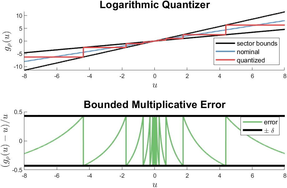
Figure 1: Logarithmic quantizer $(\rho=0.4)$ and error bound

The trajectories of a logarithmically quantized systems with $m=1$ are therefore contained in the class of scalar-$\Delta$ sector-bounded models:

$$x_{t+1} =\left[A+(1+\Delta)BK\right]x_{t} \forall\Delta\in[-\delta,\delta].$$ (9)

Theorem 2.1 of [4] proves that the state-feedback controller $u_{t}=Kx_{t}$ with $K\in\mathbb{R}^{1\times n}$ quadratically stabilizes (1) iff $u=Kx$ can quadratically stabilize (6).

For systems in which each input channel $u_{j}$ has a separate quantization density $(\rho_{j},\delta_{j})$, quadratic state-feedback stabilization of the quantized system will occur if [4, Theorem 3.2]:

$$\forall\Delta\in\textstyle\prod_{j=1}^{m}[-\delta_{j},\delta_{j}]$$

$$\qquad x_{t+1}=\left[A+B(I_{m}+\textrm{diag}(\Delta))K\right]x_{t}.$$ (10)

The work in [4] and [30] treat common stabilization of (9) as an $H_{\infty}$ optimization using the small-gain theorem for a sector-bounded uncertainty. The muli-input small-gain formulation in (10) is posed solved using a conservative multi-block S-Lemma.

3.3 Combined Superstability and Input-Quantization

We can apply extended superstabilization method Section 2.2 towards the control of input-quantized systems, as represented by the sector-bounded model class in (10).

Theorem 3.2.

A logarithmically quantized system in (6) is extended superstablized by a controller $u=Kx$ if there exists a $v\in\mathbb{R}_{>0}^{n},\ S\in\mathbb{R}^{m\times n},M\in\mathbb{R}^{n\times n}$ with $Y=\textrm{diag}(v)$

$$\forall i\in 1..n$$

$$\qquad\textstyle\sum_{j=1}^{n}M_{ij}<v_{i}$$ (11a)

$$\forall\Delta\in\textstyle\prod_{j=1}^{m}[-\delta_{j},\delta_{j}]$$

$$\textstyle-M\leq AY+B(I_{m}+\textrm{diag}(\Delta))S\leq M.$$ (11b)

The recovered controller is $K=SY^{-1}.$

Proof.

In the case where $\Delta=0$, then the quantized program (11) is equivalent to the unquantized program (3). We can apply Proposition 3.1 to generate a sector-bound description of quantization, together with separate input channel quantization based on Equation (10) regarding the multiplicative perturbations $\Delta$. The linear inequality constraints (11) are convex, such that a common $M$ is a worst-case certificate over the all possible closed-loop matrices $AY+B(I_{m}+\textrm{diag}(\Delta))S\leq M$. Such a certificate ensures extended superstability of all systems in (9). ∎

Corollary 1.

We can enumerate the convex constraint (11) over the vertices of the hypercube formed by $\delta$, producing the equivalent statement of

$$\forall\gamma\in\textstyle\prod_{j=1}^{m}\{-\delta_{j},\delta_{j}\}$$

$$\textstyle-M\leq AY+B(I_{m}+\textrm{diag}(\gamma))S\leq M.$$ (12)

Corollary 2.

An equivalent formulation to (11) with respect to sign-enumeration in (2) and substitution $\beta=1+\gamma$ is the following LP in $n2^{n+m}$ constraints:

$$\forall i\in 1..n,\ \alpha\in\{-1,1\}^{n},\ \beta\in\textstyle\prod_{j=1}^{m}\{1-\delta_{j},1+\delta_{j}\}:$$

$$\quad\textstyle\sum_{j=1}^{n}\alpha_{j}\left(A_{ij}v_{j}+\sum_{k=1}^{m}\beta_{k}B_{ik}S_{kj}\right)<v_{i}.$$ (13)

Proposition 3.3.

A controller $K$ that is feasible for quantization $\delta\in\mathbb{R}_{\geq 0}^{m}$ in (13) will also be feasible for every $\delta^{\prime}\in\mathbb{R}_{\geq 0}^{m}$ with $\delta^{\prime}\leq\delta$.

4 Quantized DDC

This section will outline DDC DDC approach towards quantized superstability.

Given data in $\mathcal{D}$, let $\mathcal{P}$ in (4) be the polytopic consistency of plants $(A,B)$ in agreement with $\mathcal{D}$.

Our task is to solve the following problem:

Problem 4.1.

Find a state-feedback controller $u=Kx$ such that the quantized system (9) is (extended) superstable for all $(A,B)\in\mathcal{P}$.

4.1 Consistency Polytope Representation

Let us define $\mathbf{X},\mathbf{U},\mathbf{p},\mathbf{q}$ as the following concatenations of data in $\mathcal{D}$:

$$\mathbf{X} =\begin{bmatrix}\hat{x}_{1};&\hat{x}_{2};&\ldots&\hat{x}_{N_{s}}\end{bmatrix}$$ (14a)

$$\mathbf{U} =\begin{bmatrix}\hat{u}_{1};&\hat{u}_{2};&\ldots&\hat{u}_{N_{s}}\end{bmatrix}$$ (14b)

$$\mathbf{p} =\begin{bmatrix}p_{1};&p_{2};&\ldots&p_{N_{s}}\end{bmatrix}$$ (14c)

$$\mathbf{q} =\begin{bmatrix}q_{1};&q_{2};&\ldots&q_{N_{s}}\end{bmatrix}.$$ (14d)

The data-consistency polytope in (4) may be represented using the data matrices in (14) as

$$G_{\mathcal{D}} =\begin{bmatrix}-\mathbf{X}^{T}\otimes I_{n}&-\mathbf{U}^{T}\otimes I_{n}\\ \mathbf{X}^{T}\otimes I_{n}&\mathbf{U}^{T}\otimes I_{n}\end{bmatrix}$$

$$h_{\mathcal{D}} =\begin{bmatrix}-\mathbf{p};&\mathbf{q}\end{bmatrix}$$ (15)

$$\mathcal{P} =\{(A,B)\mid G_{\mathcal{D}}[\textrm{vec}(A);\textrm{vec}(B)]\leq h_{\mathcal{D}}\},$$

using the Kronecker identity $\textrm{vec}(PXQ)=(Q^{T}\otimes P)\textrm{vec}(X)$ for matrices $(P,X,Q)$ of compatible dimensions. We will denote $L\leq 2nN_{s}$ as the number of faces in (15) ($h_{\mathcal{D}}\in\mathbb{R}^{1\times L}$). The number of faces $L$ can be reduced from $2nN_{s}$ by pruning redundant constraints from $\mathcal{P}$ [36] through iterative LPs.

4.2 Sign-Based Approach

The sign-based program in (13) in the DDC case can be considered as a finite-dimensional robust LP:

$$\forall i\in 1..n,\ \alpha\in\{-1,1\}^{n},\ \beta\in\textstyle\prod_{j=1}^{m}\{1-\delta_{j},1+\delta_{j}\}:$$ (16)

$$\quad\textstyle\sum_{j=1}^{n}\alpha_{j}\left(A_{ij}v_{j}+\sum_{k=1}\beta_{k}B_{ik}S_{kj}\right)<v_{i},\ \forall(A,B)\in\mathcal{P}.$$

Program (16) features a total of $n2^{n+m}$ strict robust inequalities. We will add a stability tolerance $\eta>0$ in order to modify the comparator and right-hand side of (16) into a nonstrict inequality $\leq v_{i}-\eta$. Each nonstrict robust inequality in $\alpha,\beta$ may be formulated as a polytope:

$$G_{\alpha\beta} =\begin{bmatrix}(\textrm{diag}(v)\alpha)^{T}\otimes I_{n}&(\textrm{diag}(\beta)S\alpha)^{T}\otimes I_{n}\end{bmatrix}$$

$$h_{\alpha\beta} =v-\eta\mathbf{1}$$ (17)

$$\mathcal{P}_{\alpha\beta} =\{(A,B)\mid G_{\alpha\beta}[\textrm{vec}(A);\textrm{vec}(B)]\leq h_{\alpha\beta}\}.$$

We will enforce containment of $\mathcal{P}$ in each $\mathcal{P}_{\alpha\beta}$ using the Extended Farkas Lemma:

Lemma 4.2 (Extended Farkas Lemma [37, 38]).

Let $P_{1}=\{x\mid G_{1}x\leq h_{1}\}$ and $P_{2}=\{x\mid G_{2}x\leq h_{2}\}$ be a pair of polytopes with $G_{1}\in\mathbb{R}^{m\times n}$ and $G_{2}\in\mathbb{R}^{p\times n}$. Then $P_{1}\subseteq P_{2}$ if and only if there exists a matrix $Z\in\mathbb{R}^{p\times m}_{\geq 0}$ such that,

$$ZG_{1} =G_{2}, Zh_{1}\leq h_{2}.$$ (18)

Remark 1.

The Extended Farkas Lemma is a particular instance of a robust counterpart [39] when certifying validity of a system of linear inequalities over polytopic uncertainty.

A sign-based program to solve Problem 4.1 is:

$$\operatorname*{find}_{v,S,Z}\quad \forall\alpha\in\{-1,1\}^{n},\ \beta\in\textstyle\prod_{j=1}^{m}\{1-\delta_{j},1+\delta_{j}\}:$$ (19a)

$$\qquad Z_{\alpha\beta}G_{\mathcal{D}}=G_{\alpha\beta},\quad Z_{\alpha\beta}h_{\mathcal{D}}\leq h_{\alpha\beta}$$ (19b)

$$\qquad Z_{\alpha\beta}\in\mathbb{R}_{\geq 0}^{n\times L}$$ (19c)

$$v-\eta\mathbf{1}_{n}\in\mathbb{R}_{\geq 0}^{n},\ S\in\mathbb{R}^{n\times m}.$$ (19d)

4.3 Lifted Approach

We can solve Problem 4.1 by posing (11) as an infinite-dimensional LP in terms of a function $M:\mathcal{P}\rightarrow\mathbb{R}^{n\times n}$.

Theorem 4.3.

A state-feedback controller $u=Kx$ will solve Problem 4.1 if the following infinite-dimensional LP has a feasible solution with $v\in\mathbb{R}_{>0}^{n},\ S\in\mathbb{R}^{m\times n},M:\mathcal{P}\rightarrow\mathbb{R}^{n\times n}$ with $Y=\textrm{diag}(v)$

$$\forall i\in 1..n$$

$$\qquad\textstyle\sum_{j=1}^{n}M_{ij}(A,B)<v_{i}$$ (20a)

$$\forall\beta\in\textstyle\prod_{j=1}^{m}\{1-\delta_{j},1+\delta_{j}\}$$

$$\textstyle-M(A,B)\leq AY+B(\textrm{diag}(\beta))S\leq M(A,B).$$ (20b)

Proof.

Each plant $(A,B)\in\mathcal{P}$ has a certificate of extended superstabilizability $(v,M(A,B))$ by Theorem 3.2. If (20) is feasible, then all plants in $\mathcal{P}$ simultaneously extended superstabilized by a common $K=SY^{-1}$ . ∎

Remark 2.

The function $M(A,B)$ may be treated as an adjustable decision variable given the a-priori unknown $(A,B)\in\mathcal{P}$ [40].

The infinite-dimensional LP in (20) must be truncated into a finite-dimensional convex program in order to admit computationally tractable formulations. One method to perform this truncation is to restrict $M(A,B)$ to an affine function by defining $M^{0},M^{A}_{ij},M^{B}_{ik}\in\mathbb{R}^{n\times n}$ to form

$$M(A,B) =\textstyle M^{0}+\sum_{ij}M^{A}_{ij}A_{ij}+\sum_{ik}M^{B}_{ik}B_{ik},$$ (21)

We can define the quantities $\mathbf{m}=(m^{0},m^{a},m^{b})$

$$m^{0} =\textrm{vec}(M^{0})$$ (22a)

$$m^{a} =\begin{bmatrix}\textrm{vec}(M^{A}_{11}),&\textrm{vec}(M^{A}_{21}),&\ldots,&\textrm{vec}(M^{A}_{nn})\end{bmatrix}$$ (22b)

$$m^{b} =\begin{bmatrix}\textrm{vec}(M^{B}_{11}),&\textrm{vec}(M^{B}_{21}),&\ldots,&\textrm{vec}(M^{B}_{nm})\end{bmatrix}.$$ (22c)

in order to obtain a vectorized expression for (21) with

$$\textrm{vec}(M(A,B)) =m^{0}+m^{a}\textrm{vec}(A)+m^{b}\textrm{vec}(B).$$ (23)

The row-sums of $$M$$ can be expressed as

$$\textrm{vec}(M(A,B)\mathbf{1}_{n}) =(\mathbf{1}_{n}^{T}\otimes I_{n})(m^{0}+m^{a}\textrm{vec}(A))$$ (24)

$$\qquad+(\mathbf{1}_{n}^{T}\otimes I_{n})(m^{b}\textrm{vec}(B)).$$

The constraint in (20a) with stability factor $\eta>0$ can be reformulated as membership in the following polytope $\mathcal{P}_{M}$:

$$G_{M} =(\mathbf{1}_{n}^{T}\otimes I_{n})\begin{bmatrix}m^{a},&m^{b}\end{bmatrix}$$

$$h_{M} =[v-\eta-(\mathbf{1}_{n}^{T}\otimes I_{n})m^{0}]$$ (25)

$$\mathcal{P}_{M} =\{(A,B)\mid G_{M}[\textrm{vec}(A);\textrm{vec}(B)]\leq h_{M}\}.$$

The polytopic constraint region in (20b) for each $\beta\in\textstyle\prod_{j=1}^{m}\{1-\delta_{j},1+\delta_{j}\}$ is

$$G_{\beta}^{s} =\begin{bmatrix}-m^{a}-\textrm{diag}(v)^{T}\otimes I_{n}&-m^{b}-(\textrm{diag}(\beta)S)^{T}\otimes I_{n}\\ -m^{a}+\textrm{diag}(v)^{T}\otimes I_{n}&-m^{b}+(\textrm{diag}(\beta)S)^{T}\otimes I_{n}\end{bmatrix}$$

$$h_{\beta} =\begin{bmatrix}m^{0};&m^{0}\end{bmatrix}$$ (26)

$$\mathcal{P}_{\beta} =\{(A,B)\mid G_{\beta}[\textrm{vec}(A);\textrm{vec}(B)]\leq h_{\beta}\}.$$

The affine restriction of $M$ in (21) results in AARC AARC program for (20):

$$\operatorname*{find}_{v,S,Z,\mathbf{m}}\quad \forall\beta\in\textstyle\prod_{j=1}^{m}\{1-\delta_{j},1+\delta_{j}\}:$$ (27a)

$$Z_{\beta}G_{\mathcal{D}}=G_{\beta},\quad Z_{\beta}h_{\mathcal{D}}\leq h_{\beta}$$ (27b)

$$Z_{\beta}\in\mathbb{R}_{\geq 0}^{2n^{2}\times L}$$ (27c)

$$Z_{M}G_{\mathcal{D}}=G_{M},\quad Z_{M}h_{\mathcal{D}}\leq h_{M}$$ (27d)

$$Z_{M}\in\mathbb{R}^{n\times L}_{\geq 0}$$ (27e)

$$m^{0}\in\mathbb{R}^{n^{2}\times 1},\ m^{A}\in\mathbb{R}^{n^{2}\times n^{2}}$$ (27f)

$$m^{B}\in\mathbb{R}^{n^{2}\times nm}$$ (27g)

$$v-\eta\mathbf{1}_{n}\in\mathbb{R}_{\geq 0}^{n},\ S\in\mathbb{R}^{n\times m}.$$ (27h)

4.4 Computational Complexity

We will quantify the computational complexity (19) and (27) based on the number of robust inequalities (for (16) and (20)), scalar variables $(v,S,Z,\mathbf{m})$, slack variables/constraints introduced in reformulations of scalar inequality constraints (e.g., $v-\eta\mathbf{1}_{n}\in\mathbb{R}^{n}_{\geq 0}\mapsto q\in\mathbb{R}^{n}_{\geq 0},\ v-\eta\mathbf{1}_{n}=q$), scalar inequality constraints $(\in\mathbb{R}_{\geq 0})$, and scalar equality constraints. These counts (up to the highest order terms to save space) are listed in Table 1.

Table 1: Comparison between LPs (19) and (27)

	sign-based (19)	AARC (27)
robust ineq.	$n2^{n+m}$	$n+n^{2}2^{m+1}$
scalar vars.	$n(m+1+2^{n+m}L)$	$n(m+1)+n^{2}(1+nm+n^{2})$
		$\quad+n^{2}L2^{m+1}$
slack vars.	$n+2^{n+m+1}n^{2}$	$n(1+2^{m+1})$
eq. cons.	$n^{2}(n+m)2^{n+m}+n$	$(2^{m+1}n^{2}+n)(n+m)+n$
ineq. cons.	$2^{n+m}(n+nL)+n$	$n(L+2)+n^{2}(L+1)2^{m+1}$

Note how $n$ appears exponentially in the sign-based scheme (19), while $n$ enters only polynomially for quantities in the AARC (27).

Given that the running-time of an Interior Point Method for $N$-variable LPs up $\gamma$-optimality is approximately $O(N^{\omega+0.5}\lvert\log(1/\gamma)\rvert)$ (with matrix multiplication constant $\omega$) [41], the AARC is more computationally efficient than the sign-based scheme as $n$ increases.

5 Numerical Examples

MATLAB (2021a) code to execute all examples is publicly available . The convex optimization problems (19) and (27) are modeled in YALMIP [42] (including the robust programming module [43] with option ‘lplp.duality’) and solved in Mosek 9.2 [44].

5.1 3-state 2-input

The first example will involve superstabilization of the following system 3-state 2-input discrete-time linear system:

$$A =\begin{bmatrix}-0.1300&-0.3974&0.2030\\ -0.3974&-0.5000&0.2990\\ 0.2030&0.2990&-0.5262\end{bmatrix},$$ (28a)

$$B =\begin{bmatrix}0.2179&1.2300\\ 0.3592&0\\ -1.1553&0\end{bmatrix}.$$ (28b)

System (28) is open-loop unstable with eigenvalues of $[-1.0185,-0.2613,0.1236].$

We collect $T=100$ input-state-transition observations of system (28) to form $\mathcal{D}$. The transition observations are quantized according to the following partition with 9 bins:

$$(-\infty,-4]\cup[-4,-3]\cup[-3,-2]\ldots[3,4]\cup[4,\infty).$$ (29)

Superstabilization $(v=\mathbf{1}_{3})$ is performed by solving the sign-based scheme in (16). An objective is added to minimize $\lambda\in\mathbb{R}$ such that $\forall i:\sum_{j}M_{ij}\leq\lambda$, in which $\lambda<1$ indicates a successful worst-case superstabilization under input and data quantization.

Figure 2 plots worst-case optimal values of $\lambda$ as a function of the quantization density $\rho$, in which $\rho$ is the same for all inputs. The $T=60$ data preserves the first 60 elements of the 100 observations in $\mathcal{D}$ (with a similar process for $T=80$). Gain values for the ground truth (model-based case when (28) is known) are presented as a comparison. We note that $\rho\rightarrow 1$ results in $\delta\rightarrow 0$ by (7), for which the (limiting) quantization law at $\rho=1$ is $g_{\rho=1}(u)=u$.

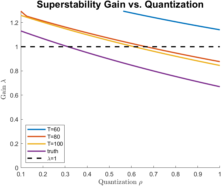
Figure 2: Peak-to-peak gain $(\lambda)$ vs. quantization density $(\rho)$

Table 2 lists the minimal feasible $\rho$ (up to four decimal places) such that the sign-based formulation in (16) returns a feasible superstabilizing (SS) or extended superstabilizing (ESS) controller. The symbol $\varnothing$ indicates primal infeasiblility of the LP for all $\rho\leq 1$.

Table 2: Minimal $\rho$ with sign-based of (28)

$T$	60	80	100	Truth
SS	$\varnothing$	0.6727	0.6182	0.3182
ESS	0.9397	0.3494	0.2081	0.1422

Table 3 lists the minimal $\rho$ for AARC-based quantized superstabilization. There is no difference between the ground-truth values in Tables 2 and 3, because the underlying finite-dimensional LPs with nonrobust inequality constraints are equivalent.

Table 3: Minimal $\rho$ with AARC stabilization of (28)

$T$	60	80	100	Truth
SS	$\varnothing$	$\varnothing$	0.9500	0.3182
ESS	$\varnothing$	$\varnothing$	0.7723	0.1422

5.2 5-state 3-input

The second example performs extended superstabilization over the following system with 5 states and 3 inputs:

$$A =(1/5)[\min(i/j,j/i)]_{ij}+(1/2)I_{5},$$ (30a)

$$B =[I_{3};\mathbf{0}_{2\times 3}].$$ (30b)

System (30) is open-loop unstable with purely real eigenvalues of $[1.0633,0.6507,0.5502,0.5046,0.4812]$. The nominal system in (30) can be extended-superstabilized until $\rho=0.2245$.

The $T=350$ state-input collected transitions of (30) are quantized according to the following partition with 26 bins:

$$(-\infty,-6]\cup[-6,-5.5]\cup[-5.5,-5]\ldots[5.5,6]\cup[6,\infty).$$ (31)

The polytope in (4) has $2nT=3500$ faces in $n(n+m)=40$ dimensions, of which $185$ of these faces are nonredundant.

We successfully solve the data-driven common-extended-superstabilizing AARC program in (27) at $\rho=0.8$ to acquire a feasible controller with parameters

$$K =-\begin{bmatrix}0.6434&0.0943&0.0785&0.0609&0.0330\\ 0.0965&0.6513&0.1409&0.0899&0.0842\\ 0.0650&0.1392&0.6528&0.1463&0.1183\\ \end{bmatrix}$$

$$v =\begin{bmatrix}0.0137,&0.0069&0.0058&0.0289&0.0289\end{bmatrix}.$$ (32)

6 Conclusion

This paper presented a method to perform superstabilizing control of linear systems under state-transition data quantization and actuated-input quantization. The generated sign-based finite-dimensional LP and lifted infinite-dimensional LPs are nonconservative with respect to the common superstabilization task. This infinite-dimensional LP has a number of constraints that is polynomial in the number of states $n$ and exponential in the number of inputs $m$. AARC AARC was employed to truncate the infinite-dimensional LP, in order to gain tractability at the expense of conservatism.

The logarithmic-quantization approach laid out in this paper involves an infinite number of quantization levels. Future work includes adapting the adaptive finite-level quantizing method of [5] for DDC-superstabilization. Other investigations aim to decrease the computational impact of the presented scheme by formulating nonconservative LP formulations that scale in a polynomial manner with $m$ rather than in an exponential manner, by reducing the conservatism of the AARC truncation by allowing $M$ to be polynomial (using sum-of-squares certificates of nonnegativity), and by formulating control laws in the setting where $(\hat{x},\hat{u})$ are also data-quantized (resulting in an Error-in-Variables model [45] addressable by polynomial optimization [17]).

References

- [1] R. W. Brockett and D. Liberzon, “Quantized feedback stabilization of linear systems,” IEEE transactions on Automatic Control, vol. 45, no. 7, pp. 1279–1289, 2000.
- [2] N. Elia and S. K. Mitter, “Stabilization of linear systems with limited information,” IEEE transactions on Automatic Control, vol. 46, no. 9, pp. 1384–1400, 2001.
- [3] D. Nesic and D. Liberzon, “A unified framework for design and analysis of networked and quantized control systems,” IEEE Transactions on Automatic Control, vol. 54, no. 4, pp. 732–747, 2009.
- [4] M. Fu and L. Xie, “The sector bound approach to quantized feedback control,” IEEE Transactions on Automatic Control, vol. 50, no. 11, pp. 1698–1711, 2005.
- [5] ——, “Finite-level quantized feedback control for linear systems,” IEEE Transactions on Automatic Control, vol. 54, no. 5, pp. 1165–1170, 2009.
- [6] J. Zhou and C. Wen, “Adaptive backstepping control of uncertain nonlinear systems with input quantization,” in 52nd IEEE conference on decision and control. IEEE, 2013, pp. 5571–5576.
- [7] Z.-S. Hou and Z. Wang, “From model-based control to data-driven control: Survey, classification and perspective,” Information Sciences, vol. 235, pp. 3–35, 2013, data-based Control, Decision, Scheduling and Fault Diagnostics.
- [8] S. Formentin, K. Van Heusden, and A. Karimi, “A comparison of model-based and data-driven controller tuning,” International Journal of Adaptive Control and Signal Processing, vol. 28, no. 10, pp. 882–897, 2014.
- [9] Z. Hou, H. Gao, and F. L. Lewis, “Data-Driven Control and Learning Systems,” IEEE Transactions on Industrial Electronics, vol. 64, no. 5, pp. 4070–4075, 2017.
- [10] Y. Cheng, M. Sznaier, and C. Lagoa, “Robust Superstabilizing Controller Design from Open-Loop Experimental Input/Output Data,” IFAC-PapersOnLine, vol. 48, no. 28, pp. 1337–1342, 2015.
- [11] J. Miller, T. Dai, M. Sznaier, and B. Shafai, “Data-Driven Control of Positive Linear Systems using Linear Programming,” in 62nd IEEE Conference on Decision and Control, 2023.
- [12] H. J. van Waarde, M. K. Camlibel, and M. Mesbahi, “From Noisy Data to Feedback Controllers: Nonconservative Design via a Matrix S-Lemma,” IEEE Trans. Automat. Contr., 2020.
- [13] H. J. van Waarde, M. K. Camlibel, J. Eising, and H. L. Trentelman, “Quadratic matrix inequalities with applications to data-based control,” SIAM J Control Optim, vol. 61, no. 4, pp. 2251–2281, 2023.
- [14] J. Miller and M. Sznaier, “Data-Driven Gain Scheduling Control of Linear Parameter-Varying Systems using Quadratic Matrix Inequalities,” IEEE Control Systems Letters, vol. 7, pp. 835–840, 2022.
- [15] T. Dai and M. Sznaier, “A Semi-Algebraic Optimization Approach to Data-Driven Control of Continuous-Time Nonlinear Systems,” IEEE Control Systems Letters, vol. 5, no. 2, pp. 487–492, 2020.
- [16] T. Martin and F. Allgöwer, “Data-driven system analysis of nonlinear systems using polynomial approximation,” arXiv preprint arXiv:2108.11298, 2021.
- [17] J. Miller, T. Dai, and M. Sznaier, “Data-Driven Superstabilizing Control of Error-in-Variables Discrete-Time Linear Systems,” in 2022 61st IEEE Conference on Decision and Control (CDC), 2022, pp. 4924–4929.
- [18] J. Zheng, T. Dai, J. Miller, and M. Sznaier, “Robust data-driven safe control using density functions,” IEEE Control Systems Letters, 2023.
- [19] H. Hjalmarsson, M. Gevers, S. Gunnarsson, and O. Lequin, “Iterative Feedback Tuning: Theory and Applications,” IEEE control systems magazine, vol. 18, no. 4, pp. 26–41, 1998.
- [20] M. C. Campi, A. Lecchini, and S. M. Savaresi, “Virtual reference feedback tuning: a direct method for the design of feedback controllers,” Automatica, vol. 38, no. 8, pp. 1337–1346, 2002.
- [21] S. Savaresi and L. Del Re, “Non-iterative direct data-driven controller tuning for multivariable systems: theory and application,” IET control theory & applications, vol. 6, no. 9, pp. 1250–1257, 2012.
- [22] J. C. Willems, P. Rapisarda, I. Markovsky, and B. L. De Moor, “A note on persistency of excitation,” Systems & Control Letters, vol. 54, no. 4, pp. 325–329, 2005.
- [23] C. De Persis and P. Tesi, “Formulas for Data-Driven Control: Stabilization, Optimality, and Robustness,” IEEE Trans. Automat. Contr., vol. 65, no. 3, pp. 909–924, 2020.
- [24] J. Coulson, J. Lygeros, and F. Dörfler, “Data-Enabled Predictive Control: In the Shallows of the DeePC,” in 2019 18th European Control Conference (ECC), 2019, pp. 307–312.
- [25] J. Berberich, J. Köhler, M. A. Müller, and F. Allgöwer, “Data-Driven Model Predictive Control With Stability and Robustness Guarantees,” IEEE Trans. Automat. Contr., vol. 66, no. 4, pp. 1702–1717, 2021.
- [26] T. Dai and M. Sznaier, “A Moments Based Approach to Designing MIMO Data Driven Controllers for Switched Systems,” in 2018 IEEE Conference on Decision and Control (CDC), 2018, pp. 5652–5657.
- [27] A. Robey, H. Hu, L. Lindemann, H. Zhang, D. V. Dimarogonas, S. Tu, and N. Matni, “Learning control barrier functions from expert demonstrations,” in 2020 59th IEEE Conference on Decision and Control (CDC), 2020, pp. 3717–3724.
- [28] ——, “Learning control barrier functions from expert demonstrations,” in 2020 59th IEEE Conference on Decision and Control (CDC), 2020, pp. 3717–3724.
- [29] A. J. Thorpe, C. Neary, F. Djeumou, M. M. K. Oishi, and U. Topcu, “Physics-informed kernel embeddings: Integrating prior system knowledge with data-driven control,” 2023.
- [30] F. Zhao, X. Li, and K. You, “Data-driven control of unknown linear systems via quantized feedback,” in Learning for Dynamics and Control Conference. PMLR, 2022, pp. 467–479.
- [31] B. Polyak and M. Halpern, “Optimal design for discrete-time linear systems via new performance index,” International Journal of Adaptive Control and Signal Processing, vol. 15, no. 2, pp. 129–152, 2001.
- [32] B. T. Polyak and P. S. Shcherbakov, “Superstable Linear Control Systems. I. Analysis,” Automation and Remote Control, vol. 63, no. 8, pp. 1239–1254, 2002.
- [33] B. T. Polyak, “Extended superstability in control theory,” Automation and Remote Control, vol. 65, no. 4, pp. 567–576, 2004.
- [34] M. Yannakakis, “Expressing combinatorial optimization problems by Linear Programs,” Journal of Computer and System Sciences, vol. 43, no. 3, pp. 441–466, 1991.
- [35] M. Sznaier, R. Suárez, S. Miani, and J. Alvarez-Ramírez, “Optimal disturbance rejection and global stabilization of linear systems with saturating control,” IFAC Proceedings Volumes, vol. 29, no. 1, pp. 3550–3555, 1996, 13th World Congress of IFAC, 1996, San Francisco USA, 30 June - 5 July.
- [36] R. Caron, J. McDonald, and C. Ponic, “A degenerate extreme point strategy for the classification of linear constraints as redundant or necessary,” Journal of Optimization Theory and Applications, vol. 62, no. 2, pp. 225–237, 1989.
- [37] J.-C. Hennet, “Une extension du lemme de farkas et son application au problème de régulation linéaire sous contraintes,” C. R. Acad. Sciences, vol. 308, 01 1989.
- [38] D. Henrion, S. Tarbouriech, and V. Kučera, “Control of linear systems subject to input constraints: a polynomial approach. Part I. SISO plants,” in Proceedings of the 38th IEEE Conference on Decision and Control (Cat. No. 99CH36304), vol. 3, 1999, pp. 2774–2779.
- [39] A. Ben-Tal, L. El Ghaoui, and A. Nemirovski, Robust Optimization. Princeton university press, 2009, vol. 28.
- [40] İ. Yanıkoğlu, B. L. Gorissen, and D. den Hertog, “A survey of adjustable robust optimization,” European Journal of Operational Research, vol. 277, no. 3, pp. 799–813, 2019.
- [41] S. J. Wright, Primal-Dual Interior-Point Methods. SIAM, 1997.
- [42] J. Lofberg, “YALMIP : A toolbox for modeling and optimization in MATLAB,” in ICRA (IEEE Cat. No.04CH37508), 2004, pp. 284–289.
- [43] J. Löfberg, “Automatic robust convex programming,” Optimization methods and software, vol. 27, no. 1, pp. 115–129, 2012.
- [44] M. ApS, The MOSEK optimization toolbox for MATLAB manual. Version 9.2., 2020. [Online]. Available: https://docs.mosek.com/9.2/toolbox/index.html
- [45] T. Söderström, “Errors-in-variables methods in system identification,” Automatica, vol. 43, no. 6, pp. 939–958, 2007.