Simple Power-law model for generating correlated particles

Abstract

A search for the critical point of the strongly interacting matter by studying power-law fluctuations within the framework of intermittency is ongoing. In particular, experimental data on proton and pion production in heavy-ion collisions are analyzed in transverse momentum space. In this regard, a simple model with a power-law multi-particle correlations is introduced. The model can be used to study sensitivity to detect power-law correlated particles in the presence of various detector effects.

I Motivation

One of the goals of the high-energy heavy-ion physics is to locate the critical point (CP) in the phase diagram of the strongly interacting matter. Theoretical studies suggest a smooth crossover transition at small baryochemical potential $\mu_{B}$ and high temperature $T$ Aoki:2006we . At lower $T$ and larger $\mu_{B}$, a first-order phase transition is expected Asakawa:1989bq . The CP is a hypothetical end point of the first-order phase transition that has properties of the second-order phase transition.

In the vicinity of CP, fluctuations of the order parameter become self-similar Antoniou:2006zb , belonging to the 3D-Ising universality class. This can be detected by studying particles’ fluctuations in the transverse momentum, $p_{T}$, space within the framework of intermittency analysis by use of Scaled Factorial Moments (SFM). A search for such power-law fluctuations was proposed in Refs. Bialas:1985jb ; Bialas:1988wc ; Satz:1989vj ; Gupta:1990bi and experimental data on proton and pion multiplicity fluctuations have been analyzed in transverse momentum space Anticic:2009pe ; Anticic:2012xb ; Davis:2020fcy .

To study the sensitivity to detect power-law correlated particles in the presence of various detector effects, a simple, fast model that can generate particles with properties expected for the CP was developed and is presented below.

II Power-Law Model

The Power-Law Model generates events with momenta of a given number of particles with a given power-law correlation of their transverse momentum difference and/or a given number of uncorrelated particles while maintaining a given shape of single-particle inclusive $p_{T}$ distribution and a given multiplicity distribution. Results, events with list of particles with their momenta components, are stored in a text file and can be used for calculating SFM or undergo further processing (e.g. momentum smearing to mimic detector’s momentum resolution). The model is written in ANSI C with no external dependencies. It uses SFC64 sfc64 random number generator.

II.1 Power-law correlation

The model allows for generating groups of correlated particles (pairs, triplets, quadruplets, etc.). The correlations are introduced using the average, over particles in a group, pair transverse momentum difference $S$. For a given number of particles in a group $g$ that form $g_{\text{p}}=g(g-1)/2$ pairs, $S$ is defined as

$$S=\frac{1}{g_{\text{p}}}\sum\limits_{i=1}^{g}\sum\limits_{\begin{subarray}{c}j=1\\ j\neq i\end{subarray}}^{g}|\Delta\overrightarrow{p_{T}}|_{i,j}\,.$$ (1)

For a correlated pair, when $g=2$ and ${g_{\text{p}}=1}$, $S$ is equal to the difference of the two particles transverse momenta, $S=|\Delta\overrightarrow{p_{T}}|$.

The correlations are introduced by generating $S$ according to the power-law distribution:

$$\rho_{S}(S)=S^{-\phi}\,,$$ (2)

with a given exponent $0\leq\phi<1$. Due to scaling of power law, $S$ for sub-groups of $g$ particles follow the same distribution (e.g. quadruplet of particles correlated with $\phi$ consists of 4 triplets correlated with $\phi$ and 6 pairs also correlated with $\phi$).

II.2 Event multiplicity

Number of events, $N_{\text{events}}$, is one of the input (command-line) parameters. Processing will stop after reaching the requested value. Number of particles in each event is drawn from either a standard distribution (e.g Poisson with a given expected value) or a custom distribution supplied in a text file. Event multiplicity can also be set to a constant value.

II.3 Particles’ transverse momentum components

In order to generate transverse momentum components of each particle, the following parameters are used:

1. desired ratio of total number of correlated particles to all particles $r$ (default: 0.5),

2. power-law exponent $\phi$ (default: 0.8),

3. minimum and maximum value of the average pair momentum difference $S$ of correlated particles (default: $S_{\text{min}}=0.0$, $S_{\text{max}}=1.2$ GeV/c),

4. number of correlated particle in group $g$ (default: 2),

5. single-particle transverse momentum distribution $\rho_{p_{T}}(p_{T})$ (up to $p_{T}{}_{\text{max}}=1.5$ GeV/c) in a text file (default: $\rho_{p_{T}}(p_{T})=p_{T}exp(-6p_{T})$).

Uncorrelated particles are generated as long, as generating a correlated group would still not exceed the ratio $r$. Then, a correlated group if generated.

II.3.1 Uncorrelated particles

Generating uncorrelated particle’s transverse momentum components takes following steps:

1. draw $p_{T}$ form the supplied transverse momentum distribution $\rho_{p_{T}}$,

2. draw azimuthal angle $\varphi$ from a uniform distribution [$0,2\pi$),

3. calculate the components, as $p_{x}=p_{T}cos(\varphi)$ and $p_{y}=p_{T}sin(\varphi)$.

II.3.2 Correlated particles

Before generating the first correlated group, the total number of correlated particles is estimated, as

$$n_{\text{c}}=N_{\text{events}}\cdot\langle N\rangle\cdot r\,,$$

where $\langle N\rangle$ is the mean value of the requested multiplicity distribution. Total number of correlated groups to be generated is $n_{\text{g}}=n_{\text{c}}/g$.

Then, an array of $n_{\text{g}}$ values of $S$ following the power-law distribution $\rho_{S}$ from Eq. 2 is generated and sorted in ascending order. Each value is calculated using the inverse transform sampling method (with additional constraints on minimum and maximum values of $S$) as

$$S_{i}=\left[(S_{\text{min}})^{1-\phi}+\left((S_{\text{max}})^{1-\phi}-(S_{\text{min}})^{1-\phi}\right)R_{i}\right]^{\frac{1}{1-\phi}}\,,$$

where $i=1\ldots n_{\text{g}}$ and $R_{i}$ are random numbers from a uniform distribution $[0,1)$.

Also, a histogram $H$ of each correlated particle’s transverse momentum is created by randomly drawing $n_{\text{c}}$ values of $p_{T}$ from $\rho_{p_{T}}$.

In the $p_{x}-p_{y}$ plane, each correlated particle in a group, is evenly positioned on a circle with diameter $S$, centered at their average $p_{T}$. For each group a next value from the array of $S$ values is used. In combination with the maximum value of $p_{T}$, 1.5 GeV/c, it determines available range of values of single particle $p_{T}$. Next, a 1D probability distribution of available $p_{T}$ values from histogram $H$ is constructed. It is then used to draw average $p_{T}$ of particles in group.

Having the center (average $p_{T}$) and the diameter ($S$) of the circle in $p_{x}-p_{y}$ plane, particles are placed evenly starting at a random position. Then, components of their transverse momenta are calculated and stored.

As a last step, histogram $H$ is updated by removing obtained values of $p_{T}$.

II.4 Particles’ longitudinal momentum components

Both correlated and uncorrelated particles’ longitudinal momentum components $p_{z}$ are calculated independently from $p_{T}$ from a center-of-mass rapidity distribution. The following parameters are used:

1. minimum and maximum value of the center-of-mass rapidity (default: $y_{\text{min}}^{\text{CMS}}=-0.75$, $y_{\text{max}}^{\text{CMS}}=0.75$),

2. mass of particles $m$ (default: 0.938 GeV),

3. rapidity of the center-of-mass in laboratory frame (default: $y_{\text{cms}}^{\text{LAB}}=2.88$).

The center-of-mass rapidity distribution is assumed to be uniform in a given range and one value $y^{\text{CMS}}$ is chosen at random. Using a given particle mass and generated $p_{T}$, transverse mass is calculated as

$$m_{T}=\sqrt{(p_{T})^{2}+m^{2}}\,.$$

Knowing rapidity of the center-of-mass in laboratory frame and transverse mass allows to calculate $p_{z}$:

$$p_{z}=m_{T}\cdot sinh(y^{\text{CMS}}+y_{\text{cms}}^{\text{LAB}})\,.$$

II.5 Model performance

The key feature of the model is introducing a power-law correlation of particles while preserving a given single-particle transverse momentum distribution. To test it, 10000 events with different settings have been generated and the relevant distributions are shown in Fig. 1. For $\phi=0.8$ and $\phi=0.5$ the model generates power-law distributions close to the ones requested (bottom). Also, for the two requested transverse momentum distributions, generated data follow them closely (top).

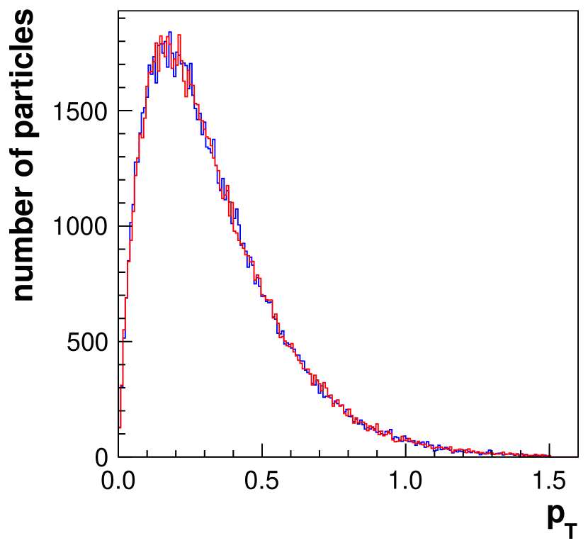
(a) $\rho_{p_{T}}(p_{T})=p_{T}exp(-6p_{T})$,
$\phi=0.8$, $r=0.5$, $g=2$, $N=2$

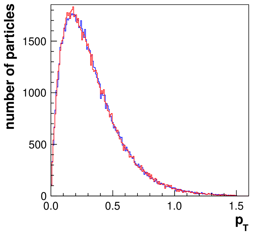
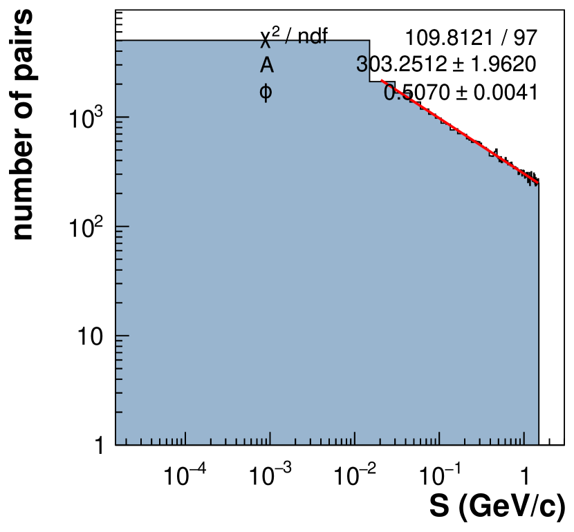
(b) $\rho_{p_{T}}(p_{T})=p_{T}exp(-6p_{T})$,
$\phi=0.5$, $r=0.5$, $g=2$, $N=2$

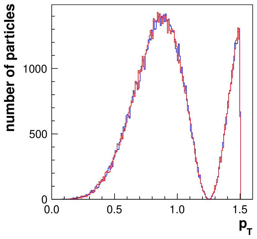
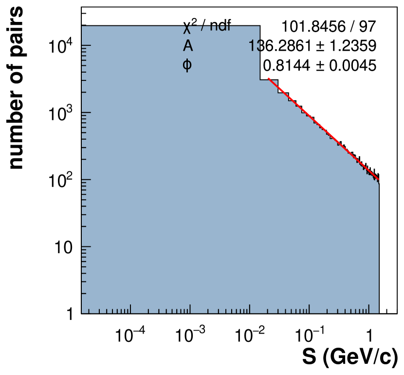
(c) $\rho_{p_{T}}(p_{T})=sin^{2}(2(p_{T})^{2})$,
$\phi=0.8$, $r=0.5$, $g=2$, $N=2$

Figure 1: Transverse momentum (top) and $S$ (bottom) distributions for 10000 events generated with different model parameters. Transverse momentum distributions are plotted separately for uncorrelated (blue) and correlated (red) particles. The $S$ distribution is fitted with $f(S)=A\cdot S^{-\phi}$ and presented in log-log scale to reveal the power-law shape.

Generating these data sets took approximately 200ms each.

II.6 Scaled Factorial Moments for the model data

The main purpose of the model is to study SFM, which is used within intermittency analysis as a tool for locating the CP. Therefore it must generate particles with properties expected for the CP. One of the properties, power-law correlation is explicitly built-in in the model. It would result in a power-law dependence of SFM of the order $q$ with respect to the number of $p_{x}$–$p_{y}$ cells $M^{2}$:

$$F_{q}(M)\propto(M^{2})^{\phi_{q}}\,.$$

Another feature of SFM in the vicinity of the CP is a linear relation between exponents (intermittency indices) $\phi_{q}$. To test it with the model, 10000 events each containing $N=6$, all correlated particles ($r=1$, $g=6$, $\phi=0.8$) have been generated. Then, SFM up to $q=6$ order were calculated and fitted with a power law. Results are shown in the left panel of Fig. 2. The obtained exponents $\phi_{2},\dots,\phi_{6}$ are presented in the right panel. Clearly they do exhibit expected linearity.

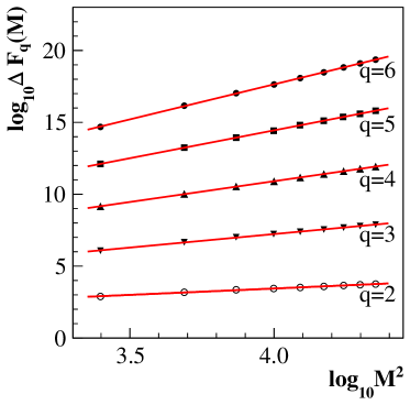
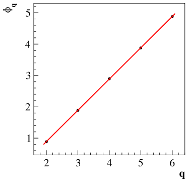
Figure 2: SFM of the orders from $q=2$ to $q=6$ (left) and power-law exponents $\phi_{2},\dots,\phi_{6}$ obtained from their fits (right) for 10000 events with 6 correlated particles each, generated with the model.

III Summary and outlook

This work is motivated by experimental searches for the critical point of the strongly interacting matter in heavy-ion collisions. A model introducing a power-law correlation predicted in the vicinity of the CP was presented. The expected scaling behavior of $F_{q}(M)$ in $M^{2}$ as well as a linear relation of obtained intermittency indices is observed. Introducing correlations between particles does not affect transverse momentum and multiplicity distributions.

The model can be used to study the impact of detector effects (e.g. acceptance, efficiency, resolution, etc.) on the behavior of the scaled factorial moments.

- (1) Y. Aoki, G. Endrodi, Z. Fodor, S. Katz, and K. Szabo, “The Order of the quantum chromodynamics transition predicted by the standard model of particle physics,” Nature, vol. 443, pp. 675–678, 2006.
- (2) M. Asakawa and K. Yazaki, “Chiral Restoration at Finite Density and Temperature,” Nucl. Phys. A, vol. 504, pp. 668–684, 1989.
- (3) N. G. Antoniou, F. K. Diakonos, A. S. Kapoyannis, and K. S. Kousouris, “Critical opalescence in baryonic QCD matter,” Phys. Rev. Lett., vol. 97, p. 032002, 2006.
- (4) A. Bialas and R. B. Peschanski, “Moments of Rapidity Distributions as a Measure of Short Range Fluctuations in High-Energy Collisions,” Nucl. Phys. B, vol. 273, pp. 703–718, 1986.
- (5) A. Bialas and R. B. Peschanski, “Intermittency in Multiparticle Production at High-Energy,” Nucl. Phys. B, vol. 308, pp. 857–867, 1988.
- (6) H. Satz, “Intermittency and Critical Behavior,” Nucl. Phys. B, vol. 326, pp. 613–618, 1989.
- (7) S. Gupta, P. La Cock, and H. Satz, “The Search for intermittency in the finite size Ising model,” Nucl. Phys. B, vol. 362, pp. 583–598, 1991.
- (8) T. Anticic et al., “Search for the QCD critical point in nuclear collisions at the CERN SPS,” Phys. Rev. C, vol. 81, p. 064907, 2010.
- (9) T. Anticic et al., “Critical fluctuations of the proton density in A+A collisions at 158 GeV,” Eur. Phys. J. C, vol. 75, no. 12, p. 587, 2015.
- (10) N. Davis, “Searching for the Critical Point of Strongly Interacting Matter in Nucleus–Nucleus Collisions at CERN SPS,” Acta Phys. Polon. Supp., vol. 13, no. 4, pp. 637–643, 2020.
- (11) http://pracrand.sourceforge.net.