A Neural-Guided Dynamic Symbolic Network for Exploring Mathematical Expressions from Data

Abstract

Symbolic regression (SR) is a powerful technique for discovering the underlying mathematical expressions from observed data. Inspired by the success of deep learning, recent efforts have focused on two categories for SR methods. One is using a neural network or genetic programming to search the expression tree directly. Although this has shown promising results, the large search space poses difficulties in learning constant factors and processing high-dimensional problems. Another approach is leveraging a transformer-based model training on synthetic data and offers advantages in inference speed. However, this method is limited to fixed small numbers of dimensions and may encounter inference problems when given data is out-of-distribution compared to the synthetic data. In this work, we propose DySymNet, a novel neural-guided Dynamic Symbolic Network for SR. Instead of searching for expressions within a large search space, we explore DySymNet with various structures and optimize them to identify expressions that better-fitting the data. With a topology structure like neural networks, DySymNet not only tackles the challenge of high-dimensional problems but also proves effective in optimizing constants. Based on extensive numerical experiments using low-dimensional public standard benchmarks and the well-known SRBench with more variables, our method achieves state-of-the-art performance in terms of fitting accuracy and robustness to noise.

1 Introduction

Numerous phenomena in the natural world, such as physical laws, can be precisely described using mathematical expressions. Symbolic regression (SR) is an effective machine-learning technique that involves discovering mathematical expressions that describe a dataset with accuracy. Unlike polynomial or neural network-based regression, SR aims to unveil the fundamental principles underlying the data generation process. This method is analogous to how physicists use explicit mathematical models to explain physical phenomena. For instance, Isaac Newton’s laws of motion provided a mathematical framework for describing object motion, while Albert Einstein’s theory of relativity introduced new equations to explain the behavior of objects in motion. More specifically, given a dataset $(X,y)$, where each feature $X_{i}\in\mathbb{R}^{n}$ and target $y_{i}\in\mathbb{R}$, the goal of SR is to identify a function $f$ (i.e., $y\approx f(X)$ $:\mathbb{R}^{n}\rightarrow\mathbb{R}$) that best fits the dataset, where the functional form of $f$ is a short closed-form mathematical expression.

SR is a challenging task because the search space of expressions grows exponentially with the length of the expression, while the position and value of numeric further exacerbate its difficulty. The traditional SR methods mainly involve heuristic search methods based on genetic programming (GP) (Forrest, 1993; Koza, 1994; Schmidt and Lipson, 2009; Staelens et al., 2013; Arnaldo et al., 2015; Bładek and Krawiec, 2019). They represent the expression as a binary tree and find high-fitness solutions through iterative evolutions in the large functional search space. While GP-based SR methods have the capability to solve nonlinear problems, they often yield complex expressions and are computationally expensive. Furthermore, these methods are known to exhibit high sensitivity to hyperparameters, which can complicate the optimization process. A more recent line of research has made use of the neural network to tackle the aforementioned shortcomings. Martius and Lampert (2016) proposed an equation learner (EQL), a fully-connected network where elementary functions are used as activation functions. They try to constrain the search space by optimizing a pre-defined network. The limitation of EQL is that the pre-defined architecture of the network limits the complexity of the predicted expression and is not flexible for different specific problems. Recently, reinforcement learning (RL)-based methods (Petersen et al., ; Mundhenk et al., 2021) for SR have shown promising results. They directly search expressions in the large functional space guided by RL. Although it is effective in dealing with low-dimensional problems without constants, they face difficulties in handling high-dimensional problems and constant optimization due to the large search space. Inspired by the success of large-scale pre-training, there has been a growing interest in the SR community for transformer-based models (Valipour et al., 2021; Biggio et al., 2021; Kamienny et al., 2022; Li et al., 2023). These approaches are inductive: they are pre-trained on a large-scale dataset to generate a pre-order traversal of the expression tree in a single forward pass for any new dataset. Thus, transformer-based SR methods possess the advantage of generating expressions quickly. However, they may encounter problems in inference when the given data is out-of-distribution compared to the synthetic data, and can not generalize to unseen input variables of a higher dimension from those seen during pre-training.

Figure 1: DySymNet outperforms previous DL-based and GP-based SR methods in terms of fitting accuracy while maintaining a relatively small symbolic model size. Pareto plot comparing the average test performance and model size of our method with baselines provided by the SRBench benchmark (La Cava et al., 2021), both on Feynman dataset (left) and Black-box dataset (right). We use the colors to distinguish three families of models: deep-learning based SR, genetic programming-based SR and classic machine learning methods (which do not provide interpretable solutions).

Overall, the current mainstream SR methods are mainly generating the expression tree or its traversal from scratch or experience. The enormity of the functional search space makes it challenging to (1) handle high-dimensional problems involving multiple variables, and (2) determine the optimal values and positions of constants. To address these issues, we propose DySymNet, a novel neural-guided Dynamic Symbolic Network for SR. The nodes of DySymNet are composed of mathematical operators (e.g., $+,\textrm{sin},\textrm{cos},\textrm{exp}$) and are fully connected at each layer. The architecture of DySymNet is obtained through a controller RNN sampling guided by policy gradients. We reduce the vast search space of expressions to that of symbolic network structures while retaining powerful formulaic representation capability. DySymNet can converge to a compact symbolic expression through training and pruning. Moreover, we apply a nonlinear optimization algorithm to further refine the constants on the basis of the optimized constant, leading to enhanced accuracy. One might ask, why not build a big symbolic network initially? Since the large symbolic network may have much redundancy, and a high number of functional neurons make training difficult. Secondly, the fixed symbolic network structure has a limited range of expression representation and cannot scale to different problems.

In summary, we introduce the main contributions in this work as follows:

• We propose DySymNet, a novel neural-guided dynamic symbolic network for discovering mathematical expressions underlying the data. This is a new search paradigm for SR that searches the symbolic network with various architectures instead of searching expressions in the large functional space.

• The proposed DySymNet has a topology structure similar to that of neural networks and can converge to a compact and interpretable symbolic expression, which possesses promising capabilities in solving high-dimensional problems and optimizing coefficients, which are lacking in current SR methods.

• We demonstrated that DySymNet outperforms state-of-the-art baselines across various SR standard benchmark datasets and the well-known SRBench with more variables. We also showcase the extrapolation and noise robustness of DySymNet compared to the baselines and conduct an ablation study to investigate the impact of the various components of the algorithm.

2 Related Work

Symbolic regression from scratch

SR methods can be broadly classified into two categories: the first category comprises methods that start from scratch for each instance, while the second category involves transformer methods based on large-scale supervised learning. Traditionally, genetic programming (GP) algorithms (Forrest, 1993) are commonly employed to search the optimal expression for given observations (Koza, 1994; Dubčáková, 2011). However, these methods tend to increase in complexity without much performance improvement, and it is also problematic to tune expression constants only by using genetic operators. Recently, the neural networks were used for SR.  Martius and Lampert (2016) leverage a pre-defined fully-connected neural network to identify the expression, which constrains the search space but is not flexible.  Petersen et al. propose deep symbolic regression (DSR), using reinforcement learning (RL) to guide a policy network to directly output a pre-order traversal of the expression tree. Based on DSR, a combination of GP and RL (Mundhenk et al., 2021) was presented, where the policy network is used to seed the GP’s starting population. Although the promising results make it the currently recognized state-of-the-art approach to SR tasks. Nevertheless, the limitations of this method and others from scratch are obvious, namely, the large search space of the expression trees makes them face difficulties in handling high-dimensional problems and constants optimization.

Transformer-based model for symbolic regression

In recent years, the transformer (Vaswani et al., 2017) has gained considerable attention in the field of natural language processing. For instance, in machine translation, the transformer model has been extensively employed due to its remarkable performance. Recently, transformer-based models have been highly anticipated for SR. For example, Valipour et al. (Valipour et al., 2021) proposed SymbolicGPT that models SR as a machine translation problem. They established a mapping between the data point space and the expression space by encoding the data points and decoding them to generate an expression skeleton on the character level. Similarly, Biggo et al. (Biggio et al., 2021) introduces NeSymReS that can scale with the amount of synthetic training data and generate expression skeletons. Kamienny et al. (Kamienny et al., 2022) proposed an end-to-end framework based on the transformer that predicts the expression along with its constants. These methods encode the expression skeleton or the complete expression into a sequence, corresponding to the pre-order traversal of the expression tree, then trained on token-level cross-entropy loss. Despite showing promising results, their training approach suffers from the problem of insufficient supervised information for SR. This is because the same expression skeleton can correspond to multiple expressions with different coefficients, leading to ill-posed problems. To address this issue, Li et al. (Li et al., 2023) proposed a joint supervised learning approach to alleviate the ill-posed problem. Overall, transformer-based model for SR has a clear advantage in inference speed compared to methods starting from scratch. However, their limitations are poor flexibility and model performance dependence on the training set. They may encounter problems when inferring expressions outside the training set distribution.

3 Methodology

The overall approach is visualized in Figure 2. Pseudocode for DySymNet is shown in Appendix A.

3.1 Identify expression from DySymNet

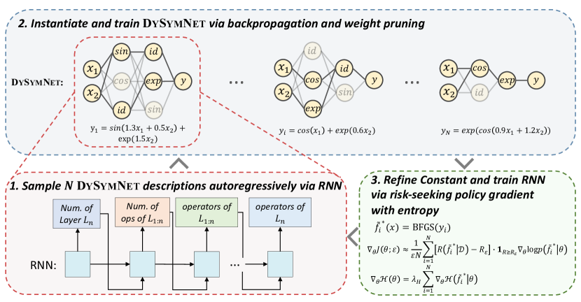
Figure 2: Overview of neural-guided DySymNet. First, we sample batch descriptions of DySymNet architecture autoregressively via RNN. Then, we instantiate and train DySymNet through backpropagation and weight pruning. Finally, we use BFGS to refine the constants and train RNN via risk-seeking policy gradient with entropy.

DySymNet architecture

In this work, DySymNet is flexible and adaptable in architecture, rather than being fixed and unchanging. The architecture of the symbolic network is controlled by a recurrent neural network (RNN), with further details explained in Section 3.2. Each symbolic network is a fully connected feed-forward network with units representing the building blocks of algebraic expressions. Each layer of the DySymNet is automatically designed by the RNN for a specific SR task, and it is subject to evolve over time. In a DySymNet with $L$ layers, there are $L-1$ hidden layers that consist of a linear mapping followed by non-linear transformations. The linear mapping at level $l$ maps the $n^{\prime}$-dimensional input $\bm{h}^{(\ell-1)}$ to the $m$-dimensional intermediate representation $\bm{z}$ given by

$$\bm{z}^{(\ell)}=\bm{W}^{(\ell)}\bm{h}^{(\ell-1)}+\bm{b}^{(\ell)},$$

where $\bm{h}^{(\ell-1)}\in\mathbb{R}^{n^{\prime}}$ is the output of the previous layer, with the convention $\bm{h}^{(0)}=\bm{x}$. The weight matrix $\bm{W}^{(\ell)}\in\mathbb{R}^{m\times n^{\prime}}$ and the bias vector $\bm{b}^{(\ell)}\in\mathbb{R}^{d}$ are free parameters that learned during training. In practice, we predefine a function library $\mathcal{F}$ of available operators, e.g., $\{\textrm{Id},+,-,\times,\sin(\cdot),\cos(\cdot),\exp(\cdot)\}$, to be selected in generating DySymNet. Suppose that we have presently instantiated a specific symbolic network, whereby its $\ell$-th layer contains $u$ unary operator units, $f_{i}:\mathbb{R}\to\mathbb{R}$, for $i=1,\dots,u$, and $v$ binary operator units, $g_{i}:\mathbb{R}\times\mathbb{R}\to\mathbb{R}$ for $j=1,\dots,v$. The $\ell$-th layer output $\bm{h}^{(\ell)}$ is formed by the concatenation of units outputs

$$\bm{h}^{(\ell)}:= \left(f_{1}\left(\bm{z}_{1}^{(\ell)}\right),f_{2}\left(\bm{z}_{2}^{(\ell)}\right),\ldots,f_{u}\left(\bm{z}_{u}^{(\ell)}\right)\right.,$$

$$\left.g_{1}\left(\bm{z}_{u+1}^{(\ell)},\bm{z}_{u+2}^{(\ell)}\right),\ldots,g_{v}\left(\bm{z}_{u+2v-1}^{(\ell)},\bm{z}_{u+2v}^{(\ell)}\right)\right).$$

Specifically, the non-linear transformation stage has $n=u+v$ outputs and $m=u+2v$ inputs. The unary units, $f_{1},\dots,f_{u}$, $f_{i}\in\{\textrm{Id},\sin(\cdot),\cos(\cdot),\exp(\cdot)\}$, receive the respective component, $z_{1},\dots,z_{u}$ as inputs. The binary units $g_{1},\dots,g_{v}$, $g_{j}\in\{+,-,\times,\div\}$, receive the remaining component, $z_{u+1},\dots,z_{u+2v}$, as input in pairs of two. For example, the multiplication unit computes the product of their two input values: $g_{j}(\bm{z}_{u+2j-1},\bm{z}{u+2j}):=\bm{z}_{u+2j-1}\cdot\bm{z}_{u+2j}$, for $j=1,\dots,v.$

The last layer computes the regression values by a linear read-out without any operator units

$$\bm{y}^{(L)}:=\bm{W}^{(L)}\bm{h}^{(L)}+\bm{b}^{(L)}.$$

The architecture of the symbolic network is illustrated in Figure 2. We define the expression denoted from the particular symbolic network as $\tilde{f}(\cdot)$.

DySymNet training

Similar to conventional fully-connected neural networks, the symbolic network possesses its own set of free parameters, denoted as $\bm{\Theta}=\{\bm{W}^{(1)},\dots,\bm{W}^{(L)},\bm{b}^{(1)},\dots,\bm{b}^{(L)}\}$, which is predetermined and can undergo end-to-end training through back-propagation. While it may be possible to fit a more accurate expression that incorporates a greater number of terms, for a successful SR method, the goal is to find the simplest expression that accurately explains the dataset. This requires a trade-off between accuracy and complexity. To achieve this, two approaches are adopted. First, similar to the transformer-based methods that impose constraints on the pre-order traversal length of the expression tree, we limit the maximum depth of the symbolic network to 5 layers and the maximum width to 6 neurons prior to training. Second, regularization techniques are applied during training to sparsify the weights, followed by pruning according to specific rules to obtain a simplified mathematical expression that accurately explains the dataset. More specifically, given the dataset $\mathcal{D}=\{(\bm{x_{i}},y_{i})\}_{i=1}^{n}$, the training objective is then given in the following:

$$\mathcal{L}=\frac{1}{n}\sum^{n}_{i=1}\|\tilde{f}(\bm{x}_{i})-y_{i}\|^{2}+\lambda\sum^{L}_{\ell=1}|\bm{\Theta}^{(\ell)}|_{r}$$

where $n$ indicates the size of training data, the last term represents the regularization term, $\lambda$ is a switch factor of the regularization term, with a value of $\{0,1\}$, and $L$ is the number of hidden layers.

Furthermore, we propose an adaptive gradient clipping strategy to enhance the stability of the training process. Specifically, the gradient norm at each time step is calculated as the moving average of the gradient norm within a certain time window. Then, this average value is used to adjust the threshold $\gamma$ for gradient clipping, which is applied to the gradients of DySymNet. The gradient clipping threshold with window size $w$ and weight factor $c$ during the $n$-th epoch of training DySymNet is given by: $\gamma=\frac{c}{w}\sum_{i=1}^{w}\sum_{\ell=1}^{L}\|\Theta^{(\ell)}\|_{2}$, where we set the window size $w$ is 50 and the weight factor $c$ is 0.1. In the ablation experiments in Section 4.5, we demonstrated the effectiveness of this technique.

Regularization and prune

The purpose of regularization is to obtain a sparse symbolic network, which is consistent with the goal of SR to obtain an interpretable and concise expression. The ideal scenario would involve directly minimizing the $L_{0}$ norm, wherein the regularization term penalizes the presence of non-zero weights irrespective of their magnitude, effectively pushing the solution towards sparse representations. However, the utilization of $L_{0}$ regularization presents a combinatorial conundrum that is NP-hard to solve, thus rendering it incompatible with gradient descent methods that are typically employed for optimizing neural networks. $L_{1}$ regularization has long been recognized as a prominent sparsity technique, which is used in the original EQL (Sahoo et al., 2018). Despite its effectiveness in promoting sparsity, since $L_{1}$ regularization also penalizes the magnitude of the weights, $L_{0.5}$ has been proposed to enforce sparsity more strongly without penalizing the magnitude of the weights as much as $L_{1}$ (Xu et al., 2010; Zong-Ben et al., 2012). Following (Kim et al., 2020), we use a smoothed version of $L_{0.5}^{*}$ proposed in (Wu et al., 2014) that has been shown to avoid singularity in the gradient, a challenge often encountered in gradient descent-based optimization when the weights approach zero. The $L_{0.5}^{*}$ regularizer employs a piecewise function to smooth out the function at small magnitudes:

$$L_{0.5}^{*}(w)=\begin{cases}|w|^{1/2}&|w|\geq a\\ \left(-\frac{w^{4}}{8a^{3}}+\frac{3w^{2}}{4a}+\frac{3a}{8}\right)^{1/2}&|w|<a\end{cases},$$

where $a\in\mathbb{R}^{+}$ is the transition point between the standard $L_{0.5}$ function and the smoothed function. After training, we keep all weights $w\in\bm{W}^{1\dots L}$ that are close to 0 at 0, i.e., if $|w|<0.01$ then $w=0$ to obtain the sparse structure.

3.2 Generate DySymNet with a controller recurrent neural network

We leverage a controller to generate architecture descriptions of DySymNet. The controller is implemented as an RNN. We can use the RNN to generate architecture parameters as a sequence of tokens sequentially. Once the RNN finishes generating an architecture, a DySymNet with this architecture is instantiated and trained. At convergence, we obtain the compact symbolic expression and evaluate it with a reward function. The reward function is not differentiable with respect to the parameters of the controller RNN, $\theta_{c}$; thus, we optimize $\theta_{c}$ via policy gradient in order to maximize the expected reward of the proposed architectures. Next, we will elaborate on the specific process of generating architecture parameters of DySymNet using the RNN, the reward function definition, and the training algorithm.

Generative process

We adopt a Markov Decision Process (MDP) (Sutton and Barto, 2018) modeling the process of generating architectures. An RL setting consists of four components ($\mathcal{S},\mathcal{A},\mathcal{P},\mathcal{R}$) in a MDP. In this view, the list of tokens that the controller RNN predicts can be viewed as a list of actions $a_{1:T}\in\mathcal{A}$ to design an architecture for a DySymNet. Hence, the process of generating architectures can be framed in RL as follows: the agent (RNN) emits a distribution over the architecture $p(a_{1:T}|\theta_{c})$, observes the environment (current architecture) and, based on the observation, takes an action (next available architecture parameter) and transitions into a new state (new architecture). The architecture parameters of the DySymNet mainly consist of three parts: the number of layers, the number of operators for each layer, and the type of each operator. As shown in Figure 2, for a specific process, the RNN first samples the number of layers in the network. Then, for each layer, the RNN samples the number of operators in the $i$-th layer and the type of operators sequentially. At each time step, the input vector $\bm{x}_{t}$ of the RNN is obtained by embedding the previous parameter $a_{t-1}$. Each episode refers to the complete process of using the RNN to sample a DySymNet, instantiating it, and training it to obtain a symbolic expression. This process is performed iteratively until the resulting expression meets the desired performance criteria.

Reward definition

As the expression $\tilde{f}(\cdot)$ identified from the DySymNet can only be evaluated at the end of the episode, the reward $R$ equals 0 until the final step is reached. Then, we use the nonlinear optimization algorithm BFGS (Fletcher, 1984) to refine the constants to get a better-fitting expression $\tilde{f}^{*}(\cdot)$. The constants in the expression $\tilde{f}(\cdot)$ are used as the initial values for the BFGS algorithm. To align with the training objective of the DySymNet, we first calculate the standard fitness measure mean squared error (MSE) between the ground-truth target variable $y$ and the predicted target variable $\tilde{y}=\tilde{f}^{*}(\bm{x})$. That is, given a dataset $\mathcal{D}=\{(\bm{x_{i}},y_{i})\}_{i=1}^{n}$ of size $n$ and candidate expression $\tilde{f}^{*}(\cdot)$, $\textrm{MSE}(\tilde{f}^{*}(\bm{x}),y)=\frac{1}{n}\sum^{n}_{i=1}(\tilde{f}^{*}(\bm{x}_{i})-y_{i})^{2}$. Then, to bound the reward function, we apply a squashing function: $R(\tilde{f}^{*}|\mathcal{D})={1}/(1+\textrm{MSE})$.

Training the RNN using policy gradients

We use the accuracy of $\tilde{f}^{*}(\cdot)$ as the reward signal and use RL to train the controller RNN. More concretely, to find the optimal architecture of DySymNet, we first consider the standard REINFORCE policy gradient (Williams, 1992) objective to maximize $J_{\textrm{std}}(\theta_{c})$, defined as the expectation of a reward function $R(\tilde{f}^{*}|\mathcal{D})$ under expressions from the policy:

$$J_{\textrm{std}}(\theta_{c})\doteq\mathbb{E}_{\tilde{f}\sim p(a_{1:T}|\theta_{c})}\left[R(\tilde{f}^{*}|\mathcal{D})\right]$$

The standard policy gradient objective, $J_{\textrm{std}}(\theta_{c})$, is the desired objective for control problems in which one seeks to optimize the average performance of a policy. However, the final performance in domains like SR is measured by the single or few best-performing samples found during training. For SR, $J_{\textrm{std}}(\theta_{c})$ is not an appropriate objective, as there is a mismatch between the objective being optimized and the final performance metric. To address this disconnect, we adopt the risk-seeking policy gradient proposed in (Petersen et al., ), with a new learning objective that focuses on learning only on maximizing best-case performance. The learning objective $J_{\textrm{risk}}(\theta_{c};\varepsilon)$ is parameterized by $\varepsilon$:

$$J_{\textrm{risk}}(\theta_{c};\varepsilon)\doteq\mathbb{E}_{\tilde{f}\sim p(a_{1:T}|\theta_{c})}\left[R(\tilde{f}^{*}|\mathcal{D})\mid R(\tilde{f}^{*}|\mathcal{D})\geq R_{\varepsilon}(\theta_{c})\right],$$

where $r_{\varepsilon}(\theta_{c})$ is defined as the $(1-\varepsilon)$-quantile of the distribution of rewards under the current policy. This objective aims to increase the reward of the top $\varepsilon$ fraction of samples from the distribution, without regard for samples below that threshold. Lastly, in accordance with the maximum entropy RL framework (Haarnoja et al., 2018), we add an entropy term $\mathcal{H}$ weighted by $\lambda_{\mathcal{H}}$, to encourage exploration:

$$J_{\textrm{entropy}}(\theta_{c};\varepsilon)\doteq\mathbb{E}_{\tilde{f}\sim p(a_{1:T}|\theta_{c})}[\mathcal{H}(\tilde{f}|\theta_{c})\mid R(\tilde{f}^{*}|\mathcal{D})\geq R_{\varepsilon}(\theta_{c})].$$

4 Experiments and Results

4.1 Metrics

We assess our method using the two popular metrics: the coefficient of determination ($R^{2}$) and MSE:

$$R^{2}=1-\frac{\sum_{i}^{N_{\text{test}}}\left(y_{i}-\tilde{y}_{i}\right)^{2}}{\sum_{i}^{N_{\text{test}}}\left(y_{i}-\bar{y}\right)^{2}},\quad\quad\quad\operatorname{MSE}=\frac{1}{N_{\text{test}}}\sum_{i=1}^{N_{\text{test}}}(y_{i}-\tilde{y}_{i})^{2}$$

where $N_{\text{test}}$ is the number of observations, $y_{i}$ is the ground-truth value for the $i$-th observation, $\tilde{y}_{i}$ is the predicted value for the $i$-th observation, and $\bar{y}$ is the averaged value of the ground-truth. $R^{2}$ measures the goodness of fit of a model to the data, and it ranges from 0 to 1, with higher values indicating a better fit between the model and the data. MSE measures the average squared difference between the predicted and ground-truth values, and it ranges from 0 to positive infinity, with smaller values indicating better performance.

4.2 Baselines

SRBench (La Cava et al., 2021) has reported the performance of 14 SR methods and 7 machine learning methods on Feynman, Black-box, and Strogatz datasets from PMLB (Olson et al., 2017). We briefly introduce these methods in Appendix C. In addition, we compare the performance of our method against three other state-of-the-art SR algorithms currently:

• A Unified Framework for Deep Symbolic Regression (uDSR). A modular, unified framework for symbolic regression that integrates five disparate SR solution strategies (Landajuela et al., 2022).

• Deep Symbolic Optimization (DSO). A symbolic regression method combining GP and RL (Mundhenk et al., 2021), the current state-of-the-art algorithm, superseding DSR (Petersen et al., ).

• Neural Symbolic Regression that Scales (NeSymReS). A transformer-based symbolic regression method based on large-scale supervised training (Biggio et al., 2021).

All details for baselines are reported in Appendix D.

4.3 Benchmark problem sets

To facilitate quantitative benchmarking of our and other SR algorithms, we conducted evaluations and comparisons on almost all publicly available benchmark datasets in the SR field. We categorized these datasets into two groups, consisting of eight benchmark datasets. One group comprises four low-dimensional datasets ($d\leq 2$) that we named Standard benchmarks. They are widely used by current SR methods, including the Nguyen benchmark (Uy et al., 2011), Nguyen* (Nguyen with constants) (Petersen et al., ), Constant, Keijzer (Keijzer, 2003), Livermore (Mundhenk et al., 2021), R rationals (Krawiec and Pawlak, 2013), Jin (Jin et al., 2019) and Koza (Koza, 1994). The complete benchmark functions are given in Appendix E. Nguyen was the main benchmark used in (Petersen et al., ). The other group is the more challenging SRBench  (La Cava et al., 2021), a living SR benchmark that includes datasets with more variables ($d\geq 2$). The SRBench includes three benchmark datasets: Feynman, Black-box, and Strogatz. The Feynman dataset comprises a total of 119 equations sourced from Feynman Lectures on Physics database series (Udrescu et al., 2020). The Strogatz dataset contains 14 SR problems sourced from the ODE-Strogatz database (La Cava et al., 2016). The Black-box dataset comprises 122 problems without ground-truth expression. The input points $(\bm{x},y)$ from these three problem sets are provided in Penn Machine Learning Benchmark (PMLB) (Olson et al., 2017) and have been examined in SRBench (La Cava et al., 2021) for the SR task.

Table 1: Average $R^{2}$ of DySymNet compared with current strong baselines on the standard benchmarks $(d\leq 2)$ and SRBench ($d\geq 2$) (La Cava et al., 2021) across 20 independent training runs, where $d$ represents the dimensionality of the problem. 95% confidence intervals are obtained from the standard error between mean $R^{2}$ on each problem set.

Data Group	Benchmark	DySymNet	uDSR	DSO	NeSymReS	EQL
		$R^{2}\uparrow$	$R^{2}\uparrow$	$R^{2}\uparrow$	$R^{2}\uparrow$	$R^{2}\uparrow$
Standard $(d\leq 2)$	Nguyen	$\textbf{0.9999}_{\pm 0.0001}$	$0.9989_{\pm 0.0000}$	$0.9848_{\pm 0.0000}$	$0.9221_{\pm 0.0000}$	$0.9758_{\pm 0.0032}$
	Nguyen*	$\textbf{0.9999}_{\pm 0.0000}$	$\textbf{0.9999}_{\pm 0.0000}$	$\textbf{0.9999}_{\pm 0.0001}$	$0.3523_{\pm 0.0000}$	$0.7796_{\pm 0.0019}$
	Constant	$\textbf{0.9992}_{\pm 0.0000}$	$0.9989_{\pm 0.0002}$	$0.9989_{\pm 0.0002}$	$0.7670_{\pm 0.0000}$	$0.9817_{\pm 0.0088}$
	Keijzer	$\textbf{0.9986}_{\pm 0.0002}$	$0.9968_{\pm 0.0000}$	$0.9912_{\pm 0.0005}$	$0.9358_{\pm 0.0000}$	$0.9446_{\pm 0.0014}$
	Livermore	$\textbf{0.9896}_{\pm 0.0001}$	$0.9670_{\pm 0.0003}$	$0.9665_{\pm 0.0005}$	$0.9195_{\pm 0.0000}$	$0.7496_{\pm 0.0002}$
	R	$0.9895_{\pm 0.0012}$	$\textbf{0.9999}_{\pm 0.0000}$	$\textbf{0.9999}_{\pm 0.0000}$	$0.9368_{\pm 0.0000}$	$0.8588_{\pm 0.0061}$
	Jin	$\textbf{1.0000}_{\pm 0.0000}$	$0.9864_{\pm 0.0002}$	$0.9942_{\pm 0.0001}$	$0.9987_{\pm 0.0000}$	$0.9921_{\pm 0.0002}$
	Koza	$\textbf{1.0000}_{\pm 0.0000}$	$0.9965_{\pm 0.0000}$	$0.9999_{\pm 0.0000}$	$0.9999_{\pm 0.0000}$	$0.7571_{\pm 0.0022}$
Data Group	Benchmark	$R^{2}\uparrow$	$R^{2}\uparrow$	$R^{2}\uparrow$	$R^{2}\uparrow$	$R^{2}\uparrow$
SRBench $(d\geq 2)$	Feynman	$\textbf{0.9931}_{\pm 0.0015}$	$0.9806_{\pm 0.0003}$	$0.9190_{\pm 0.0004}$	$0.9234_{\pm 0.0000}$	$0.5641_{\pm 0.0028}$
	Strogatz	$\textbf{0.9968}_{\pm 0.0031}$	$0.9455_{\pm 0.0003}$	$0.9534_{\pm 0.0003}$	$0.8816_{\pm 0.0000}$	$0.6511_{\pm 0.0012}$
	Black-box	$\textbf{0.8908}_{\pm 0.0028}$	$0.6697_{\pm 0.0010}$	$0.6086_{\pm 0.0021}$	$0.4226_{\pm 0.0000}$	$0.4528_{\pm 0.0107}$

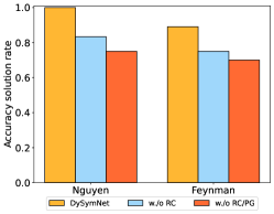
(a) without RC and RC$+$PG

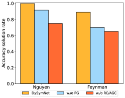
(b) without PG and RC$+$AGC

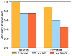
(c) without AGC and PG$+$AGC

Figure 3: Ablation study of DySymNet on Nguyen and Feynman benchmarks. The three subfigures show the performance comparison of Dysymnet without different components, including Refine Constant (RC), Policy Gradient (PG), and Adaptive Gradient Clipping (AGC).

4.4 Experimental settings

To facilitate quantitative benchmarking of our and other SR baselines described in 4.2, our approach uses the same symbol library as uDSR and DSO during testing. For uDSR and DSO, we use the hyperparameters reported in the literature (Petersen et al., ; Landajuela et al., 2022). NeSymRes is a pre-trained model on a synthetic dataset, thus its symbol library is immutable. We use the author’s released 100M model, which was trained on 100 million synthetic data. At inference, we use the settings reported in the literature (Biggio et al., 2021), with a beam size of 32 and 4 restarts of BFGS per expression. Due to the limitation of training data, NeSymReS only supports to inference the problem with up to three variables. Following (Landajuela et al., 2022), we utilize the sklearn library (Pedregosa et al., 2011) to select the top-$k$ $(k=3)$ most relevant features when inferring expressions with more than three variables on SRBench. We manually removed outliers when calculating the average $R^{2}$. Moreover, the sampling input data of standard benchmarks is the same for all methods. SRBench has already provided the data, thus obviating the need for resampling. Additional experiment details are provided in Appendix B.

4.5 Evaluation and results

Fitting accuracy on benchmarks

Table 4 reports the performance comparison results of our method with the state-of-the-art SR baselines across two group benchmarks. Notably, the problem sets in the standard benchmarks have at most two variables ($d\leq 2$) and ground-truth expressions that are relatively simple in form. Our method can quickly find the best expression without requiring many rounds of controller iteration. Thus, our method has a clear advantage in inference efficiency compared to GP-based methods, uDSR, and DSO, which require iterating through thousands of expressions to find the best one. The results indicate that DySymNet outperforms the current strong SR baselines in terms of the $R^{2}$ while maintaining a lower mean squared error (MSE). Additionally, DySymNet successfully recovered all expressions in the Jin dataset $(d=2)$ and Koza dataset. This highlights the importance of reducing the search space to find optimal expressions.

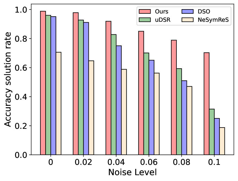
Figure 4: Acuracy solution rate of four approaches on the Standard benchmarks against increasing the noise level.

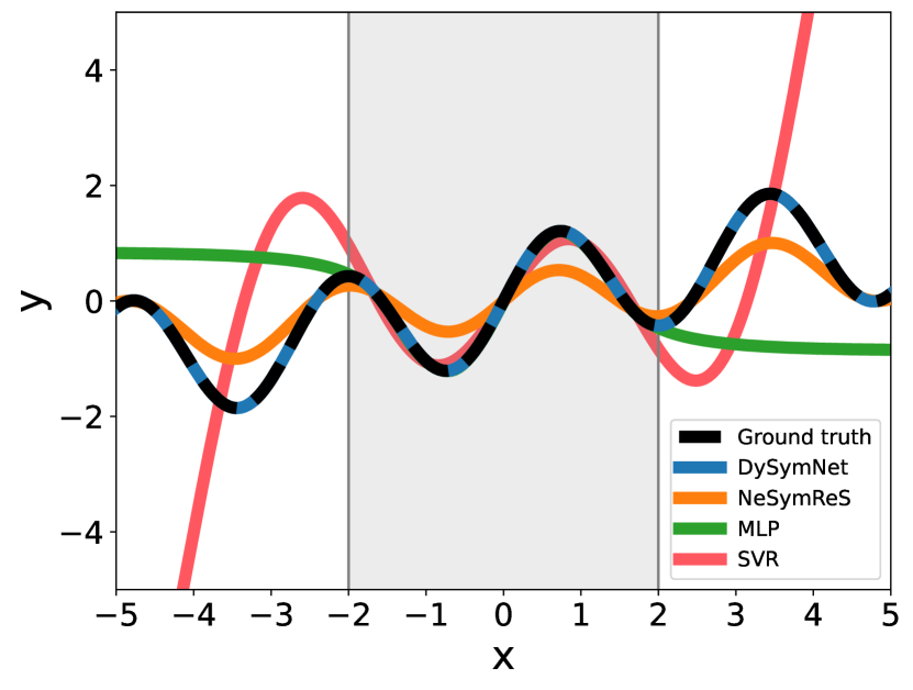
Figure 5: Extrapolation performance comparison with symbolic regression models and black-box models.

Figure 6: Training curves of RNN for the mean reward of full batch expressions identified from DySymNet.

Ablation studies

We performed a series of ablation studies to quantify the effect of each of the components. In figure 3, we show the accuracy solution rate for DySymNet on the Nguyen and Feynman benchmarks for each ablation. The results demonstrate the effectiveness of these components in improving performance.

Performance under noisy data

Since real data are almost always afflicted with measurement errors or other forms of noise, We investigated the robustness of DySymNet to noisy data by adding independent Gaussian noise to the dependent variable with mean zero and standard deviation proportional to the root-mean-square of the dependent variable in the training data. In Figure 6, we varied the proportionality constant from $0$ (noiseless) to $10^{-1}$ and evaluated each algorithm across Standard benchmarks. Accuracy solution rate is defined as the proportion for achieving $R^{2}>0.99$ on the benchmark. The experiments show that our method has the best robustness to noise, and there is no overfitting to noise when a small amount of noise is added, which is significantly better than the NeSymReS based on large-scale supervised training.

Extrapolation

Figure 6 provides a qualitative comparison between the performance of DySymNet, NeSymReS (pre-training SR method), MLP (black-box model), and SVR with regards to the ground-truth expression $2sin(1.3x)cos(x)$. The training dataset, represented by the shaded region, comprises 256 data points in the range of [-2, 2], and the evaluation is conducted on the out-of-domain region between [-5, 5]. Although all three models fit the training data very well, our proposed DySymNet outperforms the NeSymReS baseline in fitting the underlying true function, as shown by the out-of-domain performance. Additionally, the result demonstrates a strong advantage of the symbolic approach: once it has found the correct expression, it can predict the whole sequence, whereas the precision of the black-box model deteriorates as it extrapolates further.

Convergence analysis

In Figure 6, the average reward computed by the batch expressions, which are identified from DySymNet, gradually increases with each training step of the policy network RNN, indicating that the direction of the policy gradient is towards maximizing the expected reward value, and the RNN gradually converges to an optimal value.

5 Conclusion

We present a novel neural-guided dynamic symbolic network for symbolic regression. Our method provides a new search paradigm for symbolic regression and overcomes the challenges of current symbolic regression methods in solving high-dimensional problems and coefficient optimization. Through extensive numerical experiments on both low-dimensional public standard benchmarks and SRBench with more variables, we demonstrate that DySymNet achieves state-of-the-art performance in terms of fitting accuracy and robustness to noise.

Limitations

Our method may encounter difficulties when using division and logarithmic operators, although can achieve good performance without these symbols. Future work may explore additional optimization techniques, as well as the incorporation of domain-specific knowledge to enhance the performance and applicability of DySymNet in diverse fields.

Appendix for “A Neural-Guided Dynamic Symbolic Network for Exploring Mathematical Expressions from Data”

Contents:

• Appendix A: Pseudocode for DySymNet

• Appendix B: Additional experiment details

• Appendix C: Short descriptions of SRBench baselines

• Appendix D: Baselines details

• Appendix E: Standard benchmark expressions

• Appendix F: Additional experiment results

Appendix A Pseudocode for DySymNet

In this section, we provide the pseudocode for DySymNet. The overall algorithm is detailed in Algorithm 1. Moreover, we provide pseudocode for the function SampleSymbolicNetwork (line 4 of Algorithm 1) and TrainSymbolicNetwork (line 5 of Algorithm 1) in Algorithm 2 and Algorithm 3, respectively. Specifically, Algorithm 1 describes the overall framework of DySymNet. We use RNN as the controller to sample a batch of symbolic network structures and instantiate them. By training the symbolic network, we can obtain compact expressions. Then, we refine the constants using BFGS and calculate corresponding rewards. When we obtain a batch of rewards, we calculate the $\epsilon$-quantile of the rewards. We use the top $(1-\epsilon)$ rewards to calculate policy gradients and corresponding entropies to update the RNN. This iterative process continues until we reach the threshold we set.

Input: learning rate $\alpha_{c}$ of controller; entropy coefficient $\lambda_{\mathcal{H}}$; risk factor $\epsilon$; batch size $N$; sample epochs $M$; reward function $R$; early stop threshold $R_{t}$; SR problem $\mathcal{P}$ consisting of tabular data $\mathcal{D}(X,y)$

Output: Best fitting expression $\tilde{f}^{*}$

1 Initialize controller RNN with parameters $\theta_{c}$, defining distribution over symbolic network $p(\mathcal{S}_{net}|\theta_{c})$ for $i\leftarrow 1$ to $M$ do

2       for $j\leftarrow 1$ to $N$ do

3             $\mathcal{S}_{net}\leftarrow\textrm{SampleSymbolicNetwork}(\theta_{c})$ $\triangleright$ Sample a symbolic network via controller

4             $\tilde{f}_{j}\leftarrow\textrm{TrainSymbolicNetwork}(\mathcal{S}_{net},\mathcal{D})$ $\triangleright$ Train the symbolic network

5             $\tilde{f}_{j}^{*},\textrm{mse}_{j}\leftarrow\textrm{BFGS}(\tilde{f}_{j},\mathcal{D})$ $\triangleright$ Refine constants using BFGS

6             $R(\tilde{f}_{j}^{*})\leftarrow 1/(1+\textrm{mse}_{j})$ $\triangleright$ Compute reward through MSE

7             if $R(\tilde{f}_{j}^{*})>R_{t}$ then

8                  

9                  return $\tilde{f}_{j}^{*}$ $\triangleright$ Return the best expression if reach the threshold

10             end if

11            

12       end for

13      

14      $\mathcal{R}\leftarrow\{R(\tilde{f}_{j}^{*})\}_{j=1}^{N}$ $\triangleright$ Compute batch rewards

15       $R_{\epsilon}\leftarrow(1-\epsilon)$-quantile of $\mathcal{R}$ $\triangleright$ Compute reward threshold

16       $\mathcal{F}\leftarrow\{\tilde{f}_{j}^{*}:R(\tilde{f}_{j}^{*})\geq R_{\epsilon}\}$ $\triangleright$ Select subset of expressions above threshold

17       $\mathcal{R}\leftarrow\{R(\tilde{f}_{j}^{*}):R(\tilde{f}_{j}^{*})\geq R_{\epsilon}\}$ $\triangleright$ Select corresponding subset of rewards

18       $\hat{g_{1}}\leftarrow\textrm{ReduceMean}((\mathcal{R}-R_{\varepsilon})\nabla_{\theta_{c}}\log p(\mathcal{F}|\theta_{c}))$ $\triangleright$ Compute risk-seeking policy gradient

19       $\hat{g_{2}}\leftarrow\textrm{ReduceMean}(\lambda_{\mathcal{H}}\nabla_{\theta_{c}}\mathcal{H}(\mathcal{F}|\theta_{c}))$ $\triangleright$ Compute risk-seeking policy gradient

20       $\theta_{c}\leftarrow\theta_{c}+\alpha(\hat{g_{1}}+\hat{g_{2}})$ $\triangleright$ Apply gradients

21 end for

Algorithm 1 A neural-guided dynamic symbolic network for symbolic regression

Algorithm 2 describes the specific process of using RNN to sample a symbolic network structure, which is corresponding to Generative process of Section 3.2. In a particular sampling process, we first sample from the number library of layers to determine the current number of layers in the symbolic network. Then, we iterate through each layer to decide the number of operators and operator categories for each layer. Once a complete symbolic network structure has been sampled, we instantiate it. The various libraries of symbolic network structure are reported in Table 2.

Input: RNN with parameters $\theta_{c}$; number library for symbolic network layers $\mathcal{L}_{L}$; number library for operators in each layer $\mathcal{L}_{n}$; operators library $\mathcal{L}_{o}$

Output: Symbolic network $\mathcal{S}_{net}$

1

2$c_{0}\leftarrow\vec{0}$ $\triangleright$ Initialize RNN cell state to zero

3 $x\leftarrow\textrm{rand}()$ $\triangleright$ Initialize input randomly

4 $(\psi_{L}^{(1)},c_{1})\leftarrow$ RNN_Cell$(x,c_{0};\theta_{c})$ $\triangleright$ Emit probabilities over $\mathcal{L}_{L}$; update state

5 $L\leftarrow\textrm{Categorical}(\psi_{L}^{(1)})$ $\triangleright$ Sample a value from $\mathcal{L}_{L}$ as the number of layers

6 $x\leftarrow\psi_{L}^{(1)}$ $\triangleright$ Take the probabilities over $\mathcal{L}_{L}$ as input

7 for $i\leftarrow 1$ to $L$ do

8       $(\psi_{n}^{(i)},c_{i})\leftarrow$ RNN_Cell$(x,c_{i-1};\theta_{c})$ $\triangleright$ Emit probabilities over $\mathcal{L}_{n}$; update state

9       $n^{(i)}=\textrm{Categorical}(\psi_{n}^{(i)})$ $\triangleright$ Sample a value from $\mathcal{L}_{n}$ as the number of operators for layer $L^{i}$

10       $x\leftarrow\psi_{n}^{(i)}$ $\triangleright$ Take the probabilities over $\mathcal{L}_{n}$ as input

11       $(\psi_{o}^{(i)},c_{i})\leftarrow$ RNN_Cell$(x,c_{i-1};\theta_{c})$ $\triangleright$ Emit probabilities over $\mathcal{L}_{o}$; update state

12       $o^{(i)}\leftarrow\textrm{Categorical}(\psi_{o}^{(i)})$ $\triangleright$ Sample $n^{i}$ operators for layer $L^{i}$

13       $x\leftarrow\psi_{o}^{(i)}$ $\triangleright$ Take the probabilities over $\mathcal{L}_{o}$ as input

14      

15 end for

16$\mathcal{S}_{net}\leftarrow\textrm{Instantiation}(L,n,o)$ $\triangleright$ Instantiate a corresponding symbolic network

17 return $\mathcal{S}_{net}$

Algorithm 2 Sample a symbolic network autoregressively via controller RNN

Algorithm 3 describes the specific process of training a symbolic network, which is corresponding to Section 3.1. We divide the training process into two stages. In the first stage, we use MSE loss to supervise and converge the weights of the symbolic network to an appropriate interval. In the second stage, we add $L_{0.5}^{*}$ regularization term to sparse the symbolic network and finally perform pruning to obtain a compact expression. We use the adaptive gradient clipping technology described in Section 3.1 in both stages, which makes the training process of the symbolic network more stable.

Input: learning rate $\alpha_{s}$, regulation weight $\lambda$; training epochs $n_{1}$; training epochs $n_{2}$; window size $w$; weight clipping factor $c$; clipping threshold $\gamma$; pruning threshold $\beta$

Output: expression $\tilde{f}$

1 Initialize symbolic network with parameters $\bm{\Theta}$

2 $\textrm{queue}\leftarrow[]$ $\triangleright$ Initialize gradient norm queue

3 for $i\leftarrow 1$ to $n_{1}$ do

4       $J(\bm{\Theta})\leftarrow\textrm{MSE}(y,\tilde{y})$ $\triangleright$ Compute MSE loss

5       $\textrm{queue}.\textrm{append}(\|\bm{\Theta}\|_{2})$ $\triangleright$ Append current gradient norm to queue

6       if len(queue) > $w$ then

7             queue.popleft()

8       end if

9      $\gamma\leftarrow\frac{c}{w}\sum_{i=1}^{w}\sum_{\ell=1}^{L}\|\bm{\Theta}^{(\ell)}\|_{2}$ $\triangleright$ Compute gradient clipping threshold

10       $g\leftarrow\textrm{clip\_grad\_norm}(\bm{\Theta},\gamma)$ $\triangleright$ Clip gradient

11       $\bm{\Theta}\leftarrow\bm{\Theta}-\alpha_{s}\nabla J(\bm{\Theta})$ $\triangleright$ Apply gradient

12 end for

13for $i\leftarrow 1$ to $n_{2}$ do

14       $J(\bm{\Theta})\leftarrow\textrm{MSE}(y,\tilde{y})+\lambda L_{0.5}^{*}(\bm{\Theta})$ $\triangleright$ Compute MSE loss and regularizaiton loss

15       $\textrm{queue}.\textrm{append}(\|\bm{\Theta}\|_{2})$ $\triangleright$ Append current gradient norm to queue

16       if len(queue) > $w$ then

17             queue.popleft()

18       end if

19      $\gamma\leftarrow\frac{c}{w}\sum_{i=1}^{w}\sum_{\ell=1}^{L}\|\bm{\Theta}^{(\ell)}\|_{2}$ $\triangleright$ Compute gradient clipping threshold

20       $g\leftarrow\textrm{clip\_grad\_norm}(\bm{\Theta},\gamma)$ $\triangleright$ Clip gradient

21       $\bm{\Theta}\leftarrow\bm{\Theta}-\alpha_{s}\nabla J(\Theta)$ $\triangleright$ Apply gradient

22 end for

23$\tilde{f}\leftarrow\textrm{Pruning}(\bm{\Theta},\beta)$ $\triangleright$ Pruning and using Sympy to convert to corresponding expression

24 return $\tilde{f}$

Algorithm 3 Training process of symbolic network

Appendix B Additional experiment details

In this section, we describe additional experimental details, including the experimental environment, hyperparameter settings of our approach and other baselines.

Computing infrastructure

Experiments in this work were executed on an Intel Xeon Platinum 8255C CPU @ 2.50GHz, 32GB RAM equipped with NVIDIA Tesla V100 GPUs 32 GB.

Hyperparameter settings

The hyperparameters of our method mainly include three parts, which are the hyperparameters of controller RNN, the hyperparameters of symbolic network training, and the hyperparameters of symbolic network structure. For the RNN, the space of hyperparameters considered was learning rate $\in\{0.0003,0.0006,0.001\}$, and entropy weight $\lambda_{\mathcal{H}}\in\{0.001,0.005,0.01\}$. For the symbolic network training, the space of hyperparameters considered was learning rate $\in\{0.01,0.05,0.1\}$, weight pruning threshold $\beta\in\{0.001,0.01,0.05\}$, adaptive gradient clipping $\in\{\textsc{True},\textsc{False}\}$, window size $w\in\{10,50,100\}$, and add bias $\in\{\textsc{True},\textsc{False}\}$. Adding bias can further improve the performance of the algorithm, but it also increases the complexity of the final expression. We tuned hyperparameters by performing grid search on benchmarks Nguyen-5 and Nguyen-10. We selected the hyperparameters combination with the highest average $R^{2}$. The best found hyperparameters are listed in Table 2 and used for all experiments and all benchmark expressions. For the symbolic network structure, there are three categories of hyperparameters that are the number of layers, the number of operators for each layer, and the type of each operator. Notably, these parameters differ from the model training parameters. Each structural parameter is a set that RNN can choose from during sampling, and there is no optimal value for them, as they only determine the upper limit of the symbolic network’s representational capacity, similar to the maximum sequence length defined in DSO (Mundhenk et al., 2021). Thus, the selection of these parameters can be adjusted based on specific scenarios to achieve the best results. For fair comparison, we used the same structural hyperparameter in all experiments, where the operator library was consistent with that of uDSR and DSO.

Table 2: Hyperparameters for DySymNet.

Hyperparameter	Symbol	Value
RNN Parameters
Learning rate	$\alpha_{c}$	0.0006
Entropy weight	$\lambda_{\mathcal{H}}$	0.005
RNN cell size	–	32
RNN cell layers	–	1
Risk factor	$\epsilon$	0.5
Symbolic network training parameters
Learning rate	$\alpha_{s}$	0.1
Regularization weight	$\lambda$	0.005
Weight pruning threshold	$\beta$	0.01
Training epochs (stage 1)	$n_{1}$	10000
Training epochs (stage 2)	$n_{2}$	10000
Adaptive gradient clipping	–	True
Window size	$w$	50
Add bias	–	False
Symbolic network structure parameters
Operators library	–	$\{+,-,\times,\sin,\cos,\tan,\exp,\mathord{\color[rgb]{0.67,0.67,0.67}\bullet}^{2}\}$
Number library of layers	–	$\{1,2,3,4,5\}$
Number library of operators for each layer	–	$\{1,2,3,4,5,6\}$

Appendix C Short descriptions of the 14 original SRBench baselines

Herein, we present concise descriptions of the 14 SR baseline methodologies employed by SRBench, as depicted in Figure 1. These 14 methods include both GP-based and deep learning-based approaches and do not encompass seven other well-known machine learning methods.

• Bayesian symbolic regression (BSR): Jin et al. (2019) present a method that incorporates prior knowledge and generates expression trees from a posterior distribution by utilizing a highly efficient Markov Chain Monte Carlo algorithm. This approach is impervious to hyperparameter settings and yields more succinct solutions as compared to solely GP-based methods.

• AIFeynman: AIFeynman (Udrescu et al., 2020) exploits knowledge of physics and the given training data, by identifying simplifying properties (e.g., multiplicative separability) of the underlying functional form. They decompose a larger problem into several smaller sub-problems and resolve each sub-problem through brute-force search.

• Age-fitness Pareto optimization (AFP): Schmidt and Lipson (2010) propose a genetic programming (GP) approach that mitigates premature convergence by incorporating a multidimensional optimization objective that assesses solutions based on both their fitness and age.

• AFP with co-evolved fitness estimates (AFP-FE): Schmidt and Lipson (2009) expands on  (Schmidt and Lipson, 2008) by adding a new fitness estimation approach.

• $\epsilon$-lexicase selection (EPLEX): La Cava et al. (2019) present an approach that enhances the parent selection procedure in GP by rewarding expressions that perform well on more challenging aspects of the problem rather than assessing performance on data samples in aggregate or average.

• Feature engineering automation tool (FEAT): La Cava et al. (2018) present a strategy for discovering simple solutions that generalize well by storing solutions with accuracy-complexity trade-offs to increase generalization and interpretation.

• Fast function extraction (FFX): McConaghy (2011) propose a non-evolutionary SR technique based on pathwise learning (Friedman et al., 2010) that produces a set of solutions that trade-off error versus complexity while being orders of magnitude faster than GP and giving deterministic convergence.

• GP (gplearn): The open source library gplearn (https://github.com/trevorstephens/gplearn) is used in Koza-style GP algorithms. This implementation is very similar to the GP component in DSO and uDSR.

• GP version of the gene-pool optimal mixing evolutionary algorithm (GP-GOMEA): Virgolin et al. (2021) propose combining GP with linkage learning, a method that develops a model of interdependencies to predict which patterns will propagate and proposes simple and interpretable solutions.

• Deep symbolic regression (DSR): Petersen et al. leverage a recurrent neural network to sample the pre-order traversal of the expression guiede by the proposed risk-seeking gradient.

• Interaction-transformation evolutionary algorithm (ITEA): de Franca and Aldeia (2021) present a mutation-based evolutionary algorithm based on six mutation heuristics that allows for the learning of high-performing solutions as well as the extraction of the significance of each original feature of a data set as an analytical function.

• Multiple regression genetic programming (MRGP): As a cost-neutral modification to basic GP, Arnaldo et al. (2014) describe an approach that decouples and linearly combines sub-expressions via multiple regression on the target variable.

• SR with Non-Linear least squares (Operon): Kommenda et al. (2020) improve generalization by including nonlinear least squares optimization into GP as a local search mechanism for offspring selection.

• Semantic backpropagation genetic programming (SBP-GP): Virgolin et al. (2019) improve the random desired operator algorithm (Pawlak et al., 2014), a semantic backpropagation-based GP approach, by introducing linear scaling concepts, making the process significantly more effective despite being computationally more expensive.

Appendix D Baselines details

A Unified Framework for Deep Symbolic Regression (uDSR)

Landajuela et al. (2022) proposed a modular, unified framework for SR that integrates five disparate SR solution strategies. In this work, we use the open-source code and implementation provided by the authors. To ensure fair comparison, we use the same symbol library as our algorithm and add the const token to give it the ability to generate constants. In addition, we used the hyperparameter combination for training reported in the literature.

Deep Symbolic Optimization (DSO)

DSO (Mundhenk et al., 2021) is a hybrid method that combines RL and GP. They use a policy network to seed the starting population of a GP algorithm. In this work, we use the open-source code and implementation provided by the authors. To ensure fair comparison, we use the same symbol library as our algorithm and add the const token to give it the ability to generate constants. In addition, we used the hyperparameter combination for training reported in the literature.

Neural Symbolic Regression that Scales (NeSymReS)

NeSymReS (Biggio et al., 2021) is a transformer-based model for SR. It is trained on synthetic data with a scale of 10M and 100M. In this work, we use the open-source code and implementation provided by the authors, following their proposal, and using their released 100M model. To ensure fair comparison, we use the settings reported in the literature, with a beam size of 32 and 4 restarts of BFGS per expression. As NeSymReS was only trained on a dataset with variables $d\leq 3$, we utilize the sklearn library (Pedregosa et al., 2011) to select the top three most relevant features when inferring benchmark expressions with more than three variables.

Appendix E Standard benchmark expressions

This section describes the exact expressions in the standard benchmarks ($d\leq 2$) used to compare our method with the current state-of-the-art baselines. In table LABEL:tab:benchmarks, we show the name of the benchmark, corresponding expressions, and dataset information. For fair comparison, the dataset used in all methods was generated under the same seed.

Table 3: Standard benchmark symbolic regression problem specifications. Input variables are denoted by $x$ and/or $y$. $U\left(a,b,c\right)$ denotes $c$ random points uniformly sampled between $a$ and $b$ for each input variable; training and test datasets use different random seeds.

Name	Expression	Dataset
Nguyen-1	$x^{3}+x^{2}+x$	$U\left(-1,1,256\right)$
Nguyen-2	$x^{4}+x^{3}+x^{2}+x$	$U\left(-1,1,256\right)$
Nguyen-3	$x^{5}+x^{4}+x^{3}+x^{2}+x$	$U\left(-1,1,256\right)$
Nguyen-4	$x^{6}+x^{5}+x^{4}+x^{3}+x^{2}+x$	$U\left(-1,1,256\right)$
Nguyen-5	$\sin(x^{2})\cos(x)-1$	$U\left(-3,3,256\right)$
Nguyen-6	$\sin(x)+\sin(x+x^{2})$	$U\left(-3,3,256\right)$
Nguyen-7	$\log(x+1)+\log(x^{2}+1)$	$U\left(0,2,256\right)$
Nguyen-8	$\sqrt{x}$	$U\left(0,4,256\right)$
Nguyen-9	$\sin(x)+\sin(y^{2})$	$U\left(0,1,256\right)$
Nguyen-10	$2\sin(x)\cos(y)$	$U\left(0,1,256\right)$
Nguyen-11	$x^{y}$	$U\left(0,1,256\right)$
Nguyen-12	$x^{4}-x^{3}+\frac{1}{2}y^{2}-y$	$U\left(0,1,256\right)$
Nguyen-1c	$3.39x^{3}+2.12x^{2}+1.78x$	$U\left(-1,1,256\right)$
Nguyen-5c	$\sin(x^{2})\cos(x)-0.75$	$U\left(-1,1,256\right)$
Nguyen-7c	$\log(x+1.4)+\log(x^{2}+1.3)$	$U\left(0,2,256\right)$
Nguyen-8c	$\sqrt{1.23x}$	$U\left(0,4,256\right)$
Nguyen-10c	$\sin(1.5x)\cos(0.5y)$	$U\left(0,1,256\right)$
Constant-1	$3.39x^{3}+2.12x^{2}+1.78x$	$U\left(-1,1,256\right)$
Constant-2	$\sin{(x^{2})}\cos{(x)}-0.75$	$U\left(-1,1,256\right)$
Constant-3	$\sin{(1.5x)}\cos{(0.5y)}$	$U\left(0,1,256\right)$
Constant-4	$2.7x^{y}$	$U\left(0,1,256\right)$
Constant-5	$\sqrt{1.23x}$	$U\left(0,4,256\right)$
Constant-6	$x^{0.426}$	$U\left(0,2,256\right)$
Constant-7	$2\sin{(1.3x)}\cos{(y)}$	$U\left(-1,1,256\right)$
Constant-8	$\log(x+1.4)+\log(x^{2}+1.3)$	$U\left(0,2,256\right)$
Keijzer-3	$0.3\cdot x\cdot\sin{(2\cdot\pi\cdot x)}$	$U\left(-1,1,256\right)$
Keijzer-4	$x^{3}\exp{(-x)}\cos{(x)}\sin{(x)}({\sin{x}}^{2}\cos{x}-1)$	$U\left(-1,1,256\right)$
Keijzer-6	$\frac{x\cdot(x+1)}{2}$	$U\left(-1,1,256\right)$
Keijzer-7	$\ln{x}$	$U\left(1,2,256\right)$
Keijzer-8	$\sqrt{x}$	$U\left(0,1,256\right)$
Keijzer-9	$\log{(x+\sqrt{(x^{2}+1)})}$	$U\left(-1,1,256\right)$
Keijzer-10	$x^{y}$	$U\left(0,1,256\right)$
Keijzer-11	$xy+\sin{((x-1)(y-1))}$	$U\left(-1,1,256\right)$
Keijzer-12	$x^{4}-x^{3}+\frac{y^{2}}{2}-y$	$U\left(-1,1,256\right)$
Keijzer-13	$6\sin{(x)}\cos{(y)}$	$U\left(-1,1,256\right)$
Keijzer-14	$\frac{8}{2+x^{2}+y^{2}}$	$U\left(-1,1,256\right)$
Keijzer-15	$\frac{x^{3}}{5}+\frac{y^{3}}{2}-y-x$	$U\left(-1,1,256\right)$
Livermore-1	$\frac{1}{3}+x+\sin\left({x}^{2}\right)$	$U\left(-5,5,256\right)$
Livermore-2	$\sin\left({x}^{2}\right)\cos\left(x\right)-2$	$U\left(-1,1,256\right)$
Livermore-3	$\sin\left({x}^{3}\right)\cos\left({x}^{2}\right)-1$	$U\left(-1,1,256\right)$
Livermore-4	$\log(x+1)+\log({x}^{2}+1)+\log(x)$	$U\left(0,2,256\right)$
Livermore-5	${x}^{4}-{x}^{3}+{x}^{2}-y$	$U\left(-1,1,256\right)$
Livermore-6	$4{x}^{4}+3{x}^{3}+2{x}^{2}+x$	$U\left(-1,1,256\right)$
Livermore-7	$\sinh(x)$	$U\left(-1,1,256\right)$
Livermore-8	$\cosh(x)$	$U\left(-1,1,256\right)$
Livermore-9	${x}^{9}+{x}^{8}+{x}^{7}+{x}^{6}+{x}^{5}+{x}^{4}+{x}^{3}+{x}^{2}+x$	$U\left(-1,1,256\right)$
Livermore-10	$6\sin\left(x\right)\cos\left(y\right)$	$U\left(-1,1,256\right)$
Livermore-11	$\frac{{x}^{2}{x}^{2}}{x+y}$	$U\left(-1,1,256\right)$
Livermore-12	$\frac{{x}^{5}}{{y}^{3}}$	$U\left(-1,1,256\right)$
Livermore-13	${x}^{\frac{1}{3}}$	$U\left(0,1,256\right)$
Livermore-14	${x}^{3}+{x}^{2}+x+\sin\left(x\right)+\sin\left({x}^{2}\right)$	$U\left(-1,1,256\right)$
Livermore-15	${x}^{\frac{1}{5}}$	$U\left(0,1,256\right)$
Livermore-16	${x}^{\frac{2}{5}}$	$U\left(0,1,256\right)$
Livermore-17	$4\sin\left(x\right)\cos\left(y\right)$	$U\left(-1,1,256\right)$
Livermore-18	$\sin\left({x}^{2}\right)\cos\left(x\right)-5$	$U\left(-1,1,256\right)$
Livermore-19	${x}^{5}+{x}^{4}+{x}^{2}+x$	$U\left(-1,1,256\right)$
Livermore-20	$\operatorname{exp}\left({-x}^{2}\right)$	$U\left(-1,1,256\right)$
Livermore-21	${x}^{8}+{x}^{7}+{x}^{6}+{x}^{5}+{x}^{4}+{x}^{3}+{x}^{2}+x$	$U\left(-1,1,256\right)$
Livermore-22	$\operatorname{exp}\left(-0.5{x}^{2}\right)$	$U\left(-1,1,256\right)$
R-1	$\frac{{\left(x+1\right)}^{3}}{{x}^{2}-x+1}$	$U\left(-1,1,256\right)$
R-2	$\frac{{x}^{5}-3{x}^{3}+1}{{x}^{2}+1}$	$U\left(-1,1,256\right)$
R-3	$\frac{{x}^{6}+{x}^{5}}{{x}^{4}+{x}^{3}+{x}^{2}+x+1}$	$U\left(-1,1,256\right)$
Jin-1	$2.5x^{4}-1.3x^{3}+0.5y^{2}-1.7y$	$U\left(-1,1,256\right)$
Jin-2	$8.0x^{2}+8.0y^{3}-15.0$	$U\left(-1,1,256\right)$
Jin-3	$0.2x^{3}+0.5y^{3}-1.2y-0.5x$	$U\left(-1.5,1.5,256\right)$
Jin-4	$1.5\exp(x)+5.0\cos(y)$	$U\left(-1.5,1.5,256\right)$
Jin-5	$6.0\sin(x)\cos(y)$	$U\left(-1,1,256\right)$
Jin-6	$1.35xy+5.5\sin((x-1.0)(y-1.0))$	$U\left(-1,1,256\right)$
Koza-2	$x^{5}-2x^{3}+x$	$U\left(-1,1,256\right)$
Koza-3	$x^{6}-2x^{4}+x^{2}$	$U\left(-1,1,256\right)$

Appendix F Additional experiment results

Table 4: Recovery rate $A_{Rec\%}$ of DySymNet compared with current strong baselines on the standard benchmarks $(d\leq 2)$ and SRBench ($d\geq 2$) (La Cava et al., 2021) across 20 independent training runs, where $d$ represents the dimensionality of the problem. 95% confidence intervals are obtained from the standard error between mean recovery on each problem set.

Data Group	Benchmark	DySymNet	uDSR	DSO	NeSymReS	EQL
		$A_{Rec\%}\uparrow$	$A_{Rec\%}\uparrow$	$A_{Rec\%}\uparrow$	$A_{Rec\%}\uparrow$	$A_{Rec\%}\uparrow$
Standard $(d\leq 2)$	Nguyen	$\textbf{91.66}_{\pm 0.00}$	$66.67_{\pm 0.00}$	$62.73_{\pm 0.00}$	$77.78_{\pm 8.89}$	$0.00_{\pm 0.00}$
	Nguyen*	$\textbf{91.33}_{\pm 0.00}$	$60.00_{\pm 0.00}$	$60.00_{\pm 0.00}$	$37.50_{\pm 8.17}$	$20.00_{\pm 0.00}$
	Constant	$\textbf{80.00}_{\pm 0.00}$	$42.86_{\pm 0.00}$	$42.86_{\pm 0.00}$	$56.25_{\pm 12.25}$	$0.00_{\pm 0.00}$
	Keijzer	$\textbf{73.33}_{\pm 0.00}$	$35.00_{\pm 3.27}$	$31.25_{\pm 5.57}$	$33.33_{\pm 0.00}$	$0.00_{\pm 0.00}$
	Livermore	$\textbf{77.27}_{\pm 0.00}$	$42.86_{\pm 0.00}$	$42.86_{\pm 0.00}$	$67.53_{\pm 3.98}$	$32.31_{\pm 2.85}$
	R	$0.00_{\pm 0.00}$	$\textbf{66.67}_{\pm 0.00}$	$\textbf{66.67}_{\pm 0.00}$	$66.15_{\pm 2.57}$	$33.31_{\pm 5.56}$
	Jin	$\textbf{100.00}_{\pm 0.00}$	$0.00_{\pm 0.00}$	$0.00_{\pm 0.00}$	$50.00_{\pm 0.00}$	$50.00_{\pm 0.00}$
	Koza	$\textbf{100.00}_{\pm 0.00}$	$50.00_{\pm 0.00}$	$50.00_{\pm 0.00}$	$63.25_{\pm 3.15}$	$0.00_{\pm 0.00}$
Data Group	Benchmark	$A_{Rec\%}\uparrow$	$A_{Rec\%}\uparrow$	$A_{Rec\%}\uparrow$	$A_{Rec\%}\uparrow$	$A_{Rec\%}\uparrow$
SRBench $(d\geq 2)$	Feynman	$\textbf{47.62}_{\pm 2.95}$	$35.73_{\pm 1.28}$	$33.85_{\pm 1.45}$	$37.00_{\pm 0.00}$	$2.61_{\pm 0.58}$
	Strogatz	$\textbf{54.67}_{\pm 2.61}$	$14.29_{\pm 0.00}$	$14.29_{\pm 0.00}$	$21.43_{\pm 0.00}$	$0.00_{\pm 0.00}$
	Black-box	-	-	-	-	-

References

- Arnaldo et al. (2014) Ignacio Arnaldo, Krzysztof Krawiec, and Una-May O’Reilly. 2014. Multiple regression genetic programming. In Proceedings of the 2014 Annual Conference on Genetic and Evolutionary Computation, pages 879–886.
- Arnaldo et al. (2015) Ignacio Arnaldo, Una-May O’Reilly, and Kalyan Veeramachaneni. 2015. Building predictive models via feature synthesis. In Proceedings of the 2015 annual conference on genetic and evolutionary computation, pages 983–990.
- Biggio et al. (2021) Luca Biggio, Tommaso Bendinelli, Alexander Neitz, Aurelien Lucchi, and Giambattista Parascandolo. 2021. Neural symbolic regression that scales. In International Conference on Machine Learning, pages 936–945. PMLR.
- Bładek and Krawiec (2019) Iwo Bładek and Krzysztof Krawiec. 2019. Solving symbolic regression problems with formal constraints. In Proceedings of the Genetic and Evolutionary Computation Conference, pages 977–984.
- de Franca and Aldeia (2021) Fabricio Olivetti de Franca and Guilherme Seidyo Imai Aldeia. 2021. Interaction–transformation evolutionary algorithm for symbolic regression. Evolutionary computation, 29(3):367–390.
- Dubčáková (2011) Renáta Dubčáková. 2011. Eureqa: software review.
- Fletcher (1984) R. Fletcher. 1984. Practical methods of optimization. SIAM Review, 26(1):143–144.
- Forrest (1993) Stephanie Forrest. 1993. Genetic algorithms: principles of natural selection applied to computation. Science, 261(5123):872–878.
- Friedman et al. (2010) Jerome Friedman, Trevor Hastie, and Rob Tibshirani. 2010. Regularization paths for generalized linear models via coordinate descent. Journal of statistical software, 33(1):1.
- Haarnoja et al. (2018) Tuomas Haarnoja, Aurick Zhou, Pieter Abbeel, and Sergey Levine. 2018. Soft actor-critic: Off-policy maximum entropy deep reinforcement learning with a stochastic actor. In International conference on machine learning, pages 1861–1870. PMLR.
- Jin et al. (2019) Ying Jin, Weilin Fu, Jian Kang, Jiadong Guo, and Jian Guo. 2019. Bayesian symbolic regression. arXiv preprint arXiv:1910.08892.
- Kamienny et al. (2022) Pierre-Alexandre Kamienny, Stéphane d’Ascoli, Guillaume Lample, and François Charton. 2022. End-to-end symbolic regression with transformers. In NeurIPS.
- Keijzer (2003) Maarten Keijzer. 2003. Improving symbolic regression with interval arithmetic and linear scaling. In Genetic Programming: 6th European Conference, EuroGP 2003 Essex, UK, April 14–16, 2003 Proceedings, pages 70–82. Springer.
- Kim et al. (2020) Samuel Kim, Peter Y Lu, Srijon Mukherjee, Michael Gilbert, Li Jing, Vladimir Čeperić, and Marin Soljačić. 2020. Integration of neural network-based symbolic regression in deep learning for scientific discovery. IEEE transactions on neural networks and learning systems, 32(9):4166–4177.
- Kommenda et al. (2020) Michael Kommenda, Bogdan Burlacu, Gabriel Kronberger, and Michael Affenzeller. 2020. Parameter identification for symbolic regression using nonlinear least squares. Genetic Programming and Evolvable Machines, 21(3):471–501.
- Koza (1994) John R Koza. 1994. Genetic programming as a means for programming computers by natural selection. Statistics and computing, 4(2):87–112.
- Krawiec and Pawlak (2013) Krzysztof Krawiec and Tomasz Pawlak. 2013. Approximating geometric crossover by semantic backpropagation. In Proceedings of the 15th annual conference on Genetic and evolutionary computation, pages 941–948.
- La Cava et al. (2016) William La Cava, Kourosh Danai, and Lee Spector. 2016. Inference of compact nonlinear dynamic models by epigenetic local search. Engineering Applications of Artificial Intelligence, 55:292–306.
- La Cava et al. (2019) William La Cava, Thomas Helmuth, Lee Spector, and Jason H Moore. 2019. A probabilistic and multi-objective analysis of lexicase selection and -lexicase selection. Evolutionary Computation, 27(3):377–402.
- La Cava et al. (2021) William La Cava, Patryk Orzechowski, Bogdan Burlacu, Fabricio Olivetti de Franca, Marco Virgolin, Ying Jin, Michael Kommenda, and Jason H Moore. 2021. Contemporary symbolic regression methods and their relative performance. In Thirty-fifth Conference on Neural Information Processing Systems Datasets and Benchmarks Track (Round 1).
- La Cava et al. (2018) William La Cava, Tilak Raj Singh, James Taggart, Srinivas Suri, and Jason H Moore. 2018. Learning concise representations for regression by evolving networks of trees. arXiv preprint arXiv:1807.00981.
- Landajuela et al. (2022) Mikel Landajuela, Chak Shing Lee, Jiachen Yang, Ruben Glatt, Claudio P Santiago, Ignacio Aravena, Terrell Mundhenk, Garrett Mulcahy, and Brenden K Petersen. 2022. A unified framework for deep symbolic regression. Advances in Neural Information Processing Systems, 35:33985–33998.
- Li et al. (2023) Wenqiang Li, Weijun Li, Linjun Sun, Min Wu, Lina Yu, Jingyi Liu, Yanjie Li, and Songsong Tian. 2023. Transformer-based model for symbolic regression via joint supervised learning. In The Eleventh International Conference on Learning Representations.
- Martius and Lampert (2016) Georg Martius and Christoph H Lampert. 2016. Extrapolation and learning equations. arXiv preprint arXiv:1610.02995.
- McConaghy (2011) Trent McConaghy. 2011. Ffx: Fast, scalable, deterministic symbolic regression technology. Genetic Programming Theory and Practice IX, pages 235–260.
- Mundhenk et al. (2021) Terrell Mundhenk, Mikel Landajuela, Ruben Glatt, Claudio P Santiago, Brenden K Petersen, et al. 2021. Symbolic regression via deep reinforcement learning enhanced genetic programming seeding. Advances in Neural Information Processing Systems, 34:24912–24923.
- Olson et al. (2017) Randal S Olson, William La Cava, Patryk Orzechowski, Ryan J Urbanowicz, and Jason H Moore. 2017. Pmlb: a large benchmark suite for machine learning evaluation and comparison. BioData mining, 10:1–13.
- Pawlak et al. (2014) Tomasz P Pawlak, Bartosz Wieloch, and Krzysztof Krawiec. 2014. Semantic backpropagation for designing search operators in genetic programming. IEEE Transactions on Evolutionary Computation, 19(3):326–340.
- Pedregosa et al. (2011) Fabian Pedregosa, Gaël Varoquaux, Alexandre Gramfort, Vincent Michel, Bertrand Thirion, Olivier Grisel, Mathieu Blondel, Peter Prettenhofer, Ron Weiss, Vincent Dubourg, et al. 2011. Scikit-learn: Machine learning in python. the Journal of machine Learning research, 12:2825–2830.
- (30) Brenden K Petersen, Mikel Landajuela Larma, Terrell N Mundhenk, Claudio Prata Santiago, Soo Kyung Kim, and Joanne Taery Kim. Deep symbolic regression: Recovering mathematical expressions from data via risk-seeking policy gradients. In International Conference on Learning Representations.
- Sahoo et al. (2018) Subham Sahoo, Christoph Lampert, and Georg Martius. 2018. Learning equations for extrapolation and control. In International Conference on Machine Learning, pages 4442–4450. PMLR.
- Schmidt and Lipson (2009) Michael Schmidt and Hod Lipson. 2009. Distilling free-form natural laws from experimental data. science, 324(5923):81–85.
- Schmidt and Lipson (2008) Michael D Schmidt and Hod Lipson. 2008. Coevolution of fitness predictors. IEEE Transactions on Evolutionary Computation, 12(6):736–749.
- Schmidt and Lipson (2010) Michael D Schmidt and Hod Lipson. 2010. Age-fitness pareto optimization. In Proceedings of the 12th annual conference on Genetic and evolutionary computation, pages 543–544.
- Staelens et al. (2013) Nicolas Staelens, Dirk Deschrijver, Ekaterina Vladislavleva, Brecht Vermeulen, Tom Dhaene, and Piet Demeester. 2013. Constructing a no-reference h. 264/avc bitstream-based video quality metric using genetic programming-based symbolic regression. IEEE Transactions on Circuits and Systems for Video Technology, 23(8):1322–1333.
- Sutton and Barto (2018) Richard S Sutton and Andrew G Barto. 2018. Reinforcement learning: An introduction. MIT press.
- Udrescu et al. (2020) Silviu-Marian Udrescu, Andrew Tan, Jiahai Feng, Orisvaldo Neto, Tailin Wu, and Max Tegmark. 2020. Ai feynman 2.0: Pareto-optimal symbolic regression exploiting graph modularity. Advances in Neural Information Processing Systems, 33:4860–4871.
- Uy et al. (2011) Nguyen Quang Uy, Nguyen Xuan Hoai, Michael O’Neill, Robert I McKay, and Edgar Galván-López. 2011. Semantically-based crossover in genetic programming: application to real-valued symbolic regression. Genetic Programming and Evolvable Machines, 12:91–119.
- Valipour et al. (2021) Mojtaba Valipour, Bowen You, Maysum Panju, and Ali Ghodsi. 2021. Symbolicgpt: A generative transformer model for symbolic regression. arXiv preprint arXiv:2106.14131.
- Vaswani et al. (2017) Ashish Vaswani, Noam Shazeer, Niki Parmar, Jakob Uszkoreit, Llion Jones, Aidan N Gomez, Łukasz Kaiser, and Illia Polosukhin. 2017. Attention is all you need. Advances in neural information processing systems, 30.
- Virgolin et al. (2019) Marco Virgolin, Tanja Alderliesten, and Peter AN Bosman. 2019. Linear scaling with and within semantic backpropagation-based genetic programming for symbolic regression. In Proceedings of the genetic and evolutionary computation conference, pages 1084–1092.
- Virgolin et al. (2021) Marco Virgolin, Tanja Alderliesten, Cees Witteveen, and Peter AN Bosman. 2021. Improving model-based genetic programming for symbolic regression of small expressions. Evolutionary computation, 29(2):211–237.
- Williams (1992) Ronald J Williams. 1992. Simple statistical gradient-following algorithms for connectionist reinforcement learning. Reinforcement learning, pages 5–32.
- Wu et al. (2014) Wei Wu, Qinwei Fan, Jacek M Zurada, Jian Wang, Dakun Yang, and Yan Liu. 2014. Batch gradient method with smoothing l1/2 regularization for training of feedforward neural networks. Neural Networks, 50:72–78.
- Xu et al. (2010) Zongben Xu, Hai Zhang, Yao Wang, XiangYu Chang, and Yong Liang. 2010. L 1/2 regularization. Science China Information Sciences, 53:1159–1169.
- Zong-Ben et al. (2012) XU Zong-Ben, Guo Hai-Liang, Wang Yao, and Hai ZHANG. 2012. Representative of l1/2 regularization among lq (0< q 1) regularizations: an experimental study based on phase diagram. Acta Automatica Sinica, 38(7):1225–1228.