Probing the non-Abelian fusion of a pair of Majorana zero modes

Abstract

In this work

we perform real time simulations for probing the non-Abelian fusion of a pair of Majorana zero modes (MZMs). The nontrivial fusion outcomes can be either a vacuum, or an unpaired fermion, which reflect the underlying non-Abelian statistics. The two possible outcomes can cause different charge variations in the nearby probing quantum dot (QD), while the charge occupation in the dot is detected by a quantum point contact. In particular, we find that gradual fusion and gradual coupling of the MZMs to the QD (in nearly adiabatic switching-on limit) provide a simpler detection scheme than sudden coupling after fusion to infer the coexistence of two fusion outcomes, by measuring the occupation probability of the QD. For the scheme of sudden coupling (after fusion), we propose and analyze continuous weak measurement for the quantum oscillations of the QD occupancy. From the power spectrum of the measurement currents, one can identify the characteristic frequencies and infer thus the coexistence of the fusion outcomes.

Introduction

. — The nonlocal nature of the Majorana zero modes (MZMs) and non-Abelian statistics obeyed provide an elegant paradigm of topological quantum computation Kit01 ; Kit03 ; Sar08 ; Ter15 ; Sar15 ; Opp20a . In the past decade, after great efforts, considerable progress has been achieved for realizing the MZMs in various experimental platforms. Yet, the main experimental evidences are largely associated with the zero-bias conductance peaks (see the recent review GHJ22 and references therein), which cannot ultimately confirm the realization of MZMs (even a stable quantized conductance cannot also). Therefore, an essential milestone step is to identify the MZMs by probing the underlying non-Abelian statistics, via either braiding or fusion experiments.

Braiding MZMs in real space can result in quantum state evolution in the manifold of highly degenerate ground states Fish11 ; Opp12 ; Roy19 ; Han20 , while fusing the MZMs can yield outcomes of either a vacuum, or an unpaired fermion (resulting in an extra charge) Ali16 ; BNK20 ; NC22 ; Leij22 ; Zut20 ; Sau23 . The latter is owing to the fact that the MZMs essentially realize “Ising” non-Abelian anyons, which obey a particularly simple fusion rule as Ali16 ; BNK20

$$\gamma\times\gamma=I+\psi\,.$$ (1)

This means that a pair of MZMs can either annihilate or combine into a fermion $\psi$. These two “fusion channels” correspond to the regular fermion being empty or filled. The presence of multiple fusion channels is essentially related to non-Abelian statistics (actually is commonly used to define non-Abelian anyons). More specifically, there exist two types of fusion design Ali16 ; BNK20 . The “trivial” fusion corresponds to the fused pair of MZMs with a defined parity within the same pair. In this case, the outcome is deterministic; it leads to unchanged parity with no extra charge. Of more interest is the case of “nontrivial” fusion, where the fused pair of MZMs are from different pairs with parities (e.g. even parity) being defined in advance. In this case, the fusion yields probabilistic outcomes as shown above.

While directly probing non-Abelian statistics of MZMs is a milestone towards topological quantum computation, probing fusion should be simpler than demonstrating braiding Ali16 ; BNK20 . However, so far there is not yet report of nontrivial fusion experiment NC22 . The basic idea of probing fusion is bringing a pair of MZMs together to remove energy degeneracy between the two possible outcomes of fusion (i.e., $I$ and $\psi$), owing to overlap of the two MZMs. Then, a measurement to distinguish the fermion parity can reveal the stochastic result being $I$ or $\psi$, with equal probability. This type of nontrivial fusion demonstration is actually equivalent to demonstrating the underlying non-Abelian statistics Ali16 ; BNK20 .

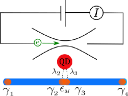
Figure 1: Schematic setup of probing the non-Abelian fusion of a pair of MZMs, say, $\gamma_{2}$ and $\gamma_{3}$, from different Majorana pairs with parities (e.g. even parity) being defined in advance. Based on the fusion rule $\gamma\times\gamma=I+\psi$, the fused MZMs would yield probabilistic outcomes of vacuum $I$ and a regular fermion $\psi$. A quantum dot is introduced to couple to the fusing MZMs for probing the fusion outcomes, and a nearby point-contact detector is introduced to detect the charge occupation of the quantum dot.

In practice, demonstrating nontrivial fusion of MZMs should require preparation of initial pair states of MZMs with definite fermion parities and nonadiabatic moving when bringing the MZMs together to fuse. In this work, along the line proposed in Ref. NC22 (as schematically shown here in Fig. 1), we consider fusing a pair of MZMs from two topological superconducting (TSC) wires (each wire accommodating two MZMs at the ends). This model setup can correspond to the platform of mini-gate controlled planar Josephson junctions RenN19 ; RenP19 . The two TSC segments can be formed from a single junction wire, by making them separated by a topologically trivial segment, via gating technology. A quantum dot is introduced to couple to the central part of the coupled wires, for use of probing the fusion outcomes when bringing the MZMs together to fuse at the central part. Moreover, a nearby point-contact (PC) detector is introduced to detect the charge occupation of the quantum dot. All the ingredients in this proposal are within the reach of nowadays state-of-the-art experiments NC22 . For fusion experiments based on this proposal, one may encounter some practical complexities, such as the interplay of charge fluctuations in the quantum dot caused by the two fusion outcomes, which is relevant to the control of the dot energy level and its coupling strengths to the MZMs, and the effect on the dot occupation pattern caused by the speed of fusion and coupling of the MZMs to the quantum dot. Detection schemes accounting for these issues will be analyzed in this work, and are expected to be useful for future experiments.

Setup and Basic Consideration

.— The setup proposed in Ref. NC22 can be modeled as Fig. 1, where the two TSC quantum wires are formed by interrupting a single TSC wire at the center via mini-gate-voltage control. For each TSC wire, a pair of MZMs are emergent at the ends, i.e., ($\gamma_{1},\gamma_{2}$) in the left wire and ($\gamma_{3},\gamma_{4}$) in the right wire. The coupling between the central modes $\gamma_{2}$ and $\gamma_{3}$ is described by $H^{\prime}_{M}=i\epsilon_{M}\gamma_{2}\gamma_{3}$, with the coupling energy $\epsilon_{M}$ changeable when $\gamma_{2}$ and $\gamma_{3}$ are separated away in space by mini-gate-voltage control.

Most naturally, one can combine ($\gamma_{1},\gamma_{2}$) as a regular fermion $f_{12}$ with occupation $n_{12}=0$ or 1, and ($\gamma_{3},\gamma_{4}$) as another regular fermion $f_{34}$ with occupation $n_{34}=0$ or 1. For fusion experiment, one can prepare the specific initial state $|0_{12}0_{34}\rangle$ as proposed in Ref. NC22 . That is, by means of mini-gate-voltage control, move $\gamma_{2}$ and $\gamma_{3}$ to the ends of the two wires, close to $\gamma_{1}$ and $\gamma_{4}$, respectively; then, empty the possible occupations of the regular fermions $f_{12}$ and $f_{34}$ by introducing tunnel-coupled side quantum dots and modulating the dot energies (while the quantum dots are also tunnel-coupled to outside reservoirs). Starting with $|0_{12}0_{34}\rangle$, consider simultaneously moving $\gamma_{2}$ and $\gamma_{3}$ from the two terminal sides back to the central part to fuse (to couple each other such that $\epsilon_{M}\neq 0$), as shown in Fig. 1. For the final state, in the representation of $n_{12}$ and $n_{34}$ occupations, it is still $|0_{12}0_{34}\rangle$. However, in the representation of $n_{23}$ and $n_{14}$, i.e., the occupations of the regular fermions $f_{23}$ and $f_{14}$ associated with the Majorana pairs ($\gamma_{2},\gamma_{3}$) and ($\gamma_{1},\gamma_{4}$), we can reexpress this state as (for derivation of this transformation rule, or the so-called fusion rule, see Appendix A)

$$|0_{12}0_{34}\rangle=\frac{1}{\sqrt{2}}(|0_{23}0_{14}\rangle+i|1_{23}1_{14}\rangle)\,.$$ (2)

We find that, in the new representation, the occupation of the $f_{23}$ fermion can be empty or occupied, i.e., $|0_{23}\rangle$ or $|1_{23}\rangle$. This is nothing but the two possible outcomes $I$ and $\psi$ of the nontrivial fusion of Ising anyons, as shown by Eq. (1).

The fusion coupling between the Majorana modes $\gamma_{2}$ and $\gamma_{3}$ would lift the energy degeneracy of the states $|0_{23}\rangle$ and $|1_{23}\rangle$, thus allowing to identify the fusion outcomes $I$ and $\psi$. Following Ref. NC22 , we consider to introduce a nearby quantum dot (QD) to couple to the central segment of the quantum wire, as shown in Fig. 1, where the Majorana modes $\gamma_{2}$ and $\gamma_{3}$ are located. The QD is assumed to have a single relevant energy level, described by $H_{D}=\epsilon_{D}d^{\dagger}d$. We thus expect different charge occupation patterns of the QD, for the different fusion outcomes $I$ and $\psi$. In this context, it would be more convenient to describe the coupling between $(\gamma_{2},\gamma_{3})$ and the QD using the regular fermion $f_{23}$ picture, as follows

$$H^{\prime}_{DF}=(\lambda_{N}d^{\dagger}f_{23}+\lambda_{A}d^{\dagger}f_{23}^{\dagger})+{\rm h.c.}\,.$$ (3)

Here we have used the definition $f_{23}=(\gamma_{2}+i\gamma_{3})/2$. Physically, the first term describes the usual normal tunneling process and the second term describes the Andreev process owing to Cooper pair splitting and recombination. The coupling amplitudes are associated with the couplings of $\gamma_{2}$ and $\gamma_{3}$ to the QD, say, $\lambda_{2}$ and $\lambda_{3}$ as shown in Fig. 1, as $\lambda_{N,A}=\lambda_{2}\pm i\lambda_{3}$.

Also following the proposal of Ref. NC22 , the charge fluctuation in the quantum dot (occupied or unoccupied) is measured by a point-contact (PC) detector, as schematically shown in Fig. 1. PC detectors with sensitivity at single electron level have been experimentally demonstrated and broadly applied in practice Ens06 ; Fuj06 ; Guo13 ; Guo15 . Actually, the measurement dynamics of a charge qubit by a PC detector has been a long standing theoretical problem and has attracted intensive interest in the community of quantum and mesoscopic physics Kor01 ; Mil01 ; Li05 ; Opp20 . In this work, we will perform real-time simulations for probing the non-Abelian fusion of a pair of MZMs. In particular, within the scheme of continuous quantum weak measurement, we will carry out results of individual quantum trajectories and power spectrum of the measurement currents. The characteristic frequencies in the power spectrum indicate the quantum oscillations of charge transfer associated with the two outcomes of fusion. The coexistence of two characteristic frequencies should be a promising evidence for the non-Abelian fusion of MZMs.

QD occupations caused by the two fusion outcomes

.— Let us consider first the detection scheme of switching on the coupling of the QD to the Majorana modes $\gamma_{2}$ and $\gamma_{3}$, after their fusion from the deterministic initial state $|0_{12}0_{34}\rangle$. This can be realized by initially setting the QD energy level much higher than the final coupling energy $\epsilon_{M}$ between $\gamma_{2}$ and $\gamma_{3}$. Then, during the moving and fusion process, the QD level is effectively decoupled with $\gamma_{2}$ and $\gamma_{3}$, owing to the large mismatch of energies. After fusion, switch on the coupling by lowering the QD energy level such that $\epsilon_{D}=\epsilon_{M}$.

For this scheme, the time dependent charge occupation in the dot is shown in Fig. 2 (the result of the green curve). To understand this result, we should notice the coexistence of two channels of charge transfer oscillations between the QD and the MZMs $\gamma_{2}$ and $\gamma_{3}$. One channel is governed by normal tunneling between the states $|1_{23}0_{d}\rangle$ and $|0_{23}1_{d}\rangle$, resulting in a quantum oscillation state as $\alpha_{N}(t)|1_{23}0_{d}\rangle+\beta_{N}(t)|0_{23}1_{d}\rangle$, with the dot occupation probability $p_{d}^{(N)}(t)=|\beta_{N}(t)|^{2}$ plotted in Fig. 2 by the full Rabi-type oscillating red curve. The other channel is governed by the Andreev process between $|0_{23}0_{d}\rangle$ and $|1_{23}1_{d}\rangle$, resulting in a quantum oscillation given by $\alpha_{A}(t)|0_{23}0_{d}\rangle+\beta_{A}(t)|1_{23}1_{d}\rangle$, with the dot occupation probability $p_{d}^{(A)}(t)=|\beta_{A}(t)|^{2}$ plotted in Fig. 2 by the smaller amplitude blue curve. These two channels are independent to each other. Thus the electron occupation in the dot is simply an equal probability weighted sum, based on Eq. (2), as

$$p_{d}(t)=\left[|\beta_{N}(t)|^{2}+|\beta_{A}(t)|^{2}\right]/2\,.$$ (4)

Actually, the quantum oscillations in the two channels have simple analytic solutions, with dot occupation probabilities given by

$$|\beta_{N,A}(t)|^{2}=\left(|\lambda_{N,A}|^{2}/\Omega_{N,A}^{2}\right)\sin^{2}\left(\Omega_{N,A}t\right)\,,$$ (5)

where $\Omega_{N,A}=\sqrt{\Delta_{N,A}^{2}+|\lambda_{N,A}|^{2}}$ and $\Delta_{N,A}=|\epsilon_{D}\mp\epsilon_{M}|/2$. We then understand that, when $\epsilon_{D}\simeq\epsilon_{M}>>|\lambda_{N,A}|$, the quantum oscillation associated with the fusion outcome $\psi$ is dominant, while the Andreev process following the $I$ outcome is largely suppressed. However, viewing that the coupling energy $\epsilon_{M}$ between $\gamma_{2}$ and $\gamma_{3}$ is small (might be comparable with $\lambda_{2}$ and $\lambda_{3}$ in practice, see Fig. 1), one may encounter the complexity that both channels coexist during detection of the charge variations in the quantum dot, having thus the result as shown in Fig. 2 by the green curve.

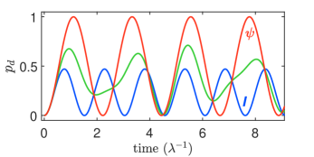
Figure 2: Dot occupation probability $p_{d}$ (green curve) associated with the detection scheme of sudden coupling of the MZMs after fusion to the probing QD. According to the fusion rule, Eq. (2), $p_{d}$ is half of the sum of $p_{d}^{(N)}$ (red curve, labeled by $\psi$) and $p_{d}^{(A)}$ (blue curve, labeled by $I$). The meaning of $p_{d}^{(N)}$ and $p_{d}^{(A)}$ is referred to the main text. Parameters are assumed as $\lambda_{2}=\lambda_{3}=\lambda=1$, and $\epsilon_{D}=\epsilon_{M}=1.5$. In this work, we use the arbitrary system of units, taking $\lambda$ as the unit of energy and $\lambda^{-1}$ as the unit of time.

Next, let us consider an alternative detection scheme of gradually coupling the QD with the Majorana modes $\gamma_{2}$ and $\gamma_{3}$. The initial state preparation and moving of the Majorana modes $\gamma_{2}$ and $\gamma_{3}$ are the same as above (the first scheme). However, we consider now initially setting the QD level in resonance with the final Majorana coupling energy, i.e., $\epsilon_{D}=\epsilon_{M}$. Then, in this scheme, modulation of the QD energy level after Majorana fusion is not needed. When $\gamma_{2}$ and $\gamma_{3}$ are somehow slowly brought to close to each other, they also couple to the QD gradually. We may model the gradual coupling as follows

$$\lambda_{2}=\lambda_{3}=\lambda\left[\frac{t}{\tau}\Theta(1-\frac{t}{\tau})+\Theta(\frac{t}{\tau}-1)\right]\,,$$

$$\epsilon_{23}=\epsilon_{M}\left[\frac{t}{\tau}\Theta(1-\frac{t}{\tau})+\Theta(\frac{t}{\tau}-1)\right]\,,$$ (6)

where $\Theta(\cdots)$ is the step function. In this simple model, $\tau$ is introduced to characterize the speed of moving $\gamma_{2}$ and $\gamma_{3}$. Here we assume that the coupling of $\gamma_{2}$ and $\gamma_{3}$ to the QD (nonzero $\lambda_{2}$ and $\lambda_{3}$) and the coupling between them (nonzero $\epsilon_{23}$) are started at same time. We also use it as the initial time for latter state evolution, which is associated with the fusion and detection. Before $\gamma_{2}$, $\gamma_{3}$ and the QD start to couple to each other, the moving of $\gamma_{2}$ and $\gamma_{3}$ can be performed at different speed (faster speed). However, the moving should satisfy the adiabatic condition determined by the energy gap of the TSC wire, which is much larger than the coupling energies $\epsilon_{M}$, $\lambda_{2}$ and $\lambda_{3}$, and the dot energy $\epsilon_{D}$. We may remark that the modeling, in terms of Eq. (Probing the non-Abelian fusion of a pair of Majorana zero modes), might not be very accurate, but it captures the underlying physics and can predict valid behavior of electron occupation in the quantum dot, in comparison with more accurate simulation based on the more realistic lattice model.

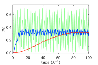
Figure 3: Dot occupation probability $p_{d}$ associated with the detection scheme of gradual fusion and coupling to the probing QD, as modeled by Eq. (Probing the non-Abelian fusion of a pair of Majorana zero modes). Results of different coupling speeds are shown for $\tau=1$ (green curve), 10 (blue curve), and 80 (red curve), respectively. Prominent feature is that the quantum oscillations tend to disappear when decreasing the speed of coupling, i.e., when approaching the adiabatic limit of switching on the coupling. Parameters are the same as assumed in Fig. 2.

In Fig. 3 we show results of different coupling speeds, which are characterized by the parameter $\tau$. For fast coupling, the result (green curve) is similar to that shown in Fig. 2. However, if decreasing the speed of coupling, the charge occupation pattern in the quantum dot becomes different. The most prominent feature is that the quantum oscillations tend to disappear (see the blue and red curves in Fig. 2). This can be understood as follows. In this scheme of fusion and detection, there exist also two charge transfer channels associated with, respectively, the fusion outcomes $I$ and $\psi$. However, in the limit of adiabatically switching on the coupling, in each channel the state will largely follow an instantaneous eigenstate. For instance, for the $\psi$-related dominant channel (governed by the normal tunneling between the states $|1_{23}0_{d}\rangle$ and $|0_{23}1_{d}\rangle$), the state can be expressed also as $\alpha_{N}(t)|1_{23}0_{d}\rangle+\beta_{N}(t)|0_{23}1_{d}\rangle$. Yet, in the adiabatic limit, the superposition coefficients in the instantaneous eigenstate do not reveal the feature of Rabi-type quantum oscillations. Actually, we can easily obtain $|\beta_{N}(t\geq\tau)|^{2}=p^{(N)}_{d}=1/2$. Similarly, for the outcome-$I$-related channel, the instantaneous eigenstate can be expressed as $\alpha_{A}(t)|0_{23}0_{d}\rangle+\beta_{A}(t)|1_{23}1_{d}\rangle$. In the adiabatic limit, $|\beta_{A}(t)|^{2}$ does not oscillate with time and, when $t\geq\tau$, we obtain

$$p^{(A)}_{d}=|\beta_{A}|^{2}=\frac{(\Omega_{A}-\epsilon_{M})^{2}}{(\Omega_{A}-\epsilon_{M})^{2}+2|\lambda|^{2}}\,.$$ (7)

Here, $\Omega_{A}=\sqrt{\epsilon^{2}_{M}+2|\lambda|^{2}}$, under the conditions $\epsilon_{D}=\epsilon_{M}$ and $\lambda_{2}=\lambda_{3}=\lambda$. Based on the fusion rule Eq. (2), we expect the overall occupation probability of an electron in the QD to be $p_{d}=(p^{(N)}_{d}+p^{(A)}_{d})/2$. Indeed, this is the asymptotic result observed in Fig. 3, in the adiabatic limit.

The QD occupations predicted in Figs. 2 and 3 can be measured by using a charge-sensitive PC-detector as shown in Fig. 1. The standard method is performing the so-called single shot projective measurement to infer the QD being occupied or not by an electron. After a large number of ensemble measurements, the occupation probability can be obtained. However, the result in Fig. 2 (the overall pattern plotted by the green curve) does not very directly reveal the coexistence of the two fusion outcomes. Also, measuring this oscillation pattern and the subsequent analyzing will be more complicated than handling the result from the adiabatic coupling as shown in Fig. 3. That is, importantly, measuring the final single constant occupation probability is much simpler than measuring the oscillation pattern in Fig. 2, while the result can more directly inform us the coexistence of the two fusion outcomes, by using the formula $p_{d}=(p^{(N)}_{d}+p^{(A)}_{d})/2$ and the result $p^{(N)}_{d}=0.5$. Therefore, the second detection scheme proposed above is expected to be useful in practice, by adiabatically switching on the probe coupling.

Continuous weak measurements.— Besides the usual strong (projective) measurements, as discussed above for measuring the QD occupation probability, continuous quantum weak measurement is an interesting and different type of choice, suitable in particular for measuring quantum oscillations. For instance, the problem of continuous weak measurement of charge qubit oscillations by a PC detector has attracted strong interest for intensive studies Kor01 ; Mil01 ; Li05 . In the following, we consider continuous weak measurement for the quantum oscillations displayed in Fig. 2 (by the green curve). Specifically, for the setup shown in Fig. 1, the PC detector is switched on (applied bias voltage) from the beginning of state evolution after fusion, owing to tunnel-coupling with the QD. The noisy output current in the PC detector can be expressed as Kor01 ; Mil01 ; Opp20

$$I_{c}(t)=n_{d,c}(t)+\frac{1}{\sqrt{4\kappa}}\,\xi(t)\,.$$ (8)

This (rescaled) expression of current is valid up to a constant factor (with current dimension). Then, the first term is simply the quantum average occupation of an electron in the quantum dot, i.e., $n_{d,c}(t)={\rm Tr}[\hat{n}_{d}\rho_{c}(t)]$, with $\rho_{c}(t)$ the PC-current-conditioned state of the measured system. The second term describes the deviation of the real noisy current from the quantum average occupation $n_{d,c}(t)$, owing to classical events of random tunneling of electrons in the PC detector. The rate parameter $\kappa$ characterizes the measurement strength and $\xi(t)$ is the Gaussian white noise. For completeness, we also present here the quantum trajectory (QT) equation for the conditional state as Mil01

$$\dot{\rho}_{c}=\mathcal{L}\rho_{c}+\sqrt{\kappa}\mathcal{H}[\hat{n}_{d}]\rho_{c}\xi(t)\,.$$ (9)

The first deterministic part is given by $\mathcal{L}\rho_{c}=-i\left[H,\rho_{c}\right]+\kappa\mathcal{D}[\hat{n}_{d}]\rho_{c}$, with the Lindblad superoperator defined as $\mathcal{D}[x]\rho_{c}=x\rho_{c}x^{\dagger}-\frac{1}{2}\{x^{\dagger}x,\rho_{c}\}$. The second noisy term stems from measurement backaction owing to information gain in the single realization of continuous weak measurement, while the superoperator is defined as $\mathcal{H}[x]\rho_{c}=x\rho_{c}+\rho_{c}x^{\dagger}-\mathrm{Tr}\left[(x+x^{\dagger})\rho_{c}\right]\rho_{c}$.

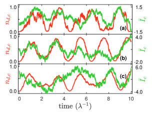
Figure 4: Quantum trajectories of continuous weak measurement, associated with the detection scheme of sudden coupling of the MZMs after fusion to the probing QD. The measurement-current-conditioned occupation $n_{d,c}(t)$ and the current $\bar{I}_{c}(t)$ (low-pass-filtered with a time window $T=1$) are shown for measurement strengths $\kappa=0.8$ in (a), 0.2 in (b), and 0.05 in (c), respectively. Other parameters are the same as in Fig. 2.

Jointly simulating the evolution of Eqs. (8) and (9) we can obtain $\rho_{c}(t)$, $n_{d,c}(t)$, and $I_{c}(t)$. From Eq. (8), we understand that the measurement current does encode the information of the QD occupation. However, owning to measurement backaction, the measurement-current-conditioned occupation $n_{d,c}(t)$ is different from the occupation probability $p_{d}(t)$ shown in Fig. 2 (in the absence of measurement). For considerably weak measurement, $n_{d,c}(t)$ should be quite close to $p_{d}(t)$, yet the noisy term in Eq. (8) will hide the informational term, thus preventing us inferring the dot occupation. In contrast, if increasing the measurement strength, the noisy term will decrease, but the measurement backaction will make $n_{d,c}(t)$ more seriously deviate from the original result $p_{d}(t)$. In Fig. 4, we show the results of $n_{d,c}(t)$ and $I_{c}(t)$, for a couple of measurement strengths. In addition to properly choosing the measurement strengths, we also applied the so-called low-pass-filtering technique. That is, we averaged the current over a sliding time window of duration $T$, $\bar{I}_{c}(t)=\frac{1}{T}\int_{t-T/2}^{t+T/2}dI_{c}(\tau)$, which gives a smoothed current for better reflecting the dot occupation. However, even after making these efforts, we find that from the noisy output current $I_{c}(t)$, it is hard to track the quantum oscillations of the QD occupation shown in Fig. 2.

Actually, in continuous weak measurements, a useful technique is extracting information from the power spectrum of the measurement currents Kor01 ; Mil01 ; Li05 . The steady-state current correlation function is obtained through the ensemble average $S_{I}(\tau)={\rm E}[I_{c}(t+\tau)I_{c}(t)]-{\rm E}[I_{c}(t+\tau)]{\rm E}[I_{c}(t)]$, at long time limit (large $t$ limit for achieving steady state). From the power spectrum, $S_{I}(\omega)=2\int^{\infty}_{-\infty}S_{I}(\tau)e^{i\omega\tau}$, one can identify the characteristic frequencies and infer thus quantum coherent oscillations inside the system under measurement. For the problem under study, the goal is to identify the quantum oscillations shown in Fig. 2, which are associated with the two fusion outcomes. Based on the result of Eq. (8), it can be proved Kor01 ; Mil01 that

$$S_{I}(\tau) = S_{d}(\tau)+\frac{1}{4\kappa}\delta(\tau)-\frac{1}{4}\,.$$ (10)

In this result, the correlation function of the dot occupation is given by $S_{d}(\tau)={\rm E}[n_{d,c}(t+\tau)n_{d,c}(t)]={\rm Tr}[{\hat{n}_{d}}e^{\mathcal{L}|\tau|}(\hat{n}_{d}\rho_{st})]$, with $\rho_{st}$ the reduced density matrix of steady state. Then, we know the structure of the current power spectrum as $S_{I}(\omega)=S_{0}+S_{d}(\omega)$, with $S_{0}$ the frequency-free background noise and $S_{d}(\omega)$ the information-contained part. Based on the master equation $\dot{\rho}={\cal L}\rho$, which is the ensemble average of Eq. (9), using the so-called quantum regression theorem we obtain

$$S_{d}^{(j)}(\omega)$$ (11)

$$= \frac{2\kappa|\lambda_{j}|^{2}(16\Delta_{j}^{2}+\kappa^{2}+4\omega^{2})}{\omega^{2}(16\Omega_{j}^{2}+\kappa^{2}-4\omega^{2})^{2}+16\kappa^{2}(2|\lambda_{j}|^{2}-\omega^{2})^{2}}.$$

Here we use $j=N,A$ to denote the two charge transfer channels, say, the Andreev process and normal tunneling, with coupling amplitudes $\lambda_{N,A}=\lambda_{2}\pm i\lambda_{3}$. Since the two channels are independent, we obtained the above results independently for each process. The overall spectrum $S_{d}(\omega)$ is the weight-averaged sum of $S_{d}^{(N)}(\omega)$ and $S_{d}^{(A)}(\omega)$, i.e., $S_{d}(\omega)=[S_{d}^{(N)}(\omega)+S_{d}^{(A)}(\omega)]/2$, owing to the fusion rule of Eq. (2). Moreover, under the condition of weak-coupling measurement, we can further approximate the result as

$$S_{d}^{(j)}(\omega)\simeq\frac{\Delta_{j}^{2}}{4\Omega_{j}^{2}}\frac{\kappa R_{j}/2}{\omega^{2}+(\kappa R_{j}/2)^{2}}$$

$$~{}+\frac{|\lambda_{j}|^{2}}{8\Omega_{j}^{2}}\frac{\frac{\kappa}{2}(1-\frac{R_{j}}{2})}{(\omega-2\Omega_{j})^{2}+[\frac{\kappa}{2}(1-\frac{R_{j}}{2})]^{2}}\,.$$ (12)

Here we have introduced $R_{j}\equiv|\lambda_{j}|^{2}/\Omega_{j}^{2}$. From this standard Lorentzian form, one can extract the characteristic frequencies $\Omega_{N}$ and $\Omega_{A}$, which reflect in essence the quantum oscillations given by Eq. (5).

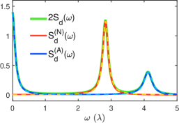
Figure 5: Characteristic frequency spectrum, $S_{d}(\omega)$, the Fourier transform of the QD-occupation correlation function, from the output currents of continuous weak measurement associated with the detection scheme of sudden coupling of the MZMs after fusion to the probing QD. Theoretically, owing to the fusion rule Eq. (2), $S_{d}(\omega)=[S_{d}^{(N)}(\omega)+S_{d}^{(A)}(\omega)]/2$, where $S_{d}^{(N)}(\omega)$ and $S_{d}^{(A)}(\omega)$ are the spectrums related to the fusion outcomes $\psi$ and $I$. Exact results of Eq. (11) are displayed by the solid-red and solid-blue curves, while approximate results of the Lorentzian form Eq. (Probing the non-Abelian fusion of a pair of Majorana zero modes) are plotted by the dashed-yellow and dashed-blue curves. $S_{d}(\omega)$ is from numerically solving the full master equation, which includes the two fusion outcomes caused charge transfer channels. Satisfactory agreement between all these results is demonstrated. The coexistence of two Lorentzian peaks (at $2\Omega_{N}$ and $2\Omega_{A}$) in $S_{d}(\omega)$ indicates the appearance of the two fusion outcomes, predicted by Eq. (1). Measurement strength $\kappa=0.4$ is assumed, while other parameters are the same as in Fig. 2.

In Fig. 5, we plot the result of $2S_{d}(\omega)$ from numerically solving the full master equation, which includes the two charger transfer channels. We find that it is indeed the sum of $S_{d}^{N}(\omega)$ and $S_{d}^{A}(\omega)$, while in this plot, for the purpose of self-consistence verification, we use their analytic solutions given by Eq. (11). We also compare the results with the approximate Lorentzian form solutions and find satisfactory agreement. Very importantly, the coexistence of two Lorentzian peaks (at $2\Omega_{N}$ and $2\Omega_{A}$) in $S_{d}(\omega)$ simply indicates the appearance of the two fusion outcomes, predicted by Eq. (1).

We may remark that, within the scheme of continuous quantum weak measurement, from its output current power spectrum $S_{I}(\omega)$ to infer the intrinsic quantum oscillations is a very useful scheme, which is much simpler than the ensemble single shot projective measurements of the dot occupation, in order to obtain the probabilities as shown in Figs. 2 and 3. This type of technique has been analyzed in detail in the context of charge-qubit measurements Kor01 ; Mil01 ; Li05 . The present proposal is an extension along this line, hopefully to be employed to identify the non-Abelian fusion of MZMs, through the two different characteristic frequencies of quantum oscillations, which are associated with the two fusion outcomes.

Summary

.— We have analyzed two schemes of detecting the nontrivial fusion of a pair of MZMs. The two possible stochastic fusion outcomes reflect the non-Abalian statistics nature of the MZMs, whose experimental demonstration will be a milestone for ultimately identifying the MZMs and paving the way to topological quantum computation. One scheme, the most natural choice, is to switch on sudden coupling of the fused MZMs to the probing QD, with the subsequent QD oscillating occupation being monitored by a PC detection in terms of continuous weak measurement. From the power spectrum of the measurement currents, one can identify two characteristic frequencies of quantum oscillations and infer thus the two fusion outcomes of the pair of MZMs. The other scheme is to switch on, almost adiabatically, gradual fusion coupling between the MZMs and their coupling to the probing QD. This type of detection scheme will result in the QD occupation not oscillating with time, thus allowing a simpler way to measure the single value of the QD occupation probability and using it to infer the two outcomes of nontrivial fusion. We expect that both detection schemes analyzed in this work can be useful for future fusion experiments.

Acknowledgements.

— This work was supported by the NNSF of China (Grants No. 11974011 and No. 11904261).

Appendix A Derivation of the Fusion Rule

In this Appendix let us prove the following transformation rule (fusion rule):

$$|0_{12}0_{34}\rangle=\frac{1}{\sqrt{2}}(|0_{23}0_{14}\rangle+i|1_{23}1_{14}\rangle)\,.$$

Under the constraint of fermion parity, in general, we may first construct the transformation ansatz as $|0_{12}0_{34}\rangle=a|0_{23}0_{14}\rangle+b|1_{23}1_{14}\rangle)$. Then, we express the operator $f_{12}=(\gamma_{1}+i\gamma_{2})/2$ in terms of the regular fermion operators $f_{14}$ and $f_{23}$ as

$$f_{12}=\frac{1}{2}\left(f_{14}+f^{\dagger}_{14}+if_{23}+if^{\dagger}_{23}\right)\,.$$ (13)

This result is obtained by simply associating the Majorana fermions $\gamma_{1}$ and $\gamma_{4}$ with the regular fermion $f_{14}$, and $\gamma_{2}$ and $\gamma_{3}$ with $f_{23}$, respectively. Thus we have $\gamma_{1}=f_{14}+f^{\dagger}_{14}$ and $\gamma_{2}=f_{23}+f^{\dagger}_{23}$. Further, acting the annihilation operator $f_{12}$ on both sides of the ansatz equation, we have

$$0=a(|0_{23}1_{14}\rangle+i|1_{23}0_{14}\rangle)$$

$$~{}~{}~{}+b(i|0_{23}1_{14}\rangle-|1_{23}0_{14}\rangle)\,.$$ (14)

During the algebra, one should notice the difference of a minus sign between $f_{23}|1_{23}1_{14}\rangle=|0_{23}1_{14}\rangle$ and $f_{14}|1_{23}1_{14}\rangle=-|1_{23}0_{14}\rangle$. From this result, we obtain $ia-b=0$ and $a=1/\sqrt{2}$, which finishes the proof of the above formula of transformation. Applying the same method outlined above, one can carry out all the transformation formulas between the two sets of basis states, $|n_{12}n_{34}\rangle$ and $|n_{23}n_{14}\rangle$.

References

- (1) A. Y. Kitaev, Unpaired Majorana fermions in quantum wires, Phys. Usp. 44, 131 (2001).
- (2) A. Y. Kitaev, Fault-tolerant quantum computation by anyons, Ann. Phys. 303, 2 (2003).
- (3) C. Nayak, S. H. Simon, A. Stern, M. Freedman, and S. D. Sarma, Non-Abelian anyons and topological quantum computation, Rev. Mod. Phys. 80, 1083 (2008).
- (4) B. M. Terhal, Quantum error correction for quantum memories, Rev. Mod. Phys. 87, 307-346 (2015).
- (5) S. D. Sarma, M. Freedman, and C. Nayak, Majorana zero modes and topological quantum computation, Quantum Inf. 1, 15001 (2015).
- (6) Y. Oreg and F. von Oppen, Majorana Zero Modes in Networks of Cooper-pair Boxes: Topologically Ordered States and Topological Quantum Computation, Annu. Rev. Condens. Matter Phys. 11, 397 (2020).
- (7) G. Li, S. Zhu, P. Fan, L. Cao, and H.-J. Gao, Exploring Majorana zero modes in iron-based superconductors, Chin. Phys. B 31, 080301 (2022).
- (8) J. Alicea, Y. Oreg, G. Refael, F. von Oppen, and M. Fisher, Non-Abelian statistics and topological quantum information processing in 1D wire networks, Nat. Phys. 7, 412 (2011).
- (9) B. I. Halperin, Y. Oreg, A. Stern, G. Refael, J. Alicea, and F. von Oppen, Adiabatic manipulations of Majorana fermions in a three-dimensional network of quantum wires, Phys. Rev. B 85, 144501 (2012).
- (10) F. Harper, A. Pushp, and R. Roy, Majorana braiding in realistic nanowire Y-junctions and tuning forks, Phys. Rev. Research 1, 033207 (2019).
- (11) C. Tutschku, R. W. Reinthaler, C. Lei, A. H. MacDonald, and E. M. Hankiewicz, Majorana-based quantum computing in nanowire devices, Phys. Rev. B 102, 125407 (2020).
- (12) D. Aasen, M. Hell, R. Mishmash, A. Higginbotham, J. Danon, M. Leijnse, T. Jespersen, J. Folk, C. Marcus, K. Flensberg, and J. Alicea, Milestones Toward Majorana-Based Quantum Computing, Phys. Rev. X 6, 031016 (2016).
- (13) C. W. J. Beenakker, Search for non-Abelian Majorana braiding statistics in superconductors, SciPost Phys. Lect. Notes 15 (2020).
- (14) T. Zhou, M. C. Dartiailh, K. Sardashti, J. E. Han, A. Matos-Abiague, J. Shabani, and I. Z̆utić, Fusion of Majorana bound states with mini-gate control in two-dimensional systems, Nat. Commun. 13, 1738 (2022).
- (15) R. S. Souto, and M. Leijnse, Fusion rules in a Majorana single-charge transistor, SciPost Phys. 12, 161 (2022).
- (16) T. Zhou, M. C. Dartiailh, W. Mayer, J. E. Han, A. Matos-Abiague, J. Shabani, and I. Z̆utić, Phase Control of Majorana Bound States in a Topological X Junction, Phys. Rev. Lett. 124, 137001 (2020).
- (17) C.-X. Liu, H. Pan, F. Setiawan, M. Wimmer, and J. D. Sau, Fusion protocol for Majorana modes in coupled quantum dots, Phys. Rev. B 108, 085437 (2023).
- (18) H. Ren, F. Pientka, S. Hart, A. T. Pierce, M. Kosowsky, L. Lunczer, R. Schlereth, B. Scharf, E. M. Hankiewicz, L. W. Molenkamp, B. I. Halperin, and A. Yacoby. Topological Superconductivity in a Phase-Controlled Josephson Junction, Nature 569, 93 (2019).
- (19) B. Scharf, F. Pientka, H. Ren, A. Yacoby, and E. M. Hankiewicz, Tuning topological superconductivity in phase-controlled Josephson junctions with Rashba and Dresselhaus spin-orbit coupling, Phys. Rev. B 99, 214503 (2019).
- (20) S. Gustavsson, R. Leturcq, B. Simovic, R. Schleser, T. Ihn, P. Studerus, K. Ensslin, D. C. Driscoll, and A. C. Gossard, Counting Statistics of Single Electron Transport in a Quantum Dot, Phys. Rev. Lett. 96, 076605 (2006).
- (21) T. Fujisawa, T. Hayashi, R. Tomita, and Y. Hirayama, Bidirectional Counting of Single Electrons, Science 312, 1634 (2006).
- (22) G. Cao, H. O. Li, T. Tu, L. Wang, C. Zhou, M. Xiao, G. C. Guo, H. W. Jiang, and G. P. Guo, Ultrafast universal quantum control of a quantum dot charge qubit using Landau-Zener-Stückelberg interference, Nat. Commun. 4, 1401 (2013).
- (23) H. O. Li, G. Cao, G. D. Yu, M. Xiao, G. C. Guo, H. W. Jiang, and G. P. Guo, Conditional rotation of two strongly coupled semiconductor charge qubits, Nat. Commun. 6, 7681 (2015).
- (24) A. N. Korotkov, Output spectrum of a detector measuring quantum oscillations, Phys. Rev. B 63, 085312 (2001).
- (25) H. S. Goan and G. J. Milburn, Dynamics of a mesoscopic qubit under continuous quantum measurement, Phys. Rev. A 96, 033804 (2017).
- (26) X. Q. Li, P. Cui, and Y. J. Yan, Spontaneous Relaxation of a Charge Qubit under Electrical Measurement, Phys. Rev. Lett. 94, 066803 (2005).
- (27) J. F. Steiner and F. von Oppen, Readout of Majorana qubits, Phys. Rev. Research 2, 033255 (2020).