Upper branch thermal Hall effect in quantum paramagnets
Bowen Ma2,3Z. D. Wang2Gang Chen1,2,3,gangchen.physics@gmail.com1International Center for Quantum Materials,
School of Physics, Peking University, Beijing 100871, China
2Department of Physics and HK Institute of Quantum Science & Technology,
The University of Hong Kong, Pokfulam Road, Hong Kong, China
3The University of Hong Kong Shenzhen Institute of Research and Innovation,
Shenzhen 518057, China
Abstract
Inspired by the persistent thermal Hall effects at finite temperatures in various quantum
paramagnets, we explore the origin of the thermal Hall effects from the perspective
of the upper branch parts by invoking the dispersive and twisted crystal field excitations.
It is shown that, the upper branches of the local energy levels could hybridize and form
the dispersive bands. The observation is that, upon the time-reversal symmetry breaking
by the magnetic fields, these upper branch bands could acquire a Berry curvature distribution
and contribute to the thermal Hall effect in the paramagnetic regime. As a proof of principle,
we consider the setting on the kagomé lattice with one ground state singlet and an excited
doublet, and show this is indeed possible. We expect this effect to be universal and
has no strong connection with the underlying lattice. Although the thermal Hall signal
can be contributed from other sources such as phonons and their scattering in the actual materials,
we discuss the application to the Mott systems with the large local Hilbert spaces.
Recently thermal Hall transports are widely used to explore the properties of the
elementary excitations in correlated quantum materials.
In the Mott insulating systems where the relevant excitations are charge neutral,
the thermal Hall effect plays an important role in deciphering the Berry curvature
properties of the excitations [1].
For spin liquids, the half-quantized thermal Hall conductivity is one smoking-gun result
for the gapped Kitaev spin liquid with the chiral Majorana edge mode [2],
and might have been observed in -RuCl3 [3, 4].
The thermal Hall effects could reflect the intrinsic matter-gauge coupling and
the Berry curvature properties of the emergent exotic quasiparticles in different spin liquids.
As a probe of the magnetic excitations, the thermal Hall effect is found to be useful
in more conventional magnets. The magnon thermal Hall
effects [5, 6, 7, 8, 9]
were widely studied in many ordered magnets. In a class of magnets known as
“dimerized magnets” where the ground state is approximately given as the product
of the spin-singlet dimers on the bonds with stronger exchanges,
the spin-triplet excitations, known as “triplons”, can propagate via the inter-dimer couplings
and form the triplon bands. These triplon bands can acquire the non-trivial Berry curvatures
and even finite Chern numbers once the anisotropic interaction such as the Dzyaloshinskii-Moriya
interaction is introduced [10, 11].
This leads to interesting behaviors in the triplon thermal Hall effect.
The thermal Hall conductivity has been measured in several visible quantum magnets
such as Tb2Ti2O7 [12], Pr2Zr2O7 [13],
Pr2Ir2O7 [14] and Na2Co2TeO6 [15, 16].
One common feature of these quantum magnets is that, due to the combination
of the crystal electric field (CEF) and the spin-orbit coupling (SOC),
the magnetic ions have a relatively large local physical Hilbert space
with a series of local energy levels [17].
We take the well-known compound Tb2Ti2O7
for example [18, 19, 12].
Via the SOC, the Tb3+ ion has a local moment.
The 13-fold degeneracy is further split by the CEF into multiple singlets
and doublets. As the thermal Hall transport in Tb2Ti2O7 was
measured up to 142 K and 10 T [12],
at this temperature scale, the second excited doublet (at 1.41 meV) has already been
thermally activated. The CEF multiplets could then make a significant impact
on the physics of those quantum magnets [20]. In addition,
the CEF levels at 10-20 meV would be thermally populated.
The 10 T magnetic field reorganizes these CEF states and splits the doublets.
For the activated CEF states, the 10 T field could create a Zeeman splitting of about 20-40 K.
The previous work that studies the monopole thermal Hall effect [21]
from the ground state doublets in the quantum ice regime [19]
certainly cannot be extended to such high temperatures and large magnetic field regimes.
Thus, these two ingredients, i.e. the thermal activation and the field
splitting/hybridization of the CEF states, indicate that,
one should seriously consider the involvement of these excited
CEF states in thermal transports. Similar physics should
generally occur in other quantum magnets with a large local Hilbert space.
This aspect is quite different from the cuprate system where the local Hilbert space
for a large range of energy scale is a spin-1/2 local moment from the electrons
and a large thermal Hall signal was observed [22, 23].
Remarkably, if one views these CEF excitations as the generalized “triplons”
with respect to the CEF ground state, this view bridges
this series of quantum magnets with the dimerized magnets.
One immediate outcome is that, these generalized “triplons”,
similar to the topological excitations in excitonic magnets [24],
should in principle possess the Berry curvatures in the magnetic field
and contribute to the thermal Hall conductivity at the relevant temperature regime.
In Ref. [25], the upper branch magnetism
from the excited CEF states was understood when the CEF gap is comparable
to the exchange interaction between the CEF states of neighboring sites.
Thus, the thermal Hall effect from the generalized triplons is dubbed
“upper branch thermal Hall effect”.
Since the upper branch thermal Hall effect arises from the CEF states and their interactions that
depend on the CEF wavefunctions and lattice symmetries, the underlying lattice is needed
but does not play a significant role in the physics. Thus, we simply consider the setting
on a kagomé lattice as shown in Fig. 1.
This can either be established by applying the [111] magnetic field
on the pyrochlore magnets, or naturally occurs
in the tripod kagomé magnets [26, 27].
Since we are mostly concerned about the excited CEF states, to simplify the problem,
we assume the CEF ground state is a singlet and the excited CEF states form a doublet.
The three states of the local moment are then described by an effective spin with
an onsite anisotropic term and ,
where is defined along the local coordinate system for each sublattice.
The spin-1 moment differs from the pseudospin-1/2 moment that is often used to describe Kramers
or non-Kramers doublets. In our design, the lower singlet corresponds to ,
and the upper doublet correspond to . If the lower singlet and the upper
doublet are connected by the ladder operator of the original operators,
all the components of are odd under time reversal.
For the spin interaction, we consider an exchange model that is quadratic
in the effective spin-1 components. The effective spin Hamiltonian is written
as
(1)
where is the Dzyaloshinskii-Moriya (DM) vector [28, 29]
for the bond with both in-plane component and out-of-plane component in general [30].
Although the Zeeman coupling could involve all the spin components,
only the Zeeman coupling to the local component is considered for simplicity.
Moreover, more complicated spin interactions such as the pseudo-dipolar interaction
and higher-order spin interactions could be present. This kind of interaction between the upper
doublets of neighboring sites have the form of a four-spin interaction [25].
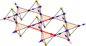
Figure 1:
(a) The tripod kagomé lattice with the effective spins on the red sites.
The blue arrows denote the local Ising axes.
The red vectors are the basis vectors
and .
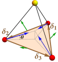
(b) The tripod unit cell. The Ising axes have a canting angle with the kagomé plane.
The green arrow normal to each bond shows the DM vectors with in-plane component
and out-of-plane component . The neighboring bonds are ,
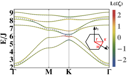
, and .Figure 2: The band dispersion of the doublet excitations from the linear flavor-wave theory.
We set , , ,
and for the solid (dashed) lines.
The color of the solid line shows the non-zero Berry curvature [30] in the log scale .
The inset shows the hexagonal Brillouin zone.
In the strong anisotropic limit with , the ground state is a simple
quantum paramagnet with . With the exchange interaction,
the many-body ground state depletes a bit from , which is analogous
to the depletion of superfluid weight in the Bose-Einstein condensation of interacting
bosons. The excited doublets form the dispersive bands.
The picture does not alter much in the
presence of external magnetic fields. As the ground state is paramagnetic without ordering,
the usual Holstein-Primakoff boson representation is not suitable to describe the excitations.
Instead, we regard
as three different flavors [31, 32] in the spirit of the SU(3) flavors,
and invoke a flavor representation of as [33, 30],
(5)
where spans a local coordinate for site .
For the quantum paramagnet here, the boson operators and
( and ) create (annihilate) a state with a “magnetic flavor”
and , respectively.
Due to the noncollinearity of the Ising axes of the three sublattices,
one needs to rotate the spin operators in Eq. (1) into the local coordinate
for different sites [34, 35],
and this generates the pairing of the flavor bosons.
Therefore, after the Fourier transform, the Hamiltonian Eq. (1)
needs to be written in a Bogoliubov-de Gennes (BdG) form [30] as
with
(6)
and
(7)
The dispersion of the flavor-wave excitations can be determined as the positive eigenvalues of
[34, 36],
where
with the Pauli matrix and the identity matrix. In Fig. 2,
we depict the representative dispersions in the quantum paramagnetic phase.
When , the bands are separated from each other.
If the band bottom touches zero energy, the bosons begin to condensate [30],
and the system develops a corresponding magnetic order [33].
To avoid that, we work in the regime with such that the quantum
paramagnet remains stable throughout.
In magnetically ordered systems,
the DM interaction or/and the noncollinear spin configuration could give
rise to topological magnons with non-zero Chern numbers [37, 38, 39, 7].
With the DM interactions and/or the noncollinear Ising axes in the current model,
the Berry curvature of the flavor-wave excitation in the quantum paramagnet
is also expected to be non-zero. In the case of the bosonic BdG Hamiltonian,
the wavefunction of the -th band is determined by the eigen-equation
.
The corresponding Berry connection
and Berry curvature is then defined as [9, 30],
(8)
In two-dimensional systems, the first Chern number can then be calculated
by integrating the -component of over the Brillouin zone as
(9)
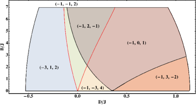
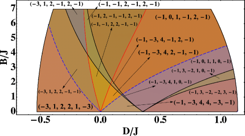
Figure 3: Diagram of Chern numbers distributions for the lower three bands.
The Chern numbers are listed from bottom to top. We set
, , , and .
The red solid and black thick lines denote the band touching
and the Chern number change at high-symmetry points and
, respectively.
The outer boundary of the quantum paramagnet is determined
when the band bottom touches zero energy at .
The general analysis of the band topology with an arbitrary choice of
parameters is unnecessary for our purpose. Without loss of much generality,
we consider a simple case where the Ising axes
are all perpendicular to the kagomé plane, and DM vectors only have
out-of-plane component as .
With this simplification, if we perform a basis transformation that
and ,
the Hamiltonian can then be written as
(10)
with
(11)
where ,,
and .
The Hamiltonian Eq. (10) is an analog of a phononic system on the kagomé lattice
with a mass and a dynamical matrix .
It can be shown [30] that the wavefunction of this “phononic” Hamiltonian remains unchanged
when and the topological properties are actually determined by .
Interestingly, is topologically equivalent to the chiral spin Hamiltonian [40] or topological magnonic Hamiltonian [6] on kagomé lattice, where the inequivalence between the honeycomb plaquette and the triangular plaquette leads to a non-zero -flux. Therefore, there is a SU(3)SU(3) band topology where the Chern numbers of the three bands with flavor are determined by a SU(3) structure [41] as from bottom to top.
In a more general situation with non-collinear Ising axes, we choose
and assume the system further respects a point group symmetry
that is inherited from the parent pyrochlore lattice so that .
After numerically computing the band Chern number in the discretized
momentum space [42], we obtain a topological phase diagram for the lower three bands shown in Fig. 3. The full diagram for all six bands can be found in the supplement [30]. We find that, due to the mixing of the two flavors in the global coordinate, the SU(3)SU(3) topology is enriched with varying intrinsic couplings as well as the external magnetic field.
From the analytical calculation and numerical study above, we can see that non-trivial Berry physics of the excited doublets in our model originates from the non-cancellation of the flux in the kagomé lattice, and thus we believe that similar non-trivial topology for even more general multiplet excitations will also occur in various lattices with inequivalent plaquettes such as honeycomb [43], checker-board [44, 45] and bulk [33] or thin-filmed [46] pyrochlore lattices.
Semiclassically, with the finite Berry curvature,
the wave-packet of the excitations will experience an anomalous velocity from
as [47, 48],
(12)
where is the packet center of the -th wavefunction.
If a longitudinal temperature gradient is applied across the material,
the transverse motion of the excitations from the anomalous velocity term will lead to some Hall-like transport signals. In the case of thermal Hall effects, the excitations carrying different energies will experience different anomalous velocities, and thus lead to a transverse temperature difference. From the theoretical side, the associated thermal Hall conductivity
of bosonic excitations can be derived from linear response theory as [49, 50],
(13)
where , Li
is the polylogarithm function, is the average temperature,
is the volume of the material, and
is the Bose-Einstein distribution.
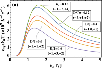
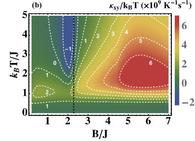
In Fig. 4(a), we show the dependence of
on the temperature with different DM interactions .
As we can infer from Eq. (13), because of the distribution function,
the Berry curvature from lower bands contributes more to the thermal Hall conductivity.
Therefore, the thermal Hall conductivity is large when ,
as the two lowest bands both have negative Chern numbers.
Meanwhile, the thermal Hall conductivity is small in the case of ,
where the second lowest band with a large positive Chern number
suppresses the contribution of negative Berry curvature from the lowest band.
Besides, if the temperature is getting higher, the occupations of the excitations
in all six bands become more equally populated, and thus
goes closer to zero owing to the fact that .
Figure 4: The thermal Hall conductivity with varying parameters.
We set , , and (a) with different values of
and the corresponding Chern numbers of the lower three bands labeled in the plot; (b)
with the white numbers and dashed lines denoting the values of (in unit of Ks-1).
The black dashed line shows the critical field
where the Chern numbers of the lower three bands change between and ,
resulting in a sign change of the thermal conductivity.
In experiments, the DM interaction is usually not tunable, and we thus depict a density plot of with respect to the magnetic field and the temperature in Fig. 4(b). With the lattice constant 10 Å of Tb2Ti2O7 as an estimate for the interlayer distance , K-1s-1 gives rise to a bulk thermal Hall signal WK-2m-1, in the same order as experimental measurements [12]. Due to the change of lower-band Berry curvature, with the magnetic field increasing, when the Chern numbers of the two lowest bands change from to , there is a sign flip of the thermal Hall conductivity around the critical field (denoted as the dotted black line). It should be pointed out that the phononic or extrinsic contribution to the sign change of thermal Hall effects in paramagnets is usually not tunable by the magnetic field or can be tuned limitedly accompanied by some magnetic phase transitions [51, 52]. We expect the observation of this sign change can indicate the presence of the upper branch thermal Hall effect, while a delicate experimental design may be needed to subtract the contribution from phonons as their effects are usually within the same order [14]. As we stated in the previous section, though we obtain the above results from a specific model on the kagomé lattice, the tunable thermal Hall signal arising from the topology of the excited multiplets can generally occur in various lattices.
In this work, we have addressed the question whether applying a Zeeman field
to Mott insulators with multiple local energy levels could generate the intrinsic
thermal Hall effect solely from the magnetic excitations in the quantum paramagnetic
phase at finite temperatures. In our simple modeling, we have only considered
the lowest few CEF energy levels, which is sufficient to provide a positive answer.
In reality, the candidate Mott insulators have many such CEF energy levels,
and as the temperature increases, these CEF energy levels would be gradually
thermally activated and contribute to thermal Hall transports.
Thus, a comprehensive understanding of the thermal Hall signals
in the candidate materials requires the intrinsic components.
We expect our results to be complementary to the recent efforts
in the phonon thermal Hall effects with the non-Kramers-like doublet systems [53, 54].
The previous analysis on Pr2Ir2O7 has pointed out the resonant
phonon-pseudospin scattering where the non-Kramers pseudospin arises
from the ground state doublet of the Pr3+ ion.
The inclusion of the upper branch CEF states not only generates the intrinsic thermal Hall
sign as the upper branch thermal Hall effect,
and may induce a cascade of resonant phonon scattering with the large local Hilbert space [55].
In conventional ordered magnets, the phonon-magnon hybridization [56, 57, 58] was known to create Berry
curvature distribution for the hybridized excitations, and can also lead to non-zero magneto-phonon chirality with
thermal Hall effects [36, 59]. This effect occurs even for the trivial magnon band structure that is absent of
finite magnon Berry curvatures.
For the exciton-like flavor-wave excitation in the quantum paramagnets,
similar phonon-exciton hybridization could occur. Here the flavor-wave excitation already
develops Berry curvature distribution on its own.
Thus, the hybridization could bring more interesting aspects to the dynamical properties of the whole system.
Acknowledgments.—This work is supported by the National Science Foundation of China with Grant No. 92065203, the Ministry of Science and Technology of China with Grants No. 2021YFA1400300, and by the Research Grants Council of Hong Kong with Grant No. C6009-20G and C7012-21G.
References
Zhang et al. [2023]X.-T. Zhang, Y. H. Gao, and G. Chen, Thermal Hall effects in quantum magnets (2023), arXiv:2305.04830 [cond-mat.str-el] .
Kasahara et al. [2018]Y. Kasahara, T. Ohnishi, Y. Mizukami, O. Tanaka, S. Ma, K. Sugii, N. Kurita, H. Tanaka, J. Nasu, Y. Motome, et al., Majorana quantization and half-integer thermal quantum Hall effect in a Kitaev spin liquid, Nature 559, 227 (2018).
Yokoi et al. [2021]T. Yokoi, S. Ma, Y. Kasahara, S. Kasahara, T. Shibauchi, N. Kurita, H. Tanaka, J. Nasu, Y. Motome, C. Hickey, et al., Half-integer quantized anomalous thermal Hall effect in the Kitaev material candidate -RuCl3, Science 373, 568 (2021).
Onose et al. [2010]Y. Onose, T. Ideue, H. Katsura, Y. Shiomi, N. Nagaosa, and Y. Tokura, Observation of the magnon hall effect, Science 329, 297 (2010).
Katsura et al. [2010]H. Katsura, N. Nagaosa, and P. A. Lee, Theory of the thermal hall effect in quantum magnets, Phys. Rev. Lett. 104, 066403 (2010).
Laurell and Fiete [2018]P. Laurell and G. A. Fiete, Magnon thermal hall effect in kagome antiferromagnets with dzyaloshinskii-moriya interactions, Phys. Rev. B 98, 094419 (2018).
Neumann et al. [2022]R. R. Neumann, A. Mook, J. Henk, and I. Mertig, Thermal hall effect of magnons in collinear antiferromagnetic insulators: Signatures of magnetic and topological phase transitions, Phys. Rev. Lett. 128, 117201 (2022).
Romhányi et al. [2015]J. Romhányi, K. Penc, and R. Ganesh, Hall effect of triplons in a dimerized quantum magnet, Nature communications 6, 6805 (2015).
McClarty et al. [2017]P. A. McClarty, F. Krüger, T. Guidi, S. Parker, K. Refson, A. Parker, D. Prabhakaran, and R. Coldea, Topological triplon modes and bound states in a Shastry–Sutherland magnet, Nature Physics 13, 736 (2017).
Hirschberger et al. [2015]M. Hirschberger, J. W. Krizan, R. Cava, and N. Ong, Large thermal hall conductivity of neutral spin excitations in a frustrated quantum magnet, Science 348, 106 (2015).
Chu and Sun [2023]W. Chu and X. Sun, Low-temperature thermal Hall conductivity of Pr2Zr2O7 single crystal, arXiv preprint arXiv:2302.13300 10.48550/arXiv.2302.13300 (2023).
Uehara et al. [2022]T. Uehara, T. Ohtsuki, M. Udagawa, S. Nakatsuji, and Y. Machida, Phonon thermal hall effect in a metallic spin ice, Nature Communications 13, 4604 (2022).
Yang et al. [2022]H. Yang, C. Kim, Y. Choi, J. H. Lee, G. Lin, J. Ma, M. Kratochvílová, P. Proschek, E.-G. Moon, K. H. Lee, Y. S. Oh, and J.-G. Park, Significant thermal Hall effect in the cobalt Kitaev system , Phys. Rev. B 106, L081116 (2022).
Takeda et al. [2022]H. Takeda, J. Mai, M. Akazawa, K. Tamura, J. Yan, K. Moovendaran, K. Raju, R. Sankar, K.-Y. Choi, and M. Yamashita, Planar thermal Hall effects in the Kitaev spin liquid candidate , Phys. Rev. Res. 4, L042035 (2022).
Gardner et al. [2010]J. S. Gardner, M. J. P. Gingras, and J. E. Greedan, Magnetic pyrochlore oxides, Rev. Mod. Phys. 82, 53 (2010).
Gardner et al. [1999]J. S. Gardner, S. R. Dunsiger, B. D. Gaulin, M. J. P. Gingras, J. E. Greedan, R. F. Kiefl, M. D. Lumsden, W. A. MacFarlane, N. P. Raju, J. E. Sonier, I. Swainson, and Z. Tun, Cooperative Paramagnetism in the Geometrically Frustrated Pyrochlore Antiferromagnet , Phys. Rev. Lett. 82, 1012 (1999).
Molavian et al. [2007]H. R. Molavian, M. J. P. Gingras, and B. Canals, Dynamically Induced Frustration as a Route to a Quantum Spin Ice State in via Virtual Crystal Field Excitations and Quantum Many-Body Effects, Phys. Rev. Lett. 98, 157204 (2007).
Voleti et al. [2023]S. Voleti, F. D. Wandler, and A. Paramekanti, Impact of gapped spin-orbit excitons on low energy pseudospin exchange interactions, arXiv preprint arXiv:2303.04169 (2023).
Zhang et al. [2020a]X.-T. Zhang, Y. H. Gao, C. Liu, and G. Chen, Topological thermal Hall effect of magnetic monopoles in the pyrochlore U(1) spin liquid, Phys. Rev. Res. 2, 013066 (2020a).
Grissonnanche et al. [2019]G. Grissonnanche, A. Legros, S. Badoux, E. Lefrançois, V. Zatko, M. Lizaire, F. Laliberté, A. Gourgout, J.-S. Zhou, S. Pyon, et al., Giant thermal hall conductivity in the pseudogap phase of cuprate superconductors, Nature 571, 376 (2019).
Boulanger et al. [2020]M.-E. Boulanger, G. Grissonnanche, S. Badoux, A. Allaire, É. Lefrançois, A. Legros, A. Gourgout, M. Dion, C. Wang, X. Chen, et al., Thermal Hall conductivity in the cuprate Mott insulators Nd2CuO4 and Sr2CuO2Cl2, Nature communications 11, 5325 (2020).
Anisimov et al. [2019]P. S. Anisimov, F. Aust, G. Khaliullin, and M. Daghofer, Nontrivial Triplon Topology and Triplon Liquid in Kitaev-Heisenberg-type Excitonic Magnets, Phys. Rev. Lett. 122, 177201 (2019).
Liu et al. [2019]C. Liu, F.-Y. Li, and G. Chen, Upper branch magnetism in quantum magnets: Collapses of excited levels and emergent selection rules, Phys. Rev. B 99, 224407 (2019).
Dun et al. [2016]Z. L. Dun, J. Trinh, K. Li, M. Lee, K. W. Chen, R. Baumbach, Y. F. Hu, Y. X. Wang, E. S. Choi, B. S. Shastry, A. P. Ramirez, and H. D. Zhou, Magnetic Ground States of the Rare-Earth Tripod Kagome Lattice (), Phys. Rev. Lett. 116, 157201 (2016).
Dun et al. [2020]Z. Dun, X. Bai, J. A. M. Paddison, E. Hollingworth, N. P. Butch, C. D. Cruz, M. B. Stone, T. Hong, F. Demmel, M. Mourigal, and H. Zhou, Quantum Versus Classical Spin Fragmentation in Dipolar Kagome Ice , Phys. Rev. X 10, 031069 (2020).
[30]See supplementary materials for details on the linear flavor-wave theory, spin hamiltonian, bosonic topology, the full diagram for the six band chern numbers, and the phononic analogy of the collinear case.
Joshi et al. [1999]A. Joshi, M. Ma, F. Mila, D. N. Shi, and F. C. Zhang, Elementary excitations in magnetically ordered systems with orbital degeneracy, Phys. Rev. B 60, 6584 (1999).
Li et al. [1998]Y. Q. Li, M. Ma, D. N. Shi, and F. C. Zhang, SU(4) Theory for Spin Systems with Orbital Degeneracy, Phys. Rev. Lett. 81, 3527 (1998).
Li and Chen [2018]F.-Y. Li and G. Chen, Competing phases and topological excitations of spin-1 pyrochlore antiferromagnets, Phys. Rev. B 98, 045109 (2018).
Ma et al. [2020]B. Ma, B. Flebus, and G. A. Fiete, Longitudinal spin Seebeck effect in pyrochlore iridates with bulk and interfacial Dzyaloshinskii-Moriya interaction, Phys. Rev. B 101, 035104 (2020).
Ma and Fiete [2022]B. Ma and G. A. Fiete, Antiferromagnetic insulators with tunable magnon-polaron chern numbers induced by in-plane optical phonons, Phys. Rev. B 105, L100402 (2022).
Mook et al. [2014]A. Mook, J. Henk, and I. Mertig, Edge states in topological magnon insulators, Phys. Rev. B 90, 024412 (2014).
Kim et al. [2016]S. K. Kim, H. Ochoa, R. Zarzuela, and Y. Tserkovnyak, Realization of the haldane-kane-mele model in a system of localized spins, Phys. Rev. Lett. 117, 227201 (2016).
Ohgushi et al. [2000]K. Ohgushi, S. Murakami, and N. Nagaosa, Spin anisotropy and quantum Hall effect in the kagomé lattice: Chiral spin state based on a ferromagnet, Phys. Rev. B 62, R6065 (2000).
Barnett et al. [2012]R. Barnett, G. R. Boyd, and V. Galitski, SU(3) Spin-Orbit Coupling in Systems of Ultracold Atoms, Phys. Rev. Lett. 109, 235308 (2012).
Ganesh et al. [2011]R. Ganesh, D. N. Sheng, Y.-J. Kim, and A. Paramekanti, Quantum paramagnetic ground states on the honeycomb lattice and field-induced néel order, Phys. Rev. B 83, 144414 (2011).
Sadrzadeh et al. [2019]M. Sadrzadeh, R. Haghshenas, and A. Langari, Quantum phase diagram of the two-dimensional transverse-field ising model: Unconstrained tree tensor network and mapping analysis, Phys. Rev. B 99, 144414 (2019).
Hu et al. [2012]X. Hu, A. Rüegg, and G. A. Fiete, Topological phases in layered pyrochlore oxide thin films along the [111] direction, Phys. Rev. B 86, 235141 (2012).
Xiao et al. [2010]D. Xiao, M.-C. Chang, and Q. Niu, Berry phase effects on electronic properties, Rev. Mod. Phys. 82, 1959 (2010).
Cheng et al. [2016]R. Cheng, S. Okamoto, and D. Xiao, Spin nernst effect of magnons in collinear antiferromagnets, Phys. Rev. Lett. 117, 217202 (2016).
Matsumoto and Murakami [2011a]R. Matsumoto and S. Murakami, Rotational motion of magnons and the thermal hall effect, Phys. Rev. B 84, 184406 (2011a).
Matsumoto and Murakami [2011b]R. Matsumoto and S. Murakami, Theoretical Prediction of a Rotating Magnon Wave Packet in Ferromagnets, Phys. Rev. Lett. 106, 197202 (2011b).
Li et al. [2023]X. Li, Y. Machida, A. Subedi, Z. Zhu, L. Li, and K. Behnia, The phonon thermal hall angle in black phosphorus, Nature Communications 14, 1027 (2023).
Chen and Wu [2021]G. Chen and C. Wu, Mott insulators with large local hilbert spaces in quantum materials and ultracold atoms, arXiv preprint arXiv:2112.02630 (2021).
Zhang et al. [2019]X. Zhang, Y. Zhang, S. Okamoto, and D. Xiao, Thermal hall effect induced by magnon-phonon interactions, Phys. Rev. Lett. 123, 167202 (2019).
Go et al. [2019]G. Go, S. K. Kim, and K.-J. Lee, Topological magnon-phonon hybrid excitations in two-dimensional ferromagnets with tunable chern numbers, Phys. Rev. Lett. 123, 237207 (2019).
Zhang et al. [2020b]S. Zhang, G. Go, K.-J. Lee, and S. K. Kim, SU(3) Topology of Magnon-Phonon Hybridization in 2D Antiferromagnets, Phys. Rev. Lett. 124, 147204 (2020b).
Ma et al. [2023]B. Ma, Z. Wang, and G. Chen, Chiral magneto-phonons with tunable topology in anisotropic quantum magnets, arXiv preprint arXiv:2309.04064 (2023).
Supplementary Materials for “Upper branch thermal Hall effect in quantum paramagnets”
Bowen Ma2,3, Z. D. Wang2, and Gang Chen1,2,3
1International Center for Quantum Materials, School of Physics, Peking University, Beijing 100871, China
2Department of Physics and HK Institute of Quantum Science & Technology,
The University of Hong Kong, Pokfulam Road, Hong Kong, China
3The University of Hong Kong Shenzhen Institute of Research and Innovation, Shenzhen 518057, China
I Linear Flavor-Wave Theory
In this section, we give the flavor wave representation of effective spin. In the simple case that we discussed in the main text, the Hilbert space is spanned by states with for each site . Then a set of SU(3) generators can be constructed as with and a normalization condition .
Under this basis, the spin ladder operators can be written as
(S1)
(S2)
Similarly,
(S3)
(S4)
In the spirit of the flavor representations [31, 32], the SU(3) algebra can be reproduced by two bosons and as
(S5)
(S6)
(S7)
(S8)
(S9)
(S10)
With the above equations and , we immediately obtain the linear-flavor wave representation Eq. (4) in the main text.
II Bogoliubov-de Gennes Hamiltonian
In this section, we derive the linear flavor-wave theory of Hamiltonian Eq. (1), and give the explicit form of BdG Hamiltonian Eq. (5).
The Hamiltonian Eq. (1) can be written as
(S11)
where denotes the -component of in the global coordinate, is the coupling matrix between and . In matrix form,
(S12)
with the exchange coupling, the DM interaction for bond .
Since the linear flavor-wave representation of is defined in the local coordinate as
(S16)
with local Ising axis , one needs to rotate in Eq. (S1) into the local coordinate by
(S17)
Correspondingly, the coupling matrix transforms as so that
(S18)
To the quadratic order, we obtain
(S19)
With symmetry, for the three sublattices denoted as , , , we have Ising axes as
(S20)
and the DM vectors as
(S24)
After the Fourier transform, we can obtain a BdG Hamiltonian that preserves particle-hole symmetry
(S25)
with
(S26)
and
(S27)
where and .
Since the commutator gives , if we perform a Bogoliubov transformation to diagonalize while preserve the commutator, i.e. , then
(S28)
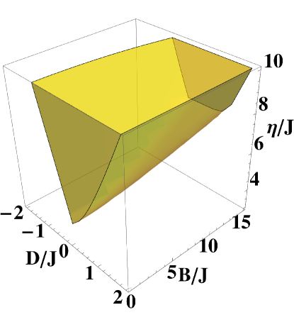
where is a diagonal matrix with elements the eigen-energy and is the particle-hole symmetric partner of . As we mentioned in the main text, for any , the positiveness of the diagonal elements determines the mean-field phase diagram of this quantum paramagnetic phase, and we show the diagram in Fig. S1 with parameters , as an example.
Figure S1: (Color online.) The quantum paramagnetic phase (shown as yellow region) with and .
It can also be checked that , and thus a proper Lagrangian should be
(S29)
Therefore, a bosonic vector potential and Berry curvature for can be defined as
(S30)
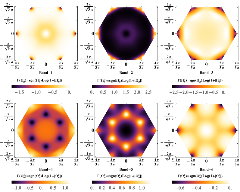
With the expression above, we show in Fig. S2 the Berry curvature distribution in the Brillouin zone. These finite values of Berry curvature lead to the non-zero bosonic band Chern numbers that we discussed in the main text. We also show the full diagram for all the six band Chern numbers in Fig. S3.
Figure S2: (Color online.) The distribution of Berry curvature (in log scale) in the momentum space from the lowest band (band-1) to the highest band (band-6) with a parameter choice as , , , and . Figure S3: Diagram of all six band Chern numbers distributions. The Chern numbers are listed from bottom to top. The parameters are the same as Fig. 3 in the main text. In addition to the band touching at and denoted by the red solid and black thick lines. There is band-touching at denoted by blue dashed lines that give rise to more complicated topological structures here.
III Collinear case
In this section, we derive Eq. (8) in the main text. We first take and into Eq. (S9)-(S11), and to further simplify the expression, we then perform a gauge transformation as and . The Hamiltonian matrix in the basis
is expressed as
(S43)
Now with the basis transformation that we mentioned in the main text: and , we can obtain with , where
(S44)
or alternatively,
(S45)
as written in Eq. (8) of the main text (up to a constant), where we have used the fact that and .
Since is Hermitian, we can diagonalize by a unitary matrix as with .
Then, it can be found that
(S46)
can diagonalize as
(S47)
while transforming the commutator into the canonical bosonic commutator with particle (hole) eigen-energy , and thus is the proper wavefunctions for the “phononic” Hamiltonian Eq. (S17). It can be noticed that fully depends on and does not change with non-zero . Therefore, we have the conclusion in the main text that the topological properties of Hamiltonian are fully determined by .