Persistence Norms and the Datasaurus

Abstract

Topological Data Analysis (TDA) provides a toolkit for the study of the shape of high dimensional and complex data. While operating on a space of persistence diagrams is cumbersome, persistence norms provide a simple real value measure of multivariate data which is seeing greater adoption within finance. A growing literature seeks links between persistence norma and teh summary statistics of the data being analysed. This short note targets the demonstration of differences in the persistence norms of the Datasaurus datasets of matejka2017same. We show that persistence norms can be used as additional measures that often discriminate datasets with the same collection of summary statistics. Treating each of the data sets as a point cloud we construct the $L_{1}$ and $L_{2}$ persistence norms in dimensions 0 and 1. We show multivariate distributions with identical covariance and correlation matrices can have considerably different persistence norms. Through the example, we remind users of persistence norms of the importance of checking the distribution of the point clouds from which the norms are constructed.

1 Introduction

Topological Data Analysis (TDA) concerns the study of the joint distribution of ordinal data. The TDA toolkit is equipped with many measures, such as the persistence norm, which allow the user to gain a summary of data shape. The datasaurus dozen of matejka2017same is presented as an important reminder that the mean, correlation and standard deviation of a bi-variate dataset do not provide sufficient information to understand the appearance of the scatter plot. In the language of TDA, the scatter plot of two variables may be thought of as a point cloud in which co-ordinates on the two axes define the locations of each point within the cloud. Through the calculation of the $L_{1}$ and $L_{2}$ persistence norms in dimensions 0 and 1 we demonstrate that the persistence norms do offer additional information about the point clouds. We show norms contain information over and above the means, variances and pairwise correlations of the constituent variables. Whilst the datasaurus dozen datasets satisfy the “same stats different graphs” requirement (matejka2017same), they have considerably different persistent norms.

Further value in the consideration of the datasaurus dozen lies in the ability to distinguish between datasets which offer higher $L_{1}$ and $L_{2}$ norms in dimension 1. $L_{1}$ and $L_{2}$ norms are often highly correlated in applications of TDA, rendering the consideration of cases where the two norms differ of additional importance. Where there are differentials in the two norms, further information is revealed from the dataset. $L_{1}$ norms are shown to reach a maximum when there are many smaller features in the dataset, whilst the highest $L_{2}$ norms occur when there are larger single features created by the points. Consequently, the datasaurus example acts to remind that although $L_{1}$ and $L_{2}$ norms are highly correlated, there is inference to be taken from any difference in their ratio. Where the choice is made to consider either $L_{1}$ or $L_{2}$ norms in empirical applications of TDA this note is a reminder that the decision is not made free of charge.

A final contribution from the calculation of the persistence norms of the datasaurus datasets is evidence that just looking at the $L_{1}$ and $L_{2}$ norms as additional measures on top of the standard summary statistics is still not sufficient to fully classify the different data sets. We show that many of the datasets have very similar norms. By adding the maximum distance between a pair of points in the dataset there is sufficient information to classify the data sets. However, with only 14 data sets considered in this paper it is only an exercise to demonstrate classification. In the practical implementation of persistence norms, far greater value is derived from the additional information embedded within the norms relative to correlations and variances, than is gained from metrics such as maximal separation between points. As the adoption of persistence norms accelerates, so it is important to understand how these norms relate to data shape.

Extending the discussion beyond the basic datasaurus datasets, we show the impact of a constant scaling being applied to all variables is simply to scale the persistence norms by the same constant. Translations, rotations or any other affine transformations of the point cloud do not alter the shape and therefore do not alter the persistence norms. When the cloud is scaled by different amounts on each axis the resultant distortion means the effect on the persistence norm is non-linear and different for each dataset. By plotting univariate distributions we learn more about the differences between the considered datasets, underlining the value in the metrics on the shape of multi-dimensional data provided by TDA. In all each extension the notion of the same first and second order moments is not violated, all differences in persistence norms continue to be understood through the differences in the shape of the point cloud.

This note contributes to a growing literature which seeks to understand how persistence norms relate to understood financial metrics. Following the early demonstration that persistence norms can act as an early warning signal for financial crashes (gidea2018topological; gidea2020topological) there has been a quest to understand why. aromi2021topological considers the role of the covariance matrix in determining norms and katz2022topological looks at the impact of noise on persistence norms. rudkin2023topology evidences that correlation and volatility alone do not explain persistence norms in cryptocurrency markets. rudkin2023uncertainty shows that there are links between persistence norms and uncertainty, but that there is still an unexplained component in the norms of financial markets. akingbade2023topological updates the discussion of gidea2018topological, linking crashes to periodicity. The question of how datasets with identical correlations and volatilities (standard deviations) can have different norms remains open. As we demonstrate in this note, distribution is a very important component of the link between norms and the summary statistics of data.

To accompany this note we provide a full R code which can be accessed through the website of Simon Rudkin. If using the code then please do not forget to cite this note and the R packages used therein.

2 Persistence Norms

The process of construction of persistence norms typically begins with a point cloud. In two dimensions the point cloud is simply the scatter plot. The co-ordinates of a point within the cloud are determined by the values of that point on each of the considered axes. The Datasaurus dozen are of interest because their respective point clouds all differ despite the fact that the means and standard deviations of the two variables that provide the axes, and correlations between the two axis variables, are identical. Herein we give an illustrative example for the construction of persistence norms. A fuller description of the mathematics underlying the diagrammatic illustration may be found in rudkin2023topology.

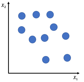
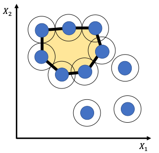
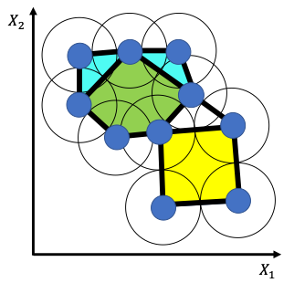
Figure 1: Construction of Dimension 1 Homology Classes

(a) Point cloud	(b) Filtration 1 ($\epsilon_{1}$)	(c) Filtration 2 ($\epsilon_{2}$)

Notes: Figures demonstrate the construction of persistence norms for an artificial data set with two variables, $X_{1}$ and $X_{2}$. Panel (a) is a scatter plot of the point cloud. A filtration of $\epsilon_{1}$ is applied in panel (b). To see the filtration circles of radius $\epsilon_{1}$ are drawn centred on each of the data points. Where the circles touch, or there is overlap, an edge is constructed between the points. A combination of edges is a dimension 0 feature. Where there exists an area enclosed by four or more points a shape is formed. In panel (a) the single shape is coloured orange. A shape formed within at least four points is a feature in dimension 1. Panel (c) applies a filtration of $\epsilon_{2}$. An edge is a dimension 0 feature. Where two dimension 0 features meet the longest lived feature remains and the shortest lived feature dies. A smaller shape is formed coloured green. Another shape is also born in the lower right coloured yellow.

Figure 1 demonstrates the process through which dimension 1 homology classes are formed. Through considering the dimension 1 homology classes the construction of the dimension 1 persistence norms is understood. In panel (a) the dataset is shown as a scatterplot with $X_{1}$ on the horizontal axis and $X_{2}$ on the vertical. In panel (b) a filtration of $\epsilon_{1}$ is applied and this is shown as a larger circle around each data point. Where those circles touch an edge is formed between the two data points. Edges are shown as thicker black lines. Where four or more points sit on the perimeter of a shape which does not have any edges crossing its interior, the resulting shape is a feature in dimension 1. In panel (b) there is a single dimension 1 feature. The birth of this feature is $\epsilon_{1}$ as there are many edges on the outside of the shape which are formed by the circles just touching. In panel (c) a larger filtration, $\epsilon_{2}$, is applied. Two edges now form across the corners of the original orange shape. These edges mean that the orange shape is no longer a dimension 1 feature and so that feature dies. New features are formed by the creation of the smaller green shape and a further feature in the lower right of the shape. These green and yellow coloured features in panel (c) thus have a birth filtration of $\epsilon_{2}$.

Dimension 0 features are based upon the connected components. Hence, they are merged by edges which form between the points. Firstly, zero dimensional features are supported in the data points themselves, this exists with a filtration 0. Subsequently, with an increasing filtration points are merged until only a single connected component is left. The obtained single connected component will always be there and so the first dimension 0 feature is infinitely lived. Whenever an edge forms a dimension 0 feature dies. Where two features join by an edge then we consider that the one which has the highest birth filtration dies and the feature with the earlier birth filtration, the longest-lived feature, continues. In Figure 1, Panel (a) we see 10 different connected components. Panel (b) shows four connected components, after seven initial ones are merged into one. In Panel (c) the final signle 0-dimensional feature is presented. Closer inspection will reveal that there are many balls which just touch in panel (b). For a filtration slightly below $\epsilon_{1}$ there will have been more dimension 0 features.

Given persistence diagrams in different dimensions, the norms for dimension $g$, $g\in\{0,1\}$ are computed using:

$$L_{g1}=\sum_{f=1}^{F_{g}}d_{f}-b_{f}$$ (1)

and:

$$L_{g2}=\sqrt{\sum_{f=1}^{F_{g}}(d_{f}-b_{f})^{2}}$$ (3)

Where in both cases, the second digit in the subscript informs that we are calculating the $L_{1}$ or $L_{2}$ norm. $F_{g}$ here denotes the number of features in dimension $g$. The lifetime for each feature, $f$, in dimension $g$ is computed using $d_{f}$ and $b_{f}$, being the birth, and death filtrations of feature $f$.

Within this note the persistence norms are constructed using the TDA package in R (TDAR2022). Full details of the technical implementation may be found in the documentation accompanying the package.

3 Data

Data used in this note is from matejka2017same and is included within the accompanying R package (datasauRus2022). Each dataset includes points described by two variables, $X_{1}$ and $X_{2}$ and is designed to have identical first and second moments. That is the average values of $X_{1}$ and $X_{2}$, $\mu_{1}$ and $\mu_{2}$ respectively, are identical. Likewise the standard deviations of both variables, $\sigma_{1}$ and $\sigma_{2}$ are also identical. The correlation between $X_{1}$ and $X_{2}$, $\rho_{12}$ is equal for every dataset. Specifically the datasets are created such that $\mu_{1}=54.27$, $\mu_{2}=47.84$, $\sigma_{1}=16.77$, $\sigma_{2}=26.94$ and $\rho_{12}=-0.064$. Table 1 provides summary statistics for the datasets to confirm the equality across all sets. For simplicity of exposition we refer to these datasets as having the same summary statistics.

Table 1: Datasaurus Data Summary Statistics

Dataset	Var	Mean	s.d.	Min	q25	q50	q75	Max
Dino	$X_{1}$	54.26	16.77	22.31	44.10	53.33	64.74	98.21
	$X_{2}$	47.83	26.94	2.95	25.29	46.03	68.53	99.49
Normal	$X_{1}$	54.26	16.77	9.18	42.42	57.43	66.91	100.05
	$X_{2}$	47.83	26.93	3.64	24.45	46.54	67.97	106.38
Away	$X_{1}$	54.27	16.77	15.56	39.72	53.34	69.15	91.64
	$X_{2}$	47.83	26.94	0.02	24.63	47.54	71.80	97.48
Bullseye	$X_{1}$	54.27	16.77	19.29	41.63	53.84	64.80	91.74
	$X_{2}$	47.83	26.94	9.69	26.24	47.38	72.53	85.88
Circle	$X_{1}$	54.27	16.76	21.86	43.38	54.02	64.97	85.66
	$X_{2}$	47.84	26.93	16.33	18.35	51.03	77.78	85.58
Dots	$X_{1}$	54.26	16.77	25.44	50.36	50.98	75.20	77.95
	$X_{2}$	47.84	26.93	15.77	17.11	51.30	82.88	94.25
H Lines	$X_{1}$	54.26	16.77	22.00	42.29	53.07	66.77	98.29
	$X_{2}$	47.83	26.94	10.46	30.48	50.47	70.35	90.46
High Lines	$X_{1}$	54.27	16.77	17.89	41.54	54.17	63.95	96.08
	$X_{2}$	47.84	26.94	14.91	22.92	32.50	75.94	87.15
Slant Down	$X_{1}$	54.27	16.77	18.11	42.89	53.14	64.47	95.59
	$X_{2}$	47.84	26.94	0.30	27.84	46.40	68.44	99.64
Slant Up	$X_{1}$	54.27	16.77	20.21	42.81	54.26	64.49	95.26
	$X_{2}$	47.83	26.94	5.65	24.76	45.29	70.86	99.58
Star	$X_{1}$	54.27	16.77	27.02	41.03	56.53	68.71	86.44
	$X_{2}$	47.84	26.93	14.37	20.37	50.11	63.55	92.21
V Lines	$X_{1}$	54.27	16.77	30.45	49.96	50.36	69.50	89.50
	$X_{2}$	47.84	26.94	2.73	22.75	47.11	65.85	99.69
Wide Lines	$X_{1}$	54.27	16.77	27.44	35.52	64.55	67.45	77.92
	$X_{2}$	47.83	26.94	0.22	24.35	46.28	67.57	99.28
X Shape	$X_{1}$	54.26	16.77	31.11	40.09	47.14	71.86	85.45
	$X_{2}$	47.84	26.93	4.58	23.47	39.88	73.61	97.84

Notes: Figures report the means, standard deviations, minimum, maximum and quartiles of the variables included within the Datasaurus datasets of matejka2017same. Dino is the original datasaurus, Normal is an additional dataset created for this paper which is comprised of two random normal variables with the same summary statistics and correlation as the datasaurus. The remaining 12 datasets are the datasaurus dozen of matejka2017same.

To those included in matejka2017same we add a further dataset in which both $X_{1}$ and $X_{2}$ are random draws from normal distributions. The Normal dataset has $X_{1}\sim N(\mu_{1},\sigma_{1}^{2})$ and $X_{2}\sim N(\mu_{2},\sigma_{2}^{2})$. As with the datasaurus dozen datasets, correlation between $X_{1}$ and $X_{2}$ is also -0.064. In many statistical applications we make the assumption of normally distributed variables and hence the Normal dataset is a useful example to present alongside the datasaurus dozen (matejka2017same). In total we have 14 datasets

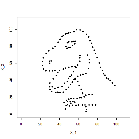
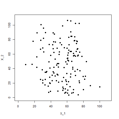
Figure 2: Scatter Plots

(a) Dino		(b) Normal
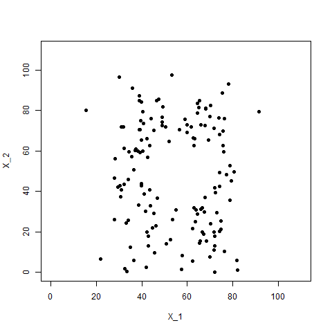
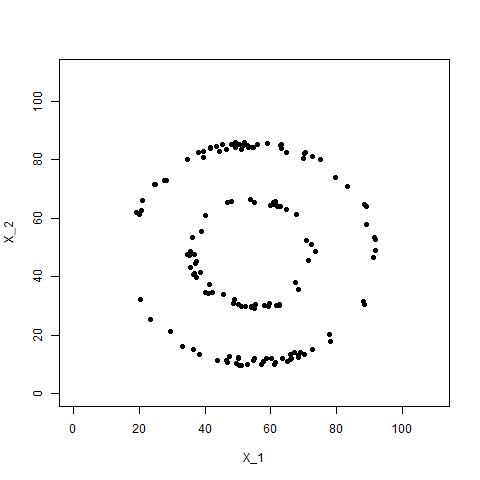
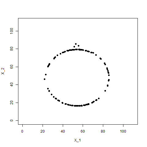
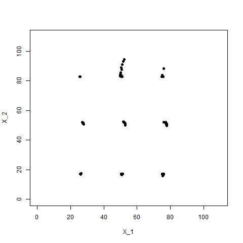
(c) Away	(d) Bullseye	(e) Circle	(f) Dots
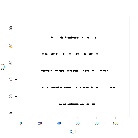
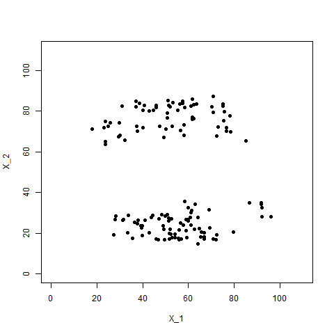
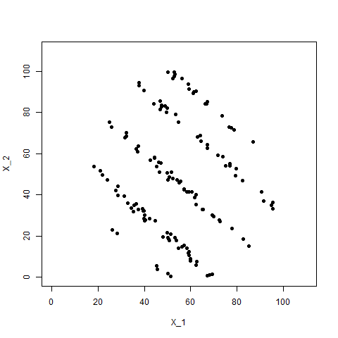
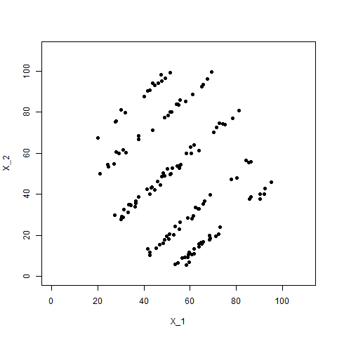
(g) H lines	(h) High lines	(i) Slant down	(j) Slant up
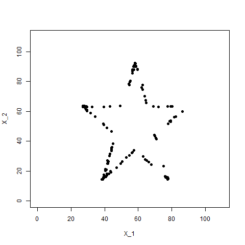
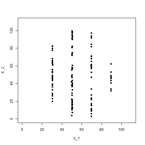
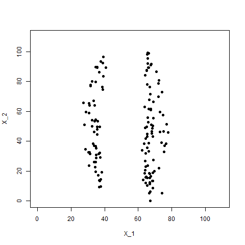
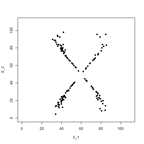
(k) Star	(l) V lines	(m) Wide lines	(n) X shape

Notes: Scatterplots of the original datasaurus dataset, the Normal cloud constructed in this paper and the datasaurus dozen of matejka2017same. All clouds are constructed from two variables, $X_{1}$ and $X_{2}$ with identical means, $\mu_{1}$, $\mu_{2}$, and standard deviations, $\sigma_{1}$, $\sigma_{2}$. For all datasets $\mu_{1}=54.27$, $\mu_{2}=47.84$, $\sigma_{1}=16.77$ and $\sigma_{2}=26.94$. Correlation between the two axis variables, $\rho_{12}$, is also identical in every panel. In all cases $\rho_{12}=-0.064$.