CA-PCA: Manifold Dimension Estimation, Adapted for Curvature

Abstract

The success of algorithms in the analysis of high-dimensional data is often attributed to the manifold hypothesis, which supposes that this data lie on or near a manifold of much lower dimension. It is often useful to determine or estimate the dimension of this manifold before performing dimension reduction, for instance. Existing methods for dimension estimation are calibrated using a flat unit ball. In this paper, we develop CA-PCA, a version of local PCA based instead on a calibration of a quadratic embedding, acknowledging the curvature of the underlying manifold. Numerous careful experiments show that this adaptation improves the estimator in a wide range of settings.

1 Introduction

Much of modern data analysis in high dimensions relies on the premise that data, while embedded in a high-dimensional space, lie on or near a submanifold of lower dimension. This allows one to embed the data in a space of lower dimension while preserving much of the essential structure, with benefits including faster computation and data visualization.

This lower dimension, hereafter referred to as the intrinsic dimension (ID) of the underlying manifold, often enters as a parameter of the dimension-reduction scheme. For instance, in each of the Johnson-Lindenstrauss-type results for manifolds by [13] and [4] the target dimension depends on the ID. Furthermore, the ID is a parameter of popular dimension reduction methods such as t-SNE [28] and multidimensional scaling [12, 16]. Therefore, it may be beneficial to estimate the ID before running further analysis since compressing the data too much may destroy underlying structure and it may be computationally expensive to re-run algorithms with a new dimension parameter, if such an error is even detectable. [6] uses their ID estimator to obtain sample complexity bounds for Generative Adversarial Networks (GANs). An interesting direct use of ID is found in [25], in which it is interpreted as a measure of complexity or variability for basketball plays. To similar effect, [3] uses intrinsic dimension to measure the complexity of the space of observed neural patterns in the human brain.

The literature on ID estimators is vast, and we refer the reader to [8] and [9] for a comprehensive review. We highlight recent progress of [14], as well as [18], [6], and [22], which prove results about the number of samples needed to estimate the ID with a given probability.

For our current analysis, we focus on the use of principle components analysis (PCA) as an ID estimator. There are a variety of ways this has been done (see [7, 17, 19, 24, 29]), but each version of local PCA works roughly by finding the eigenvalues of the covariance matrix for a data point and its nearest neighbors. The ID is then estimated using the fact that we expect the eigenvalues to be high for eigenvectors which are close to the tangent space of the underlying manifold and the eigenvalues to be low for eigenvectors which are nearly orthogonal to the tangent space. We expect $d$ eigenvalues to be larger than the rest, where $d$ is the ID. The remaining $D-d$ eigenvalues will be small, but often nonzero due to effects of curvature or error in measurement.

Local PCA and other ID estimators are often calibrated via a subspace or unit ball intersected with a subspace. While a manifold may be locally well-approximated by its tangent space near a point, in practice one may not always have enough sampled data to zoom in sufficiently close. Our key insight is that if one expects data to lie on a manifold with nontrivial curvature rather than a subspace, we should calibrate the ID estimator using a manifold with nontrivial curvature rather than a subspace. In particular, our main contribution is to calibrate a version of local PCA to a quadratic embedding, producing a new ID estimator, which we deem curvature-adjusted PCA (CA-PCA). Provided the underlying manifold is $C^{2}$-smooth, it will be well-approximated by a quadratic embedding, in fact, better approximated than by its tangent plane.

In principle, this insight could be applied to any number of existing ID estimators. We choose to apply it to a single estimator for which the adjustment is relatively simple, then test the new version extensively. In particular, we adapt a version of local PCA found in [22] for the curvature of a manifold and apply the new version to various examples of data sampled from manifolds. We note that this adaption of local PCA necessitates an entirely novel analysis.

The main benefit of our estimator is that we are better able to estimate the ID in cases where the sample size is small. It allows one to consider either a larger number of nearest neighbors for the ID estimation as it adjusts for the neighborhood starting to “go around” the manifold or a smaller number of nearest neighbors with the increased power to distinguish between whether the variance in eigenvalues is due to curvature or statistical noise. Our method achieves this increase in accuracy by regularizing fit of the eigenvectors of the data to a curvature adjusted benchmark.

The use of quadratic embeddings for data lying on or near a manifold is not new. It was used to approximate a manifold (of known dimension) in [1] and [11]. [21] approximate manifolds with spherelets. [27] consider the application of PCA to neighborhoods of a manifold modeled via quadratic embedding to analyze estimation of tangent space, yet does not consider ID estimation. However, to the best of our knowledge, this is the first time quadratic embeddings have been used in combination with PCA to estimate the ID of a manifold.

Our paper is outlined as follows. In Section 2, we describe the version of local PCA found in [22]. In Section 3, we compute the limiting distribution of eigenvalues expected for the covariance matrix of a quadratic embedding, which is then used to derive our test. The formal calculations are saved for Appendix A. Experiments on data sampled from manifolds, both synthetic and simulated, are described in Section 4. Discussion is in Section 5.

2 Background and Problem Setup

Let $\{x_{1},...,x_{k}\}$ be a sample of points in $\mathbb{R}^{D}$. The covariance matrix $\Sigma[x_{1},...,x_{k}]$ of this sample is constructed as follows. Let $\bar{x}=\frac{1}{k}\sum_{i=1}^{k}x_{i}$ and define

$$\hat{\Sigma}[x_{1},...,x_{k}]=\frac{1}{k-1}\sum_{i=1}^{k}(x_{i}-\bar{x})(x_{i}-\bar{x})^{T},$$

where $\bar{x}$ and each $x_{i}$ are interpreted as column vectors. A continuous version $\Sigma[\mu]$ may be computed for finite measures $\mu$ on $\mathbb{R}^{D}$ by replacing the summation with integration and dividing by the total volume of $\mu$. Observe that $\hat{\Sigma}[x_{1},...,x_{k}]$ and $\Sigma[\mu]$ are always symmetric, positive semidefinite matrices. Let $\vec{\lambda}\hat{\Sigma}[x_{1},...,x_{k}]$ denote a vector consisting of the eigenvalues of $\hat{\Sigma}[x_{1},...,x_{k}]$ in decreasing order and similarly for $\vec{\lambda}\Sigma[\mu]$.

The idea behind using local PCA for ID estimation is that if $x_{1},...,x_{k}$ are sampled from a small neighborhood where the underlying manifold is well-approximated by its $d$-dimensional tangent space, then one expects the first $d$ elements of $\vec{\lambda}\hat{\Sigma}[x_{1},...,x_{k}]$ to be much larger than the last $D-d$ elements. There are many ways to translate this observation into practice; see citations in the Introduction for reference. Here, we focus on a formulation of the test described by [22] which requires no human judgment or arbitrary threshold cutoffs; presents the possibility of a simple modification to adjust for curvature of the underlying manifold; and is supported by evidence from our experiments as well as proof of statistical convergence [22].

Lemma 2.1 ([22]).

Let $W$ be a $d$-dimensional subspace of $\mathbb{R}^{D}$ ($D\geq d$) and let $\nu$ denote the $d$-dimensional Lebesgue measure on $W$ intersected with the unit ball of $\mathbb{R}^{D}$. Then

$$\vec{\lambda}\Sigma[\nu]:=\vec{\lambda}(d,D):=\frac{1}{d+2}(\underset{d\text{ times}}{\underbrace{1,...,1}},\underset{D-d\text{ times}}{\underbrace{0,...,0}}).$$

An elementary argument shows that for $r>0$ and $v\in\mathbb{R}^{D}$,

$$\frac{1}{r^{2}}\vec{\lambda}\hat{\Sigma}[rx_{1}-v,...,rx_{k}-v]=\vec{\lambda}\hat{\Sigma}[x_{1},...,x_{k}].$$

Thus, given points sampled from a $d$-dimensional ball of radius $r$ centered away from the origin in $\mathbb{R}^{D}$, we expect $1/r^{2}$ times the associated eigenvalues to be close to $\vec{\lambda}(d,D)$.

Let $X\subset\mathbb{R}^{D}$ be a collection of points, presumably on or near a $d$-dimensional manifold embedded in $\mathbb{R}^{D}$. Let $x\in X$ and $\{x_{1},...,x_{k}\}$ be the neighbors of $x$ in $X$ lying within distance $r$ of $x$. Then, the test described in [22] determines an estimated ID $\hat{d}$ at $x$ by

$$\hat{d}=\operatorname*{argmin}_{d}\left\|\frac{1}{r^{2}}\vec{\lambda}\hat{\Sigma}[x_{1},...,x_{k}]-\vec{\lambda}(d,D)\right\|_{2}.$$

3 Theoretical Analysis to set the stage for CA-PCA

Before we specify the CA-PCA algorithm, we establish several theoretical results that help us set the stage for the algorithm. We delineate the limiting distribution of the eigenvalues of the covariance matrix for the uniform distribution on a Riemannian manifold of dimension $d$.

3.1 Limiting Distribution of Eigenvalues

Given a $C^{2}$, $d$-dimensional manifold $\mathcal{M}\subset\mathbb{R}^{D}$ and a point $p\in\mathcal{M}$, there exists an orthonormal set of coordinates $(x_{1},...,x_{D})$ for $\mathbb{R}^{D}$ such that $\mathcal{M}$ is locally the graph of a $C^{2}$ function $F:\mathbb{R}^{d}\to\mathbb{R}^{D-d}$. Without loss of generality, we take $p$ to be the origin in $\mathbb{R}^{D}$.

Since $F$ is well-approximated by its Taylor series of order 2, we consider the quadratic embedding

$$Q:(x_{1},...,x_{d})\mapsto(x_{1},...,x_{d},Q_{1}(x_{1},...,x_{d}),...,Q_{D-d}(x_{1},...,x_{d})),$$ (1)

where $Q_{j}:\mathbb{R}^{d}\to\mathbb{R}$ is a quadratic form of the form $Q_{j}(x)=x^{T}M_{j}x$ for a symmetric $d\times d$ matrix $M_{j}$ ($1\leq j\leq D-d$). We denote the eigenvalues of $M_{j}$ as $\lambda_{j,1},...,\lambda_{j,d}$. Denote the graph of $Q$ as $\mathcal{M}_{Q}$ and the $d$-dimensional Riemannian volume form on $\mathcal{M}_{Q}$ by $d\mu_{Q}$.

Our goal is to compute the eigenvalues of the covariance matrix for the uniform (with respect to $\mu_{Q}$) distribution on $\mathcal{M}_{Q}\cap B_{r}(0)$ for some radius $r>0$. By rescaling, take $r=1$. We denote this matrix $\Sigma$. For this purpose, we define $S:\mathbb{R}^{d}\to\mathbb{R}$, the density function with respect to $d\mu_{Q}$, as $d\mu_{Q}(x_{1},...,x_{d})=S(x_{1},...,x_{d})dx$, where $dx$ is the Lebesgue measure on $\mathbb{R}^{d}$.

Define quadratic forms $\tilde{Q}_{j}(x)=x^{T}M_{j}^{2}x$, and note that the eigenvalues of the matrix $M_{j}^{2}$ are $\lambda_{j,1}^{2},...,\lambda_{j,d}^{2}$. Let $\Lambda=\max_{1\leq k\leq D-d}\|M_{k}\|$.

Lemma 3.1.

Under the above assumptions and notation, the density function of $d\mu_{Q}$ is

$$S(x)=1+2\sum_{j=1}^{D-d}\tilde{Q}_{j}(x)+O(\Lambda^{4}).$$ (2)

Proof.

Given (1),

$$S(x)=\sqrt{|\det(g_{ij}(x))_{1\leq i,j\leq d}|},$$

where $g_{ij}(x)=g_{i}(x)\cdot g_{j}(x)$ and

$$g_{i}(x)=\left(0,...,1,...,0,\frac{\partial Q_{1}}{\partial x_{i}}(x),...,\frac{\partial Q_{D-d}}{\partial x_{i}}(x)\right).$$

Since $\nabla Q_{j}(x)=2M_{j}x$, we have

$$g_{i}(x)=\left(0,...,1,...,0,(2M_{1}e_{i})\cdot x,...,(2M_{D-d}e_{i})\cdot x\right),$$

where $e_{1},...,e_{d}$ is the standard ordered basis of $\mathbb{R}^{d}$.

Thus,

$$g_{ij}(x)=\delta_{ij}+\sum_{k=1}^{D-d}(2M_{k}e_{i}\cdot x)(2M_{k}e_{j}\cdot x),$$ (3)

and the trace of the matrix $(g_{ij})=(g_{ij})_{1\leq i,j,\leq d}$ is

$$\text{Tr}(g_{ij}(x))=d+\sum_{j=1}^{D-d}\sum_{i=1}^{d}\left|2M_{j}e_{i}\cdot x\right|^{2}.$$ (4)

Consider a symmetric $d\times d$ matrix $M$ with columns $m_{1},...,m_{d}$ (thus $Me_{i}=m_{i}$). Then,

$$x^{T}M^{2}x=(x^{T}M^{T})\cdot(Mx)=\|Mx\|^{2}=\sum_{i=1}^{d}|m_{i}\cdot x|^{2}.$$ (5)

Plugging (5) applied to $M=M_{j}$ ($1\leq j\leq D-d$) into (4),

$$\text{Tr}(g_{ij}(x))_{1\leq i,j\leq d}=d+4\sum_{j=1}^{D-d}\tilde{Q}_{j}(x).$$ (6)

By (3), the difference of $(g_{ij}(x))_{1\leq i,j\leq d}$ and the identity matrix has entries of order $O(\Lambda^{2})$. Thus, the eigenvalues of $(g_{ij}(x))_{1\leq i,j\leq d}$ each differ from 1 by $O(\Lambda^{2})$. That is, for fixed $x_{0}$, and denoting the eigenvalues of $(g_{ij}(x_{0}))_{1\leq i,j\leq d}$ by $\mu_{1},...,\mu_{d}$,

$$\mu_{i}=1+c_{i},$$

where $c_{i}=O(\Lambda^{2})$ and

$$\sum_{i}c_{i}=4\sum_{j=1}^{D-d}\tilde{Q}_{j}(x_{0}).$$

Thus,

$$\det(g_{ij}(x))=\prod_{i=1}^{d}(1+c_{i})=1+4\sum_{j=1}^{D-d}\tilde{Q}_{j}(x)+O(\Lambda^{4}).$$

By the Taylor expansion $\sqrt{1+t}=1+\frac{1}{2}t+O(t^{2})$, we have the desired conclusion. ∎

Recall, our goal is to compute the eigenvalues of the covariance matrix $\Sigma$. Let

$$R=\{x\in\mathbb{R}^{d}:|x|^{2}+\sum_{j=1}^{D-d}(Q_{j}(x))^{2}\leq 1\}$$

and

$$\tilde{S}(x)=\frac{S(x)}{\int_{R}S(x)dx}.$$

Then, each of the entries of $\Sigma$ is of one of the following forms

1. $I_{1}(i)=\int_{R}(x_{i}-\bar{x}_{i})^{2}\tilde{S}(x)dx$ ($1\leq i\leq d$)

2. $I_{2}(i,j)=\int_{R}(x_{i}-\bar{x}_{i})(x_{j}-\bar{x}_{j})\tilde{S}(x)dx$ ($1\leq i\neq j\leq d$)

3. $I_{3}(i,j)=\int_{R}(x_{i}-\bar{x}_{i})(Q_{j}(x)-\bar{Q}_{j})\tilde{S}(x)dx$ ($1\leq i\leq d,1\leq j\leq D-d$)

4. $I_{4}(i)=\int_{R}(Q_{i}(x)^{2}-\bar{Q}_{i}^{2})\tilde{S}(x)dx$ ($1\leq i\leq D-d$)

5. $I_{5}(i,j)=\int_{R}(Q_{i}(x)-\bar{Q}_{i})(Q_{j}(x)-\bar{Q}_{j})\tilde{S}(x)dx$ ($1\leq i\neq j\leq D-d$),

where

$$\bar{x}_{i}=\int_{R}x_{i}\tilde{S}(x)dx,\hskip 18.06749pt\bar{Q}_{i}=\int_{R}Q_{i}(x)\tilde{S}(x)dx.$$

Since $x_{i}$ is an odd function and $R$ is a region symmetric about the origin, we immediately see that $\bar{x}_{i}=0$ for $1\leq i\leq d$. Furthermore, $Q_{j}(x)-\bar{Q}_{j}$ is an even function and $x_{i}-\bar{x}_{i}=x_{i}$ is odd, so $I_{3}(i,j)=0$ for all $1\leq i\leq d,1\leq j\leq D-d$. As a result, $\Sigma$ is a block diagonal matrix with an upper block $\Sigma_{1}$ of size $d\times d$ and a lower block $\Sigma_{2}$ of size $(D-d)\times(D-d)$, that is

$$\Sigma=\left[\begin{array}[]{c|ccc}\Sigma_{1}&&0&\\ \hline\cr&&&\\ 0&&\Sigma_{2}&\\ &&&\end{array}\right].$$ (7)

In [27], the authors consider separately the “uncorrelated case,” corresponding to taking $I_{5}(i,j)=0$ for all $1\leq i\neq j\leq D-d$ above. One could use this assumption to calculate the eigenvalues of $\Sigma_{2}$ explicitly ($\frac{2}{(d+2)^{2}}A_{j}$, as will be shown in the proof of Proposition 3.2); however, only the sum of these eigenvalues will be needed for comparison with the eigenvalues of $\Sigma_{1}$, so we avoid making this assumption ourselves.

This motivates the statement of our main proposition. To simplify the following expressions, we fix the notation

$$A_{j}=\sum_{k=1}^{d}\lambda_{j,k}^{2},\hskip 7.22743ptA=\sum_{j=1}^{D-d}A_{j}=\sum_{j,k}\lambda_{j,k}^{2}$$

and

$$B_{j}=\left(\sum_{k=1}^{d}\lambda_{j,k}\right)^{2},\hskip 7.22743ptB=\sum_{j=1}^{D-d}B_{j}=\sum_{j}\left(\sum_{k}\lambda_{j,k}\right)^{2}.$$

Observe that each of $A,A_{j},B,B_{j}$ is $O(\Lambda^{2})$.

Proposition 3.2.

Let $\Sigma_{1},\Sigma_{2}$ be as above. Denote the eigenvalues of $\Sigma_{1}$ by $\lambda_{1},...,\lambda_{d}$. Then $\text{Tr}(\Sigma_{1})$ is

$$\frac{d}{d+2}+\frac{4d-2d^{2}}{(d+2)^{3}(d+4)}A-\frac{3d+4}{(d+2)^{2}(d+4)}B+O(\Lambda^{4})$$ (8)

and $\text{Tr}(\Sigma_{2})$ is

$$\frac{2}{(d+2)^{2}}A+O(\Lambda^{3}).$$ (9)

Furthermore, for $1\leq i\leq d$, $\lambda_{i}$ lies between

$$\frac{1}{d+2}-\frac{20d^{2}+82d+76}{(d+2)^{3}(d+4)}A-\frac{11d+24}{2(d+2)^{2}(d+4)}B$$ (10)

and

$$\frac{1}{d+2}+\frac{5d^{2}+18d+24}{(d+2)^{3}(d+4)}A+\frac{d}{2(d+2)^{2}(d+4)}B$$ (11)

up to an error of $O(\Lambda^{4})$.

The bounds in (10) and (11) are not sharp. Our method of proof ignores much potential cancellation; however, it still reveals that $|\frac{1}{d+2}-\lambda_{i}|\leq O(d^{-2}\sum_{j=d+1}^{D}\lambda_{j}^{2})$.

In order to determine $\text{Tr}(\Sigma_{1})$ and $\text{Tr}(\Sigma_{2})$, we only need the diagonal entries of $\Sigma$, that is, the integrals $I_{1}(i)$ and $I_{4}(j)$. To determine the bounds on $\lambda_{1},...,\lambda_{d}$, we compute $I_{1}(i)$ with $x_{i}$ replaced by an arbitrary direction which may be chosen to maximize or minimize the integral. We perform these computations in Appendix A. The method is long, but a straightforward application of integration in radial coordinates, integration of polynomial functions over the sphere, truncation of Taylor series, and Lemma 3.1.

Since $B$ may not generally be calculated as a function of $A$, we have not yet achieved an explicit relation between $\text{Tr}(\Sigma_{1})$ and $\text{Tr}(\Sigma_{2})$. We take our “best guess” of how they may relate to be the expectation of what occurs when the eigenvalues are of random sign. Specifically, let $\epsilon_{1,j},...,\epsilon_{d,j}$ be i.i.d. variables taking on value 1 and -1, each with probability 1/2. Let $\lambda_{i,j}=\epsilon_{i,j}\alpha_{i,j}$, where $\alpha_{i,1},...,\alpha_{i,d}$ are fixed. Then,

$$\mathbb{E}B_{j}=\mathbb{E}(\sum_{i=1}^{d}\epsilon_{i,j}\lambda_{i,j})^{2}=\mathbb{E}\sum_{1\leq i_{1},i_{2}\leq d}\epsilon_{i_{1},j}\epsilon_{i_{2},j}\lambda_{i_{1},j}\lambda_{i_{2},j}=\sum_{i=1}^{d}\lambda_{i,j}^{2}=A_{j}.$$

Thus, for the purpose of deriving our test in Subsection 3.2 we will assume $A_{j}=B_{j}$ for all $1\leq j\leq D-d$. In particular, $A=B$. Since in practice $D-d$ is often large, it may be reasonable to use expectation as above.

Substituting $A=B$ into (8),

$$\text{Tr}(\Sigma_{1})=\frac{d}{d+2}-\frac{5d^{2}+6d+8}{(d+2)^{3}(d+4)}A$$ (12)

with average eigenvalue

$$\frac{1}{d+2}-\frac{5d^{2}+6d+8}{d(d+2)^{3}(d+4)}A.$$ (13)

3.2 CA-PCA Algorithm

Algorithm 1 CA-PCA

  Input: $X,N,k$

  for $n=1,...,N$ do

     Sample $x\in X$ uniformly at random

     Choose $\{x_{1},...,x_{k+1}\}$ $(k+1)$-nearest neighbors to $x$

     Set $r=(\|x-x_{k}\|_{2}+\|x-x_{k+1}\|_{2})/2$

     Form $\hat{\Sigma}[x_{1},...,x_{k}]$

     Calculate eigenvalues

$$(\hat{\lambda}_{1},...,\hat{\lambda}_{D})=\frac{1}{r^{2}}\vec{\lambda}\hat{\Sigma}[x_{1},...,x_{k}]$$

     for $d=1,...,D$ do

        Compute $(\lambda^{(d)}_{1},...,\lambda^{(d)}_{D})$ by substituting $\hat{\lambda}_{1},...,\hat{\lambda}_{D}$ into (14)

     end for

     Solve

$$\hat{d}^{(n)} =\operatorname*{argmin}_{1\leq d\leq D}\|\vec{\lambda}(d,D)-(\lambda^{(d)}_{1},...,\lambda^{(d)}_{D})\|_{2}$$

$$+\frac{1-\delta_{D}(d)}{D-d}\|(\hat{\lambda}_{1},...,\hat{\lambda}_{D})-(\lambda^{(d)}_{1},...,\lambda^{(d)}_{D})\|_{1}$$

  end for

  Return Mean $(\hat{d}^{(1)},...,\hat{d}^{(N)})$

Proposition 3.2 provides a formula for $\sum_{i=1}^{d}\lambda_{i}=\text{Tr}(\Sigma_{1})$. Ideally, we would like to know the individual values of $\lambda_{i}$ to compare to the eigenvalues coming from the sampled points. However, in practice, we are only given the sampled eigenvalues so we will assume that each $\lambda_{i}$ is equal. This is a reasonable assumption given the bounds in (10) and (11). Furthermore, the sampled eigenvalues may differ from each other due to statistical noise, so it may be faulty to assume the difference is due to curvature effects in $\mathcal{M}$.

Thus, we assume

$$\lambda_{i}=\frac{1}{d+2}-c_{h}(d)A,1\leq i\leq d,$$

where $c_{h}(d)=\frac{5d^{2}+6d+8}{d(d+2)^{3}(d+4)}$ by (13). We assume $\Lambda$ is small so we may ignore the $O(\Lambda^{4})$ terms.

Letting $c_{l}(d)=\frac{1}{(d+2)^{2}}$, rewrite (9) as

$$\sum_{j=d+1}^{D}\lambda_{j}=c_{l}(d)\sum_{j=1}^{D-d}A_{j-d}=c_{l}(d)A.$$

By substitution,

$$\frac{1}{d+2}=\lambda_{i}+\frac{c_{h}(d)}{c_{l}(d)}\sum_{j=d+1}^{D}\lambda_{j}=\lambda_{i}+c(d)\sum_{j=d+1}^{D}\lambda_{j}.$$

by setting $c(d)=c_{h}(d)/c_{l}(d)=(5d^{2}+6d+8)/(d(d+2)(d+4))$.

Given $x\in X$, let $x_{1},...,x_{k+1}$ denote the $k+1$ nearest neighbors of $x$, in increasing order of distance from $x$. Let $r=(\|x-x_{k}\|_{2}+\|x-x_{k+1}\|_{2})/2$ and determine sample eigenvalues $\hat{\lambda}_{1}\geq...\geq\hat{\lambda}_{D}$ from the matrix $\frac{1}{r^{2}}\hat{\Sigma}[x_{1},...,x_{k}]$. Under our small $\Lambda$ assumption we expect that as the number of samples increases, $(\hat{\lambda}_{1},...,\hat{\lambda}_{d})$ will converge to the eigenvalues of $\Sigma_{1}$ and $(\hat{\lambda}_{d+1},...,\hat{\lambda}_{D})$ will converge to the eigenvalues of $\Sigma_{2}$. Thus, we will treat $(\hat{\lambda}_{1},...,\hat{\lambda}_{d})$ as “coming from” $\Sigma_{1}$ and expect

$$\lambda^{(d)}_{i}:=\hat{\lambda}_{i}+c(d)\sum_{j=d+1}^{D}\hat{\lambda}_{j}\approx\frac{1}{d+2},1\leq i\leq d.$$ (14)

Setting $\lambda^{(d)}_{j}=0$ for $d+1\leq j\leq D$, we are tempted to choose $1\leq d\leq D$ to minimize the quantity

$$\|\vec{\lambda}(d,D)-(\lambda^{(d)}_{1},...,\lambda^{(d)}_{D})\|_{2}=\sqrt{\sum_{i=1}^{d}\Big{(}\frac{1}{d+2}-\lambda^{(d)}_{i}\Big{)}^{2}}.$$ (15)

However, a small amount of statistical noise can easily lead us to pick the wrong value of $d$.

For example, suppose our data are sampled from $\mathbb{R}^{2}$ and determine the eigenvalues $(0.21,0.15)$. Taking $d=2$, the value of (15) is $\|(0.25,0.25)-(0.21,0.15)\|_{2}=.1077$. Taking $d=1$, then we add $19/15*0.15$ back to $0.21$ to get $(\lambda^{(1)}_{1},\lambda^{(1)}_{2})=(0.4,0)$, then compute (15) to be $\|(1/3,0)-(.4,0)\|_{2}=0.0667$. We pick the dimension corresponding to the smaller error; thus, $d=1$.

However, the second eigenvalue 0.15 in this example corresponds to a very high curvature of our manifold. For the quadratic embedding $x\mapsto(x,cx^{2})$, our model predicts $c=\sqrt{27/40}$, in which case we are working at larger scales relative to our manifold, violating small $\Lambda$ assumptions.

Thus, we choose $1\leq d\leq D$ to minimize

$$\|\vec{\lambda}(d,D)-(\lambda^{(d)}_{1},...,\lambda^{(d)}_{D})\|_{2}+\frac{1-\delta_{D}(d)}{D-d}\|(\hat{\lambda}_{1},...,\hat{\lambda}_{D})-(\lambda^{(d)}_{1},...,\lambda^{(d)}_{D})\|_{1},$$ (16)

where $\delta_{D}(D)=1$ and $\delta_{D}(d)=0$ for $d\neq D$. (In the case $d=D$, we take 0/0=0.)

Here, the second term in (16) is taken to represent an implied notion of the curvature of the manifold. We use the $\ell^{1}$ norm since the lower eigenvalues have an additive effect in modifying the upper ones. Furthermore, a $1/(D-d)$ weight is chosen for this second term to make it represent the average of the lowest $D-d$ eigenvalues, or in other words, the average of the curvatures of all of the $Q_{j}$. If our data were to be remeasured with an additional feature/dimension, we would need to include an additional $Q_{j}$ to describe the embedding; however, this shouldn’t change the ID nor the eigenvalues of the other $Q_{j}$.

One may consider this modification as analogous to LASSO, in which one attempts to minimize an $\ell^{2}$ error in conjunction with the size of the coefficients.

4 Experiments

4.1 Outline

We ran CA-PCA on a number of examples of point clouds, each contained in $\mathbb{R}^{D}$ for some $D$ and (presumably) sampled from manifolds. The results were compared with the approach from [22] (PCA) and the maximum likelihood estimator from [20] (LB).

To fully compare CA-PCA to all other existing, competitive ID estimators would be onerous. [8] provides five criteria for a successful estimator: computaional feasability, robustness to multiscaling, robustness to high dimension, a work envelope, and accuracy. Among eleven estimators, none is the clear favorite as different tests satisfy different criteria. For this reason, and to reflect our main insight, we emphasize a comparison between CA-PCA and PCA. However, we still compare CA-PCA with LB to demonstrate that our estimator is at least competitive with another popular version.

Given a point cloud $X\subset\mathbb{R}^{D}$, a random point of $X$ was sampled, denoted $x$. The $k$ nearest neighbors of $x$ were computed and used to run principle components analysis, from which $D$ eigenvalues were obtained. These eigenvalues were normalized by multiplying by $1/r^{2}$, where $r$ was chosen by taking the arithmetic mean of the distance of the $k$-th nearest neighbor of $x$ and the distance of the $(k+1)$-st nearest neighbor of $x$. The CA-PCA test was run to determine an estimated ID. This process was repeated by sampling $N$ points randomly with replacement from $X$ and all of the estimated dimensions were averaged to produce a final estimate. An average estimated ID was then computed over a range of values of $k$, although the same points $x$ were sampled for each $k$ to reduce time spent computing the nearest neighbors. Our results are depicted by graphing the averaged estimated ID as a function of $k$ and comparing to the actual ID $d$. $N=200$ unless otherwise stated.

The same process was used for the PCA and LB tests, except for the LB test no computation or rescaling of eigenvalues was needed, merely distances between points. Also, the same randomly sampled points $x$ were used for each test.

In the case of point clouds in $\mathbb{R}^{D}$ for large $D$ (see Isomap faces and airplane photos below), the $D-k$ tail eigenvalues equal to zero were removed, in effect replacing the normalizing factor $\frac{1}{D-d}$ by $\frac{1}{k-d}$.

When possible, manifolds are chosen to be without boundary, as points sampled from boundaries may produce a consistent underestimation of the ID, introducing a bias which may interfere with simple comparison of PCA and CA-PCA.

4.2 Some Synthetic Data

One possible parametrization for a Klein bottle embedded in $\mathbb{R}^{4}$ is given by

$$x =(a+b\cos(v))\cos(u)$$

$$y =(a+b\cos(v))\sin(u)$$

$$z =b\sin(v)\cos(u/2)$$

$$w =b\sin(v)\sin(u/2)$$

for $u,v\in[0,2\pi)$. Choosing $a=10$ and $b=5$, 400 points were sampled via the uniform distribution for $u,v$ on $[0,2\pi)^{2}$.

Running the three tests on these 400 points, we see that both PCA and CA-PCA appear to converge to the correct dimension of 2, although the latter is much faster (see Figure 1(a)). The LB estimator fails to converge, though it is much closer to 2 than 3. On this note, it is also clear that CA-PCA provides an estimated dimension closer to 2 than 1 for smaller values of $k$ than PCA.

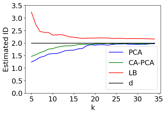
(a) Estimated ID for Klein bottle in $\mathbb{R}^{4}$

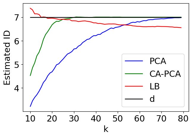
(b) Estimated ID for $S^{7}\subset\mathbb{R}^{8}$

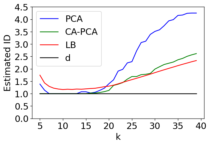
(c) Estimated ID for curve in $\mathbb{R}^{8}$

Figure 1: Results for Synthetic Data

We randomly sampled 5,000 points from the unit sphere $S^{7}\subset\mathbb{R}^{8}$ with respect to the uniform measure. Here, CA-PCA converges to the true dimension of 7 much faster than PCA (see Figure 1(b)). While LB reaches the true dimension first, the estimate decreases (gets worse) as $k$ increases.

For $S^{7}$ and the Klein bottle, CA-PCA consistently produces a higher estimated ID than PCA. One may suspect that this behavior partially explains some of the faster convergence; however, the next example shows that CA-PCA can produce a lower estimate than PCA.

Consider the parametrization of a curve in $\mathbb{R}^{8}$ via the map

$$\theta\mapsto(\cos\theta,\sin\theta,\cos 2\theta,...,\cos 4\theta,\sin 4\theta),\theta\in[0,2\pi).$$

A point cloud in $\mathbb{R}^{8}$ was determined by sampling 100 points from this curve, uniformly randomly over $\theta\in[0,2\pi)$. The results of the tests are shown in Figure 1(c). As the number of nearest neighbors increases and the collection of nearest neighbors wraps further around the curve, each of the tests provides an estimated ID increasingly higher than the true ID of 1. However, CA-PCA does so at a slower rate than PCA and provides a lower ID than PCA for each value of $k$.

We next move to some more difficult examples, where both the dimension and codimension are higher than in most previous examples. In Figure 2(a), we have the results of the tests applied to 20,000 points sampled randomly from $SO(5)$ with respect to the Haar measure and viewed as 5x5 matrices (thus as elements of $\mathbb{R}^{5\times 5}\cong\mathbb{R}^{25}$). Here, CA-PCA overshoots the dimensions for larger values of $k$ and becomes a worse predictor than PCA. However, it still gets closer to the true dimension of 10 for low values of $k$ and stays within a reasonable range.

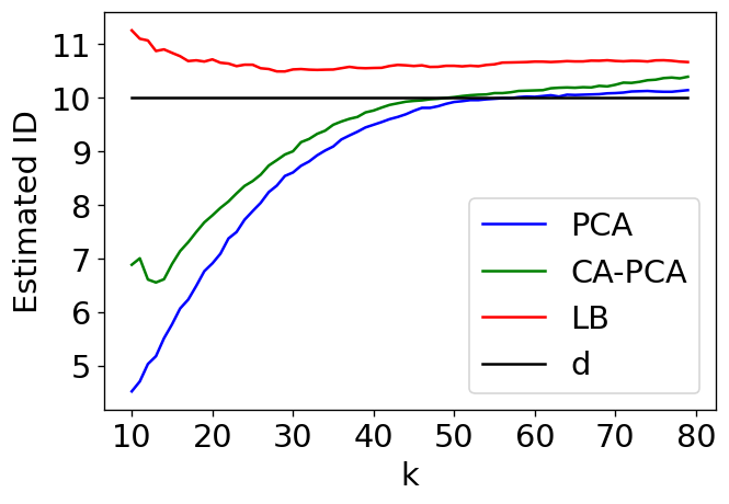
(a) Estimated ID for $SO(5)$

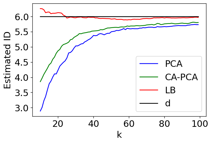
(b) Estimated ID for a 6-dimensional Lie group

Figure 2: Synthetic Manifolds in Higher Dimensions

The next example is a Lie group embedded in $\mathbb{R}^{15}$, constructed by taking the direct sum of the three-dimensional $SO(3)$ viewed as a subset of $\mathbb{R}^{3\times 3}\cong\mathbb{R}^{9}$ and the 3-torus viewed as a subset of $\mathbb{R}^{6}$ through the parameterization

$$(\theta_{1},\theta_{2},\theta_{3})\mapsto(\sin\theta_{1},\cos\theta_{1},\sin\theta_{2},\cos\theta_{2},\sin\theta_{3},\cos\theta_{3}).$$

Results for 20,000 randomly sampled points are depicted in Figure 2(b). CA-PCA fails to converge to the true dimension of 6, although it remains close even for small values of $k$ and outperforms PCA at every value of $k$ while competing with LB.

In Figure 2, we have plotted the average estimated dimension over a large number of points. Since there is plenty of “wiggle room” with the dimension and codimension so high, one may ask if the estimators consistently approximate the true dimension, or if they do so in the average only after providing alternating over- and underestimates. Figure 3 shows the standard deviation of the estimated dimensions for each test at fixed values of $k$. Since these are particularly small for both $SO(5)$ and $SO(3)\oplus\mathbb{T}^{3}$, the estimators, in particular PCA and CA-PCA, have consistently approximated the true ID in these cases.

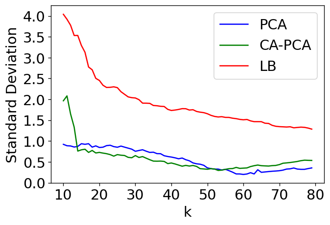
(a) Standard deviation of estimated ID for $SO(5)$

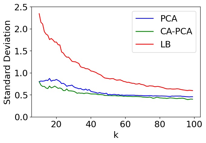
(b) Standard deviation of estimated ID for a 6-dimensional Lie group

Figure 3: Standard Deviation of Estimates for Synthetic Manifolds in Higher Dimensions

4.3 Some Simulated Data

An .stl file (3D image) of an airplane was rotated at a random angle around the $z$-axis before being projected onto the $x$-$z$ plane to determine a two-dimensional “photograph” of the airplane. Repeating this process, we obtained 200 images of size 432 by 288 pixels, viewed as vectors in $\mathbb{R}^{432\times 288}\cong\mathbb{R}^{124,416}$. (A similar approach was taken in [2].) The expected dimension of this point cloud is 1, given that the images were generated via a 1-dimensional group of symmetries. Results are depicted in Figure 4(a).

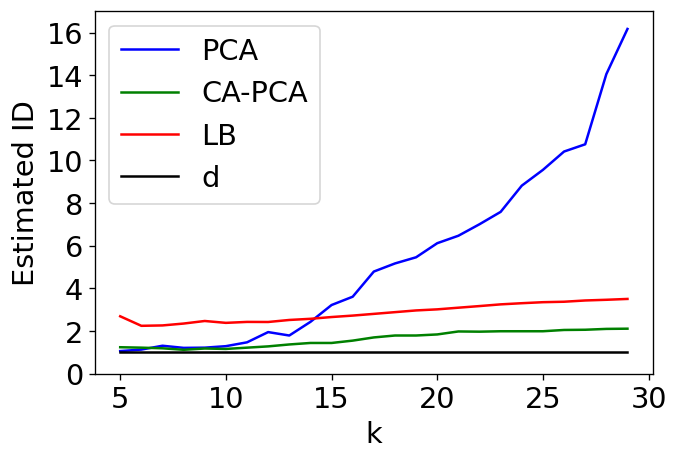
(a) Estimated ID for 1-D airplane photos, $N=100$

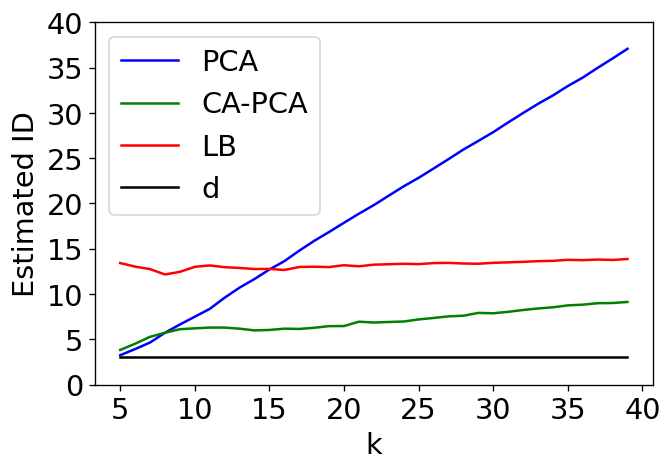
(b) Estimated ID for 3-D airplane photos, $N=100$

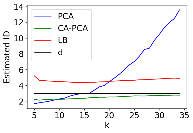
(c) Estimated ID for Isomap faces

Figure 4: Results for Simulated Data

As one can see, both PCA and CA-PCA provide close to the “correct” answer for small values of $k$; however, for $k>13$, the estimated dimension for PCA blows up while for CA-PCA it remains between 1 and approximately 2. Considering only PCA, one may suspect that the point cloud does not lie on or near a manifold, or consider an estimated dimension so far from the true value the estimator does not provide any benefits. In contrast, with CA-PCA the results are certainly consistent with data coming from a manifold. While the estimated dimension may be 2, a small amount of error assumed by the user might give them the range of 1 to 3, which may be sufficient.

We obtained 10,000 images of an airplane by applying a random element of $SO(3)$ (uniformly with respect to Haar measure) before projecting into two dimensions. The results of the ID estimators are shown in Figure 4(b). Here, it is clear that CA-PCA is not always able to magically estimate the dimension in such cases; however, it remains better than the other tests.

The Isomap face database consists of 698 greyscale images of size 64 by 64 pixels and has been used in [20, 23, 26] and many other works. The images are of an artificial face under varying illumination, vertical orientation, and horizontal orientation. Translating the images into vectors in $\mathbb{R}^{64\times 64}\cong\mathbb{R}^{4096}$, we obtain the results in Figure 4(c).

One may expect the true ID to be 3, due to the three parameters which vary in the construction of the photos. However, each of those three parameters has a clear upper and lower bound. For instance, there are photos with the head facing left, right, and center, but none with it facing backwards. By similar reasoning regarding the vertical orientation and brightness, we expect the Isomap faces to have similar structure as a three-dimensional unit cube.

The problem of determining the dimension of a manifold with boundary presents challenges distinct from those arising in dealing with manifolds without boundary. See [5, 10] for more on this problem.

For comparison, we construct a point cloud through random selection of 698 points from the unit cube in $\mathbb{R}^{3}$ and run the same tests, producing Figure 5(a). Here, all three tests give ID estimates less than 3. While this time it is CA-PCA which is highest and closest to 3, this still seems to suggest that we expect a dimension a little less than 3 for the Isomap faces.

(a) Estimated ID for unit cube in $\mathbb{R}^{3}$

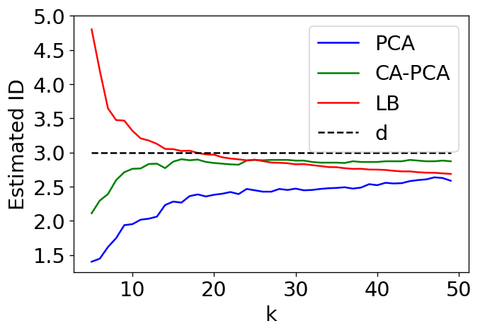
(b) Estimated ID for a rectangular prism

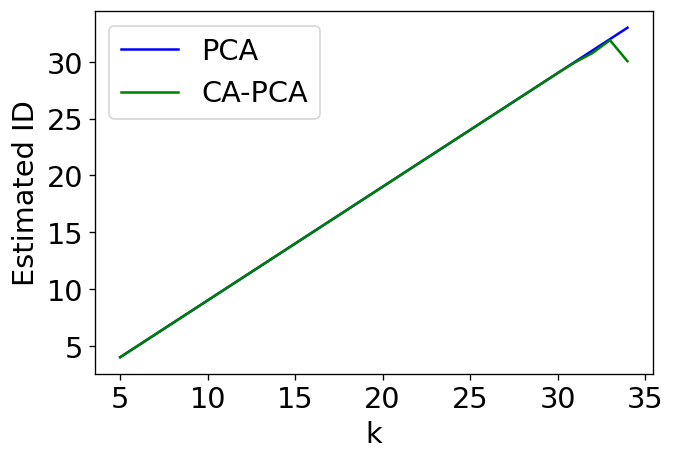
(c) Estimated ID for random images in $\mathbb{R}^{64\times 64}$

Figure 5: For Comparison with Isomap Faces

While the variations in the vertical and horizontal orientations of the face may be comparable in magnitude, it is unclear whether the variation in the brightness is the same. For this reason, we repeat the above with the unit cube replaced by $[0,1]\times[0,1]\times[0,5]$, with results in Figure 5(b). Again, the estimated dimensions is a little under 3.

We note that CA-PCA does tend to get closer to the ‘true’ dimension of 3, if one chooses to assign this value to a manifold with boundary. It is possible this is no coincidence; that given a sampled point at the center of a face of the unit cube, CA-PCA is better able to determine that the third and lowest eigenvalue is not due to curvature since this would require the first two eigenvalues to be smaller than observed. However, more investigation is needed to determine if CA-PCA truly analyzes manifolds with boundary differently.

Given the flexibility CA-PCA has to “move tail eigenvalues over to higher ones,” one may wonder if it is better able to estimate the dimension of the Isomap faces (and other sets of images) by consistent underestimation in the setting $k<<D$. To address this potential issue, we generated 698 random 64x64 grey-scale images (elements of the unit cube in $\mathbb{R}^{4096}$) and applied the three ID estimators. Results for PCA and CA-PCA are shown in Figure 5(c). (The LB estimator output values over 300 so its results are not depicted for readability of the graph.) Here, CA-PCA barely provides a lower estimate than PCA, suggesting its performance on the Isomap faces was truly due to proper estimation of the dimension rather than consistent underestimation.

4.4 Analysis of Non-Manifolds

Next, we see what happens when we apply the tests to another object which is not a manifold, in this case the union of two manifolds of different dimensions. We sample 200 points from the unit sphere in $\mathbb{R}^{4}$ and 200 points from the circle determined by the equations $(x_{1}-4)^{2}+x_{2}^{2}=16,x_{3}=0,x_{4}=0$. Running tests on the union of the two datasets gives Figure 6(a). Considering the average, it appears the estimators tend to a value of 2, the average of the dimension of the 3-sphere and that of the circle. However, the standard deviation of the estimates shown in Figure 6(b) demonstrates that there are many occurrences of 1’s and 3’s. For comparison, consider the standard deviations for the Klein bottle, shown in Figure 6(c).

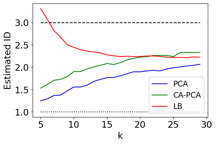
(a) Estimated ID for union of circle and $S^{3}$ with dimensions of circle (1) and $S^{3}$ (3)

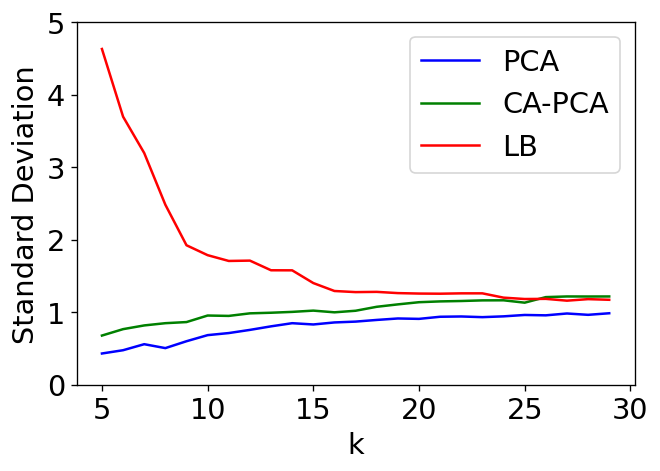
(b) Standard deviation of estimated ID for the union of circle and $S^{3}$

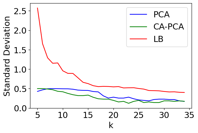
(c) Standard deviation of estimated ID for Klein bottle

Figure 6: Analysis of Non-Manifolds

Thus, CA-PCA, plus PCA and perhaps LB, may potentially assist in determining if data comes from a manifold.

4.5 Robustness to Error

Lastly, we test our estimator for robustness by introducing error into the samples. Error was added to each point by independently adding to each coordinate a random number sampled uniformly from the interval $(-\epsilon,\epsilon)$ for some choice of $\epsilon$. Figure 7(a) shows the results of the tests when this error was introduced to 400 points on the Klein bottle with $\epsilon=1$ (compare the results to those in Figure 1(a) and $\epsilon$ to the choice of $a=10,b=5$).

The same method was applied to 20,000 points from $SO(5)$ with $\epsilon=.1$, with the results depicted in Figure 7(b). In both cases of error, CA-PCA’s estimates are slightly further away from the true ID, yet still close and competitive with those from PCA. (Compare the results to those of Figure 2(a).)

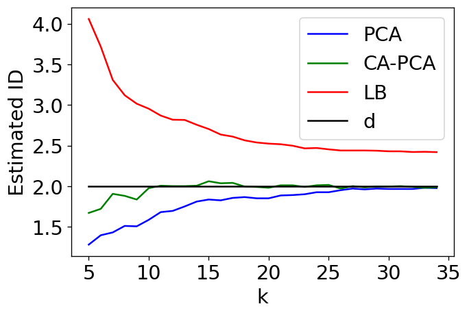
(a) Estimated ID for Klein bottle with error

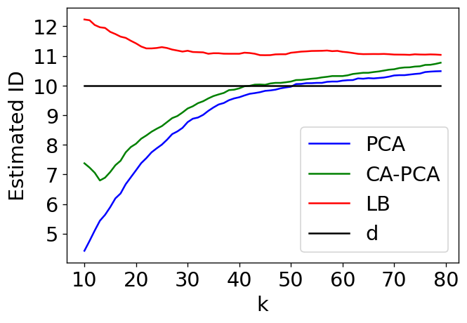
(b) Estimated ID for $SO(5)$ with error

Figure 7: Synthetic Manifolds with Error

5 Conclusion

As we have seen, the use of local PCA as an ID estimator may be improved in a variety of settings by taking into account curvature of the underlying manifold while generally providing good estimates and competing with LB.

CA-PCA is merely one of many potential applications of curvature analysis to ID estimators. In particular, calculations in the Appendix show that the $d$-dimensional volume of a ball of radius $r$ intersected with a $d$-dimensional manifold $\mathcal{M}$ is proportional to $r^{d}+cr^{d+2}$, where $c$ is a constant depending on $\mathcal{M}$ (see Subsection A.3). There are many ID estimators derived using a volume proportional to $r^{d}$ or related notions like average distances from the center of a ball. It would be interesting to see if any of these tests could be improved by taking curvature into account.

Another place for potential further study is that of ID estimation for manifolds with boundary. In our experiments, CA-PCA gets closer to the “true” ID of manifolds with boundary than PCA or LB, though more analysis is needed to determine if this is more than a coincidence.

Appendix A Integral Computations

A.1 Some Elementary Computations

Let $\sigma(x)$ denote the (non-normalized) surface measure on the sphere induced by Lebesgue measure on $\mathbb{R}^{d}$. We will often write $\sigma(x)$ when $x\in\mathbb{R}^{d}$ and $\sigma(\theta)$ when $\theta\in S^{d-1}$, the unit sphere in $\mathbb{R}^{d}$.

The following elementary fact can be found in [15], for instance.

Theorem A.1.

Let $P(x)=x_{1}^{\alpha_{1}}\cdots x_{d}^{\alpha_{d}}$ for $\alpha_{1},...,\alpha_{d}\in\{0,1,2,...\}$. Write $\beta_{j}=\frac{1}{2}(\alpha_{j}+1)$. Then, if all $\alpha_{j}$ are even,

$$\int_{S^{d-1}}P(x)d\sigma(x)=\frac{2\Gamma(\beta_{1})\cdots\Gamma(\beta_{d})}{\Gamma(\beta_{1}+...+\beta_{d})}.$$

If any $\alpha_{j}$ are odd, then the above integral is zero.

For our purposes, we will need the values $\Gamma(1/2)=\sqrt{\pi},\Gamma(3/2)=\frac{\sqrt{\pi}}{2},\Gamma(5/2)=\frac{3\sqrt{\pi}}{4},$ and $\Gamma(7/2)=\frac{15\sqrt{\pi}}{8}$ and the identity $\Gamma(x+1)=x\Gamma(x)$.

As particular instances of Theorem A.1,

$$\int_{S^{d-1}}d\sigma(x)=\frac{2\pi^{d/2}}{\Gamma(d/2)}$$ (17)

$$\int_{S^{d-1}}x_{i}^{2}d\sigma(x)=\frac{\pi^{d/2}}{\Gamma(d/2+1)}$$ (18)

$$\int_{S^{d-1}}x_{i}^{2}x_{j}^{2}d\sigma(x)=\frac{\pi^{d/2}}{2\Gamma(d/2+2)}$$ (19)

$$\int_{S^{d-1}}x_{i}^{4}d\sigma(x)=\frac{3\pi^{d/2}}{2\Gamma(d/2+2)}$$ (20)

$$\int_{S^{d-1}}x_{i}^{2}x_{j}^{2}x_{k}^{2}d\sigma(x)=\frac{\pi^{d/2}}{4\Gamma(d/2+3)}$$ (21)

$$\int_{S^{d-1}}x_{i}^{4}x_{j}^{2}d\sigma(x)=\frac{3\pi^{d/2}}{4\Gamma(d/2+3)}$$ (22)

$$\int_{S^{d-1}}x_{i}^{6}d\sigma(x)=\frac{15\pi^{d/2}}{4\Gamma(d/2+3)}$$ (23)

Lemma A.2.

Let $Q:\mathbb{R}^{d}\to\mathbb{R}$ be a quadratic form with eigenvalues $\mu_{1},...,\mu_{d}$. Then,

$$\int_{S^{d-1}}Q(\theta)d\theta=\frac{\pi^{d/2}}{\Gamma(d/2+1)}\sum_{k}\mu_{k}$$ (24)

Also,

$$\int_{S^{d-1}}Q(\theta)^{2}d\theta=\left(\frac{1}{2}\left(\sum_{k=1}^{d}\mu_{k}\right)^{2}+\sum_{k=1}^{d}\mu_{k}^{2}\right)\frac{\pi^{d/2}}{\Gamma(d/2+2)}.$$ (25)

Proof.

To establish (24), we rotate coordinates so the eigenvectors of $Q$ are $e_{1},...,e_{d}$ and use (18):

$$\int_{S^{d-1}}{Q}(\theta)d\theta =\int_{S^{d-1}}\sum_{k=1}^{d}\mu_{k}x_{k}^{2}d\theta$$

$$=\sum_{k=1}^{d}\mu_{k}\int_{S^{d-1}}x_{k}^{2}d\theta$$

$$=\frac{\sqrt{\pi}^{d}}{\Gamma(d/2+1)}\sum_{k=1}^{d}\mu_{k}.$$

For (25), we repeat the same rotation of coordinates and use (19) and (20):

$$\int_{S^{d-1}}Q(\theta)^{2}d\theta =\int_{S^{d-1}}\sum_{k=1}^{d}\mu_{k}x_{k}^{2}d\theta$$

$$=\sum_{1\leq k,l\leq d}\mu_{k}\mu_{l}\int_{S^{d-1}}x_{k}^{2}x_{l}^{2}d\theta$$

$$=\sum_{k=1}^{d}\mu_{k}^{2}\left[\frac{3}{2}\frac{\sqrt{\pi}^{d}}{\Gamma(d/2+2)}\right]+\sum_{k\neq l}\mu_{k}\mu_{l}\left[\frac{1}{2}\frac{\sqrt{\pi}^{d}}{\Gamma(d/2+2)}\right]$$

$$=\left(\frac{1}{2}(\sum_{k}\mu_{k})^{2}+\sum_{k}\mu_{k}^{2}\right)\frac{\sqrt{\pi}^{d}}{\Gamma(d/2+2)}$$

∎

A.2 The Region

First, let

$$q(x)=\sum_{j=1}^{D-d}Q_{j}(x)^{2}$$

and note $q(x)=O(\Lambda^{2})$ for $|x|\leq 1$.

Writing $x=r\theta$, with $r\geq 0$ and $\theta\in S^{d-1}$, let $r=r(\theta)$ denote the positive real solution to

$$r^{2}+q(r\theta)=r^{2}+r^{4}q(\theta)=1.$$

By the quadratic formula and Taylor expansion $\sqrt{1+t}=1+\frac{t}{2}+O(t^{2})$,

$$r^{2}(\theta) =\frac{-1+\sqrt{1+4q(\theta)}}{2q(\theta)}$$

$$=\frac{-1+1+2q(\theta)-2q(\theta)^{2}+O(q(\theta)^{3})}{2q(\theta)}$$

$$=1-q(\theta)+O(\Lambda^{4}).$$

Thus,

$$r(\theta)=1-\frac{q(\theta)}{2}+O(\Lambda^{4}).$$ (26)

and

$$r(\theta)^{m}=1-\frac{mq(\theta)}{2}+O(\Lambda^{4}).$$ (27)

This approximation will be used throughout this section as we integrate over spherical coordinates $(r,\theta)$ and need to find the limits of our integral in $r$.

A.3 Total Surface Area

To begin the computation of the volume of $\mathcal{M}\cap B_{1}(0)$, we switch to polar coordinates, substitute the expression of $S(x)$ in (2), and integrate with respect to the radius

$$\int_{R}S(x)dx =\int_{S^{d-1}}\int_{0}^{r(\theta)}S(r\theta)r^{d-1}drd\theta$$

$$=\int_{S^{d-1}}\int_{0}^{r(\theta)}\left(1+2\sum_{j=1}^{D-d}\tilde{Q}_{j}(r\theta)\right)r^{d-1}drd\theta+O(\Lambda^{4})$$

$$=\int_{S^{d-1}}\int_{0}^{r(\theta)}r^{d-1}+2r^{d+1}\sum_{j=1}^{D-d}\tilde{Q}_{j}(\theta)drd\theta$$

$$=\int_{S^{d-1}}\frac{1}{d}r(\theta)^{d}+\frac{2}{d+2}r(\theta)^{d+2}\sum_{j=1}^{D-d}\tilde{Q}_{j}(\theta)d\theta.$$

By (27),

$$\int_{R}S(x)dx =\int_{S^{d-1}}\frac{1}{d}(1-\frac{dq(\theta)}{2})+\frac{2}{d+2}(1-\frac{(d+2)q(\theta)}{2})\sum_{j=1}^{D-d}\tilde{Q}_{j}(\theta)d\theta+O(\Lambda^{4})$$

$$=\int_{S^{d-1}}\frac{1}{d}-\frac{q(\theta)}{2}+\frac{2}{d+2}\sum_{j=1}^{D-d}\tilde{Q}_{j}(\theta)d\theta+O(\Lambda^{4})$$

By (17), (24), and (25), we integrate over $S^{d-1}$ and find

$$\int_{R}S(x)dx= \frac{2\pi^{d/2}}{d\Gamma(d/2)}-\frac{\pi^{d/2}}{2\Gamma(d/2+2)}\sum_{j}\left(\frac{1}{2}(\sum_{k}\lambda_{j,k})^{2}+\sum_{k}\lambda_{j,k}^{2}\right)$$

$$+\frac{2\pi^{d/2}}{(d+2)\Gamma(d/2+1)}\sum_{j,k}\lambda_{j,k}^{2}+O(\Lambda^{4})$$

$$= \frac{\pi^{d/2}}{\Gamma(d/2)}\left[\frac{2}{d}-\frac{2}{(d+2)(d+4)}\left(A+\frac{1}{2}B\right)+\frac{4}{(d+2)^{2}}A\right]+O(\Lambda^{4})$$

$$= \frac{\pi^{d/2}}{\Gamma(d/2)}\left[\frac{2}{d}-\frac{1}{(d+2)(d+4)}B+\frac{2(d+6)}{(d+2)^{2}(d+4)}A\right]+O(\Lambda^{4})$$

A.4 Normalizing with Respect to Surface Area

In this subsection, we take a quick detour to show how Taylor series expansion will be used to divide by $\int_{R}S(x)dx$ in normalizing the relevant integrals.

note how division by total surface area will occur.

We use the expansion

$$\frac{a_{0}+a_{1}t+O(t^{2})}{b_{0}+b_{1}t+O(t^{2})} =\left(\frac{a_{0}}{b_{0}}+\frac{a_{1}}{b_{0}}t+O(t^{2})\right)\frac{1}{1+\frac{b_{1}}{b_{0}}t+O(t^{2})}$$ (28)

$$=\left(\frac{a_{0}}{b_{0}}+\frac{a_{1}}{b_{0}}t+O(t^{2})\right)\left(1-\frac{b_{1}}{b_{0}}t+O(t^{2})\right)$$ (29)

$$=\frac{a_{0}}{b_{0}}+\frac{a_{1}}{b_{0}}t-\frac{a_{0}b_{1}}{b_{0}^{2}}t+O(t^{2})$$ (30)

to estimate these ratios (matching $t$ with $\Lambda^{2}$, roughly)

A.5 The Means

By Lemma 3.1 and integrating in the radial direction,

$$\int_{R}Q_{i}(x)S(x)dx =\int_{S^{d-1}}\int_{0}^{r(\theta)}Q_{i}(x)\left[r^{d-1}+2r^{d+1}\sum_{j=1}^{D-d}\tilde{Q}_{j}(\theta)\right]\left(1+2\sum_{j=1}^{D-d}\tilde{Q}_{j}(r\theta)\right)drd\theta$$

$$+O(\Lambda^{4})$$

$$= \int_{S^{d-1}}\int_{0}^{r(\theta)}Q_{i}(x)r^{d-1}drd\theta+O(\Lambda^{3})$$

$$= \int_{S^{d-1}}\int_{0}^{r(\theta)}r^{d+1}Q_{i}(\theta)drd\theta+O(\Lambda^{3})$$

$$= \int_{S^{d-1}}\frac{1}{d+2}Q_{i}(\theta)r(\theta)^{d+2}d\theta+O(\Lambda^{3}).$$

Thus, applying (27) and (24),

$$\int_{R}Q_{i}(x)S(x)dx =\int_{S^{d-1}}\frac{1}{d+2}Q_{i}(\theta)d\theta+O(\Lambda^{3})$$

$$=\frac{\pi^{d/2}}{(d+2)\Gamma(d/2+1)}\sum_{j=1}^{d}\lambda_{i,j}+O(\Lambda^{3}).$$

Upon normalizing, we find

$$\bar{Q}_{i}=\frac{\int_{R}Q_{i}(x)S(x)dx}{\int_{R}S(x)dx}=\frac{1}{d+2}\sum_{j=1}^{d}\lambda_{i,j}+O(\Lambda^{2}).$$

Note that we only need this computation up to first-order accuracy since we will only need the above expression to multiply it by other terms depending on $\Lambda$ in the computation of $I_{4}$.

A.6 Upper Trace

Let $\theta^{*}\in S^{d-1}$ be arbitrary. We begin as with the computation of total surface area, converting to polar coordinates and integrating in $r$ first to get

$$\int_{R}(x\cdot\theta^{*})^{2}S(x)dx =\int_{S^{d-1}}\int_{0}^{r(\theta)}(r\theta\cdot\theta^{*})^{2}\left[r^{d-1}+2r^{d+1}\sum_{j=1}^{D-d}\tilde{Q}_{j}(\theta)\right]drd\theta+O(\Lambda^{4})$$

$$=\int_{S^{d-1}}(\theta\cdot\theta^{*})^{2}\int_{0}^{r(\theta)}r^{d+1}+2r^{d+3}\sum_{j=1}^{D-d}\tilde{Q}_{j}(\theta)drd\theta+O(\Lambda^{4})$$

$$=\int_{S^{d-1}}(\theta\cdot\theta^{*})^{2}\left[\frac{1}{d+2}r(\theta)^{d+2}+\frac{2}{d+4}r(\theta)^{d+4}\sum_{j=1}^{D-d}\tilde{Q}_{j}(\theta)\right]d\theta+O(\Lambda^{4})$$

By (27), may rewrite the above as

$$\int_{S^{d-1}}(\theta\cdot\theta^{*})^{2}\left[\frac{1}{d+2}(1-\frac{(d+2)q(\theta)}{2})+\frac{2}{d+4}(1-\frac{(d+4)q(\theta)}{2})\sum_{j=1}^{D-d}\tilde{Q}_{j}(\theta)\right]d\theta+O(\Lambda^{4}),$$ (31)

or

$$\int_{R}(x\cdot\theta^{*})^{2}S(x)dx=\int_{S^{d-1}}(\theta\cdot\theta^{*})^{2}\left[\frac{1}{d+2}-\frac{q(\theta)}{2}+\frac{2}{d+4}\sum_{j=1}^{D-d}\tilde{Q}_{j}(\theta)\right]d\theta+O(\Lambda^{4})$$ (32)

By taking $\theta^{*}=e_{i}$ ($1\leq i\leq d$) and summing over $i$, we obtain the sum of the first $d$ eigenvalues. By the identity $\sum_{i=1}^{d}(\theta\cdot e_{i})^{2}=1$ for $\theta\in S^{d-1}$, we have

$$\sum_{i}I_{1}(i)= \int_{S^{d-1}}\left[\frac{1}{d+2}-\frac{q(\theta)}{2}+\frac{2}{d+4}\sum_{j=1}^{D-d}\tilde{Q}_{j}(\theta)\right]d\theta+O(\Lambda^{4})$$

$$= \frac{2\pi^{d/2}}{(d+2)\Gamma(d/2)}-\frac{\pi^{d/2}}{2\Gamma(d/2+2)}\sum_{j}\left(\frac{1}{2}(\sum_{k}\lambda_{j,k})^{2}+\sum_{k}\lambda_{j,k}^{2}\right)$$

$$+\frac{2\pi^{d/2}}{(d+4)\Gamma(d/2+1)}\sum_{j,k}\lambda_{j,k}^{2}+O(\Lambda^{4})$$

$$= \frac{\pi^{d/2}}{\Gamma(d/2)}\left[\frac{2}{d+2}-\frac{1}{d(d+2)}B+\frac{2}{(d+2)(d+4)}A\right]+O(\Lambda^{4}).$$

To complete our computation of the upper trace, we divide by the total surface area

$$\sum_{i}\frac{I_{1}(i)}{V}= \frac{\frac{\pi^{d/2}}{\Gamma(d/2)}\left[\frac{2}{d+2}-\frac{1}{d(d+2)}B+\frac{2}{(d+2)(d+4)}A\right]+O(\Lambda^{4})}{\frac{\pi^{d/2}}{\Gamma(d/2)}\left[\frac{2}{d}-\frac{1}{(d+2)(d+4)}B+\frac{2(d+6)}{(d+2)^{2}(d+4)}A\right]+O(\Lambda^{4})}$$

$$= \frac{d}{d+2}-\frac{1}{2(d+2)}B+\frac{d}{(d+2)(d+4)}A+\frac{d^{2}}{2(d+2)^{2}(d+4)}B-\frac{d^{2}(d+6)}{(d+2)^{3}(d+4)}A$$

$$+O(\Lambda^{4})$$

$$= \frac{d}{d+2}+\frac{4d-2d^{2}}{(d+2)^{3}(d+4)}A-\frac{3d+4}{(d+2)^{2}(d+4)}B+O(\Lambda^{4}).$$

A.7 Bounds for Upper Eigenvalues

Here, we will determine the lower and upper bounds for the eigenvalues of $\Sigma_{1}$ (found in (10) and (11) by approximating the expression in (32) without particular choice of $\theta^{*}$.

Fix $1\leq j\leq D-d$ and perform a rotation so the eigenvectors of $\tilde{Q}_{j}$ to be $e_{1},...,e_{d}$ (keeping $\theta^{*}=(y_{1},...,y_{d})$ arbitrary). By ignoring any terms with odd degrees of $x_{k}$ and applying (19) and (20)

$$\int_{S^{d-1}}(\theta\cdot y)^{2}\tilde{Q}_{j}(\theta)d\theta =\sum_{k}^{d}y_{k}^{2}\lambda_{j,k}^{2}\int_{S^{d-1}}x_{k}^{4}dx+\sum_{k\neq l}y_{k}^{2}\lambda_{j,l}^{2}\int_{S^{d-1}}x_{k}^{2}x_{l}^{2}dx$$ (33)

$$=\sum_{k}y_{k}^{2}\lambda_{j.k}^{2}\left(\frac{3}{2}\frac{\pi^{d/2}}{\Gamma(d/2+2)}\right)+\sum_{k\neq l}y_{k}^{2}\lambda_{j,l}^{2}\left(\frac{1}{2}\frac{\pi^{d/2}}{\Gamma(d/2+2)}\right)$$ (34)

$$\leq\sum_{k}y^{2}_{k}\sum_{l}\lambda_{j,l}^{2}\left(\frac{3}{2}\frac{\pi^{d/2}}{\Gamma(d/2+2)}\right)$$ (35)

$$=\frac{3}{2}\frac{\pi^{d/2}}{\Gamma(d/2+2)}\sum_{k}\lambda_{j,k}^{2}$$ (36)

Similarly,

$$\int_{S^{d-1}}(\theta\cdot y)^{2}\tilde{Q}_{j}(\theta)d\theta\geq\frac{1}{2}\frac{\pi^{d/2}}{\Gamma(d/2+2)}\sum_{k}\lambda_{j,k}^{2}.$$ (37)

Repeating the above strategy, we bound

$$\int_{S^{d-1}}(\theta\cdot y)^{2}Q_{j}(\theta)^{2}d\theta=\int_{S^{d-1}}\left(\sum_{k=1}^{d}y_{k}^{2}x_{k}^{2}\right)\left(\sum_{l=1}^{d}\lambda_{j,l}x_{l}^{2}\right)\left(\sum_{m=1}^{d}\lambda_{j,m}x_{m}^{2}\right)d\theta.$$

Expanding the above and applying (21), (22), and (23) gives

$$\frac{\pi^{d/2}}{\Gamma(d/2+3)}\left(\sum_{k}\frac{15y_{k}^{2}\lambda_{j,k}^{2}}{4}+\sum_{k\neq l\neq m\neq k}\frac{y_{k}^{2}\lambda_{j,l}\lambda_{j,m}}{4}+2\sum_{k\neq l}\frac{3y_{k}^{2}\lambda_{j,k}\lambda_{j,l}}{4}+\sum_{k\neq l}\frac{3y_{k}^{2}\lambda_{j,l}^{2}}{4}\right).$$

Thus,

$$\int_{S^{d-1}}(\theta\cdot y)^{2}Q_{j}(\theta)^{2}d\theta \leq\frac{\pi^{d/2}}{\Gamma(d/2+3)}\left(\sum_{k}\frac{15y_{k}^{2}}{4}\sum_{l}\lambda_{j,l}^{2}+\sum_{k}y_{k}^{2}\frac{3}{2}\left((\sum_{l}\lambda_{j,l})^{2}+\sum_{l}\lambda_{j,l}^{2}\right)\right)$$ (38)

$$=\frac{\pi^{d/2}}{\Gamma(d/2+3)}\left(\frac{21}{4}\sum_{l}\lambda_{j,l}^{2}+\frac{3}{2}(\sum_{l}\lambda_{j,l})^{2}\right)$$ (39)

Here, we simply acknowledge

$$\int_{S^{d-1}}(\theta\cdot y)^{2}Q_{j}(\theta)^{2}d\theta\geq 0.$$ (40)

Subbing (36) and (40) into (32), we find

$$\int_{R}(x\cdot\theta^{*})^{2}S(x)dx \leq\int_{S^{d-1}}(\theta\cdot\theta^{*})^{2}\frac{1}{d+2}d\theta+\frac{2}{d+4}\frac{3}{2}\frac{\pi^{d/2}}{\Gamma(d/2+2)}\sum_{j,k}\lambda_{j,k}^{2}+O(\Lambda^{4})$$

$$=\int_{S^{d-1}}x_{1}^{2}\frac{1}{d+2}d\theta+\frac{3}{d+4}\frac{\pi^{d/2}}{\Gamma(d/2+2)}A+O(\Lambda^{4})$$

$$=\frac{1}{d+2}\frac{\pi^{d/2}}{\Gamma(d/2+1)}+\frac{3}{d+4}\frac{\pi^{d/2}}{\Gamma(d/2+2)}A+O(\Lambda^{4})$$

$$=\frac{\pi^{d/2}}{\Gamma(d/2)}\left[\frac{2}{d(d+2)}+\frac{12}{d(d+2)(d+4)}A\right]+O(\Lambda^{4})$$

To normalize the upper bound we divide the above by $V$ to get

$$\frac{\int_{R}(x\cdot\theta^{*})^{2}S(x)dx}{\int_{R}S(x)dx} \leq\frac{\frac{\pi^{d/2}}{\Gamma(d/2)}\left[\frac{2}{d(d+2)}+\frac{12}{d(d+2)(d+4)}A\right]+O(\Lambda^{4})}{\frac{\pi^{d/2}}{\Gamma(d/2)}\left[\frac{2}{d}-\frac{1}{(d+2)(d+4)}B+\frac{2(d+6)}{(d+2)^{2}(d+4)}A\right]+O(\Lambda^{4})}$$

$$=\frac{1}{d+2}+\frac{6}{(d+2)(d+4)}A$$

$$-\frac{1}{d+2}\left[-\frac{d}{2(d+2)(d+4)}B+\frac{d(d+6)}{(d+2)^{2}(d+4)}A\right]+O(\Lambda^{4})$$

$$=\frac{1}{d+2}+\frac{5d^{2}+18d+24}{(d+2)^{3}(d+4)}A+\frac{d}{2(d+2)^{2}(d+4)}B+O(\Lambda^{4})$$

Subbing (37) and (39) into (32), we see

$$\int_{R}(x\cdot\theta^{*})^{2}S(x)dx \geq\frac{1}{d+2}\frac{\pi^{d/2}}{\Gamma(d/2+1)}-\frac{\pi^{d/2}}{\Gamma(d/2+3)}\left(\frac{21}{4}\sum_{j}\sum_{l}\lambda_{j,l}^{2}+\frac{3}{2}\sum_{j}(\sum_{l}\lambda_{j,l})^{2}\right)$$

$$+\frac{1}{d+4}\frac{\pi^{d/2}}{\Gamma(d/2+2)}\sum_{j}\sum_{k}\lambda_{j,k}^{2}+O(\Lambda^{4})$$

$$=\frac{1}{d+2}\frac{\pi^{d/2}}{\Gamma(d/2+1)}-\frac{\pi^{d/2}}{\Gamma(d/2+3)}\left(\frac{21}{4}A+\frac{3}{2}B\right)$$

$$+\frac{\pi^{d/2}}{\Gamma(d/2+3)}\frac{1}{2}A+O(\Lambda^{4})$$

$$=\frac{\pi^{d/2}}{\Gamma(d/2)}\left[\frac{2}{d(d+2)}-\frac{8}{d(d+2)(d+4)}\left(\frac{19}{4}A+\frac{3}{2}B\right)\right]+O(\Lambda^{4}).$$

To obtain the lower bound on the eigenvalues, we divide by total surface area:

$$\frac{\int_{R}(x\cdot\theta^{*})^{2}S(x)dx}{\int_{R}S(x)dx}\geq \frac{\frac{2}{d(d+2)}-\frac{8}{d(d+2)(d+4)}\left(\frac{19}{4}A+\frac{3}{2}B\right)+O(\Lambda^{4})}{\frac{2}{d}-\frac{1}{(d+2)(d+4)}B+\frac{2(d+6)}{(d+2)^{2}(d+4)}A+O(\Lambda^{4})}$$

$$= \frac{1}{d+2}-\frac{19}{(d+2)(d+4)}A-\frac{6}{(d+2)(d+4)}B+\frac{d}{2(d+2)^{2}(d+4)}B$$

$$-\frac{d(d+6)}{(d+2)^{3}(d+4)}A+O(\Lambda^{4})$$

$$= \frac{1}{d+2}-\frac{20d^{2}+82d+76}{(d+2)^{3}(d+4)}A-\frac{11d+24}{2(d+2)^{2}(d+4)}B+O(\Lambda^{4})$$

A.8 Lower Eigenvalues

We repeat the strategy of prior computations, taking advantage of the fact that $Q_{j}(x)^{2}-\bar{Q}_{j}^{2}=O(\Lambda^{2})$ so the $O(\Lambda^{2})$ terms in $S(x)$ turn into higher-order error. Similarly, we are able to take $r(\theta)\approx 1$ once we have integrated in $r$.

$$\int_{R}(Q_{j}(x)^{2}-\bar{Q}_{j}^{2})S(x)dx =\int_{R}Q_{j}(x)^{2}-\bar{Q}_{j}^{2}dx+O(\Lambda^{4})$$

$$=\int_{S^{d-1}}\int_{0}^{r(\theta)}r^{d-1}\left[r^{2}Q_{j}(\theta)^{2}-\bar{Q}_{j}^{2}\right]drd\theta+O(\Lambda^{4})$$

$$=\int_{S^{d-1}}\frac{1}{d+2}r(\theta)^{d+2}Q_{j}(\theta)^{2}-\frac{1}{d}r(\theta)^{d}\bar{Q}_{j}^{2}d\theta+O(\Lambda^{4})$$

$$=\int_{S^{d-1}}\frac{1}{d+2}Q_{j}(\theta)^{2}-\frac{1}{d}\bar{Q}_{j}^{2}d\theta+O(\Lambda^{4})$$

By Lemma A.2 and substituting our value of $\bar{Q}_{i}$,

$$\int_{R}(Q_{j}(x)^{2}-\bar{Q}_{j}^{2})S(x)dx= \left(\frac{1}{2(d+2)}(\sum_{k}\lambda_{j,k})^{2}+\frac{1}{d+2}\sum_{k}\lambda_{j,k}^{2}\right)\frac{\pi^{d/2}}{\Gamma(d/2+2)}$$

$$-\frac{1}{d}\frac{2\pi^{d/2}}{\Gamma(d/2)}\left(\bar{Q}_{i}\right)^{2}+O(\Lambda^{3})$$

$$= \left(\frac{1}{2(d+2)}(\sum_{k}\lambda_{j,k})^{2}+\frac{1}{d+2}\sum_{k}\lambda_{j,k}^{2}\right)\frac{\pi^{d/2}}{\Gamma(d/2+2)}$$

$$-\frac{1}{d}\frac{2\pi^{d/2}}{\Gamma(d/2)}\left(\frac{1}{d+2}\sum_{j=1}^{d}\lambda_{i,j}+O(\Lambda^{2})\right)^{2}+O(\Lambda^{3})$$

$$= \frac{\pi^{d/2}}{\Gamma(d/2)}\left[\frac{2}{d(d+2)^{2}}B_{j}+\frac{4}{d(d+2)^{2}}A_{j}-\frac{2}{d(d+2)^{2}}B_{j}\right]+O(\Lambda^{3})$$

$$= \frac{\pi^{d/2}}{\Gamma(d/2)}\frac{4}{d(d+2)^{2}}A_{j}+O(\Lambda^{3}).$$

We normalize to get

$$\frac{\int_{R}(Q_{i}(x)-\bar{Q}_{i})^{2}S(x)dx}{\int_{R}S(x)dx} =\frac{\frac{4}{d(d+2)^{2}}A_{j}+O(\Lambda^{3})}{\frac{2}{d}-\frac{1}{(d+2)(d+4)}B+\frac{2(d+6)}{(d+2)^{2}(d+4)}A+O(\Lambda^{4})}$$

$$=\frac{2}{(d+2)^{2}}A_{j}+O(\Lambda^{3}).$$

Lastly, summing over $i$ gives (9).

References

• [1] Eddie Aamari and Clรฉment Levrard. Nonasymptotic rates for manifold, tangent space and curvature estimation. The Annals of Statistics, 47(1):177โ€“204, 2019.
• [2] Yariv Aizenbud and Barak Sober. Non-parametric estimation of manifolds from noisy data. arXiv preprint arXiv:2105.04754, 2021.
• [3] Ege Altan, Saraย A Solla, Leeย E Miller, and Ericย J Perreault. Estimating the dimensionality of the manifold underlying multi-electrode neural recordings. PLoS computational biology, 17(11):e1008591, 2021.
• [4] Richardย G Baraniuk and Michaelย B Wakin. Random projections of smooth manifolds. Foundations of Computational Mathematics, 9(1):51โ€“77, 2009.
• [5] Tyrus Berry and Timothy Sauer. Density estimation on manifolds with boundary. Computational Statistics & Data Analysis, 107:1โ€“17, 2017.
• [6] Adam Block, Zeyu Jia, Yury Polyanskiy, and Alexander Rakhlin. Intrinsic dimension estimation using wasserstein distance. Journal of Machine Learning Research, 23(313):1โ€“37, 2022.
• [7] Charles Bouveyron, Gilles Celeux, and Stรฉphane Girard. Intrinsic dimension estimation by maximum likelihood in isotropic probabilistic PCA. Pattern Recognition Letters, 32(14):1706โ€“1713, 2011.
• [8] Francesco Camastra and Antonino Staiano. Intrinsic dimension estimation: Advances and open problems. Information Sciences, 328:26โ€“41, 2016.
• [9] P.ย Campadelli, E.ย Casiraghi, C.ย Ceruti, and A.ย Rozza. Intrinsic dimension estimation: relevant techniques and a benchmark framework. Math. Probl. Eng., pages Art. ID 759567, 21, 2015.
• [10] Kevinย M Carter, Alfredย O Hero, and Raviv Raich. De-biasing for intrinsic dimension estimation. In 2007 IEEE/SP 14th Workshop on Statistical Signal Processing, pages 601โ€“605. IEEE, 2007.
• [11] Frรฉdรฉric Cazals and Marc Pouget. Estimating differential quantities using polynomial fitting of osculating jets. Computer Aided Geometric Design, 22(2):121โ€“146, 2005.
• [12] Chun-houh Chen, Wolfgang Hรคrdle, Antony Unwin, Michaelย AA Cox, and Trevorย F Cox. Multidimensional scaling. Handbook of data visualization, pages 315โ€“347, 2008.
• [13] Kennethย L Clarkson. Tighter bounds for random projections of manifolds. In Proceedings of the twenty-fourth annual symposium on Computational geometry, pages 39โ€“48, 2008.
• [14] Francesco Denti, Diego Doimo, Alessandro Laio, and Antonietta Mira. Distributional results for model-based intrinsic dimension estimators. arXiv preprint arXiv:2104.13832, 2021.
• [15] Geraldย B. Folland. How to integrate a polynomial over a sphere. Amer. Math. Monthly, 108(5):446โ€“448, 2001.
• [16] Stephenย L France and Jย Douglas Carroll. Two-way multidimensional scaling: A review. IEEE Transactions on Systems, Man, and Cybernetics, Part C (Applications and Reviews), 41(5):644โ€“661, 2010.
• [17] Keinosuke Fukunaga and Davidย R Olsen. An algorithm for finding intrinsic dimensionality of data. IEEE Transactions on Computers, 100(2):176โ€“183, 1971.
• [18] Lucient Grillet and Juan Souto. Effective estimation of the dimensions of a manifold from random samples. arXiv preprint arXiv:2209.01839, 2022.
• [19] Yue Guan and Jennifer Dy. Sparse probabilistic principal component analysis. In Artificial Intelligence and Statistics, pages 185โ€“192. PMLR, 2009.
• [20] Elizaveta Levina and Peter Bickel. Maximum likelihood estimation of intrinsic dimension. Advances in neural information processing systems, 17, 2004.
• [21] Didong Li, Minerva Mukhopadhyay, and Davidย B. Dunson. Efficient manifold approximation with spherelets. J. R. Stat. Soc. Ser. B. Stat. Methodol., 84(4):1129โ€“1149, 2022.
• [22] Uzu Lim, Vidit Nanda, and Harald Oberhauser. Tangent space and dimension estimation with the Wasserstein distance. arXiv preprint arXiv:2110.06357, 2021.
• [23] Tong Lin and Hongbin Zha. Riemannian manifold learning. IEEE transactions on pattern analysis and machine intelligence, 30(5):796โ€“809, 2008.
• [24] Annaย V Little, Jason Lee, Yoon-Mo Jung, and Mauro Maggioni. Estimation of intrinsic dimensionality of samples from noisy low-dimensional manifolds in high dimensions with multiscale SVD. In 2009 IEEE/SP 15th Workshop on Statistical Signal Processing, pages 85โ€“88. IEEE, 2009.
• [25] Edgar Santos-Fernandez, Francesco Denti, Kerrie Mengersen, and Antonietta Mira. The role of intrinsic dimension in high-resolution player tracking dataโ€”insights in basketball. The Annals of Applied Statistics, 16(1):326โ€“348, 2022.
• [26] Joshuaย B Tenenbaum, Vinย de Silva, and Johnย C Langford. A global geometric framework for nonlinear dimensionality reduction. science, 290(5500):2319โ€“2323, 2000.
• [27] Hemant Tyagi, Elฤฑf Vural, and Pascal Frossard. Tangent space estimation for smooth embeddings of Riemannian manifolds. Information and Inference: A Journal of the IMA, 2(1):69โ€“114, 2013.
• [28] Laurens Vanย der Maaten and Geoffrey Hinton. Visualizing data using t-sne. Journal of machine learning research, 9(11), 2008.
• [29] Peterย J. Verveer and Robert P.ย W. Duin. An evaluation of intrinsic dimensionality estimators. IEEE Transactions on pattern analysis and machine intelligence, 17(1):81โ€“86, 1995.