Dynamical Gravastar “Simulated Horizon” from TOV Equation Initial Value Problem with Relativistic Matter

Abstract

We continue the study of “dynamical gravastars”, constructed by solving the Tolman-Oppenheimer-Volkoff (TOV) equation with relativistic matter, undergoing a phase transition at high pressure to a state with negative energy density, as allowed in quantum theory. Since generation of a horizon-like structure or “simulated horizon” occurs at a radius above where the phase transition occurs, it is solely a property of the TOV equation with relativistic matter, for appropriate small radius initial conditions. We survey the formation of a simulated horizon from this point of view. From the numerical solutions, we show that the metric exponent appearing in the TOV equation undergoes an arc tangent-like jump, leading to formation of the simulated horizon. Rescaling the problem to fixed initial radius, we plot the “phase diagram” in the initial pressure–initial mass plane, showing the range of parameters where a simulated horizon dynamically forms.

I Are astrophysical black holes mathematical black holes, or dynamical gravastars?

Observations by the EHT eht of Sg A* and M87 confirm that each has the expected exterior spacetime geometry of a black hole of mass $M$, with a light sphere at a radius $3M$ lying outside the Schwarzschild radius of $2M$. A key question that remains is whether what lies inside the light sphere is a true mathematical black hole, or a novel type of relativistic star or “exotic compact object” pani ? Two recent papers adler1 , adler2 have presented a theory of “dynamical gravastars”, based on using as input only the Tolman-Oppenheimer-Volkoff (TOV) equations, and an assumed equation of state, with continuous pressure $p\geq 0$ and a jump in the energy density $\rho$ at a pressure pjump, from an external relativistic matter state with $\rho=3p$ to an interior state with $p+\rho=\beta$, where $0<\beta<<1$.

The second paper adler2 introduced two simplifications into the model constructed in adler1 , by setting the cosmological constant to zero (which has a negligible effect on the numerical results) and by replacing the smoothed sigmoidal function used for the energy density jump in adler1 with a step function jump (which changes numerical results but leaves qualitative features unaltered). We shall use the simplified version of the model in this paper, since as discussed in adler2 , in addition to eliminating two superfluous parameters from the gravastar model, it greatly simplifies tuning the initial value of the metric exponent $\nu$, and thus facilitate surveys over the model parameter space.

II The gravastar simulated horizon is a property of the TOV eqution for relativistic matter

A typical result obtained from the simplified model is shown in Fig. 1, where we have plotted the denominator function $denom=1-2m(r)/r$ appearing in the TOV equations written below, with $m(r)$ the volume integrated energy density. This graph was plotted with parameters $\beta=.01$ and pjump=.95. From this graph we see that the energy density jump, which occurs at a radius $r\simeq 48.895$, occurs well inside the kink structure around the simulated horizon, which lies at the radius $r\simeq 59.43754$. Hence the kink structure and generation of the simulated horizon are entirely a property of the TOV equation with relativistic matter and continuous pressure and density, when supplied appropriate initial values at the inner radius where the energy density jump occurs. This is the viewpoint from which we will study the dynamical gravastar model in the present paper. Just to check that our use of the term “simulated horizon” is appropriate, in Fig. 2 we plot $g_{00}(r)=e^{\nu(r)}$ from the dynamical gravastar calculation used in Fig. 1. This is nearly indistinguishable from the exterior Schwarzschild geometry for a black hole of mass $M=29.721$. However, the logarithmic plot in Fig. 3 shows that within the simulated horizon, $g_{00}$ for the dynamical gravastar remains always positive, but becomes very small. This means that objects that enter the simulated horizon can get back out, but with potentially very large time delays. If astrophysical black holes are gravastars, this could explain the recent report by Cendes et al. cendes that many black hole tidal disruption events have subsequent radio emissions delayed by hundreds to thousands of days.

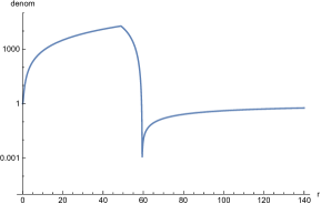
Figure 1: Plot of $denom$ for the TOV.01 notebook. The energy density jump at $r=48.895$ is apparent; above this radius the functions entering the TOV equations are continuous.

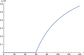
Figure 2: Plot of $g_{00}$ for the same parameters used in Fig. 1. Outside the radius $r\simeq 59.44$, this plot is nearly indistinguishable from a plot of the exterior Schwarzschild geometry for a black hole of mass $M=29.721$.

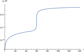
Figure 3: Log plot of $g_{00}$ for the same parameters used in Fig. 1. This shows that $g_{00}$ is always positive within the simulated horizon, but becomes very small.

III TOV equation system governing dynamical gravastars, and its rescaling covariance

The TOV equations as given in adler2 are

$$\frac{dm(r)}{dr}= 4\pi r^{2}\rho(r)~{}~{}~{},$$ (1)

$$\frac{d\nu(r)}{dr}= \frac{N(r)}{1-2m(r)/r}~{}~{}~{},$$ (2)

$$\frac{dp(r)}{dr}= -\frac{\rho(r)+p(r)}{2}\frac{d\nu(r)}{dr}=-\frac{\rho(r)+p(r)}{2}\frac{N(r)}{1-2m(r)/r}~{}~{}~{},$$ (3)

$$N(r)= (2/r^{2})\big{(}m(r)+4\pi r^{3}p(r)\big{)}~{}~{}~{},$$ (4)

where $p(r)$ and $\rho(r)$ are respectively the pressure and energy density, $m(r)$ is the volume integrated energy density within radius $r$, and $\nu(r)=\log(g_{00}(r))$. The TOV equations become a closed system when supplemented by an equation of state $\rho(p)$ giving the energy density in terms of the pressure. In adler1 the equation of state used was a relativistic matter equation of state $\rho(p)=3p$ for $p\leq{\rm pjump}$, and $p+\rho(p)=\beta$, for $p>{\rm pjump}$. In this paper, since we are focusing only on the external region of small pressure, with relativistic matter, we simply take $\rho(p)=3p$.

It will be useful later on to use the following rescaling covariance of the TOV equations. Under the rescalings

$$r\to r/L~{}~{}~{},$$ (6)

$$m(r)\to m(r/L)/L~{}~{}~{},$$ (7)

$$\nu(r)\to \nu(r/L)~{}~{}~{},$$ (8)

$$p(r)\to p(r/L)L^{2}~{}~{}~{},$$ (9)

$$\rho(r)\to \rho(r/L)L^{2}~{}~{}~{}.$$ (10)

the TOV equation system of Eq. (1) is form invariant. This can be easily checked by direct substitution.

IV Behavior of the solution near the simulated horizon: approximate arc tangent behavior

As noted in adler2 , when the external region equation of state $\rho(r)=3p(r)$ is substituted into the differential equation Eq. (1) for $p(r)$, one can immediately integrate to get a formula for $p(r)$ in terms of the exponent $\nu(r)$,

$$p(r)=p(r_{0})\,e^{2\big{(}\nu({\rm r_{0}})-\nu(r)\big{)}}~{}~{}~{},$$ (12)

with inversion

$$\nu(r)-\nu(r_{0})=-\frac{1}{2}\log\left(\frac{p(r)}{p(r_{0})}\right)~{}~{}~{},$$ (13)

where $r_{0}$ is any convenient inner radius within the external region, and $p(r_{0})$ is the pressure at that radius. Hence studying the kink structure reduces to solving coupled equations for $p(r)$ and $m(r)$,

$$\frac{dm(r)}{dr}= 12\pi r^{2}p(r)~{}~{}~{},$$ (14)

$$\frac{dp(r)}{dr}= -2p(r)\frac{N(r)}{1-2m(r)/r}~{}~{}~{},$$ (15)

$$N(r)= (2/r^{2})\big{(}m(r)+4\pi r^{3}p(r)\big{)}~{}~{}~{},$$ (16)

after which one can obtain $\nu(r)$ from Eq. (13).

Referring to the differential equation Eq. (1) for $\nu(r)$, we plot in Fig. 4 the right hand side $N(r)/(1-2m(r)/r)$ corresponding to the parameters used for the plot of Fig. 1. We see that while the denominator plotted in Fig. 1 is rather asymmetrical, inclusion of the numerator factors leads to a $d\nu/dr$ that is quite symmetrical around the peak at $r\simeq 59.44$, and is well fitted by a Lorentzian

$$\frac{1}{0.0466196+5.29162(r-59.44)^{2}}~{}~{}~{},$$ (18)

as shown in Fig. 5.

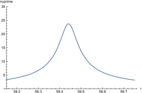
Figure 4: Plot of $d\nu/dr$ near the simulated horizon, for the same parameters used in Fig. 1.

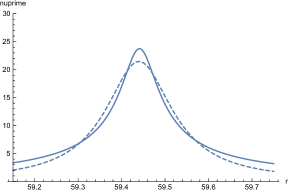
Figure 5: Lorentzian fit of Eq. (18) (dashed line) superimposed on $d\nu/dr$ of Fig. 4 (solid line).

Integrating $d\nu/dr$ gives the solid line plotted in Fig. 6, while integrating the Lorentzian gives an arc tangent function,

$$2.01336\,{\rm ArcTan}[10.65394(r-59.44)]~{}~{}~{},$$ (19)

which, after adding a constant of integration $\nu(59.44)$, is plotted as the dashed line in Fig. 6.

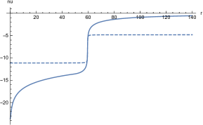
Figure 6: ArcTan resulting from integrating the Lorentzian of Fig. 5 plus constant of integration $\nu(59.44)$ (dashed line) superimposed on $\nu(r)$ (solid line).

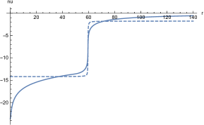
Figure 7: “Eyeball” ArcTan fit (dashed line) superimposed on $\nu(r)$ (solid line).

We see that the behavior of $\nu(r)$ near the simulated horizon is well-modeled by an arc tangent function, which makes a sharp transition from a lower “rail” to an upper “rail”. Rather than integrating the Lorentzian fit to $d\nu/dr$, we can alternatively proceed directly to an “eyeball” fit of an arc tangent to the integrated function $\nu(r)$, again including a constant of integration $\nu(59.44)$,

$$\nu(59.44)+3.95976\,{\rm ArcTan}[9.25686(r-59.44)]~{}~{}~{},$$ (20)

which is plotted as a dashed line in Fig. 7, compared with $\nu(r)$ which is plotted a a solid line. Again, we see that the behavior of $\nu(r)$ near the simulated horizon is well modeled by an arc tangent function. We have focussed on one particular set of parameter values in this section, but the qualitative results given here are typical of a wide range of gravastar parameters.

V Phase diagram for the rescaled equation in the initial pressure – initial mass plane

The kink behavior exhibited in the previous section is typical of a wide range of parameter values. To see this, let us numerically study in more detail the differential equation system of Eq. (14) for $p(r)$ and $m(r)$ . We use the rescaling covariance of Eq. (6) to rescale the initial radius $r_{0}$ to a standard value $r_{0}=50$, chosen to approximate the energy density jump radius $r=48.895$ of Fig. 1, so that a solution close to the one shown there is included in our survey. The remaining parameters of the model are then the initial values $p0\equiv p(r_{0})$ and $m0\equiv m(r_{0})$. We ran the integration of Eqs. (14) for a wide range of initial values $p0$, ranging from $p0=.01$ to $p0=10^{4}$, and for each determined the largest value of $m0$ for which a kink solution resembling Fig. 1 is obtained, as tabulated in Table 1. For larger values of $m0$ than these limiting values, the Mathematica program returns an error message of a “stiff” solution, where in the integrator NDSolve we have used parameters PrecisionGoal and AccuracyGoal of 13 (the maximum attainable on our hardware) and MaxSteps of $10^{10}$. We cannot say whether with more powerful hardware than used in this study the limiting $m0$ value could be pushed higher, so the results we give should be interpreted as least upper bounds on the $m0$ range for which a kink solution is obtained. The results summarized in Table 1 can be plotted as a “phase diagram” in the $p0$–$m0$ plane as shown in Fig. 8, with points in the shaded region giving a kink solution, and points outside the shaded region giving a “stiff” error message. This demonstrates clearly that the horizon-like behavior of Figs. 1 and 2 is not a result of fine tuning of parameter values, but is characteristic of the TOV equation with relativistic matter for a wide range of initial values $p0$, $m0$ at the inner radius $r_{0}$ where the integration is started.

To show the trend of kink shapes as the parameters $p0$ and $m0$ are varied, in Fig. 9 we show plots of $denom$ moving out along the phase space boundary line, with the solid line for $p0=1$, $m0=17.99$ and the dashed line for $p0=1,000$, $m0=-262,000$. In Fig. 10 we give plots of $denom$ moving downwards from the phase space boundary line, with the solid line for $p0=1$, $m0=17.99$, and the dashed line for $p0=1$, $m0=-100$. Finally, Fig. 11 gives similar plots of $denom$ moving downwards from the phase space boundary line, now with the solid line for $p0=1000$, $m0=-262,000$, and the dashed line for $p0=1000$, $m0=-1,000,000$.

Kink shapes can also be characterized by the $r$ value at the center of the dip in $denom$, the minimum attained at this dip, and the width at half maximum $\Delta r$ of the curve for $d\nu/dr$ analogous to Fig. 4, as plotted for each set of parameter values. These are given for $p0=1$ in Table 2, and for $p0=1000$ in Table 3, for a range of values $m0$.

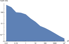
Figure 8: “Phase diagram” in the $p0$, $(25-m0)^{-1}$ plane, where $p0=p(r_{0})$ is the initial pressure and and $m0=m(r_{0})$ is the initial mass. The diagonal boundary corresponds to the largest value of $m0$ for which the Mathematica notebook gives a kink solution; for values of $m0$ corresponding to the region above this boundary the program gives a “stiff” error diagnostic. For points within the shaded region, a kink solution is obtained.

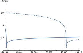
Figure 9: Plots of $denom$ moving out along the phase space boundary line. Solid line is for $p0=1$, $m0=17.99$; dashed line is for $p0=1,000$, $m0=-262,000$.

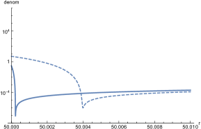
Figure 10: Plots of $denom$ moving downwards from the phase space boundary line. Solid line is for $p0=1$, $m0=17.99$; dashed line is for $p0=1$, $m0=-100$.

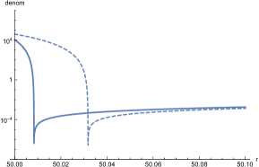
Figure 11: Plots of $denom$ moving downwards from the phase space boundary line. Solid line is for $p0=1000$, $m0=-262,000$; dashed line is for $p0=1000$, $m0=-1,000,000$.

Table 1: Boundary points used to plot Fig. 8

$p0$	m0
0.01	24.9998999
.03162	24.9996004
0.1	24.9899999
.3162	24.9869469
1	24.9651
3.162	24.5310
10	21.366
31.62	-26.75
100	-153
316.2	-806
1000	-4,640
3162	-27,600
10000	-126,000

Table 2: $p0=1$

$m0$	central $r$	depth	width $\Delta r$
$17.99$	$50.00022$	$5.5\cdot 10^{-8}$	$6.17\cdot 10^{-6}$
$17.99-10$	$50.00054$	$1.3\cdot 10^{-7}$	$1.50\cdot 10^{-5}$
$17.99-10^{2}$	50.0034	$8.4\cdot 10^{-7}$	$9.41\cdot 10^{-5}$
$17.99-10^{3}$	50.0322	$7.8\cdot 10^{-6}$	$8.83\cdot 10^{-4}$
$17.99-10^{4}$	50.316	$7.5\cdot 10^{-5}$	$8.48\cdot 10^{-3}$
$17.99-10^{5}$	52.852	$5.3\cdot 10^{-4}$	$6.32\cdot 10^{-2}$

Table 3: $p0=1000$

$m0$	central $r$	depth	width $\Delta r$
-262000	50.0083	$6.5\cdot 10^{-8}$	$7.28\cdot 10^{-6}$
$-262,000-10^{2}$	50.0083	$6.5\cdot 10^{-8}$	$7.29\cdot 10^{-6}$
$-262,000-10^{4}$	50.0087	$6.7\cdot 10^{-8}$	$7.56\cdot 10^{-6}$
$-262,000-10^{6}$	50.0401	$3.1\cdot 10^{-7}$	$3.49\cdot 10^{-5}$
$-262,000-10^{8}$	52.848	$1.7\cdot 10^{-5}$	$2.00\cdot 10^{-3}$
$-262,000-10^{10}$	100.515	$1.9\cdot 10^{-5}$	$4.22\cdot 10^{-3}$

VI Discussion

From the results of the previous sections, we see that the formation of a gravastar simulated horizon is independent of fine details of the interior region phase transition. What is needed is for a sufficiently negative volume integrated energy density $m(r)$ to be present at the inner boundary of the relativistic matter exterior region. This is allowed wald because the energy density $\rho(r)$ can be negative when quantum corrections to the stress-energy tensor are taken into account. Although we have focused our analysis on an exterior region equation of state $\rho(p)=\alpha p$ with $\alpha=3$, a survey with differing values of $\alpha>0$ shows that qualitatively similar behavior is obtained for general $\alpha$, with the sharpness of the kink increasing with $\alpha$. Also, in adler2 it was observed that an exterior equation of state with sufficiently small mass term also leads to formation of a simulated horizon. What seems to be important is that as the pressure $p$ approaches zero, the energy density $\rho(p)$ also rapidly becomes small, so that the bulk of the gravastar mass resides within a compact region of finite radius. Then the Birkhoff uniqueness theorem birk for spherically symmetric solutions of the Einstein equations takes over, and guarantees an exterior metric that is very close to Schwarzschild in form.

VII Acknowledgements

We thank Ahmed ElBanna and Yuqui Li for advice on how to incorporate Mathematica utilities for maximization and minimization into our computations. Dr. ElBanna has placed an annotated version of the Mathematica notebook used for Fig. 8 and Tables 1-3 online at the following URL: https://community.wolfram.com/groups/-/m/t/3022687   .

References

- (1) The Event Horizon Telescope Collaboration, Phys. Rev. Lett. 125, 141104 (2020), arXiv:2010.01055.
- (2) V. Cardoso and P. Pani, Living Rev. Relativ. 22, 4 (2019), arXiv:1904.05363.
- (3) S. L. Adler, Phys. Rev. D 106, 104061 (2022), arXiv:2209.02537.
- (4) S. L. Adler, “ Dynamical gravastars may evade no-go results for exotic compact objects, together with further analytical and numerical results for the dynamical gravastar model”, arXiv:2301.11821.
- (5) Y. Cendes et al., “Ubiquitous Late Radio Emission from Tidal Disruption Events”, arXiv:2308.13595.
- (6) R. M. Wald, “General Relativity”, The University of Chicago Press (1984), p. 410.
- (7) For a modern survey with references, see G. F. R. Ellis and R. Goswami, “Variations on Birkhoff’s theorem”, arXiv:1304.3253.