Output-Sampled
Model Predictive Path Integral Control (o-MPPI)
for Increased Efficiency
Abstract
The success of the model predictive path integral control (MPPI) approach depends on the appropriate selection of the input distribution used for sampling. However, it can be challenging to select inputs that satisfy output constraints in dynamic environments. The main contribution of this paper is to propose an output-sampling-based MPPI (o-MPPI), which improves the ability of samples to satisfy output constraints and thereby increases MPPI efficiency. Comparative simulations and experiments of dynamic autonomous driving of bots around a track are provided to show that the proposed o-MPPI is more efficient and requires substantially (20-times) less number of rollouts and (4-times) smaller prediction horizon when compared with the standard MPPI for similar success rates. The supporting video for the paper can be found at https://youtu.be/snhlZj3l5CE.
I Introduction
Sampling-based approaches such as model predictive path integral control (MPPI) [1] have become popular methods to solve optimization problems due to fast computations possible with graphic processing units and parallelized computing. In such methods, models are used to predict the cost for a series of input rollouts, and the final input selection is a cost-weighted average of the rollouts. An advantage of the sample-based approach is that it is derivative-free, does not require approximation of the system dynamics and cost functions, and allows for non-differentiable cost functions [2].
Successful use of the MPPI algorithm requires proper selections of the mean and the covariance of the input samples. If the selected mean leads to a rollout that enters inside an infeasible region (this could be caused by the poor initialization, system disturbance, or sudden environment changes), then most of the sampled rollouts can result in failure [3]. Although a larger covariance can be used to alleviate failures by increasing exploration [4], it also often requires a larger number of samples and increased computation load, and can lead to undesirable input chattering [1, 5]. Therefore, there is substantial ongoing interest in methods to appropriately select the input samples to improve MPPI performance. However, in general, it is challenging to appropriately select a desirable input mean to meet constraints in the output space, especially in dynamic environments. In general, even when the reference input can be selected as desired outputs to a closed-loop system that satisfies constraints, it does not ensure that the output achieves precision tracking of the desired trajectories.
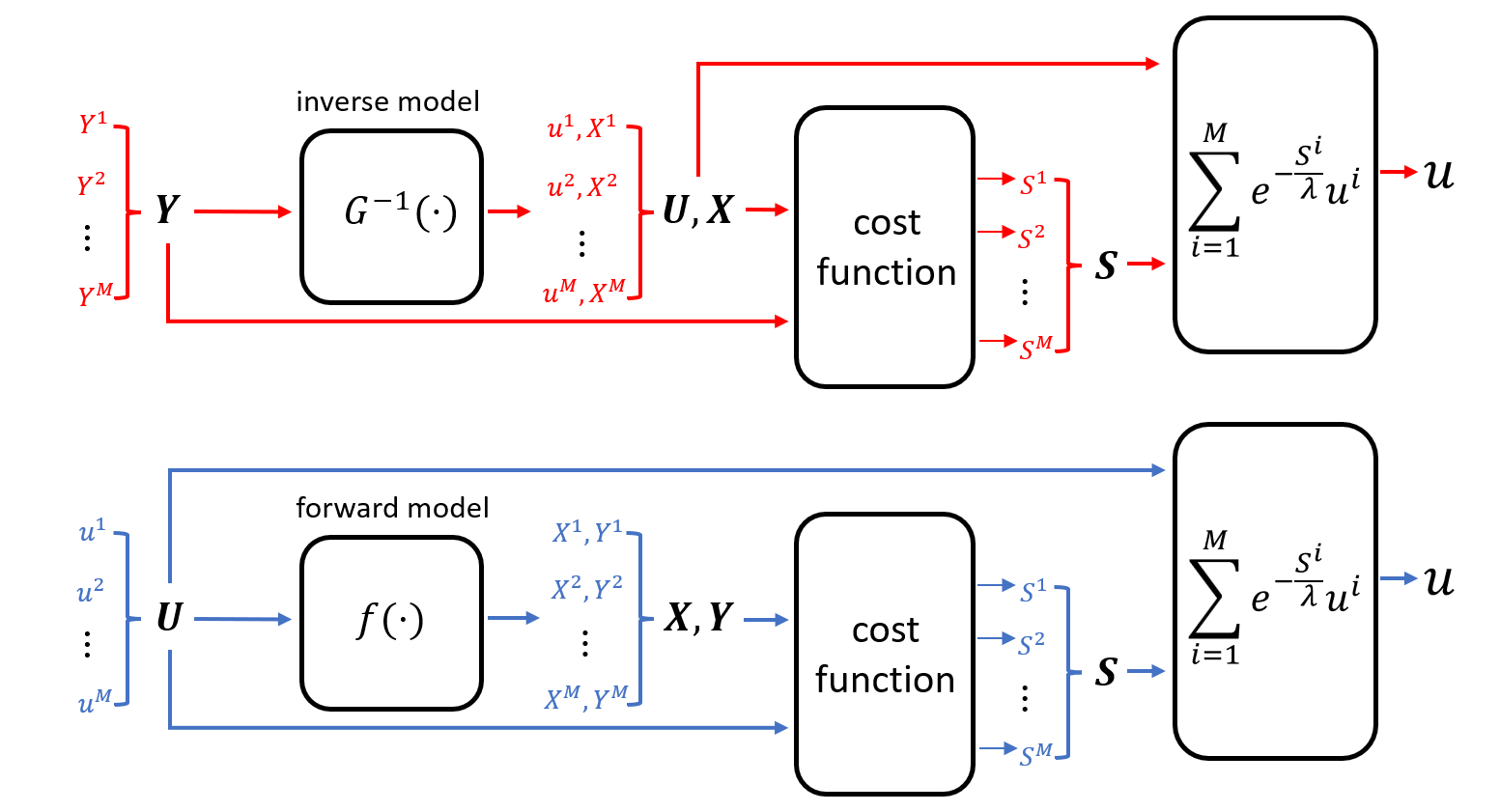
With the goal of increasing rollouts that satisfy output constraints, the current paper proposes the sampling of trajectories directly from the output space. Then, the proposed output-sampling-based MPPI (o-MPPI) approach uses the inverse model to map outputs to inputs rather than the traditional approach in MPPI of using the input-to-output forward model as illustrated in Fig. 1(top). The inputs obtained using the inverse model are then weighted to obtain the optimized control sequence, as in standard MPPI.
The main contributions of the paper are the following.
-
1.
It proposes an output-sampling-based MPPI (o-MPPI) using inverse models, which improves the ability to select rollouts that satisfy typical output constraints. An advantage of output sampling is that it can leverage well-established trajectory planning algorithms in robotics to select output samples and then use inverse models (physics-based or data-based) to find the associated inputs. This is different from selecting inputs and then finding the associated outputs using forward models.
-
2.
Comparative simulations and experiments of autonomous control of bots (TurtleBot3 Burger) in a dynamic autonomous driving around a track, are used to show that the proposed o-MPPI requires substantially (20-times) less number of rollouts and (4-times) smaller prediction horizon when compared with the standard MPPI to achieve a similar success rate.
The paper is organized as follows. Section II discusses the related works. Section III describes the proposed o-MPPI followed by its application to an autonomous driving scenario with moving obstacles in Section IV. Simulation and experimental results are comparatively evaluated and discussed in Section V. Finally, the conclusions and future works are presented in Section VI.
II Related work
II-A MPPI with adjusted trajectory distribution
Several efforts are made to improve the robustness and sample efficiency of standard MPPI by appropriately adjusting the trajectory distribution using different sampling strategies [3, 6, 7, 8]. For example, warm-starts are used [1] to improve MPPI-variants. In [6], covariances are adapted to accommodate different actions for better exploration. In [7], the samples are drawn from a normal and log-normal (NLN) distribution instead of the Gaussian distribution, which can yield improved performance in cluttered environments. In [8], the diagonal covariance matrix is changed into a nondiagonal covariance matrix and updated through the adaptive importance sampling procedure. Recently, constraints were added to the terminal state of the prediction horizon in [3] to adjust the input distribution. In all these works sampling is in the input space followed by the use of forward models to determine the outputs. In contrast, the current work proposes sampling in the output space (since constraints might be more easily satisfied in the output space) and then uses an inverse model to find the corresponding inputs. Once the input-output pairs are found, the proposed o-MPPI is similar to standard MPPI and can use the same cost functions and weighting strategies.
II-B MPPI with output-space-informed mean
The output space has been leveraged in the past to improve the input-sampling efficiency of MPPI. Since a better mean for the input distribution can also help improve MPPI, an appropriately selected output can be used to inform the mean selection used in standard MPPI. For example, in [4], the fast rapid-exploring-tree () algorithm is used to provide guidance about the mean value of the input for improving sampling efficiency in the input space. In [9], trained Conditional Variational Autoencoders that take into account the contextual information are used to better inform the mean values by taking into the control uncertainties. Thus, the above methods utilize output-space information to guide the selection of the mean value for the input sampling. The proposed o-MPPI approach extends this idea and fully samples in the output space and then uses inverse models to find the corresponding input?. It is noted that sampling of the output space has been used in the path-planning community to smooth and potentially optimize feasible trajectories, e.g., [10, 11]. Here, these planned trajectories are inputs to the closed-loop system, and forward models (of the closed-loop system) are used to predict the system response and for optimizing the selected input (final output trajectory) to the closed-loop system. The proposed o-MPPI can be used with any trajectory planning algorithm such as the fast rapid-exploring-tree () [4] – the main difference is that inverse models are used in o-MPPI to find inputs that track the selected output trajectories.
II-C Inverse models
The proposed o-MPPI leverages the strong history in inverse dynamics to find maps from outputs to inputs. For example, physics-based models can be used to analytically find the inverse input [12] in robotics applications. When the physics-based models are not sufficiently precise, the Gaussian process can be used to learn the discrepancy [13]. The entire inverse model can be approximated with deep learning models [14] or Gaussian process models [15]. Additionally, data-enabled models can be used to learn the inverse output-to-input map from input-output data [16]. Thus, the proposed o-MPPI can use a wide range of inverse modeling tools to find the inputs associated with the sampled output trajectories.
III Proposed Framework
The proposed output-sampling-based MPPI (o-MPPI) approach is summarized in Algorithm 1. Essentially, there are four steps (detailed below): (i) selection of the cost function; (ii) sampling in the output space; (iii) inversion to find the associated inputs; and (iv) weighted selection of the input.
As in standard MPPI, a cost function is used to specify the desirability of a specific input-state-output rollout. In particular, consider the optimization
| (1) |
subject to system dynamics
| (2) |
where represents the forward dynamics, maps the state to the output at time step , and the output trajectory is given by . In the above optimization, is the running cost, is the weight matrix of the input energy cost, and the terminal cost is in Eq. (1). Additionally, there are constraints on the output trajectory to lie in an acceptable region, i.e., .
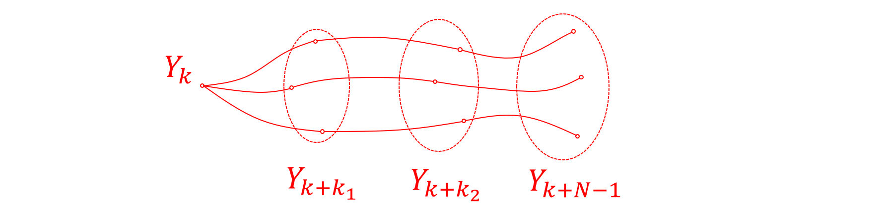
The output sampling can be generated from any trajectory planning method, e.g., parametric ones like spline or bezier curves by specifying the waypoints as in Fig. 2, using optimization methods such as -order constrained path optimization (KOMO) [17], via-point-based Stochastic Trajectory Optimization (VP-STO) [18], or from a data-based planner [19, 20, 21, 22]. For each sampled output, inverse maps are used to find the corresponding input that yields tracking of the output.
The optimized input is obtained as the weighted sum of all the input rollouts as in standard MPPI, i.e.,
| (3) |
where and for are are normalized weights, i.e., .
IV Application of o-MPPI to Experimental setup
The system for evaluating the proposed o-MPPI is set up to mimic a dynamic autonomous driving scenario with moving obstacles.
IV-A System description
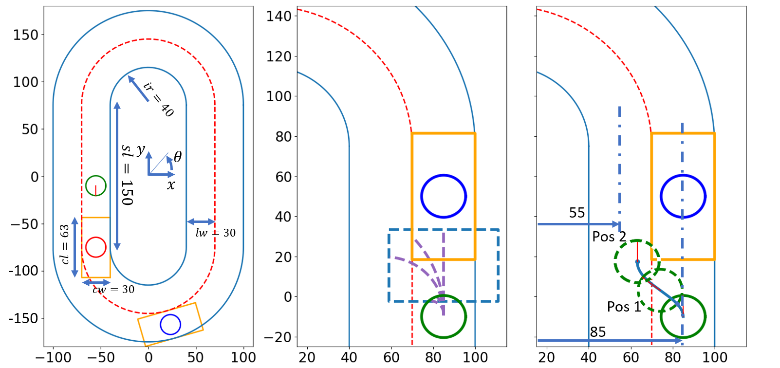
In the experiment, the goal is for a fast bot (green) to move as close as possible to its desired speed of 20 cm/s while maneuvering around slower bots that can be considered as moving obstacles at the same time. The ability for the fast bot to maintain its desired speed and overtake the slower bots, as illustrated in Fig. 3, are used to quantitatively compare the performance of the standard MPPI and the proposed o-MPPI. An example simulation run is shown in the left plot in Fig. 3. The slower bots are moving at constant speeds of 10 cm/s (blue) and 12 cm/s (red). All bots are driving in the counter-clockwise direction in ellipsoidal tracks with dimensions tabulated in Table I and illustrated in Fig. 3, similar to the shape of the track in [23].
| bot turning circle radius (cm) | 10.5 | lane width (cm) | 30 |
|---|---|---|---|
| max vel. (cm/s) | 22 | straight lines (cm) | 150 |
| max angular vel. (rad/s) | 2.8 | inner radius (cm) | 40 |
| collision area width (cm) | 30 | collision area length (cm) | 63 |
IV-B Standard MPPI
IV-B1 Forward model
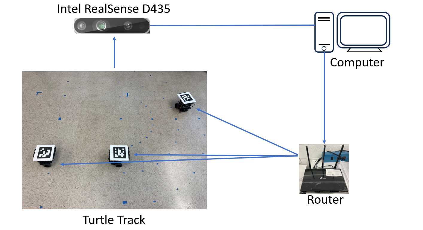
The bot (TurtleBot3 Burger) state at time step is defined as . is the position pair and is the orientation with respect to the Turtle Track coordinates, as in Fig. 3. is the forward velocity and is the angular velocity. The input to the system is where is the desired forward velocity and is the desired angular velocity, and the system output is .
The forward bot dynamics is approximated by the forward Euler discretization ,
| (4) | ||||
| (5) | ||||
| (6) | ||||
| (7) | ||||
| (8) |
where the sampling time is s, if otherwise is a saturation function used to bound with the magnitudes of the speed and angular velocity with and defined in Table I, and the settling-time parameter is estimated from the measured step response.
IV-B2 Cost function selection
The cost function in Eq. (1) is designed to have only the running cost function , with zero input energy cost (=0), similar to the cost functions used in autonomous driving in [23, 24]. The running cost function is designed to have three components, i.e., . The first cost , designed for lane keeping, is the product of the squared values of the bot’s distance to the center lines of the two lanes, as shown in the right plot in Fig. 3. Formally,
| (9) |
where , if is outside of the designed track shown in Fig. 3 and zero otherwise, , and and otherwise. The second cost , designed for driving the bot at a speed close to the desired speed of cm/s, is the squared of the speed difference between the current speed and the desired one,
| (10) |
The third cost , designed to avoid collisions with the slower bots, is set to a large value if is inside the (extended) collision region at time step
| (11) |
where is the turning circle radius, and are the collision region length and width, respectively, as seen in Table I. The computation of the projection distance and are described below
where , and
IV-B3 MPPI algorithm
The standard MPPI [23] algorithm is summarized in Algorithm 2 (blue parts indicate differences from the proposed o-MPPI) with the temperature parameter selected as and the covariance matrix is selected as to enable sufficient exploration. In general, an additional cost can be added to the cost function for input deviation as [23]. However, the hyperparameter is set to zero to promote exploration in the dynamic environment with moving obstacles. The mean of the input distribution in Eq. (3) and the prediction horizon are varied to illustrate their impact on MPPI effectiveness in the results and discussion Section V.
IV-B4 Weighting
Given the trajectory costs for all the rollouts () based on the cost function, the weight associated with each rollout () is computed as , where is the minimum cost of the rollouts and the normalizing factor is .
IV-C o-MPPI
The proposed o-MPPI (see Aglorithm 1) differs from the standard MPPI in the sampling of the output and the use of inverse to find the input – these are described below. The proposed o-MPPI uses the same temperature parameter , cost function and weighting to determine the input as the standard MPPI case in Sections IV-B2 and IV-B3.
IV-C1 Sampling the trajectory rollout
The generic way in Fig. 2 is used to sample the trajectory rollouts in this paper with only two waypoints: the initial output and the final output. Specifically, a rectangle-shape region of interest for the endpoint is determined based on the allowed magnitudes of the inputs and the prediction horizon . Then, the sampled trajectory rollout is generated by fitting cubic splines between the current output and the final output sampled inside the region of interest, as seen in the right plot in Fig. 3. Specifically, the rollout expression (for the output ) is selected as a cubic spine as in [25]
| (12) |
where the coefficients for can be determined from the boundary conditions
where the endpoint orientation is designed to be aligned with the road direction and the endpoint forward speed is the travel distance divided by the prediction horizon , i.e., . The output is generated in a similar manner with the selected final waypoint output .
IV-C2 Inverse model
Given a differentiable output trajectory with and starting state , i.e., , , , , the inverse input can be obtained at time steps with from the forward dynamics in Eq. (7) to (8), as:
| (13) | ||||
where
| (14) | ||||
| (15) | ||||
| (16) |
are the planned speed, angular velocity, and the orientation at time step , respectively. Saturation is not considered when computing the inverse input in Eq. (13). However, if the final optimal input is large (for either o-MPPI or standard MPPI), then it is saturated in the experimental system and bounded in simulations by the saturation function in Eqs. (7)- (8).
V Results and discussion
The ability to avoid and successfully overtake moving obstacles in dynamic environments are comparatively evaluated below for the proposed o-MPPI and the standard MPPI. The evaluation starts with the study of a single dynamic obstacle, which is followed by the case with multiple obstacles.
V-A Case with a single dynamic obstacle
For comparative evaluation with a single obstacle, three MPPI and one o-MPPI cases are simulated with the following conditions.
-
•
Case 1 o-MPPI: The proposed o-MPPI with prediction horizon s.
-
•
Case 2 Small-horizon standard MPPI: Standard MPPI with prediction horizon s, i.e., prediction steps with sampling time period s. The nominal speed is cm/s, i.e., with initial control sequence (in Algorithm 2) ;
-
•
Case 3 Large-horizon standard MPPI: Standard MPPI as in Case 2 except with a larger prediction horizon s and corresponding prediction steps ;
-
•
Case 4 Slow-initial standard MPPI: Standard MPPI as in Case 2 except that the initial speed is lower at cm/s i.e., with initial control sequence (in Algorithm 2) cm/s, rad/s].
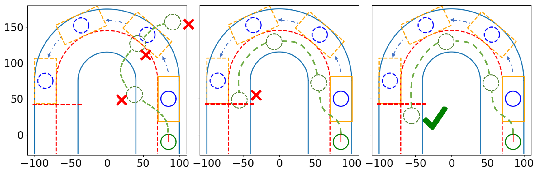
The controlled bot (green in Fig. 5) is said to achieve a successful overtake of a moving obstacle (blue circle in Fig. 5) if: (i) the controlled bot is driving in the counter-clockwise direction all the time, (ii) the controlled bot does not run outside of the track or into the collision regions of the moving obstacle, and (iii) within a specified time, the position of the controlled bot is ahead of the slower constant-speed obstacle. as indicated by the red dashed lines in Fig. 6. For all these cases, the initial position of the moving obstacle is on one corner of the track as shown in Fig. 6 and it has a constant speed of cm/s. The simulation is run till the moving obstacle reaches the other corner of the track as indicated in Fig. 6. The initial position of the controlled bot is behind the moving obstacle at . The initial trajectory rollouts for o-MPPI and standard MPPI for the four different cases are visualized in Fig. 5 for comparative evaluation. Additionally, repeated simulations were run, and the success rates for the four cases with different numbers of rollouts are tabulated in Table II and III.
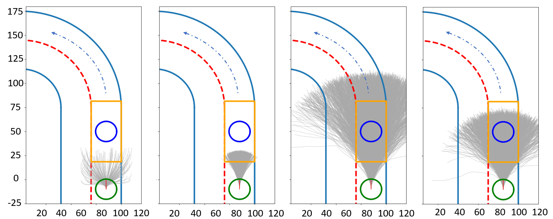
V-A1 Less number of rollouts (efficient exploration)
The proposed o-MPPI method requires -times less number of rollouts compared to the standard MPPI, as seen in Tables III and II, In particular, to achieve success rate of overtaking, the standard MPPI requires rollouts with a prediction horizon s while the o-MPPI method needs rollouts with a prediction horizon s. Thus, the proposed o-MPPI achieves a more efficient exploration compared to standard MPPI.
V-A2 Smaller prediction horizon
The o-MPPI method requires -times smaller prediction horizon compared to the standard MPPI as seen in Table III and II. In particular, to achieve success rate in overtaking, the standard MPPI requires a prediction horizon s while the inversion-based sampling method needs only rollouts with a prediction horizon s.
When the standard MPPI method is restricted to a prediction horizon of s, the controlled bot only achieves around success rate, even with a large number of rollouts . This is because o-MPPI has rollouts that run into the other lane as seen in the second left plot in Fig. 5. In contrast, rollouts of MPPI (rollout number ) with a prediction horizon s) are mostly restricted to within the original lane. Note that the explored area of the standard MPPI increases substantially with a larger prediction horizon of s as seen in Fig. 5.
In this sense, the proposed o-MPPI with a smaller prediction horizon requirement is beneficial since requiring a larger prediction horizon might not be feasible due to sensor-range limitations and it can also lead to increased computational load.
| M | 50 | 100 | 200 |
|---|---|---|---|
| success rate | 100 | 100 | 100 |
V-A3 MPPI performance is susceptible to the slow initial
MPPI performance is susceptible to improper initial input sequences, even with sufficient prediction horizon s and number of rollouts . For Case 4 with slow-initial speed of cm/s example, the controlled bot has difficulty overtaking the moving obstacle since the explored area has less overlap with the overtake regions, as seen in Fig. 5. Therefore, MPPI performance is affected by the initialization strategy and is susceptible to dynamic environments.
. T M succ. rate T M succ. rate Case 2 2.0 50 28 4.0 50 4 2.0 500 28 4.0 500 2 2.0 1000 15 4.0 1000 6 2.0 2000 22 4.0 2000 2 Case 3 8.0 50 49 6.0 50 34 8.0 500 75 6.0 500 52 8.0 1000 100 6.0 1000 89 8.0 2000 100 6.0 2000 97 Case 4 8.0 2000 1
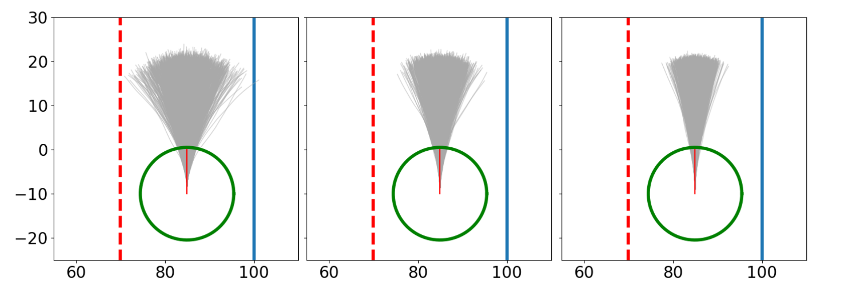
V-A4 Trade-off in sampling time selection with MPPI
Generally, a higher sampling rate for control is beneficial since this can lead to more precision. However, a higher rate of control also results in a higher dimensional search space for input sampling, which requires more samples to be drawn for sufficient exploration, as illustrated in Fig. 7. Less exploration can also result in less success since the best rollout may not be explored when the environment changes too fast or uncertainties are large. In contrast, since the o-MPPI trajectory rollouts are sampled from the potential set of waypoints in the output space that only depends on the prediction horizon , the control sampling rate does not affect the explored region.
V-B Case with multiple dynamic obstacles
For comparative evaluation with multiple obstacles, two moving obstacles are considered as in the left plot of Fig. 3. The cost function is kept the same as in the previous Section V-A with a single dynamic obstacle.
The first obstacle has a constant speed of cm/s (red circle) and tracks the inner lane with initial position and the second obstacle has speed cm/s (blue circle) and tracks the outer lane with initial position . The initial position of the controlled bot (green) is behind the first moving obstacle and has the initial condition Comparative simulation and experiments of o-MPPI and standard MPPI were performed with settings as in Case 1 (o-MPPI) and Case 3 (Larger-horizon standard MPPI) proposed in Section V-A.
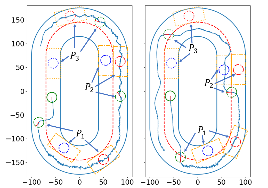
V-B1 Comparison of two obstacle avoidance
Only the o-MPPI-controlled bot managed to successfully maneuver around both moving obstacles after slowing down because both lanes were blocked by the two slower constant-speed bots as seen in the trace plots in Fig. 8. First, the o-MPPI-controlled bot switched to the inner lane since the inner-lane, constant-speed bot has a relatively faster speed at cm/s compared to the outer-lane, constant-speed bot moving at cm/s and second then the o-MPPI-controlled bot switched back to the outer lane once there is sufficient room to drive at a faster speed that is closer to the desired speed cm/s. In contrast, the standard MPPI-controlled bot got stuck behind the constant-speed bot, as seen from the trace in the upper region of the track in Fig. 8. As shown with Case 4 (slow-initial standard MPPI), with a smaller speed the nominal mean of the MPPI input distribution become smaller, and can lead to lower success rate for overtaking. It is noted that both the o-MPPI-controlled bot and the MPPI-controlled bot were able to successfully maneuver around a single obstacle when the controlled bot is moving at a higher speed as seen in the accompanying video at https://youtu.be/snhlZj3l5CE.
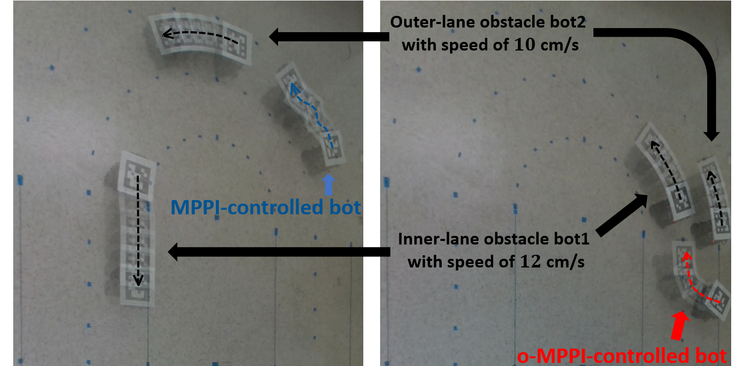
V-B2 Oscillatory driving versus overtaking
Comparison of overlays of the experimental snapshots in Fig. 9 (left) shows that the MPPI-controlled bot can not only get stuck behind the slower moving obstacle bot (with speed cm/s in the outer lane), but it also tends to have oscillatory driving behavior. This is because the oscillatory motion allows the bot to achieve a relatively faster speed closer to its desired speed in the cost function component in Eq. (10). In contrast, overlays of the o-MPPI-controlled bot in Fig. 9 (right) show that it is able to maintain higher speed by successfully switching to the inner lane since the obstacle bot in the inner lane in the front has a higher speed cm/s compared to the bot in the outer lane with speed cm/s.
VI Conclusion and Future works
This paper proposed an output-sampling-based model predictive path integral control (o-MPPI) to improve the efficiency of standard MPPI. An advantage of the proposed output sampling is that it can leverage the substantial work on trajectory planning in robotics to meet constraints that are often posed in the output space, which in turn improves the efficiency of MPPI. Instead of forward models that map from input to output as in standard MPPI, the proposed o-MPPI uses inverse models to map from the sampled output to inputs. The improved efficiency of the o-MPPI was seen in both the simulation and the experimental results — o-MPPI required less number of rollouts and a shorter prediction horizon, compared to the standard MPPI. Future works will explore the use of other trajectory-planning methods for output sampling with o-MPPI, as well as the use of data-enabled deep-learning and Gaussian process models for the inverse map. A blending of the input sampling and output sampling can also be considered depending on the type of constraints.
References
- [1] Grady Williams, Andrew Aldrich, and Evangelos A Theodorou. Model predictive path integral control: From theory to parallel computation. Journal of Guidance, Control, and Dynamics, 40(2):344–357, 2017.
- [2] Ihab S Mohamed, Guillaume Allibert, and Philippe Martinet. Model predictive path integral control framework for partially observable navigation: A quadrotor case study. In 2020 16th International Conference on Control, Automation, Robotics and Vision (ICARCV), pages 196–203. IEEE, 2020.
- [3] Ji Yin, Zhiyuan Zhang, Evangelos Theodorou, and Panagiotis Tsiotras. Trajectory distribution control for model predictive path integral control using covariance steering. In 2022 International Conference on Robotics and Automation (ICRA), pages 1478–1484. IEEE, 2022.
- [4] Chuyuan Tao, Hunmin Kim, and Naira Hovakimyan. RRT-guided model predictive path integral method. arXiv preprint arXiv:2301.13143, 2023.
- [5] Taekyung Kim, Gyuhyun Park, Kiho Kwak, Jihwan Bae, and Wonsuk Lee. Smooth model predictive path integral control without smoothing. IEEE Robotics and Automation Letters, 7(4):10406–10413, 2022.
- [6] Mohak Bhardwaj, Balakumar Sundaralingam, Arsalan Mousavian, Nathan D Ratliff, Dieter Fox, Fabio Ramos, and Byron Boots. Storm: An integrated framework for fast joint-space model-predictive control for reactive manipulation. In Conference on Robot Learning, pages 750–759. PMLR, 2022.
- [7] Ihab S Mohamed, Kai Yin, and Lantao Liu. Autonomous navigation of agvs in unknown cluttered environments: log-mppi control strategy. IEEE Robotics and Automation Letters, 7(4):10240–10247, 2022.
- [8] Dylan M Asmar, Ransalu Senanayake, Shawn Manuel, and Mykel J Kochenderfer. Model predictive optimized path integral strategies. In 2023 IEEE International Conference on Robotics and Automation (ICRA), pages 3182–3188. IEEE, 2023.
- [9] Raphael Kusumoto, Luigi Palmieri, Markus Spies, Akos Csiszar, and Kai O Arras. Informed information theoretic model predictive control. In 2019 International Conference on Robotics and Automation (ICRA), pages 2047–2053. IEEE, 2019.
- [10] Mrinal Kalakrishnan, Sachin Chitta, Evangelos Theodorou, Peter Pastor, and Stefan Schaal. Stomp: Stochastic trajectory optimization for motion planning. In 2011 IEEE International Conference on Robotics and Automation (ICRA), pages 4569–4574. IEEE, 2011.
- [11] Liang Ma, Jianru Xue, Kuniaki Kawabata, Jihua Zhu, Chao Ma, and Nanning Zheng. Efficient sampling-based motion planning for on-road autonomous driving. IEEE Transactions on Intelligent Transportation Systems, 16(4):1961–1976, 2015.
- [12] Santosh Devasia, Degang Chen, and Brad Paden. Nonlinear inversion-based output tracking. IEEE Transactions on Automatic Control, 41(7):930–942, 1996.
- [13] Franziska Meier, Daniel Kappler, Nathan Ratliff, and Stefan Schaal. Towards robust online inverse dynamics learning. In 2016 IEEE/RSJ International Conference on Intelligent Robots and Systems (IROS), pages 4034–4039. IEEE, 2016.
- [14] Athanasios S Polydoros, Lazaros Nalpantidis, and Volker Krüger. Real-time deep learning of robotic manipulator inverse dynamics. In 2015 IEEE/RSJ International Conference on Intelligent Robots and Systems (IROS), pages 3442–3448. IEEE, 2015.
- [15] Diego Romeres, Mattia Zorzi, Raffaello Camoriano, Silvio Traversaro, and Alessandro Chiuso. Derivative-free online learning of inverse dynamics models. IEEE Transactions on Control Systems Technology, 28(3):816–830, 2019.
- [16] Leon Liangwu Yan and Santosh Devasia. Precision data-enabled koopman-type inverse operators for linear systems. IFAC-PapersOnLine, 55(37):181–186, 2022.
- [17] Marc Toussaint. A tutorial on newton methods for constrained trajectory optimization and relations to slam, gaussian process smoothing, optimal control, and probabilistic inference. Geometric and numerical foundations of movements, pages 361–392, 2017.
- [18] Julius Jankowski, Lara Brudermüller, Nick Hawes, and Sylvain Calinon. Vp-sto: Via-point-based stochastic trajectory optimization for reactive robot behavior. In 2023 IEEE International Conference on Robotics and Automation (ICRA), pages 10125–10131. IEEE, 2023.
- [19] Oktay Arslan and Panagiotis Tsiotras. Machine learning guided exploration for sampling-based motion planning algorithms. In 2015 IEEE/RSJ International Conference on Intelligent Robots and Systems (IROS), pages 2646–2652. IEEE, 2015.
- [20] Ahmed H Qureshi, Anthony Simeonov, Mayur J Bency, and Michael C Yip. Motion planning networks. In 2019 International Conference on Robotics and Automation (ICRA), pages 2118–2124. IEEE, 2019.
- [21] Jacob J Johnson, Linjun Li, Fei Liu, Ahmed H Qureshi, and Michael C Yip. Dynamically constrained motion planning networks for non-holonomic robots. In 2020 IEEE/RSJ International Conference on Intelligent Robots and Systems (IROS), pages 6937–6943. IEEE, 2020.
- [22] Jiankun Wang, Wenzheng Chi, Chenming Li, Chaoqun Wang, and Max Q-H Meng. Neural RRT*: Learning-based optimal path planning. IEEE Transactions on Automation Science and Engineering, 17(4):1748–1758, 2020.
- [23] Grady Williams, Paul Drews, Brian Goldfain, James M Rehg, and Evangelos A Theodorou. Information-theoretic model predictive control: Theory and applications to autonomous driving. IEEE Transactions on Robotics, 34(6):1603–1622, 2018.
- [24] Ji Yin, Zhiyuan Zhang, and Panagiotis Tsiotras. Risk-aware model predictive path integral control using conditional value-at-risk. In 2023 IEEE International Conference on Robotics and Automation (ICRA), pages 7937–7943. IEEE, 2023.
- [25] Zhimin Zhang, John Tomlinson, and Clyde Martin. Splines and linear control theory. Acta Applicandae Mathematica, 49:1–34, 1997.