Combining Strong Convergence, Values Fast Convergence and Vanishing of Gradients for a Proximal Point Algorithm Using Tikhonov Regularization in a Hilbert Space

Abstract.

In a real Hilbert space $\mathcal{H}$. Given any function $f$ convex differentiable whose solution set ${\rm argmin}\kern 1.19995pt_{\mathcal{H}}\,f$ is nonempty, by considering the Proximal Algorithm $x_{k+1}=\text{prox}_{\beta_{k}f}(dx_{k})$, where $0<d<1$ and $(\beta_{k})$ is nondecreasing function, and by assuming some assumptions on $(\beta_{k})$, we will show that the value of the objective function in the sequence generated by our algorithm converges in order $\mathcal{O}\left(\frac{1}{\beta_{k}}\right)$ to the global minimum of the objective function, and that the generated sequence converges strongly to the minimum norm element of ${\rm argmin}\kern 1.19995pt_{\mathcal{H}}\,f$, we also obtain a convergence rate of gradient toward zero. Afterwards, we extend these results to non-smooth convex functions with extended real values.

Akram Chahid Bagy${}^{{\href mailto:akram.bagy@gmail.com}}$, Zaki Chbani${}^{{\href mailto:chbaniz@uca.ac.ma}}$ and Hassan Riahi${}^{{\href mailto:h-riahi@uca.ac.ma}}$

Faculty of Sciences Semlalia, Mathematics, Cadi Ayyad university

40000 Marrakech, Morroco

1. Introduction

In a Hilbert setting $\mathcal{H}$, we denote by $\langle\cdot,\cdot\rangle$ and $\|\cdot\|$ the associate inner product and norm respectively. Let $f:\,\mathcal{H}\rightarrow]-\infty,+\infty]$ be a proper lower semicontinuous convex function. Consider the following optimization problem

$$(\mathcal{P}) \min\left\{f(x):\,x\in\mathcal{H}\right\},$$

whose global solution set $S:={\rm argmin}\kern 1.19995pt_{\mathcal{H}}f$ is assume to be nonempty.

The goal of this paper is to construct a suitable sequence $(x_{k})$ in order to jointly obtain the fast rate of convergence for the objective function $f(x_{k})$ to the optimal value $f^{\star}=\min_{\mathcal{H}}f$, the fast rate norm convergence to zero of a selected gradient in the subdifferential $\partial f(x_{k})$, and also the strong convergence of the iterates $x_{k}$ to $x^{\star}$ the element of minimum norm of $S$. As a guide in our study, we first rely on the asymptotic behaviour of trajectories of a suitable continuous dynamical system. So, let’s first recall some classic results concerning the algorithms associated with the continuous steepest descent. Given $\lambda>0$, the gradient descent method

$$x_{k+1}=x_{k}-\lambda\nabla f(x_{k})$$

and the proximal point method

$$x_{k+1}=\text{prox}_{\lambda f}(x_{k})=\mbox{\rm{argmin}}_{\xi\in\mathcal{H}}\left(\lambda f(\xi)+\frac{1}{2}\|x-\xi\|^{2}\right)$$

are the basic blocks for algorithms in convex optimization. By strong convexity of $\lambda f(\cdot)+\frac{1}{2}\|x-\cdot\|^{2}$, its minimizer always exists and is unique, so that the proximal operator $\text{prox}_{\lambda f}(\cdot)$ is well defined on the hole space $\mathcal{H}$.

By interpreting $\lambda$ as a fixed time step, these two algorithms can be respectively obtained as either the forward (explicit: $\frac{x_{k+1}-x_{k}}{\lambda}+{\nabla}f(x_{k})=0$) or the backward (implicit: $\frac{x_{k+1}-x_{k}}{\lambda}+{\nabla}f(x_{k+1})=0$) discretization of the continuous system

(1) $$\dot{x}(t)+\nabla f(x(t))=0.$$

This gradient method goes back to Cauchy (1847), while the proximal algorithm was first introduced by Martinet [25] (1970), and then developed by Rockafellar [36] who extended it to solve monotone inclusions. One can consult [13], [31], [32], [33], [35], for a recent account on the proximal methods, that play a central role in nonsmooth optimization as a basic block of many splitting algorithms.

Recently, research axes have focused on coupling first-order time-gradient systems with a Tikhonov approximation whose coefficient tends asymptotically to zero. Let us recall that by solving a general ill posed problem $b=Bx$ in the sense of Hadamard, Tikhonov proposed the new method which he called a method of ”regularization”, see [40, 41]. This method, which has been developed in [27, 42] and references therein, consists first in solving the well-posed problem $b=Bx_{\epsilon}+\epsilon x_{\epsilon}$, and then in converging $x_{\epsilon}$ towards a selected point $\bar{x}$ (as $\epsilon\rightarrow 0$) which verifies $B\bar{x}=b$.

The minimization of the function $\varphi_{t}(x):=f(x)+\dfrac{c}{2\beta(t)}\left\lVert x\right\rVert^{2}$, where $c$ is a positive real number and $\beta(t)$ goes to $+\infty$ as $t\rightarrow+\infty$, can be seen as a penalization of the problem of minimizing the objective function $\frac{1}{2}\|\cdot\|^{2}$ under the constraint $x\in\text{argmin}f$. This is also a two level hierarchical minimization problem, see [18, 12, 11, 19].
Knowing that $\frac{c}{2}\left\lVert\cdot\right\rVert^{2}+\beta(t)f(\cdot)$ cross towards $\frac{c}{2}\left\lVert\cdot\right\rVert^{2}+\iota_{\text{argmin}f}(\cdot)$ as $t\rightarrow+\infty$ if $\iota_{C}$ is the indicator function of the set $C$, i.e., $\iota_{C}(x)=0$ for $x\in C$, and $+\infty$ outwards. This monotone convergence is proved as a variational convergence and then as $t\rightarrow+\infty$ (see [1, Theorems 3.20, 3.66]) the corresponding weak$\times$strong or strong $\times$weak graph convergence of the associated subdifferential operators: $\nabla(\frac{c}{2}\left\lVert\cdot\right\rVert^{2}+\beta(t)f){\displaystyle\longrightarrow^{G}}\partial(\frac{c}{2}\left\lVert\cdot\right\rVert^{2}+\iota_{\text{argmin}f})$, the convex subdifferential associated to the proper convex lower semicontinuous function $\frac{c}{2}\left\lVert\cdot\right\rVert^{2}+\iota_{\text{argmin}f}(\cdot)$. As $t\rightarrow+\infty$, suppose that the unique minimizer $z_{t}$ of $\frac{c}{2}\left\lVert\cdot\right\rVert^{2}+\beta(t)f$ weakly converges to some $\bar{z}$, then $(z_{t},0)$ weak$\times$strong converges to $(\bar{z},0)$ in the graph of $\partial(\frac{c}{2}\left\lVert\cdot\right\rVert^{2}+\iota_{\text{argmin}f})$; this can be explained as

$$0\in\partial\left(\dfrac{c}{2}\left\lVert\cdot\right\rVert^{2}+\iota_{\text{argmin}f}\right)(\bar{z})=c\bar{z}+\partial(\iota_{\text{argmin}f})(\bar{z}).$$

The final equality is due to continuity of the convex function $\frac{c}{2}\left\lVert\cdot\right\rVert^{2}$ at some point in the nonempty set ${\text{argmin}f}$, which is the effective domaine of the convex lower semicontinuous function $\iota_{\text{argmin}f}$.

As asymptotical behaviour, for $t\rightarrow+\infty$, this can be explained as the steepest descent dynamical system

(2) $$0\in\dot{x}(t)+\partial\left(\dfrac{c}{2}\left\lVert\cdot\right\rVert^{2}+\beta(t)f\right)(x(t))=\dot{x}(t)+cx(t)+\beta(t)\partial f(x(t)).$$

An abundant literature has been devoted to the asymptotic hierarchical minimization property which results from the introduction of a vanishing viscosity term (in our context the Tikhonov approximation) in gradient-like dynamics. For first-order gradient systems and subdifferential inclusions, see [2, 10]. In [10], Attouch and Cominetti coupled the dynamic steepest descent method and a Tikhonov regularization term

$$\dot{x}(t)+\partial f(x(t))+\epsilon(t)x(t)\ni 0.$$

The striking point of their analysis is the strong convergence of the trajectory $x(t)$ when the regularization parameter $\epsilon(t)$ tends to zero with a sufficiently slow rate of convergence $\epsilon\not\in L^{1}(\mathbb{R}_{+},\mathbb{R})$. Then the strong limit is the minimum norm element of $\text{agrmin }f$. However, if $\epsilon(t)=0$ we can only expect a weak convergence of the induced trajectory $x(t)$. Attouch and Czarnecki in [12, Theorem 3.1] studied the asymptotic behaviour, as time variable $t$ goes to $+\infty$, of a general nonautonomous first order dynamical system

$$0\in\dot{x}(t)+\partial\varphi(x(t))+\beta(t)\partial f(x(t)),$$

and proved weak convergence of $x(t)$ to some $\bar{x}$ in $\text{argmin}\varphi$ on ${\text{argmin}f}$ that satisfies $0\in\partial(\varphi+\iota_{\text{argmin}f})(\bar{x})$. This can be translated for $\varphi=\frac{1}{2}\|\cdot\|^{2}$ to $\bar{x}$ is the minimal norm solution of $(\mathcal{P})$. This can be considered as a combination of two techniques: the time scaling of a damped inertial gradient system (see [7, 8, 4]), and the Tikhonov regularization of such systems (see [9, 3] and related references).

Our approach in this paper is first to derive, via Lyapunov analysis, convergence results ensuring fast convergence of values, fast convergence of gradients towards zero and strong convergence towards the minimum norm element of $S=\text{argmin}_{\mathcal{H}}f$, of solution of the Cauchy type dynamical system

(3) $$\dot{x}(t)+\beta(t){\nabla}f(x(t))+cx(t)=0.$$

This makes it possible to emerge simpler and less technical proofs and thus to better schematize the proof of the results associated with the algorithms generated by the proposed discretizations.

So, to attain a solution of the problem $(\mathcal{P})$ for nonsmooth convex function $f$, we consider the following implicit discretization of the set-valued system $0\in\dot{x}(t)+\beta(t)\partial f(x(t))+cx(t),$ with $\beta(k)=\frac{\beta_{k}}{d}$ and $c=\frac{1-d}{d}\in]0,1[$:

(4) $$x_{k+1}-x_{k}+\dfrac{\beta_{k}}{d}\partial f(x_{k+1})+\dfrac{1-d}{d}x_{k+1}\ni 0.$$

Recall that the proximal operator can be formulated as follows $\text{prox}_{\beta f}(x):=\left(I+\beta\partial f\right)^{-1}(x)$, then iteration (4) can be reformulated as the proximal algorithm:

(5) $$x_{k+1}=\text{prox}_{\beta_{k}f}(dx_{k}).$$

Thus, we adhere to establish similar proposals as fast convergence of values and gradients towards zero and strong convergence of the proximal algorithm (5) to $x^{*}$ under suitable conditions on the sequence $(\beta_{k}).$

The organization of the rest of the paper is as follows. In second section we recall basic facts concerning Tikhonov approximation. We also show the main result of this work concerning the strong convergence property of algorithm (5). In section 3, we apply these results to the two particular cases of the sequence $(\beta_{k})$. Finally, the last section is devoted to the extension of these results to nonsmooth convex functions.

2. Convergence rates for continuous case

Return to the differential equation (3) :

$$\dot{x}(t)+\beta(t){\nabla}f(x(t))+cx(t)=0.$$

We suppose the following conditions:

$$(\mathbf{H}_{f}) \left\{\begin{array}[]{lll}(i)&&f\textit{ is convex and differentiable on }\mathcal{H},\\ \\ (ii)&&S:={\rm argmin}\kern 1.19995pt\,f\neq\emptyset\,,\\ \\ (iii)&&\nabla f\textit{ Lipschitz continuous on bounded subsets of }\mathcal{H},\end{array}\right.$$

and, there exists $\mu>0$ such that, for $t>t_{0}$

$$(\mathbf{H}_{\beta}) \;\left\{\begin{array}[]{lll}(i)&&\beta(t)\text{ is a positive,}\;\mathcal{C}^{2}\,\text{ function with }\dot{\beta}(t)\neq 0,\\ \\ (ii)&&\max\left(\dfrac{\dot{\beta}(t)}{\beta(t)}\;,\;1\right)\leq c-\mu,\\ (iii)&&{\underset{t\rightarrow+\infty}{\limsup}\,\dfrac{1+\dfrac{\dot{\beta}(t)}{\beta(t)}}{\mu+\dfrac{\ddot{\beta}(t)}{{\dot{\beta}}(t)}-\dfrac{\dot{\beta}(t)}{\beta(t)}}<+\infty.}\end{array}\right.\hskip 85.35826pt$$

Let us denote by $x^{*}$ the minimum norm element of $S$, and introduce the energy function $E(t)$ that is defined on $[t_{0},+\infty[$ by

(6) $$E(t):=\beta(t)\left(\varphi_{t}(x(t))-\varphi_{t}(y(t))\right)+\dfrac{c}{2}\|x(t)-y(t)\|^{2}$$

where $x(t)$ is a solution of (3), $y(t)={\rm argmin}\kern 1.19995pt_{\mathcal{H}}{\varphi}_{t}$ and $\varphi_{t}(x):=f(x)+\dfrac{c}{2\beta(t)}\|x\|^{2}.$
We remark that (3) becomes

(7) $$\dot{x}(t)+\beta(t){\nabla}\varphi_{t}(x(t))=0.$$

and, under the initial condition $x(t_{0})=x_{0}\in\mathcal{H}$, it admits a unique solution.

Theorem 2.1.

Let $f:\mathcal{H}\rightarrow\mathbb{R}$ be a convex function satisfying condition $(\mathbf{H}_{f})$ and $x(.):[t_{0},+\infty[\rightarrow\mathcal{H}$ be a solution of the system (3).
If $\beta(t)$ satisfies $(\mathbf{H}_{\beta})$, then $x(t)$ strongly converges to $x^{*}$, and there exists $t_{1}\geq t_{0}$ such that, for $t\geq t_{1}$

(8) $$f(x(t))-\min_{\mathcal{H}}f=\mathcal{O}\left(\dfrac{1}{\beta(t)}\right);$$

(9) $$\|x(t)-y(t)\|^{2}=\mathcal{O}\left(\frac{1}{e^{\mu t}}+\dfrac{\dot{\beta}(t)}{\beta(t)}\right);$$

(10) $$\left\lVert\nabla f(x(t))\right\rVert^{2}=\mathcal{O}\left(\dfrac{1}{\beta^{(}t)}\right).$$

Proof.

We have defined $E(t)$ in (6) by $E(t)=A(t)+B(t)$ where

$$A(t)=\beta(t)\left(\varphi_{t}(x(t))-\varphi_{t}(y(t))\right)\text{and }B(t)=\dfrac{c}{2}\left\lVert x(t)-y(t)\right\rVert^{2}.$$

So, we need to fit a first order differential inequality on $E(t)$ in order to be able to get the desired upper bound

(11) $$E(t)\leq\frac{E(t_{1})\gamma(t_{1})}{\gamma(t)}+\frac{(1+M)\|x^{*}\|^{2}}{2\gamma(t)}\int_{t_{1}}^{t}\dfrac{c(s)\dot{\beta}(s)}{\beta(s)}\gamma(s)ds.$$

To calculate the derivative of the functions $A(t)$ and $B(t)$, we remark that the mapping $t\mapsto y(t)$ is absolutely continuous (indeed locally Lipschitz), see [17, section VIII.2]. We conclude that $y(t)$ is almost everywhere differentiable on $[t_{0},+\infty[$, and then using differentiability of $f$, we also deduce almost everywhere differentiability of $A(t)$ and $B(t)$ on the same intervalle. Thus, we have

$$\dot{A}(t)=\dot{\beta}(t)\left(\varphi_{t}(x(t))-\varphi_{t}(y(t))\right)+\beta(t)\left(\dfrac{d}{dt}\left(\varphi_{t}(x(t))\right)-\dfrac{d}{dt}\left(\varphi_{t}(y(t))\right)\right).$$

Using the derivative calculation and (7), we remark that

$$\begin{array}[]{lll}\dfrac{d}{dt}\left(\varphi_{t}(x(t))\right)&=&\dfrac{d}{dt}\left(f(x(t))+\dfrac{c}{2\beta(t)}\left\lVert x(t)\right\rVert^{2}\right)\\ \\ &=&\large\langle\dot{x}(t)\,,\,\nabla f(x(t))\large\rangle-\dfrac{c\dot{\beta}(t)}{2\beta^{2}(t)}\left\lVert x(t)\right\rVert^{2}+\dfrac{c}{\beta(t)}\large\langle\dot{x}(t)\,,\,x(t)\large\rangle\\ \\ &=&\large\langle\dot{x}(t)\,,\,\nabla f(x(t))+\dfrac{c}{\beta(t)}x(t)\large\rangle-\dfrac{c\dot{\beta}(t)}{2\beta^{2}(t)}\left\lVert x(t)\right\rVert^{2}\\ \\ &=&\large\langle\dot{x}(t)\,,\,\nabla\varphi_{t}(x(t))\large\rangle-\dfrac{c\dot{\beta}(t)}{2\beta^{2}(t)}\left\lVert x(t)\right\rVert^{2}\\ &=&-\beta(t)\left\|\nabla\varphi_{t}(x(t))\right\|^{2}-\dfrac{c\dot{\beta}(t)}{2\beta^{2}(t)}\left\lVert x(t)\right\rVert^{2}\end{array}$$

On the other hand, according to [3, Lemma 2(i)], we have

$$\dfrac{d}{dt}\left(\varphi_{t}(y(t))\right)=\dfrac{-c\dot{\beta}(t)}{2\beta^{2}(t)}\left\lVert y(t)\right\rVert^{2}.$$

Thus

(12) $$\dot{A}(t)=\dot{\beta}(t)\left(\varphi_{t}(x(t))-\varphi_{t}(y(t))\right)-\beta^{2}(t)\left[\left\|\nabla\varphi_{t}(x(t))\right\|^{2}+\dfrac{c\dot{\beta}(t)}{2\beta^{3}(t)}\left(\left\lVert x(t)\right\rVert^{2}-\left\lVert y(t)\right\rVert^{2}\right)\right].$$

We also have

$$\begin{array}[]{lll}\dot{B}(t)&=&c\large\langle x(t)-y(t)\,,\,\dot{x}(t)-\dot{y}(t)\large\rangle\\ &=&-c\large\langle x(t)-y(t)\,,\,\beta(t)\nabla\varphi_{t}(x(t))+\dot{y}(t)\large\rangle.\end{array}$$

Noting that for every $u,v\in\mathcal{H},\,\lambda>0$, $\langle u,v\rangle\leq\frac{\lambda}{2}\|u\|^{2}+\frac{1}{2\lambda}\|v\|^{2}$, we get

$$-c\large\langle x(t)-y(t)\,,\,\dot{y}(t)\large\rangle\leq\dfrac{c}{2}\left(\left\lVert x(t)-y(t)\right\rVert^{2}+\left\lVert\dot{y}(t)\right\rVert^{2}\right).$$

Using [3, Lemma 2(ii)], we obtain $\left\lVert\dot{y}(t)\right\rVert\leq\dfrac{\dot{\beta}(t)}{\beta(t)}\left\lVert y(t)\right\rVert\leq\dfrac{\dot{\beta}(t)}{\beta(t)}\left\lVert x^{*}\right\rVert$; we conclude

(13) $$-c\large\langle x(t)-y(t)\,,\,\dot{y}(t)\large\rangle\leq\dfrac{c}{2}\left(\left\lVert x(t)-y(t)\right\rVert^{2}+\dfrac{\dot{\beta}^{2}(t)}{\beta^{2}(t)}\left\lVert x^{*}\right\rVert^{2}\right).$$

Observe that for $c>0$ the function $\varphi_{t}$ is $\frac{c}{\beta(t)}$-strongly convex, then we have

$$-c\beta(t)\large\langle\nabla\varphi_{t}(x(t))\,,\,x(t)-y(t)\large\rangle\leq-c\beta(t)\left(\varphi_{t}(x(t))-\varphi_{t}\left(y(t)\right)\right)-\dfrac{c^{2}}{2}\left\lVert x(t)-y(t)\right\rVert^{2}.$$

Thus

(14) $$\begin{array}[]{lll}\dot{B}(t)&\leq&\dfrac{c}{2}\left(\left\lVert x(t)-y(t)\right\rVert^{2}+\dfrac{\dot{\beta}^{2}(t)}{\beta^{2}(t)}\left\lVert x^{*}\right\rVert^{2}\right)\\ &&-c\beta(t)\left(\varphi_{t}(x(t))-\varphi_{t}\left(y(t)\right)\right)-\dfrac{c^{2}}{2}\left\lVert x(t)-y(t)\right\rVert^{2}\\ &=&\dfrac{(1-c)c}{2}\left\lVert x(t)-y(t)\right\rVert^{2}+\dfrac{c\dot{\beta}^{2}(t)}{2\beta^{2}(t)}\left\lVert x^{*}\right\rVert^{2}-c\beta(t)\left(\varphi_{t}(x(t))-\varphi_{t}\left(y(t)\right)\right).\end{array}$$

Due to the inequalities (12) and (14), we get

(15) $$\begin{array}[]{lll}\dot{E}(t)&\leq&\dot{\beta}(t)\left(\varphi_{t}(x(t))-\varphi_{t}(y(t))\right)-\beta^{2}(t)\left[\left\|\nabla\varphi_{t}(x(t))\right\|^{2}+\dfrac{c\dot{\beta}(t)}{2\beta^{3}(t)}\left(\left\lVert x(t)\right\rVert^{2}-\left\lVert y(t)\right\rVert^{2}\right)\right]\\ &&+\dfrac{(1-c)c}{2}\left\lVert x(t)-y(t)\right\rVert^{2}+\dfrac{c\dot{\beta}^{2}(t)}{2\beta^{2}(t)}\left\lVert x^{*}\right\rVert^{2}-c\beta(t)\left(\varphi_{t}(x(t))-\varphi_{t}\left(y(t)\right)\right)\\ &=&\left(\dot{\beta}(t)-c\beta(t)\right)\left(\varphi_{t}(x(t))-\varphi_{t}(y(t))\right)-\beta^{2}(t)\left\|\nabla\varphi_{t}(x(t))\right\|^{2}\\ \\ &&-\dfrac{c\dot{\beta}(t)}{2\beta(t)}\left(\left\lVert x(t)\right\rVert^{2}-\left\lVert y(t)\right\rVert^{2}\right)+\dfrac{(1-c)c}{2}\left\lVert x(t)-y(t)\right\rVert^{2}+\dfrac{c\dot{\beta}^{2}(t)}{2\beta^{2}(t)}\left\lVert x^{*}\right\rVert^{2}\\ \end{array}$$

and thus, for all $t\geq t_{0}$ we have

$$\begin{array}[]{lll}\dfrac{d}{dt}\left[e^{\mu t}E(t)\right]&=&\left(\dot{E}(t)+\mu E(t)\right)e^{\mu t}\\ &\leq&\left[\left(\dot{\beta}(t)-(c-\mu)\beta(t)\right)\left(\varphi_{t}(x(t))-\varphi_{t}(y(t))\right)-\beta^{2}(t)\left\|\nabla\varphi_{t}(x(t))\right\|^{2}\right.\\ &&-\dfrac{c\dot{\beta}(t)}{2\beta(t)}\left(\left\lVert x(t)\right\rVert^{2}-\left\lVert y(t)\right\rVert^{2}\right)+\dfrac{(1+\mu-c)c}{2}\left\lVert x(t)-y(t)\right\rVert^{2}\\ &&\left.+\dfrac{c\dot{\beta}^{2}(t)}{2\beta^{2}(t)}\left\lVert x^{*}\right\rVert^{2}\right]e^{\mu t}.\end{array}$$

Using assumption $(\mathbf{H}_{\beta})$ (ii), we conclude that for $t\geq t_{0}$ large enough

(16) $$\dfrac{d}{dt}\left[e^{\mu t}E(t)\right]\leq\dfrac{c\dot{\beta}(t)}{2\beta(t)}\left(\left\lVert y(t)\right\rVert^{2}+\dfrac{\dot{\beta}(t)}{\beta(t)}\left\lVert x^{*}\right\rVert^{2}\right)e^{\mu t}.$$

Since $\;\left\lVert y(t)\right\rVert\leq\left\lVert x^{*}\right\rVert\;$ (see [3, Lemma 2(ii)] ), we conclude

(17) $$\dfrac{d}{dt}\left[e^{\mu t}E(t)\right]\leq\dfrac{c\dot{\beta}(t)}{2\beta(t)}\left(1+\dfrac{\dot{\beta}(t)}{\beta(t)}\right)e^{\mu t}\left\lVert x^{*}\right\rVert^{2}.$$

Now return to condition $(\mathbf{H}_{\beta})$(iii), which means

$$\underset{t\rightarrow+\infty}{\limsup}\,\dfrac{\dfrac{\dot{\beta}(t)}{\beta(t)}\left(1+\dfrac{\dot{\beta}(t)}{\beta(t)}\right)e^{\mu t}}{\dfrac{d}{dt}\left(\dfrac{\dot{\beta}(t)}{\beta(t)}e^{\mu t}\right)}<+\infty,$$

we obtain existence of $t_{1}\geq t_{0}$ and $M>0$ such that for each $t\geq t_{1}$

(18) $$\dfrac{d}{dt}\left[e^{\mu t}E(t)\right]\leq\frac{cM\left\lVert x^{*}\right\rVert^{2}}{2}\dfrac{d}{dt}\left(\dfrac{\dot{\beta}(t)}{\beta(t)}e^{\mu t}\right).$$

By integrating on $[t_{1},t]$, we get

(19) $$E(t) \leq \frac{E(t_{1})e^{\mu t_{1}}}{e^{\mu t}}+\frac{cM\|x^{*}\|^{2}}{2e^{\mu t}}\int_{t_{1}}^{t}\left(\dfrac{\dot{\beta}(s)}{\beta(s)}e^{\mu s}\right)ds$$

$$\leq \frac{E(t_{1})e^{\mu t_{1}}}{e^{\mu t}}+\frac{cM\left\lVert x^{*}\right\rVert^{2}}{2}\dfrac{\dot{\beta}(t)}{\beta(t)}.$$

According to the definition of $\varphi_{t}$, we have

$$\begin{array}[]{lll}f(x(t))&-&\min_{\mathcal{H}}f=\varphi_{t}(x(t))-\varphi_{t}(x^{*})+\dfrac{c}{2\beta(t)}\left(\|x^{*}\|^{2}-\|x(t)\|^{2}\right)\\ &=&\left[\varphi_{t}(x(t))-\varphi_{t}(y(t))\right]+[\underbrace{\varphi_{t}(y(t))-\varphi_{t}(x^{*})}_{\leq 0}]+\dfrac{c}{2\beta(t)}\left(\|x^{*}\|^{2}-\|x(t)\|^{2}\right)\\ &\leq&\varphi_{t}(x(t))-\varphi_{t}(y(t))+\dfrac{c}{2\beta(t)}\|x^{*}\|^{2}.\end{array}$$

By definition of $E(t)$,

$$\varphi_{t}(x(t))-\varphi_{t}(y(t))\leq\dfrac{E_{(}t)}{\beta(t)},$$

which, combined with the above inequality and (19), gives

(20) $$f(x(t))-\min_{\mathcal{H}}f\leq\dfrac{1}{\beta(t)}\left(\frac{E(t_{1})e^{\mu t_{1}}}{e^{\mu t}}+\frac{c\left\lVert x^{*}\right\rVert^{2}}{2}\dfrac{\dot{\beta}(t)}{\beta(t)}+\frac{c}{2}\|x^{*}\|^{2}\right).$$

This means, according to $(\mathbf{H}_{\beta})$(ii), that $f$ satisfies (8).

Also, using the definition of $E(t)$, we get

$$E(t)\geq\frac{c}{2}\|x(t)-y(t)\|^{2},$$

which gives

$$\|x(t)-y(t)\|^{2}\leq\frac{2}{c}E(t)\leq\frac{2}{c}\left(\frac{E(t_{1})e^{\mu t_{1}}}{e^{\mu t}}+\frac{c\left\lVert x^{*}\right\rVert^{2}}{2}\dfrac{\dot{\beta}(t)}{\beta(t)}\right),$$

and therefore (9) is satisfied.

Return to $(\mathbf{H}_{\beta})$(ii), we justify $(x(t))$ is bounded, and then combining (20) and Lemma 8.2 we deduce existence of $L>0$ such that for $t$ large enough

$$\|\nabla f(x)\|^{2} \leq 2L(f(x)-\min_{\mathcal{H}}f)\leq\dfrac{2L}{\beta(t)}\left(\frac{E(t_{1})e^{\mu t_{1}}}{e^{\mu t}}+\frac{c\left\lVert x^{*}\right\rVert^{2}}{2}\dfrac{\dot{\beta}(t)}{\beta(t)}+\frac{c}{2}\|x^{*}\|^{2}\right).$$

We conclude, for $t$ large enough, the estimation (10). ∎

3. Particular cases on the choice of $\beta(t)$

We illustrate the theoretical conditions on $\beta(t)$ by two interesting examples:

3.1. Case $\beta(t)=t^{m}\ln^{p}t$

Consider the positive function $\beta(t)=t^{m}\ln^{p}t$ for $t\geq t_{0}>0$ and $(m,p)\in\mathbb{R}_{+}^{2}\setminus\{(0,0)\}$. We have

$$\dot{\beta}(t)=t^{m-1}\ln^{p-1}t\left(m\ln t+p\right),$$

$$\ddot{\beta}(t)=t^{m-2}\ln^{p-2}t\left(m(m-1)\ln^{2}t+(2m-1)p\ln t+p(p-1)\right).$$

Then, for $t$ large enough, we have the function $\frac{\dot{\beta}(t)}{\beta(t)}$ (respectively $\frac{\ddot{\beta}(t)}{\dot{\beta}(t)}$) is equivalent to $\frac{p}{t\ln t}$ (respectively to $\frac{m-1}{t}$ if $m\neq 1$, and $\frac{1}{t\ln t}$ if $m=1$).
Thus $\underset{t\rightarrow+\infty}{\limsup}\,\frac{1+\frac{\dot{\beta}(t)}{\beta(t)}}{\mu+\frac{\ddot{\beta}(t)}{{\dot{\beta}}(t)}-\frac{\dot{\beta}(t)}{\beta(t)}}=\dfrac{1}{\mu}<+\infty,$ for each $(m,p)\in\mathbb{R}_{+}^{2}\setminus\{(0,0)\}$.
We conclude that condition $(\mathbf{H}_{\beta})$ is satisfied whenever $c>0$ and $0<\mu\leq c-1$.

Corollary 3.1.

If $f:\mathcal{H}\rightarrow\mathbb{R}$ satisfies $(\mathbf{H}_{f})$, $\beta(t)=t^{m}\ln^{p}t$ for $t\geq t_{0}>0,(m,p)\in\mathbb{R}_{+}^{2}\setminus\{(0,0)\}$ and $x(.):[t_{0},+\infty[\rightarrow\mathcal{H}$ is a solution of (3). Then $x(t)$ strongly converges to $x^{*}$, and for $t\geq t_{0}$ large enough

(21) $$f(x(t))-\min_{\mathcal{H}}f=\mathcal{O}\left(\dfrac{1}{t^{m}\ln^{p}t}\right);$$

(22) $$\|x(t)-y(t)\|^{2}=\mathcal{O}\left(\dfrac{1}{t\ln t}\right);$$

(27) $$\left\lVert\nabla f(x(t))\right\rVert^{2}=\left\{\begin{array}[]{ll}\mathcal{O}\left(\dfrac{1}{t\ln t}\right)&\text{ if either }m>\frac{1}{2}\text{ and }p>0,\\ &\text{ or }m=\frac{1}{2}\text{ and }p\geq 1\\ \mathcal{O}\left(\dfrac{1}{t^{\min(1,2m)}\ln^{p}t}\right)&\text{ if either }m<\frac{1}{2}\text{ and }p>0,\\ &\text{ or }m=\frac{1}{2}\text{ and }0<p<1.\end{array}\right.$$

3.2. Case $\beta(t)=t^{m}e^{\gamma t^{r}}$

If $\beta(t)=t^{m}e^{\gamma t^{r}}$ for $t\geq t_{0}>0,\;m\geq 0,\;\gamma>0$ and $0<r\leq 1$, then we have

$$\dot{\beta}(t)=t^{m-1}e^{\gamma t^{r}}\left(m+r\gamma t^{r}\right),$$

$$\ddot{\beta}(t)=t^{m-2}e^{\gamma t^{r}}\left(m(m-1)+(2m+r-1)r\gamma t^{r}+r^{2}\gamma^{2}t^{2r}\right).$$

Then, for $t$ large enough, we have the function $\frac{\dot{\beta}(t)}{\beta(t)}$ (respectively $\frac{\ddot{\beta}(t)}{\dot{\beta}(t)}$) is equivalent to $\frac{r\gamma}{t^{1-r}}$ (respectively to $\frac{r\gamma}{t^{1-r}}$).
Thus

$$\underset{t\rightarrow+\infty}{\limsup}\,\frac{1+\frac{\dot{\beta}(t)}{\beta(t)}}{\mu+\frac{\ddot{\beta}(t)}{{\dot{\beta}}(t)}-\frac{\dot{\beta}(t)}{\beta(t)}}=\left\{\begin{array}[]{lll}\dfrac{1}{\mu}<+\infty&\text{ if }&r<1,\\ \dfrac{1+\gamma}{\mu}<+\infty&\text{ if }&r=1.\end{array}\right.$$

We conclude that conditions on $\beta$ are satisfied whenever $c>0$ and $0<\mu\leq c-1$.

Corollary 3.2.

If $f:\mathcal{H}\rightarrow\mathbb{R}$ satisfies $(\mathbf{H}_{f})$, $\beta(t)=t^{m}e^{\gamma t^{r}}$ for $t\geq t_{0}>0,\;m\geq 0,\;\gamma>0,\;0<r\leq 1$, and $x(.):[t_{0},+\infty[\rightarrow\mathcal{H}$ is a solution of (3). Then $x(t)$ strongly converges to $x^{*}$, and for $t\geq t_{0}$ large enough

(28) $$f(x(t))-\min_{\mathcal{H}}f=\mathcal{O}\left(\dfrac{1}{t^{m}e^{\gamma t^{r}}}\right);$$

(29) $$\|x(t)-y(t)\|^{2}=\mathcal{O}\left(\dfrac{1}{t^{1-r}}\right);$$

(30) $$\left\lVert\nabla f(x(t))\right\rVert^{2}=\mathcal{O}\left(\dfrac{1}{t^{1-r}}\right).$$

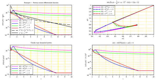
Figure 1. Convergence rates of values, trajectories and gradients.

4. Example for comparison of the convergence rate

Example 4.1.

Take $f:]-1,+\infty[^{2}\to{\mathbb{R}}$ which is defined by

$$f(x)=\frac{1}{2}(x_{1}+x_{2})^{2}-\ln(x_{1}+1)(x_{2}+1).$$

The function $f_{1}$ is strictly convex with gradient

$$\nabla f(x)=\begin{bmatrix}x_{1}+x_{2}-\frac{1}{x_{1}+1}\\ x_{1}+x_{2}-\frac{1}{x_{2}+1}\end{bmatrix}\text{ and Hessian }\nabla^{2}f(x)=\begin{bmatrix}1+\frac{1}{(x_{1}+1)^{2}}&1\\ 1&1+\frac{1}{(x_{2}+1)^{2}}\end{bmatrix}.$$

The unique minimizer of $f$ is $x^{*}=\left((\sqrt{3}-1)/2,(\sqrt{3}-1)/2\right)$. The corresponding trajectories to the system (3) are depicted in Figure 1. We note that the convergence rates of the values in this numerical test are consistent with those predicted in Corollaries 3.1 and 3.2, while the convergence rates of the gradients are clearly stronger than those predicted theoretically. Let us consider the times-second-order systems, treated in the very recent papers:

(TRAL) $$\dot{x}(t)+2t^{2}\ln^{2}t\nabla f\left(x(t)\right)+5x(t)=0,$$

(TRAE) $$\dot{x}(t)+2t^{2}e^{2t^{9/10}}\nabla f\left(x(t)\right)+5x(t)=0,$$

(TRISAL) $$\ddot{x}(t)+5\dot{x}(t)+2t^{2}\ln^{2}t\nabla f\left(x(t)\right)+5x(t)=0,\text{ see \cite[cite]{[\@@bibref{}{BCR1}{}{}]}},$$

(TRISAE) $$\ddot{x}(t)+5\dot{x}(t)+2t^{2}e^{2t^{4/5}}\nabla f\left(x(t)\right)+5x(t)=0,\text{ see \cite[cite]{[\@@bibref{}{BCR1}{}{}]}},$$

(TRISG) $$\ddot{x}(t)+5t^{-4/5}\dot{x}(t)+\nabla f\left(x(t)\right)+t^{-8/5}x(t)=0,\text{ see \cite[cite]{[\@@bibref{}{ABCR-JDE}{}{}]}},$$

(TRISH) $$\ddot{x}(t)+5t^{-4/5}\dot{x}(t)+\nabla f\left(x(t)\right)+2\nabla^{2}f\left(x(t)\right)\dot{x}(t)+t^{-8/5}x(t)=0,\text{ see \cite[cite]{[\@@bibref{}{ABCR-JDE}{}{}]}}.$$

By comparing the two times-first-order systems, (3) where $\beta(t)$ is either equal to $2t^{2}\ln^{2}t$ or $2t^{2}e^{2t^{9/10}}$, with those of second order, we are surprised (see Figure 3) by the better rate of convergence brought by these two reduced and inexpensive systems.

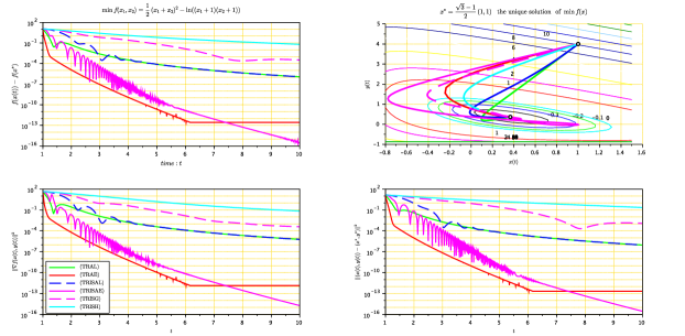
Figure 2. Convergence rates of values, trajectories and gradients.

5. Implicit discretization for nonsmooth convex functions

Here, we suppose $f:\,\mathcal{H}\rightarrow\mathbb{R}\cup\{+\infty\}$ to be a proper lower semicontinuous convex function. Let us recall that an implicit discretization of the dynamical system (3) with $\beta(k)=\dfrac{\beta_{k}}{d}>0$ and $d=1-c>0$ leads to the numerical scheme (5) that reads for every $k\geq k_{0}$

(31) $$x_{k+1}-x_{k}+\dfrac{\beta_{k}}{d}\partial\varphi_{k}(x_{k+1})=\frac{1}{d}\left(x_{k+1}+\beta_{k}\partial f(x_{k+1})-dx_{k}\right)\ni 0$$

$$\iff\;x_{k+1}=\text{prox}_{\frac{\beta_{k}}{d}\varphi_{k}}(x_{k})=\text{prox}_{\beta_{k}f}(dx_{k}),$$

where $\varphi_{k}:=f+\frac{1-d}{2\beta_{k}}\left\lVert\cdot\right\rVert^{2}$. We suppose the following condition:

$$(\mathbf{H}_{\beta_{k}}) (\beta_{k})\textit{ is a nondecreasing and satisfies }\,\underset{k\rightarrow+\infty}{\lim}\,\beta_{k}=+\infty.$$

For each $k\geq k_{0}$, we denote by $y_{k}$ the unique minimizer of the strongly convex function $\varphi_{k}$, which means by the first order convex optimality condition

(32) $$\partial f(y_{k})+\dfrac{1-d}{\beta_{k}}y_{k}\ni 0\;\iff\;y_{k}=\text{prox}_{\frac{1-d}{\beta_{k}}f}(0).$$

Let us recall (see [16, Prop 2.6] for general maximal monotone operators) that the Tikhonov approximation curve $k\mapsto y_{k}$ satisfies

(33) $$\forall k\geq k_{0},\;\;\left\lVert y_{k}\right\rVert\leq\left\lVert x^{*}\right\rVert\hbox{ and }\underset{k\rightarrow+\infty}{\lim}\left\lVert y_{k}-x^{*}\right\rVert=0.$$

Now, for $\lambda$ a positive constant, we introduce the following discrete energy function

(34) $$E_{k}=\beta_{k}\left(\varphi_{k}(x_{k})-\varphi_{k}(y_{k})\right)+\frac{\lambda}{2}\left\lVert x_{k}-y_{k-1}\right\rVert^{2},\;\;\text{for all }\,k\geq k_{0}.$$

Before giving this section’s principal theorem, we need two very important lemmas. The first lemma relates the asymptotic behavior of the sequence $E_{k}$ to the convergence rate of values and iterations, the second lemma provides a few properties of the viscosity curve $(y_{k})_{k}.$

Lemma 5.1.

Let $(x_{k})$ be the sequence generated by the algorithm (5). Then for any $k\geq k_{0}$ we have:

(35) $$f(x_{k})-\underset{\mathcal{H}}{\min}\,f\leq\dfrac{E_{k}}{\beta_{k}}+\dfrac{1-d}{2\beta_{k}}\left\lVert x^{*}\right\rVert^{2}$$

and

(36) $$\left\lVert x_{k}-y_{k}\right\rVert^{2}\leq\dfrac{2E_{k}}{1-d}.$$

Therefore, $x_{k}$ converges strongly to $x^{*}$ as soon as $\underset{k\rightarrow+\infty}{\lim}E_{k}=0$.

Proof.

Observing the definition of $\varphi_{k}$, one has

(37) $$f(x_{k})-\underset{\mathcal{H}}{\min}\,f = \varphi_{k}(x_{k})-\dfrac{1-d}{2\beta_{k}}\left\lVert x_{k}\right\rVert^{2}-\varphi_{k}(x^{*})+\dfrac{1-d}{2\beta_{k}}\left\lVert x^{*}\right\rVert^{2}$$

$$= \left[\varphi_{k}(x_{k})-\varphi_{k}(x_{\beta_{k}})\right]+\left[\underbrace{\varphi_{k}(y_{k})-\varphi_{k}(x^{*})}_{\leq 0}\right]$$

$$+\dfrac{1-d}{2\beta_{k}}\left\lVert x^{*}\right\rVert^{2}\underbrace{-\dfrac{1-d}{2\beta_{k}}\left\lVert x_{k}\right\rVert^{2}}_{\leq 0}$$

$$\leq \varphi_{k}(x_{k})-\varphi_{k}(y_{k})+\dfrac{1-d}{2\beta_{k}}\left\lVert x^{*}\right\rVert^{2}.$$

From definition of $E_{k}$, we obtain

(38) $$\varphi_{k}(x_{k})-\varphi_{k}(y_{k})\leq\dfrac{E_{k}}{\beta_{k}},$$

which, combined with (37), gives (35).
Using the strong convexity of $\varphi_{k}$, and $y_{k}:=\underset{\mathcal{H}}{{\rm argmin}\kern 1.19995pt}\,\varphi_{k}$, we obtain

$$\varphi_{k}(x_{k})-\varphi_{k}(y_{k})\geq\dfrac{1-d}{2\beta_{k}}\left\lVert x_{k}-y_{k}\right\rVert^{2}.$$

By combining the last inequality with (38), we get

$$\dfrac{E_{k}}{\beta_{k}}\geq\dfrac{1-d}{2\beta_{k}}\left\lVert x_{k}-y_{k}\right\rVert^{2},$$

which implies the inequality (36). Recall that $\underset{k\rightarrow+\infty}{\lim}\left\lVert y_{k}-x^{*}\right\rVert=0$, so according to $\underset{k\rightarrow+\infty}{\lim}E_{k}=0$, we deduce that the sequence $(x_{k})$ converges strongly to $x^{*}$. ∎

Lemma 5.2.

For every $k\geq k_{0}$, the following properties are satisfied:

• $\varphi_{k}(y_{k})-\varphi_{k+1}(y_{k+1})\leq\dfrac{(1-d)}{2}\left(\dfrac{1}{\beta_{k}}-\dfrac{1}{\beta_{k+1}}\right)\left\lVert y_{k+1}\right\rVert^{2},$

• $\left\lVert y_{k+1}-y_{k}\right\rVert^{2}\leq\dfrac{\beta_{k+1}-\beta_{k}}{\beta_{k+1}}\langle y_{k+1},y_{k+1}-y_{k}\rangle$, and

• $\left\lVert y_{k+1}-y_{k}\right\rVert\leq\dfrac{\beta_{k+1}-\beta_{k}}{\beta_{k+1}}\left\lVert y_{k+1}\right\rVert.$

Proof.

i) Recall that $y_{k}$ is the unique minimizer of the function $\varphi_{k}=f+\frac{1-d}{2\beta_{k}}\left\lVert\cdot\right\rVert^{2}$, then

$$\varphi_{k}(y_{k})\leq\varphi_{k}(y_{k+1})=f(y_{k+1})+\frac{1-d}{2\beta_{k}}\left\lVert y_{k+1}\right\rVert^{2},$$

and also

$$-\varphi_{k+1}(y_{k+1})=-f(y_{k+1})-\frac{1-d}{2\beta_{k+1}}\left\lVert y_{k+1}\right\rVert^{2}.$$

Summing these two inequalities, we get the first statement of this lemma.

ii) By (32), we have

$$\frac{d-1}{\beta_{k}}y_{k}\in\partial f(y_{k})\;\;\;\;\text{and}\;\;\;\;\frac{d-1}{\beta_{k+1}}y_{k+1}\in\partial f(y_{k+1}).$$

The monotonicity of $\partial f$ gives

$$\left\langle\frac{1-d}{\beta_{k}}y_{k}-\frac{1-d}{\beta_{k+1}}y_{k+1},y_{k+1}-y_{k}\right\rangle\geq 0,$$

it follows that

$$\frac{1-d}{\beta_{k}}\left\lVert y_{k+1}-y_{k}\right\rVert^{2}\leq\left(\dfrac{1-d}{\beta_{k}}-\dfrac{1-d}{\beta_{k+1}}\right)\langle y_{k+1},y_{k+1}-y_{k}\rangle,$$

which gives the second statement of this lemma. The last statement follows from Cauchy-Schwarz inequality. ∎

By adding the following hypothesis on $(\beta_{k})$:

$$(\mathbf{H}_{\beta_{k}}) \left\{\begin{array}[]{ll}(i)&\dot{\beta}_{k}:=\beta_{k+1}-\beta_{k}\neq 0,\text{ for }k\text{ large enough};\\ (ii)&\underset{k\rightarrow+\infty}{\lim}\,\dfrac{\dot{\beta}_{k+1}}{\dot{\beta}_{k}}=\underset{k\rightarrow+\infty}{\lim}\,\dfrac{\beta_{k+1}}{\beta_{k}}=\ell>0;\end{array}\right.$$

let us show the main result of this section.

Theorem 5.3.

Let $f:\mathcal{H}\rightarrow\mathbb{R}\cup\{+\infty\}$ be a proper lower semicontinuous convex function, with $\text{argmin}_{\mathcal{H}}f\neq\emptyset$, and $(x_{k})$ be a sequence generated by the algorithm (5). Let $\rho\in]0,1-d[$ and suppose the condition $(\mathbf{H}_{\beta_{k}})$. Then, we have

• for $k$ large enough

  $$f(x_{k})-\underset{\mathcal{H}}{\min}f=\mathcal{O}\left(\dfrac{1}{\beta_{k}}\right),\;\left\lVert\dot{x}_{k}\right\rVert^{2}=\mathcal{O}\left(\dfrac{\dot{\beta}_{k}}{\beta_{k}}+e^{-\rho k}\right)$$

  $$\text{ and }\left\lVert x_{k}-y_{k}\right\rVert^{2}=\mathcal{O}\left(\dfrac{\dot{\beta}_{k}}{\beta_{k}}+e^{-\rho k}\right);$$

• if $\ell=1$ in $(\mathbf{H}_{\beta_{k}})$, the sequence $(x_{k})$ generated by the algorithm (5) converges strongly to $x^{*}$ the element of minimum norm of $\text{argmin}_{\mathcal{H}}f$;

• for $k$ large enough

  $$d(0,\partial f(x_{k+1}))=\mathcal{O}\left(\dfrac{1}{\beta_{k}}\right),$$

  and then if $f$ is differentiable on $\mathcal{H}$, we have strong convergence of the gradients to zero with the rate

  (39) $$\left\lVert\nabla f(x_{k})\right\rVert=\mathcal{O}\left(\dfrac{1}{\beta_{k}}\right).$$

Proof.

To simplify the writing of the proof, we use the following notations: $v_{k}:=x_{k}-y_{k-1}$ and for any sequence $(u_{k})$ in $\mathcal{H}$, we write $\dot{u}_{k}:=u_{k+1}-u_{k}.$
From (34), we have

$$\begin{array}[]{lll}\dot{E}_{k}&\leq&\beta_{k+1}\left(\varphi_{k+1}(x_{k+1})-\varphi_{k+1}(y_{k+1})\right)-\beta_{k}\left(\varphi_{k}(x_{k})-\varphi_{k}(y_{k})\right)\\ \\ &&+\frac{\lambda}{2}\left(\left\lVert v_{k+1}\right\rVert^{2}-\left\lVert v_{k}\right\rVert^{2}\right)\\ \\ &=&\beta_{k}\left[\varphi_{k}(x_{k+1})-\varphi_{k}(x_{k})\right]+\dot{\beta}_{k}\left[\varphi_{k}(x_{k+1})-\varphi_{k}(y_{k})\right]\\ \\ &&+\beta_{k+1}\left[\varphi_{k+1}(x_{k+1})-\varphi_{k}(x_{k+1})+\varphi_{k}(y_{k})-\varphi_{k+1}(y_{k+1})\right]\\ \\ &&+\frac{\lambda}{2}\left(\left\lVert v_{k+1}\right\rVert^{2}-\left\lVert v_{k}\right\rVert^{2}\right).\end{array}$$

Using the definition of $\varphi_{k}$ and that $(\beta_{k})$ is nondecreasing, we deduce that

(40) $$\varphi_{k+1}(x_{k+1})-\varphi_{k}(x_{k+1})=\dfrac{1-d}{2}\left(\dfrac{1}{\beta_{k+1}}-\dfrac{1}{\beta_{k}}\right)\left\lVert x_{k+1}\right\rVert^{2}\leq 0;$$

so, according to Lemma 5.2 $i)$, we obtain

$$\begin{array}[]{lll}\dot{E}_{k}&\leq&\beta_{k}\left[\varphi_{k}(x_{k+1})-\varphi_{k}(x_{k})\right]+\dot{\beta}_{k}\left[\varphi_{k}(x_{k+1})-\varphi_{k}(y_{k})\right]\\ \\ &&+\dfrac{(1-d)}{2}\dfrac{\dot{\beta}_{k}}{\beta_{k}}\left\lVert y_{k+1}\right\rVert^{2}+\dfrac{\lambda}{2}\left(\left\lVert v_{k+1}\right\rVert^{2}-\left\lVert v_{k}\right\rVert^{2}\right).\end{array}$$

Noting that $\frac{\lambda}{2}\left(\left\lVert v_{k+1}\right\rVert^{2}-\left\lVert v_{k}\right\rVert^{2}\right)\leq\lambda\langle\dot{v}_{k},v_{k+1}\rangle$ then

(41) $$\begin{array}[]{lll}\dot{E}_{k}&\leq&\beta_{k}\left[\varphi_{k}(x_{k+1})-\varphi_{k}(x_{k})\right]+\dot{\beta}_{k}\left[\varphi_{k}(x_{k+1})-\varphi_{k}(y_{k})\right]\\ \\ &&+\dfrac{(1-d)\dot{\beta}_{k}}{2\beta_{k}}\left\lVert y_{k+1}\right\rVert^{2}+\lambda\langle\dot{v}_{k},v_{k+1}\rangle.\end{array}$$

Returning to form (4) of algorithm (5), we obtain

$$\begin{array}[]{lll}\dot{v}_{k}&=&v_{k+1}-v_{k}=x_{k+1}-y_{k}-x_{k}+y_{k-1}=\dot{x}_{k}-\dot{y}_{k-1}.\end{array}$$

Thus

(42) $$\lambda\langle\dot{v}_{k},v_{k+1}\rangle=\lambda\langle\dot{x}_{k},x_{k+1}-y_{k}\rangle-\lambda\langle\dot{y}_{k-1},x_{k+1}-y_{k}\rangle.$$

By strong convexity of $\varphi_{k}$ and $-\frac{d}{\beta_{k}}\dot{x}_{k}\in\partial\varphi_{k}(x_{k+1})$, we have

(43) $$\left\langle\frac{d}{\beta_{k}}\dot{x}_{k},x_{k+1}-y_{k}\right\rangle\leq-\left(\varphi_{k}(x_{k+1})-\varphi_{k}(y_{k})\right)-\frac{1-d}{2\beta_{k}}\left\lVert x_{k+1}-y_{k}\right\rVert^{2}.$$

Also, using Lemma 5.2 $ii)$ and inequality in (33), we have for any $b>0$

(44) $$\begin{array}[]{lll}-\lambda\langle\dot{y}_{k-1},x_{k+1}-y_{k}\rangle&\leq&\dfrac{\lambda b}{2}\left\lVert\dot{y}_{k-1}\right\rVert^{2}+\dfrac{\lambda}{2b}\left\lVert x_{k+1}-y_{k}\right\rVert^{2}\\ \\ &\leq&\dfrac{\lambda b}{2}\dfrac{\dot{\beta}^{2}_{k-1}}{\beta^{2}_{k}}\left\lVert x^{*}\right\rVert^{2}+\dfrac{\lambda}{2b}\left\lVert x_{k+1}-y_{k}\right\rVert^{2}.\end{array}$$

Combining (42), (43) and (44), we deduce

(45) $$\begin{array}[]{lll}\lambda\langle\dot{v}_{k},v_{k+1}\rangle&\leq&\dfrac{-\lambda\beta_{k}}{d}\left(\varphi_{k}(x_{k+1})-\varphi_{k}(y_{k})\right)+\dfrac{\lambda b}{2}\dfrac{\dot{\beta}^{2}_{k-1}}{\beta^{2}_{k}}\left\lVert x^{*}\right\rVert^{2}\\ \\ &&+\dfrac{\lambda}{2}\left(\dfrac{1}{b}-\dfrac{1-d}{d}\right)\left\lVert x_{k+1}-y_{k}\right\rVert^{2}.\end{array}$$

Using again the strong convexity of $\varphi_{k}$, we have

$$\varphi_{k}(x_{k})-\varphi_{k}(x_{k+1})\geq\left\langle\frac{d}{\beta_{k}}\dot{x}_{k},x_{k+1}-x_{k}\right\rangle+\dfrac{1-d}{2\beta_{k}}\left\lVert x_{k+1}-x_{k}\right\rVert^{2}=\dfrac{1+d}{2\beta_{k}}\left\lVert\dot{x}_{k}\right\rVert^{2},$$

which implies

(46) $$\begin{array}[]{lll}\beta_{k}\left(\varphi_{k}(x_{k+1})-\varphi_{k}(x_{k})\right)&\leq&-\dfrac{1+d}{2}\left\lVert\dot{x}_{k}\right\rVert^{2}\leq 0.\end{array}$$

Returning to (41),(45),(46) and using $\left\lVert y_{k+1}\right\rVert\leq\left\lVert x^{*}\right\rVert$, we obtain

(47) $$\begin{array}[]{lll}\dot{E}_{k}&\leq&\frac{\lambda}{2}\left(\frac{1}{b}-\frac{1-d}{d}\right)\left\lVert x_{k+1}-y_{k}\right\rVert^{2}+\frac{1}{2}\left(\lambda b\frac{\dot{\beta}^{2}_{k-1}}{\beta^{2}_{k}}+(1-d)\frac{\dot{\beta}_{k}}{\beta_{k}}\right)\left\lVert x^{*}\right\rVert^{2}\\ \\ &&+\left(\beta_{k+1}-(1+\frac{\lambda}{d})\beta_{k}\right)\left[\varphi_{k}(x_{k+1})-\varphi_{k}(y_{k})\right].\end{array}$$

Set $\mu:=\frac{\rho}{1-\rho}$, then $\mu\in\left]0,\frac{1-d}{d}\right[$, and according to the definition of $E_{k}$, we get

$$\begin{array}[]{lll}\mu E_{k+1}&=&\mu\beta_{k+1}\left(\varphi_{k+1}(x_{k+1})-\varphi_{k+1}(y_{k+1})\right)+\dfrac{\mu\lambda}{2}\left\lVert x_{k+1}-y_{k}\right\rVert^{2}\\ \\ &=&\mu\beta_{k+1}\left(\varphi_{k}(x_{k+1})-\varphi_{k}(y_{k})\right)+\dfrac{\mu\lambda}{2}\left\lVert x_{k+1}-y_{k}\right\rVert^{2}\\ \\ &&+\mu\beta_{k+1}\left(\varphi_{k+1}(x_{k+1})-\varphi_{k}(x_{k+1})+\varphi_{k}(y_{k})-\varphi_{k+1}(y_{k+1})\right)\end{array}$$

Using (40) and Lemma 5.2 $i)$, we obtain

(48) $$\begin{array}[]{lll}\mu E_{k+1}&\leq&\mu\beta_{k+1}\left(\varphi_{k}(x_{k+1})-\varphi_{k}(y_{k})\right)+\dfrac{\mu(1-d)\dot{\beta}_{k}}{2\beta_{k}}\left\lVert x^{*}\right\rVert^{2}\\ \\ &&+\dfrac{\mu\lambda}{2}\left\lVert x_{k+1}-y_{k}\right\rVert^{2}.\end{array}$$

Adding (47) and (48), we conclude

(49) $$\dot{E}_{k}+\mu E_{k+1} \leq \dfrac{\lambda}{2}\left(\underbrace{\dfrac{1}{b}-\dfrac{1-d}{d}+\mu}_{A}\right)\left\lVert x_{k+1}-y_{k}\right\rVert^{2}$$

$$+\dfrac{1}{2}\left(\lambda b\dfrac{\dot{\beta}^{2}_{k-1}}{\beta^{2}_{k}}+(1-d)(1+\mu)\dfrac{\dot{\beta}_{k}}{\beta_{k}}\right)\left\lVert x^{*}\right\rVert^{2}$$

$$+\left(\underbrace{(1+\mu)\beta_{k+1}-\left(1+\frac{\lambda}{d}\right)\beta_{k}}_{B}\right)\left(\varphi_{k}(x_{k+1})-\varphi_{k}(y_{k})\right).$$

Choosing $\lambda$ such that for all $k$: ${\lambda>d\left((1+\mu)\dfrac{\beta_{k+1}}{\beta_{k}}-1\right)}$, which is valid since $\left(\frac{\beta_{k+1}}{\beta_{k}}\right)$ is bounded, we get

$$B=\dfrac{\beta_{k}}{d}\left(d\left((1+\mu)\dfrac{\beta_{k+1}}{\beta_{k}}-1\right)-\lambda\right)\leq 0.$$

Choosing also $b=\dfrac{d}{1-(1+\mu)d}$, which is positive since $\mu<\frac{1-d}{d}$, we cancel the term $A$ in inequality (49). Consequently, for all $k\geq k_{0}$

(50) $$\dot{E}_{k}+\mu E_{k+1}\leq\gamma_{k}\left\lVert x^{*}\right\rVert^{2}$$

with

$$\gamma_{k}:=\dfrac{1}{2}\left(\dfrac{\lambda d}{1-(1+\mu)d}\dfrac{\dot{\beta}^{2}_{k-1}}{\beta^{2}_{k}}+(1-d)(1+\mu)\dfrac{\dot{\beta}_{k}}{\beta_{k}}\right).$$

Inequality (50) is equivalent to

$$E_{k+1}+\left(\dfrac{\mu}{1+\mu}-1\right)E_{k}\leq\left(1-\dfrac{\mu}{1+\mu}\right)\gamma_{k}\left\lVert x^{*}\right\rVert^{2}.$$

Multiplying the last inequality by $e^{\rho(k+1)}$ and using $\rho=\dfrac{\mu}{1+\mu}$, we obtain

$$e^{\rho(k+1)}E_{k+1}+(\rho-1)e^{\rho(k+1)}E_{k}\leq(1-\rho)e^{\rho(k+1)}\gamma_{k}\left\lVert x^{*}\right\rVert^{2}.$$

Hence, for all $k\geq k_{0}$

$$e^{\rho(k+1)}E_{k+1}-e^{\rho k}E_{k}+(e^{-\rho}+\rho-1)e^{\rho(k+1)}E_{k}\leq(1-\rho)e^{\rho(k+1)}\gamma_{k}\left\lVert x^{*}\right\rVert^{2}.$$

Remarking the function $y\mapsto e^{-y}+y-1$ is nonnegative on ${\mathbb{R}}_{+}$, we conclude that, for all $k\geq k_{0}$,

(51) $$e^{\rho(k+1)}E_{k+1}-e^{\rho k}E_{k}\leq me^{\rho(k+1)}\dfrac{\dot{\beta}_{k}}{\beta_{k}}\left(r\left(\dfrac{\dot{\beta}_{k-1}}{\dot{\beta}_{k}}\right)^{2}\dfrac{\dot{\beta}_{k}}{\beta_{k}}+1\right),$$

with $r:=\dfrac{\lambda d}{(1-\rho-d)(1-d)}$ and $m:=\frac{1}{2}(1-\rho)(1-d)(1+\mu)\left\lVert x^{*}\right\rVert^{2}$.
Using the assumption $(\mathbf{H}_{\beta_{k}})$, we justify

$$\underset{k\to+\infty}{\lim}\frac{\dot{\beta}_{k}}{\beta_{k}}=\underset{k\to+\infty}{\lim}\left(\frac{\beta_{k+1}}{\beta_{k}}-1\right)=\ell-1\hbox{ and }\underset{k\to+\infty}{\lim}\frac{\dot{\beta}_{k}}{\dot{\beta}_{k+1}}\frac{\beta_{k+1}}{\beta_{k}}=1.$$

Thus, we have

$$\underset{k\to+\infty}{\lim}\dfrac{e^{\rho(k+1)}\dfrac{\dot{\beta}_{k}}{\beta_{k}}\left(r\left(\dfrac{\dot{\beta}_{k-1}}{\dot{\beta}_{k}}\right)^{2}\dfrac{\dot{\beta}_{k}}{\beta_{k}}+1\right)}{\dfrac{\dot{\beta}_{k+1}}{\beta_{k+1}}e^{\rho(k+2)}-\dfrac{\dot{\beta}_{k}}{\beta_{k}}e^{\rho(k+1)}} = \underset{k\to+\infty}{\lim}\dfrac{r\left(\dfrac{\dot{\beta}_{k-1}}{\dot{\beta}_{k}}\right)^{2}\dfrac{\dot{\beta}_{k}}{\beta_{k}}+1}{\dfrac{\beta_{k}}{\beta_{k+1}}\dfrac{\dot{\beta}_{k}}{\dot{\beta}_{k+1}}e^{\rho}-1}$$

$$= \dfrac{\dfrac{r(\ell-1)}{\ell^{2}}+1}{e^{\rho}-1}<+\infty.$$

Therefore, there exist $M>0$ and $k_{1}\geq k_{0}$ such that for $k\geq k_{1}$

(52) $$me^{\rho(k+1)}\dfrac{\dot{\beta}_{k}}{\beta_{k}}\left(r\left(\frac{\dot{\beta}_{k-1}}{\dot{\beta}_{k}}\right)^{2}\dfrac{\dot{\beta}_{k}}{\beta_{k}}+1\right)\leq M\left(\dfrac{\dot{\beta}_{k+1}}{\beta_{k+1}}e^{\rho(k+2)}-\dfrac{\dot{\beta}_{k}}{\beta_{k}}e^{\rho(k+1)}\right).$$

We conclude, for all $k\geq k_{1}$,

(53) $$e^{\rho(k+1)}E_{k+1}-e^{\rho k}E_{k}\leq M\left(\dfrac{\dot{\beta}_{k+1}}{\beta_{k+1}}e^{\rho(k+2)}-\dfrac{\dot{\beta}_{k}}{\beta_{k}}e^{\rho(k+1)}\right).$$

After summing the inequalities (53) between $k_{1}$ and $k>k_{1}$, and dividing by $e^{\rho(k+1)}$ we get

$$\begin{array}[]{lll}E_{k+1}&\leq&\dfrac{e^{\rho k_{1}}E_{k_{1}}}{e^{\rho(k+1)}}+\dfrac{M}{e^{\rho(k+1)}}\sum\limits_{j=k_{1}}^{k}\left(\dfrac{\dot{\beta}_{j+1}}{\beta_{j+1}}e^{\rho(j+2)}-\dfrac{\dot{\beta}_{j}}{\beta_{j}}e^{\rho(j+1)}\right)\\ &=&\dfrac{e^{\rho k_{1}}E_{k_{1}}}{e^{\rho(k+1)}}+\dfrac{M}{e^{\rho(k+1)}}\left(\dfrac{\dot{\beta}_{k+1}}{\beta_{k+1}}e^{\rho(k+2)}-\dfrac{\dot{\beta}_{k_{1}}}{\beta_{k_{1}}}e^{\rho(k_{1}+1)}\right)\\ &\leq&\dfrac{e^{\rho k_{1}}E_{k_{1}}}{e^{\rho(k+1)}}+Me^{\rho}\dfrac{\dot{\beta}_{k+1}}{\beta_{k+1}}.\end{array}$$

Consequently, for $k$ large enough

(54) $$E_{k}=\mathcal{O}\left(\dfrac{\dot{\beta}_{k}}{\beta_{k}}+e^{-\rho k}\right).$$

i) Return to (35) and using boundedness of the sequence $\left(\frac{\dot{\beta}_{k}}{\beta_{k}}\right)_{k}$ we have $(E_{k})$ is bounded, and thus

$$f(x_{k})-\underset{\mathcal{H}}{\min}\,f=\mathcal{O}\left(\dfrac{1}{\beta_{k}}\right).$$

Combining (36) and (46) with (54) we get for $k$ large enough

(55) $$\left\lVert\dot{x}_{k}\right\rVert^{2}=\mathcal{O}\left(\dfrac{\dot{\beta}_{k}}{\beta_{k}}+e^{-\rho k}\right)\text{ and }\left\lVert x_{k}-y_{k}\right\rVert^{2}=\mathcal{O}\left(\dfrac{\dot{\beta}_{k}}{\beta_{k}}+e^{-\rho k}\right).$$

ii) We have

$$\lim_{k\rightarrow+\infty}\dfrac{\dot{\beta}_{k}}{\beta_{k}}=\lim_{k\rightarrow+\infty}\dfrac{{\beta}_{k+1}}{\beta_{k}}-1=\ell-1=0,$$

then $x_{k}-y_{k}$ strongly converges to the origine of $\mathcal{H}$. Return to (33), we conclude that $x_{k}$ strongly converges to $x^{*}$.

iii) According to (4), let $z_{k}\in\partial f(x_{k+1})$ satisfying $x_{k+1}+\beta_{k}z_{k}-dx_{k}=0$. Then

$$d(0,\partial f(x_{k+1}))^{2} \leq \|z_{k}\|^{2}=\left\lVert\frac{d}{\beta_{k}}\dot{x}_{k}+\frac{1-d}{\beta_{k}}x_{k+1}\right\rVert^{2}$$

$$\leq \frac{2d^{2}}{\beta_{k}^{2}}\left\lVert\dot{x}_{k}\right\rVert^{2}+\frac{2(1-d)^{2}}{\beta_{k}^{2}}\left\lVert x_{k+1}\right\rVert^{2}.$$

Hence, (55) and boundedness of $(x_{k})$ lead to

$$d(0,\partial f(x_{k+1}))=\mathcal{O}\left(\dfrac{1}{\beta_{k}}\right),\text{ for $k$ large enough}.$$

If in addition $f$ is differentiable, we obtain the large convergence rate (39). ∎

6. Application to special cases

In this section we review two special cases for the sequence $(\beta_{k})$.

6.1. Case $\beta_{k}=k^{m}\ln^{q}(k)$:

To investigate the fulfillment of the condition $(\mathbf{H}_{\beta_{k}})$, let us first note that for $a>0$ and for $k$ large enough we have

$$\;\left(1+\frac{a}{k}\right)^{m}=1+\frac{am}{k}+o\left(\frac{1}{k}\right)\;\;\text{ and }\;\;\ln\left(1+\frac{a}{k}\right)=\frac{a}{k}+o\left(\frac{1}{k}\right).$$

Then

$$\left(1+\frac{a}{k}\right)^{m}\left(1+\frac{\ln(1+\frac{a}{k})}{\ln(k)}\right)^{q} = \left(1+\frac{am}{k}+o\left(\frac{1}{k}\right)\right)\left(1+\frac{a}{k\ln(k)}+o\left(\frac{1}{k\ln(k)}\right)\right)^{q}$$

$$= \left(1+\frac{am}{k}+o\left(\frac{1}{k}\right)\right)\left(1+\frac{aq}{k\ln(k)}+o\left(\frac{1}{k\ln(k)}\right)\right);$$

which gives

(56) $$\left(1+\frac{a}{k}\right)^{m}\left(1+\frac{\ln(1+\frac{a}{k})}{\ln(k)}\right)^{q}=1+\frac{am}{k}+\frac{aq}{k\ln(k)}+o\left(\frac{1}{k\ln(k)}\right).$$

• For $(\mathbf{H}_{\beta_{k}})$(i), we have $\dot{\beta}_{k}\neq 0\textit{ for }k>1$, which is trivial.
  

• For $(\mathbf{H}_{\beta_{k}})$(ii), we come back to (56) to deduce that when $k$ is large enough

  $$\dfrac{\beta_{k+1}}{\beta_{k}} = \dfrac{(k+1)^{m}\ln^{q}(k+1)}{k^{m}\ln^{q}(k)}$$

  $$= \left(1+\dfrac{1}{k}\right)^{m}\left(1+\dfrac{\ln(1+\frac{1}{k})}{\ln(k)}\right)^{q}$$

  $$= 1+\frac{m}{k}+\frac{q}{k\ln(k)}+o\left(\frac{1}{k\ln(k)}\right).$$

  Thus $\lim_{k\rightarrow+\infty}\dfrac{\beta_{k+1}}{\beta_{k}}=1>0$.
  We also remark that

  $$\begin{array}[]{lll}\dfrac{\dot{\beta}_{k+1}}{\dot{\beta}_{k}}&=&\dfrac{(k+2)^{m}\ln^{q}(k+2)-(k+1)^{m}\ln^{q}(k+1)}{(k+1)^{m}\ln^{q}(k+1)-k^{m}\ln^{q}(k)}\\ \\ &=&\dfrac{\left(1+\frac{2}{k}\right)^{m}\left(1+\frac{\ln(1+\frac{2}{k})}{\ln(k)}\right)^{q}-\left(1+\frac{1}{k}\right)^{m}\left(1+\frac{\ln(1+\frac{1}{k})}{\ln(k)}\right)^{q}}{\left(1+\frac{1}{k}\right)^{m}\left(1+\frac{\ln(1+\frac{1}{k})}{\ln(k)}\right)^{q}-1}.\end{array}$$

  Then, using (56), we get for $k$ large enough

  $$\begin{array}[]{lll}\dfrac{\dot{\beta}_{k+1}}{\dot{\beta}_{k}}&=&\dfrac{\!\left(\!1+\frac{2m}{k}+\frac{2q}{k\ln(k)}+o\left(\!\frac{1}{k\ln(k)}\!\right)\right)-\left(\!1+\frac{m}{k}+\frac{q}{k\ln(k)}+o\left(\frac{1}{k\ln(k)}\!\right)\!\right)}{\left(\!1+\frac{m}{k}+\frac{q}{k\ln(k)}+o\!\left(\!\frac{1}{k\ln(k)}\!\right)\!\right)-1}\\ &=&\dfrac{m\ln(k)+q+o(1)}{m\ln(k)+q+o(1)}.\end{array}$$

  Thus, for $(m,q)\in(\mathbb{R}^{+})^{2}\setminus\{(0,0)\}$, we deduce $\underset{k\to+\infty}{\lim}\dfrac{\dot{\beta}_{k+1}}{\dot{\beta}_{k}}=1.$

Consequently all conditions of $(\mathbf{H}_{\beta_{k}})$ are satisfied. So, based on Theorem 5.3, the following result can be proved easily.

Proposition 6.1.

Let $f$ and $(x_{k})$ be as in Theorem 5.3, and $\beta_{k}=k^{m}\ln^{q}(k)$ where $(m,q)\in(\mathbb{R}^{+})^{2}\setminus\{(0,0)\}$. Then $(x_{k})$ converges strongly to $x^{*}$ the element of minimum norm of $\text{argmin}_{\mathcal{H}}f$ and

$$f(x_{k})-\underset{\mathcal{H}}{\min}f=\mathcal{O}\left(\frac{1}{k^{m}\ln^{q}(k)}\right);\;\;\;\;\left\lVert\dot{x}_{k}\right\rVert^{2}=\left\{\begin{array}[]{lcl}\mathcal{O}\left(\frac{1}{k}\right)&\textit{ if }\;r\neq 0&\\ \mathcal{O}\left(\frac{1}{k\ln(k)}\right)&\textit{ if }\;r=0;&\\ \end{array}\right.$$

$$d(0,\partial f(x_{k}))=\mathcal{O}\left(\frac{1}{k^{m}\ln^{q}(k)}\right).$$

If moreover $f$ is differentiable, then

$$\;\left\lVert\nabla f(x_{k})\right\rVert=\mathcal{O}\left(\dfrac{1}{k^{m}\ln^{q}(k)}\right).$$

6.2. Case $\beta_{k}=k^{m}e^{\gamma k^{r}}$: 

Let us now treat the case $\beta_{k}=k^{m}e^{\gamma k^{r}}$ with $r\in]0,1],m\geq 0$ and $\gamma>0$. To fulfill the condition $(\mathbf{H}_{\beta_{k}})$, we first remark that for $0<r<1$ and $a>0$ we have for $k$ large enough

$$(k+a)^{r}-k^{r}=k^{r}\left[\left(1+\dfrac{a}{k}\right)^{r}-1\right]=ark^{r-1}+o(k^{r-1}).$$

Hence, for $k$ large enough

(58) $$e^{\gamma((k+a)^{r}-k^{r})}=e^{a\gamma rk^{r-1}+o(k^{r-1})}=1+a\gamma rk^{r-1}+o(k^{r-1}).$$

• Likewise $(\mathbf{H}_{\beta_{k}})$(i), $\dot{\beta}_{k}\neq 0\textit{ for }k>1$ is trivial.

• For $(\mathbf{H}_{\beta_{k}})$(ii), we distinguish two cases:

  $\star$ If $0<r<1$ then using (58) with $a=1$, we get for $k$ large enough

  $$\dfrac{\beta_{k+1}}{\beta_{k}}=\left(1+\frac{1}{k}\right)^{m}e^{\gamma\left((k+1)^{r}-k^{r}\right)}=1+\gamma rk^{r-1}+o(k^{r-1}),$$

  $$\begin{array}[]{lll}\dfrac{\dot{\beta}_{k+1}}{\dot{\beta}_{k}}&=&\dfrac{(k+2)^{m}e^{\gamma(k+2)^{r}}-(k+1)^{m}e^{\gamma(k+1)^{r}}}{(k+1)^{m}e^{\gamma(k+1)^{r}}-k^{m}e^{\gamma k^{r}}}\\ \\ &=&\dfrac{1+\frac{m}{\gamma rk^{r}}+o\left(\frac{m}{k^{-r}}\right)}{1+\frac{m}{\gamma rk^{r}}+o\left(\frac{m}{k^{-r}}\right)}.\end{array}$$

  Thus

  $$\underset{k\to+\infty}{\lim}\dfrac{{\beta}_{k+1}}{{\beta}_{k}}=\underset{k\to+\infty}{\lim}\dfrac{\dot{\beta}_{k+1}}{\dot{\beta}_{k}}=1>0.$$

  $\star$ If $r=1$, we have for $k$ large enough the termes $\dfrac{\beta_{k+1}}{\beta_{k}}$ and $\dfrac{\dot{\beta}_{k+1}}{\dot{\beta}_{k}}$ are equivalent to $e^{\gamma}\left(1+\frac{m}{k}+o\left(\frac{1}{k}\right)\right)$, so

  $$\underset{k\to+\infty}{\lim}\dfrac{{\beta}_{k+1}}{{\beta}_{k}}=\underset{k\to+\infty}{\lim}\dfrac{\dot{\beta}_{k+1}}{\dot{\beta}_{k}}=e^{\gamma}>0.$$

Applying again Theorem 5.3, we get the following Corollary.

Proposition 6.2.

Let $f$ and $(x_{k})$ be as in Theorem 5.3, where $\beta_{k}=k^{m}e^{\gamma k^{r}}.$ Then

$\star$ if $r=1$ and $m=0$, we have $(x_{k})$ is bounded and for $k$ large enough

$$f(x_{k})-\underset{\mathcal{H}}{\min}f=\mathcal{O}\left(e^{-\gamma k}\right);$$

$\star$ if either $0<r<1$ or $m>0$, $(x_{k})$ converges strongly to $x^{*}$ the element of minimum norm of $\text{argmin}_{\mathcal{H}}f$, and for $k$ large enough, we have

$$f(x_{k})-\underset{\mathcal{H}}{\min}f=\mathcal{O}\left(k^{-m}e^{-\gamma k^{r}}\right),\;\left\lVert\dot{x}_{k}\right\rVert^{2}=\mathcal{O}\left(\dfrac{1}{k^{1-r}}\right)\;$$

$$d(0,\partial f(x_{k}))=\mathcal{O}\left(k^{-m}e^{-\gamma k^{r}}\right).$$

If moreover $f$ is differentiable, then

$$\text{and }\;\left\lVert{\nabla}f(x_{k})\right\rVert=\mathcal{O}\left(k^{-m}e^{-\gamma k^{r}}\right).$$

7. Numerical example

In this section, we present a numerical example in the framework of nondifferentiable minimization problem to illustrate the performance of our iterative method (5). So, we consider the proper lower semicontinuous and convex function

$$f(x,y)=|x|+\iota_{[-a,a]}(x)+\frac{1}{2}(y-v_{0})^{2}$$

where $a>0,v_{0}\in\mathbb{R}$ and $\iota_{[-a,a]}$ is the indicator function having the value $0$ on $[-a,a]$ and $+\infty$ elsewhere. The well-known Fermat’s and subdifferential sum rules for convex functions ensure that $(\bar{x},\bar{y})\in\text{argmin}_{\mathbb{R}^{2}}f,$ iff

$$(0,0)\in\partial f(\bar{x},\bar{y})=\partial\left(|\cdot|+\delta_{[-a,a]}\right)(\bar{x})\times\partial\left(\frac{1}{2}(\cdot-v_{0})^{2}\right)(\bar{y})\iff(\bar{x},\bar{y})=(0,v_{0}).$$

Thus $\text{argmin}_{\mathbb{R}^{2}}f=\{0,v_{0})\}$. Using the rules for calculating proximal operators, see [14, Chap 6], we have for each $\lambda>0,(x,y)\in\mathbb{R}^{2}$,

$$\text{prox}_{\lambda f}(x,y) = \left(\text{prox}_{\lambda\left(|\cdot|+\delta_{[-a,a]}\right)}(x)\,,\,\text{prox}_{\lambda\left(\frac{1}{2}(\cdot-v_{0})^{2}\right)}(y)\right)$$

$$= \left(\min[\max(|x|-\lambda,0),a]\text{sign}(x)\;,\;-\frac{1}{\lambda+1}(y-\lambda v_{0})\right)$$

Below, we explain our algorithm (5) and the one proposed by László in the recent paper [23]:

(61) $$\left\{\begin{array}[]{rll}(x_{0},y_{0})&\in&\mathbb{R}^{2},\\ (x_{k+1},y_{k+1})&=&\text{prox}_{\beta_{k}f}(dx_{k},dy_{k})\end{array}\right.$$

(65) $$\left\{\begin{array}[]{rll}(x_{0},y_{0})&,&(x_{1},y_{1})\in\mathbb{R}^{2},\\ (u_{k},v_{k})&=&(x_{k},y_{k})+(1-\frac{\alpha}{k^{q}})(x_{k}-x_{k-1},y_{k}-y_{k-1}),\\ (x_{k+1},y_{k+1})&=&\text{prox}_{\lambda_{k}f}\left((u_{k},v_{k})-\frac{c}{k^{p}}(x_{k},y_{k})\right)\end{array}\right.$$

We note that (65) is an implicit discretization of the differentiable dynamical system studied in [22], that is $\ddot{x}(t)+\frac{\alpha}{t^{q}}\dot{x}(t)+\nabla f(x(t))+\frac{c}{t^{p}}x(t)=0$ where $\alpha,c,q,p>0$. In [23, Theorem 1.1], for $\lambda_{k}=\lambda k^{\delta}$, the conditions on the parameters $p,q,\alpha,\delta,\lambda$ and $c$ impose that $0<q<1,p\leq 2,\lambda>0,\delta\in\mathbb{R},c>0$ where the choice of $\delta,\lambda$ and $c$ depend on the positioning of $p$ with respect to $q+1$.

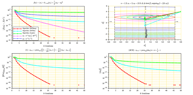
Figure 3. Comparison of convergence rates between the (61) algorithm and that of László.

The squared distance of $(x_{k},y_{k})$, generated by the above two iterations, to the solution $(x^{*},y^{*})$ and the decay of the objective function $f(x_{k},y_{k})-\min_{\mathbb{R}^{2}}f(x,y)$ along the iterations are shown in Figure 3 for the selected values $\beta_{k}$ equal respectively to $k^{3}\ln^{3}k$ and $k^{3}e^{2k^{4/5}}$ for the algorithm (61), and those equal to $p=2,q=\frac{4}{5},\alpha=2,\delta=2,\lambda=5$ for the algorithm (65). We note that the choice of $\beta_{k}=k^{3}e^{2k^{4/5}}$ justifies the originality of Theorem 5.3, since we end up with an exponential convergence rate for the values and the gradient. Also, the benefit of the inverse-relaxation $\beta_{k}=k^{3}e^{2k^{4/5}}$ (red curve in Figure 3), as allowed in Proposition 6.2, is clearly visible.

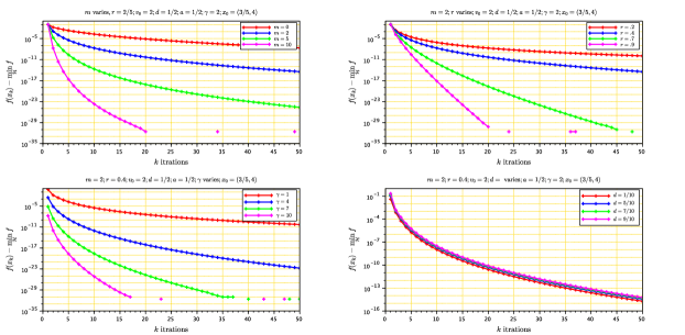
Figure 4. Convergence rates of values, trajectories and gradients.

Figure 4 explains the interest in the growth of the three parameters $m,r,\gamma$ in $\beta_{k}=k^{m}e^{\gamma k^{r}}$, while the parameter $d$ in Algorithm (5) does not act on the convergence rates.

8. Appendix

We rely on the basic properties of the Moreau envelope $f_{\gamma}:\mathcal{H}\longrightarrow\mathbb{R}\;\;(\gamma>0)$, which is defined by

(66) $$f_{\gamma}(x)={\min}_{y\in\mathcal{H}}\left(f(y)+\frac{1}{2\gamma}\left\lVert x-y\right\rVert^{2}\right)\;\;\text{for any }x\in\mathcal{H}.$$

Recall that, the functions $f$ and $f_{\lambda}$ share the same optimal objective value and the same set of minimizers

$${\min}_{y\in\mathcal{H}}\,f={\min}_{y\in\mathcal{H}}\,f_{\gamma}\;\;\;\;\;\;\text{and}\;\;\;\;\;\;{{\rm argmin}\kern 1.19995pt}_{\mathcal{H}}\,f={{\rm argmin}\kern 1.19995pt}_{\mathcal{H}}\,f_{\gamma}.$$

In addition, $f_{\lambda}$ is convex and continuously differentiable whose gradient is $\frac{1}{\gamma}$-Lipschitz continuous.

Lemma 8.1 ([2], [13, Section 12], [16]).

The unique point where the minimum value is achieved in (66) is denoted by ${\operatorname*{prox}}_{\gamma f}(x)$, and satisfies the following classical formulas: For each $\gamma>0$ and $x\in\mathcal{H}$,

• $f_{\gamma}(x)=f({\operatorname*{prox}}_{\gamma f}(x))+\frac{1}{2\gamma}\left\lVert x-{\operatorname*{prox}}_{\gamma f}(x)\right\rVert^{2}$;

• $\nabla f_{\gamma}(x)=\frac{1}{\gamma}(x-{\operatorname*{prox}}_{\gamma f}(x))$;

• ${\operatorname*{prox}}_{\theta f_{\gamma}}(x)=\frac{\gamma}{\gamma+\theta}x+\frac{\theta}{\gamma+\theta}{\operatorname*{prox}}_{(\gamma+\theta)f}(x),\;\text{ for all }\theta>0$;

• $\|{\operatorname*{prox}}_{\gamma f}(0)\|\leq\|x^{*}\|$, where $x^{*}=\mbox{\rm proj}_{{\rm argmin}\kern 0.83997ptf}0$;

• $\lim_{\gamma\rightarrow+\infty}\|{\operatorname*{prox}}_{\gamma f}(0)-x^{*}\|=0$.

The following Lemma provides an extended version of the classical gradient lemma which is valid for differentiable convex functions. The following version has been obtained in [5, Lemma 1], [6]. We reproduce its proof for the convenience of the reader.

Lemma 8.2.

Let $f:\mathcal{H}\to{\mathbb{R}}$ be a convex function whose gradient is $L$-Lipschitz continuous. Let $s\in]0,1/L]$. Then for all $(x,y)\in\mathcal{H}^{2}$, we have

(67) $$f(y-s\nabla f(y))\leq f(x)+\left\langle\nabla f(y),y-x\right\rangle-\frac{s}{2}\|\nabla f(y)\|^{2}-\frac{s}{2}\|\nabla f(x)-\nabla f(y)\|^{2}.$$

In particular, when ${\rm argmin}\kern 1.19995ptf\neq\emptyset$, we obtain that for any $x\in\mathcal{H}$

(68) $$f(x)\geq\min_{\mathcal{H}}f+\frac{1}{2L}\|\nabla f(x)\|^{2}.$$

Proof.

Denote $y^{+}=y-s\nabla f(y)$. By the standard descent lemma applied to $y^{+}$ and $y$, and since $sL\leq 1$ we have

(69) $$f(y^{+})\leq f(y)-\frac{s}{2}\left(2-Ls\right)\|\nabla f(y)\|^{2}\leq f(y)-\frac{s}{2}\|\nabla f(y)\|^{2}.$$

We now argue by duality between strong convexity and Lipschitz continuity of the gradient of a convex function. Indeed, using Fenchel identity, we have

$$f(y)=\langle\nabla f(y),\,y\rangle-f^{*}(\nabla f(y)).$$

$L$-Lipschitz continuity of the gradient of $f$ is equivalent to $1/L$-strong convexity of its conjugate $f^{*}$. This together with the fact that $(\nabla f)^{-1}=\partial f^{*}$ gives for all $(x,y)\in\mathcal{H}^{2}$,

$$f^{*}(\nabla f(y))\geq f^{*}(\nabla f(x))+\langle x,\,\nabla f(y)-\nabla f(x)\rangle+\frac{1}{2L}\left\lVert\nabla f(x)-\nabla f(y)\right\rVert^{2}.$$

Inserting this inequality into the Fenchel identity above yields

$$f(y) \leq-f^{*}(\nabla f(x))+\langle\nabla f(y),\,y\rangle-\langle x,\,\nabla f(y)-\nabla f(x)\rangle-\frac{1}{2L}\left\lVert\nabla f(x)-\nabla f(y)\right\rVert^{2}$$

$$=-f^{*}(\nabla f(x))+\langle x,\,\nabla f(x)\rangle+\langle\nabla f(y),\,y-x\rangle-\frac{1}{2L}\left\lVert\nabla f(x)-\nabla f(y)\right\rVert^{2}$$

$$=f(x)+\langle\nabla f(y),\,y-x\rangle-\frac{1}{2L}\left\lVert\nabla f(x)-\nabla f(y)\right\rVert^{2}$$

$$\leq f(x)+\langle\nabla f(y),\,y-x\rangle-\frac{s}{2}\left\lVert\nabla f(x)-\nabla f(y)\right\rVert^{2}.$$

Inserting the last bound into (69) completes the proof. ∎

References

[1] H. Attouch, Variational Convergence for Functions and Operators, Appl. Math. Ser., Pitman Advanced Publishing Program, Boston, 1984.
[2]H. Attouch, Viscosity solutions of minimization problems, SIAM J. Optim. 6 (3) (1996), 769–806.
[3]H. Attouch, A. Balhag, Z. Chbani and H. Riahi,
Damped inertial dynamics with vanishing Tikhonov regularization: Strong asymptotic convergence towards the minimum norm solution,
J. Differential Equations, 311 (2022), 29-58.
[4]H. Attouch, A. Balhag, Z. Chbani, H. Riahi, Fast convex optimization via inertial dynamics combining viscous and Hessian-driven damping with time rescaling, Evol.Equ. Control Theory 11 (2022), no. 2, 487-514.
[5]H. Attouch, Z. Chbani, J. Fadili, H. Riahi, First order optimization algorithms via inertial systems with Hessian driven damping, Math. Program., 193 (2022), 113–155.
[6]H. Attouch, Z. Chbani, J. Fadili, H. Riahi, Convergence of iterates for first-order optimization algorithms with inertia and Hessian driven damping, Optimization, 72 (2023), 1199–1238.
https://doi.org/10.1080/02331934.2021.2009828
[7]H. Attouch, Z. Chbani, H. Riahi, Fast convex optimization via time scaling of damped inertial gradient dynamics, SIAM J.Optim., 29 (3) (2019), 2227-2256.
[8]H. Attouch, Z. Chbani, H. Riahi, Fast convex optimization via time scaling of damped inertial gradient dynamics, 11 (2022), 487–514. Doi: 10.3934/eect.2021010
[9] A. C. Bagy, Z. Chbani, H. Riahi, The heavy ball method regularized by Tikhonov term. Simultaneous convergence of values and trajectories, Evolution Equations and Control Theory, 12 (2023), No. 2, 687–702.
[10]H. Attouch, R. Cominetti, A dynamical approach to convex
minimization coupling approximation with the steepest descent method, J.
Differential Equations, 128 (2) (1996), 519–540.
[11] H. Attouch, M.-O. Czarnecki, Asymptotic behavior of gradient-like dynamical systems involving inertia and multiscale aspects,
Journal of Differential Equations 262 (3), 2745–2770
[12] H. Attouch, M.-O. Czarnecki, Asymptotic behavior of coupled dynamical systems with multiscale aspects,
J. Differential Equations, 248 (2010) 1315–1344. https://doi.org/10.1016/j.jde.2009.06.014
[13] H. Bauschke, P. L. Combettes, Convex Analysis and Monotone Operator Theory in Hilbert Spaces, CSM Books in Mathematics, Springer, 2011.
[14] A. Beck, First-Order Methods in Optimization, SIAM, Philadelphia : Mathematical Optimization Society, 2017.
[15] A. Beck, M. Teboulle, A fast iterative shrinkage-thresholding algorithm for linear inverse problems, SIAM J. Imaging Sci., 2 (2009), No. 1, 183–202.
[16]H. Brézis, Opérateurs Maximaux Monotones dans les Espaces de Hilbert et Équations D’évolution, Lecture Notes, vol.5, North Holland, 1972.
[18]Cabot A., Proximal point algorithm controlled by a slowly vanishing term: Applications to hierarchical minimization, SIAM J. Optim. 15 (2005), 555–572.
[19] Chadli O, Chbani Z, Riahi H. Equilibrium problems with generalized monotone bifunctions and applications to variational inequalities. J. Optim. Theory Appl. 105 (2000), 299–323.
[20]O. Güler, On the convergence of the proximal point algorithm for convex minimization, SIAM J. Control Optim. 29 (1991), 403-419.
[21]N. Lehdili, A. Moudaf, Combining the proximal algorithm and Tikhonov regularization, Optimization 37 (1996), 239-252.
[22] S.C. László,
On the strong convergence of the trajectories of a Tikhonov regularized second order dynamical system with asymptotically vanishing damping,
J. Differential Equations, 362 (2023), 355–381.
[23] S.C. László, On the convergence of an inertial proximal algorithm with a Tikhonov regularization term, 2023, https://doi.org/10.21203/rs.3.rs-2882874/v1
[24]B. Martinet, Régularisation d’inéquations variationnelles par approximations successives, Rev. Franaise Informat. Recherche Opérationnelle 4 (1970), 154-158 (in
French).
[25] B. Martinet, Brève communication. Régularisation d’inéquations variationnelles par approximations
successives,
ESAIM: Mathematical Modelling and Numerical Analysis - Modélisation Mathématique et Analyse Numérique, 4 (1970), No.3, 154–158.
[26] R. May, Asymptotic for a second-order evolution equation with convex potential and vanishing damping term, Turkish Journal of Mathematics, 41 (2017), No. 3, 681–685.
[27]V. A. Morozov, Methods of solving incorrectly posed problems, Springer Verlag, New York, 1984.
[28] Y. Nesterov, A method of solving a convex programming problem with convergence rate
O(1/k2), Soviet Mathematics Doklady, 27 (1983), 372–376.
[29] Y. Nesterov, Introductory lectures on convex optimization: A basic course, volume 87 of
Applied Optimization. Kluwer Academic Publishers, Boston, MA, 2004.
[30] Z. Opial, Weak convergence of the sequence of successive approximations for nonexpansive mappings, Bull. Amer. Math. Soc., 73 (1967), 591–597.
[31] N. Parikh, S. Boyd, Proximal algorithms, Foundations and trends in optimization, volume 1, (2013), 123–231.
[32] J. Peypouquet, Convex optimization in normed spaces: theory, methods and examples, Springer, 2015.
[33] J. Peypouquet, S. Sorin, Evolution equations for maximal monotone operators: asymptotic analysis in continuous and discrete time, J. Convex Anal, 17 (2010), No. 3-4, 1113–1163.
[34] B.T. Polyak, Some methods of speeding up the convergence of iteration methods, U.S.S.R. Comput. Math. Math. Phys., 4 (1964), 1–17.
[35]B.T. Polyak, Introduction to optimization. New York: Optimization Software. (1987).
[36] R.T. Rockafellar, Monotone operators and the proximal point algorithm, SIAM J. Control Optim., 14 (1976), No. 5, 877–898.
[37] M. Schmidt, N. Le Roux, F. Bach, Convergence rates of inexact proximal-gradient methods for convex optimization, NIPS’11 - 25 th Annual Conference on Neural Information Processing Systems, Dec 2011, Grenada, Spain. (2011) HAL inria-00618152v3.
[38] B. Shi, S. S. Du, M. I. Jordan, W. J. Su,
Understanding the acceleration phenomenon via high-resolution differential equations, Mathematical Programming, 195 (2022), 79–148.
https://doi.org/10.1007/s10107-021-01681-8
[39] W. J. Su, S. Boyd, E. J. Candès, A differential equation for modeling Nesterov’s accelerated gradient method: theory and insights. Neural Information Processing Systems, 27 (2014), 2510–2518.
[40]A.N. Tikhonov, On the solution of ill-posed problems and the method of regularization, Soviet Math. Dokl., 4 (1963), 1035-1038 (English translation).
[41]A.N. Tikhonov, On the regularization of ill-posed problems, Soviet Math. Dokl., 4 (1963), 1624-1627 (English translation).
[42]A.N. Tikhonov, A. Leonov, A.Yagola, Nonlinear ill-posed problems, Chapman and Hall, London, 1998.
[43] S. Villa, S. Salzo, L. Baldassarres, A. Verri, Accelerated and inexact forward-backward, SIAM J. Optim., 23 (2013), No. 3, 1607–1633.
[44]
A. Wibisono, A.C. Wilson, M.I. Jordan, A variational perspective on accelerated methods in optimization, Proceedings of the National Academy of Sciences, 113 (2016), No. 47, E7351–E7358.