Enhancing Multi-Objective Optimization through Machine Learning-Supported Multiphysics Simulation

Abstract

Multiphysics simulations that involve multiple coupled physical phenomena quickly become computationally expensive. This imposes challenges for practitioners aiming to find optimal configurations for these problems satisfying multiple objectives, as optimization algorithms often require querying the simulation many times. This paper presents a methodological framework for training, self-optimizing, and self-organizing surrogate models to approximate and speed up Multiphysics simulations. We generate two real-world tabular datasets, which we make publicly available, and show that surrogate models can be trained on relatively small amounts of data to approximate the underlying simulations accurately. We conduct extensive experiments combining four machine learning and deep learning algorithms with two optimization algorithms and a comprehensive evaluation strategy. Finally, we evaluate the performance of our combined training and optimization pipeline by verifying the generated Pareto-optimal results using the ground truth simulations. We also employ explainable AI techniques to analyse our surrogates and conduct a preselection strategy to determine the most relevant features in our real-world examples. This approach lets us understand the underlying problem and identify critical partial dependencies.

I Introduction

Multiphysics simulations have become crucial for the computational modelling and analysis of multiple interacting physical phenomena in technical systems. These phenomena include mechanics, fluid dynamics, heat transfer, electromagnetics and many other wide-ranging and diverse applications, in the fields of aerospace engineering, biomedical engineering, and materials science. However, multiphysics simulations commonly use significant computation resources due to the complex mathematical models used for simulating multiple interacting physical phenomena. As a result, obtaining results is often time-consuming and requires large amounts of memory and processing power. Still, multiphysics simulations in multi-objective optimization problems remain a powerful tool. It allows engineers and designers to explore multiple design options and values and identify optimal solutions that balance competing objectives.

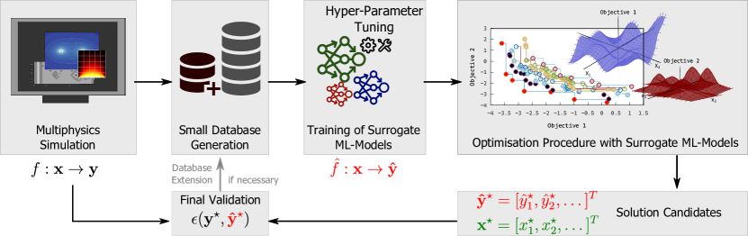
Figure 1: Proposed strategy for training and self-optimizing surrogate models using machine learning and deep learning techniques to tackle multiobjective optimization problems in complex multiphysics approaches.

To address the issue of high computational demand and time-consuming optimization procedure, we propose using surrogate models, i.e. data-driven algorithms, as an alternative to running computationally expensive multiphysics simulations. Some optimization algorithms, like optimization via gradient descent, require the queried models to be fully differentiable. By using adequate surrogate models, it becomes possible to apply such optimization algorithms to non-differentiable multiphysics systems. As shown in Fig. 1, our strategy can be summarised as follows: First, we identify the multiphysics system input and output space followed by a small data generation procedure. Next, we apply our pipeline for the training and evaluation of machine learning (ML) models, which are then used for the optimization task of the input parameters of the multiphysics system. Finally, we validate the optimization results by comparing the outputs of the ML models against the simulated values of parameter combinations, which correspond to solution candidates of the multi-objective optimization problem. The potential of surrogate models in multiphysics simulations is vast, as they can help reduce the computational burden of running full-scale simulations. This, in turn, can speed up the design and optimization process, reduce the cost of simulations, and enable researchers to explore a broader range of design options. The main contributions of our paper can be summarized as follows:

1. Two real-world tabular datasets using multiphysics simulations, which are made publicly available

2. Compared to other deep learning applications, we show that surrogate models can be trained on relatively small amounts of data to approximate those simulations accurately

3. We conduct extensive experiments combining four different surrogate models with two optimization algorithms to solve two challenging real-world multiobjective optimization problems

4. We evaluate the performance of our combined training and optimization pipeline by verifying the final Pareto-optimal results using the ground truth multiphysics simulations

5. We derive insights about the relevance of features in our real-world examples by examining our surrogates using explainable AI techniques

The remainder of this article is structured as follows: Section II summarizes the related work, followed by a presentation of our combined training and optimization pipeline in Section III, where we also explain the main components in detail. Section IV describes the underlying physical problems of the two real-world tabular datasets used in our approach. The results of our evaluation strategy for training and optimization with an examination of the acquired results with explainable AI methods are presented in Section V. Finally, Section LABEL:sec:conclusion summarizes the main conclusions and open issues for future work.

II Related Work

The availability of increased computational power has facilitated advanced multiphysics simulations, allowing the coupling of diverse physical phenomena. However, challenges associated with the coupling process may limit stability, accuracy, and robustness [1, 2]. In recent years, there has been a significant increase in research focused on leveraging ML techniques to enhance the capabilities of multiphysics problems and address associated challenges. The potential for optimizing computational fluid dynamics (CFD) conjugate heat transfer systems using deep reinforcement learning has been investigated [3], underlining the optimization task in large parameter spaces and discovering unexpected solutions. In our paper, the task of finding optimal solutions for multiphysics problems under challenging constraints is divided into two parts: the training of surrogate models that generalize accurately and the subsequent optimization of those surrogates.

II-A Surrogate models for multiphysics problems

[4] showcase an autoencoder architecture to model the scalar transport equation in a coupled system of Navier-Stokes equations and heat energy equation for simulating forced convection cooling However, features learned by autoencoders are difficult to interpret or explain. Neural Operators [5] can be used to solve challenging multiphysics-problems. Those operators often times require specialized architectures and large amounts of training data.

Physics-informed neural networks (PINNs) [6, 7, 8] are a powerful tool to obtain solutions for multiphysics simulations without access to ground-truth data. However, PINNs require substantial physics knowledge and careful incorporation to avoid overfitting, making them less accessible to non-experts. Additionally, PINNs can be computationally expensive and time-consuming to train, needing significant resources to converge to accurate solutions.

In contrast to previous works, we parametrize the multiphysics problem in tabular form, which makes it possible to directly apply standard machine learning methods for training surrogates on tabular data and develop optimization algorithms on top of those.

II-B Multiphysics optimization and data extension

Limited data poses significant challenges in multiphysics simulations, and only a few works highlight the challenges in specific use cases. A data-driven approach to compute approximate solutions for the induction hardening (IH) process shows promising results and provides good approximations in the low-data limit case [9]. Another approach uses a deep generative design framework that integrates topology optimization and generative models (e.g., generative adversarial networks (GANs)). It allows the exploration of new design options, thus generating many designs starting from limited previous design data. In addition, anomaly detection evaluates the novelty of generated designs, thus helping designers choose among design options and reducing the number of simulations [10]. In a preliminary investigation of one of our use cases, we explored the applicability of novelty and anomaly detection algorithms in design optimization tasks. The study found that these algorithms are effective in exploring the design space, but they have limitations when it comes to exploitation [11].

Multiobjective optimization requires to find trade-offs between potentially conflicting objectives [12], which quickly becomes a challenging task for automated optimization algorithms. [13] investigate this problem through the lens of diversity and are able to show that their approach is able to increase diversity without sacrificing global performance.

In our work, we shift the decision to weigh the different objectives to the user by presenting a range of pareto-fronts of optimized designs. We additionally encourage diversity of our optimized results by carefully choosing our optimization algorithms.

III ML Supported optimization Strategy

Our study presents an innovative strategy for training and self-optimising surrogate models, particularly machine learning and deep learning techniques. These models can be integrated into the optimization process of multiphysics problems, which is a notoriously challenging task. Our approach, depicted in Fig. 2, consists of three main blocks, which we will explain in the following.

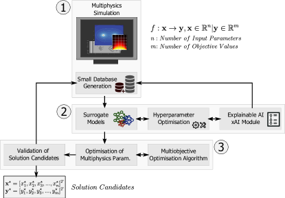
Figure 2: Illustration of our proposed Pipeline for self-optimising surrogate models, which can be seamlessly integrated into the optimization process of multiphysics problems and comprises three main blocks: data acquisition, surrogate model training, and multiobjective optimization.

III-A Data Acquisition

The first block (1) consists of the data acquisition module, which generates a small database using simulation results from available numerical models. This step poses significant challenges, as the generation process must satisfy specific requirements, including providing high diversity of the input features’ parameter range and sufficient information for training the surrogate models.

Several factors must be considered in the proposed pipeline, including the complexity of the models, which can impede the acquisition of large amounts of data due to the high number of parameters and increased dimensionality. Additionally, incomplete or noisy data can result from measurement errors or numerical inaccuracies during the simulation process, which can impact the accuracy and reliability of the machine-learning models. Another challenge is the lack of standardization in multiphysics simulations, as there can be significant variations in the physical models, numerical methods, and simulation parameters used. This lack of standardization makes it difficult to compare results from different simulations and to develop generalizable machine learning and deep learning models.

III-B Surrogate Models

Next, surrogate models are trained on the generated datasets, as shown in block 2. We employ multiple methods and hyperparameter optimization strategies to ensure robust training of the models. To identify possible unexplored areas that should be generated in the first block, it is crucial to understand the dependencies present in the data. To achieve this, our approach incorporates explainable artificial intelligence (xAI) techniques that provide insights into the relevant feature dependencies. By analyzing the results obtained from xAI methods, we can identify areas in the data that have not been fully explored and extend the database accordingly.

In our pipeline, we employ multiple methods to predict target values in the multiphysics process. As a baseline, we train XGB surrogate models, which provide valuable insights into the underlying problem and data dependencies. For each target value, we train a single XGB Regressor and optimise each model’s hyperparameters independently using a combined cross-validation and Bayesian optimization strategy.

In addition to the XGB surrogate models, we employ ensemble strategies combining multiple scikit-learn regressors at the decision level [autosk]. A two-step process to train and optimize the hyperparameters consists of first performing a random search of hyperparameters to identify promising regressors. Then, we combine these regressors into an ensemble using a weighted average, where the weights are learned through gradient-based optimization. The ensemble is trained using cross-validation, and we select the best-performing ensemble based on validation scores. The final ensemble is trained on the entire dataset and used for prediction. This approach balances exploring the hyperparameter space and exploiting the most promising models.

Finally, we explore two deep-learning techniques, MLP and CNN, for the regression task. We use both models to estimate all target values, and we tune the hyperparameters of each model using a combined cross-validation and Bayesian optimization strategy. In this study, we focus on evaluating the regression performance using deterministic metrics, but we acknowledge the need to consider non-deterministic approaches in future work.

III-C Interpretable Surrogate Modelling

It is crucial to interpret the results to ensure that ML-supported multiphysics simulations perform optimally. This can be challenging when dealing with sparse data or inadequate surrogate models. However, using a highly interpretable machine learning model can help individuals understand the model’s predictions and decisions. We leveraged the XGB regressor as our baseline and used feature relevances to better understand the impact of input features on target values.

Furthermore, we extended our approach using partial dependence plots (PDP) to identify whether the relationship between relevant features and target values is linear, non-linear, monotonic, or more complex. PDP is a powerful technique that shows the marginal effect of one or two variables on the predicted outcome of a machine learning model while holding all other variables constant. While we used these specific techniques in our study, different approaches, such as feature importance, local interpretability, and rule-based models, can be employed to enhance the interpretability of machine learning models.

III-D Optimization

The third block (3) of our approach leverages the pre-trained machine learning models to perform the multi-objective optimization task. It employs a diverse set of optimization approaches, including evolutionary algorithms, gradient-based techniques, and random search, to generate solution candidates for the underlying optimization task. A validation step is required to validate the performance of the surrogate models and the generated solution candidates. If the results obtained from this step exhibit high error values against numerical simulations, the database may need to be extended, and the pipeline must be rerun.

The first optimization algorithm is a non-dominated sorting genetic algorithm (NSGA). Genetic algorithms have proven to be a robust and reliable design optimization method [14]. Therefore, we integrated the NSGA-2 into our optimization pipeline [15].

As a second optimization algorithm we use gradient-based optimization in the input feature space directly. For the fully-differentiable models (CNN, MLP), we freeze the parameters of the model and perform gradient update steps in the input space. We scale all target quantities to $[0,1]$ before computing the loss function to ensure equal weighting of the loss terms using the following scaler function:

$$\lambda(x)=\frac{x-\min(X)}{\max(X)-\min(X)}$$ (1)

where $x$ is an individual data point, $\min(X)$ and $\max(X)$ represent the minimum and maximum values in the train dataset, respectively. We then optimize the following loss functions for the Motor and U-bend problem respectively:

$$\mathcal{L}_{motor}=-\alpha\lambda(J_{M})+\beta\lambda(J_{m})+\gamma\lambda(J_{\Phi})$$ (2)

$$\mathcal{L}_{U-Bend}=\alpha\lambda(J_{p})+\beta\lambda(J_{T})$$ (3)

For the motor problem $J_{M}$ denotes the normalized torque, $J_{m}$ is the normalized magnet mass and $J_{\Phi}$ is the normalized total loss. For the cfd problem, $J_{T}$ denotes the cooling power and $J_{p}$ the pressure loss.

To generate diverse solutions along the Pareto-front, we start gradient-based optimization from 1000 randomly selected combinations of input features. Each input feature is sampled individually from a uniform distribution over the range of training features. For each 1000 runs of gradient-based optimization, we uniformly sample $\alpha,\beta$ [and $\gamma$] in the $[0,1]$ range to cover the Pareto-front even better.

IV Experimental Design

IV-A Use Case 1: Motor Dataset

In this section, the baseline machine considered for optimization is described in terms of its dimensions/parameters, constraints, and performance characteristics. For this paper, a 60-slot 10-pole Internal Permanent Magnet Synchronous machine is considered and is to be optimized for average torque, total loss and magnet mass. As shown in figure 3, there are two lateral magnets (Magnet1-big, Magnet2-small) embedded into the rotor iron sheets. In addition, two air cavities (air cavity1-big, air cavity2-small) are designed in the rotor topology to guide the magnetic fluxes from the magnets into the air gap at the stator-rotor interface. For this work, only the rotor topology of the baseline machine is parameterized with 15 geometric parameters namely - height of magnet1 hi_mag1, width of magnet1 wi_mag1, radial distance of magnet1 from origin r_mag1, height of magnet2 hi_mag2, width of magnet2 wi_mag2, radial distance of magnet2 from origin r_mag2, height of air cavity1 hi_ac1, width of air cavity1 wi_ac1, distance between air cavity1 and rotor dist_ac1_rot, a length of a segment defining air cavity1 dist2_ac1, another length of a segment defining air cavity1 dist3_ac1, x coordinate of center defining air cavity2 x_ac2, y coordinate of center defining air cavity2 y_ac2, width of air cavity2 wi_ac2, and height of air cavity2 hi_ac2. Since, these 15 parameters have a significant impact on the average torque, losses and magnet mass, they have been selected as design variables for the optimization problem.

Fig. 3 presents a segment of the baseline machine’s rotor topology in 2D along with the design variables considered for optimization.

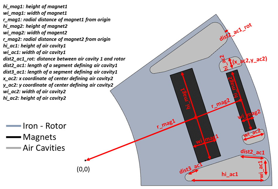
Figure 3: Parameterized 2D rotor segment of the baseline machine

Through these 15 parameters, the size as well as the position of the magnets and air cavities of the baseline machine can be varied using Design of Experiments (DOE) techniques to generate rotor topology variants. Different methods of DOE are available to efficiently explore the design space with minimal number of sampling points for FE-simulations. For instance, orthogonal array (OA) based sampling is used in  [16] to reduce the computational effort. Similarly, a fractional factorial based Box-Behnken method is employed in  [17] in contrast to full-factorial approach to reduce the number of sample points.  [18] used stratification based Latin Hypercube Design (LHD) for performing DOE. In this work, an advanced version of LHD called Optimal Latin Hypercube Design (OLHD) is employed to get an excellent space filling with limited sampling points. The Uncertainty Quantification module of COMSOL 6.0 is used to generate 1000 samples points using OLHD algorithm. A methodology to check for the plausibility of the generated geometric variants and to automate the process of FE-Model buildup and simulation of multiple machines in a loop was developed internally. For this work, about 800 plausible variants were simulated for one working point in COMSOL and the simulation results are evaluated using MATLAB. Further, a methodology to save the design parameters and target values for each variant into an Excel Sheet was developed. This way the generation of simulation database for AI Modelling is sustainably accelerated and in addition, it facilitates the ease of using the database for building AI models.

Table II presents the dimensions/parameters, constraints, and performance characteristics the baseline machine.

TABLE I: Dimensions/Parameters, Constraints, and Performance Characteristics

Dimension/Parameter	Value
Stator outer Diameter	230 [mm]
Rotor outer Diameter	152 [mm]
Airgap Length	1 [mm]
Magnet Remanence	1.18 [T] at 120 $\tccentigrade$
Constraint	Value
Maximum allowable Current	636.34 [A]
Maximum allowable Voltage	270 [V]
Performance Characteristic	Value
$J_{M}$ Torque @1000 rpm	280.5 [Nm]
$J_{\Phi}$ Total Losses @1000 rpm	3.76 [kW]
$J_{m}$ Magnet Mass	2.78 [kg]

As described in III-D, goals of the optimization problem are to maximize the average torque ($J_{M}$) while simultaneously minimizing the total loss ($J_{\Phi}$) and magnet mass ($J_{m}$). Therefore, the optimization goals are conflicting in nature. The average torque mainly depends on the flux density at the air gap interface between stator and rotor. For a constant length of the machine, the average torque can be increased using larger magnets, however the costs associated with expensive magnet material increases. In addition, the size and shape of the air cavities have a significant effect on the average torque delivered by the machine. Similarly, the radial position of the magnets affects the flux distribution and therefore the average torque. All the changes made to size, position and shape of the magnets and air cavities will in turn alter the amount of soft iron used for rotor segments and therefore the associated iron loss. This makes the optimization problem complex and therefore efficient algorithms are needed to find a global optimum. The output of such a multi-objective optimization problem with conflicting objectives is a Pareto front with several optimal solutions. From this Pareto front, a design, which best satisfies all the three goals will be selected. Fig. 4 presents a distribution of the three optimization goals or targets used for training and testing.

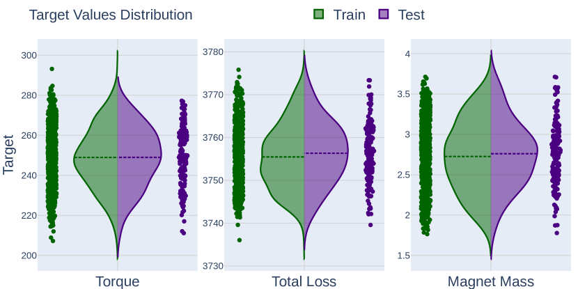
Figure 4: Target Values Distribution Case 1

IV-B Use Case 2: U-Bend Dataset

The second use case is from the field of fluid dynamics. Flow deflections are a prevalent reason for energy dissipation in technical systems. Typical applications include large-scale piping grids or cooling channels of gas turbine blades, for example. The dataset is freely available and described in detail [19], therefore, we will focus on the main features in the following. In Figure 5 a single design can be seen. It is described by 28 design-parameters consisting of 6 boundary points, depicted in green and 16 curve parameters, depicted in red. The 6 boundary points can vary on the x and on the y-axis, therefore, they have 2 degrees of freedom each. The boundary points of the outer layer (o) vary in a parameter range between -1 and 1. On the inner layer (i) the boundary point of levels C and E can vary between -1 and 1 on the y-axis. Boundary point Di varies in a range of -1 to 1 on the x and 0 to 1 on the y-axis. The 16 curve parameters are within a range of 0 to 1. A value of 0 indicates that the curve parameter is located on the boundary parameter of its origin, whereas a value of 1 indicates that it is located on the opposite boundary parameter. The origin is indicated by the blue line. Overall, the U-bend design is characterized by a relatively large number of parameters and significant degrees of freedom, which offers considerable flexibility in its design and potential for optimization. The hydraulic diameter $d_{h}$ is set to 0.0075m.

[mode=image]images/ubend_case

Figure 5: Parameterized geometry with boundary points (green) and curve parameters (red). Figure is adapted from [11]

With the help of Computational Fluid Dynamics methods the two target values $J_{p}$ for $pressure\_loss$ and $J_{T}$ $cooling\_power$ are determined. The Navier-Stokes equations determine the velocities of the fluid and the pressure. In addition, the energy equation is used to consider the heat conduction and the convective heat transfer between fluid and solid using a multi-physics solver. The cooling capacity is defined inversely. A small value for this target value indicates a high cooling power. Both targets conflict with each other, therefore, no design minimizes both targets; hence a classical multi-objective optimization problem is present.
We use a subset of the available data, furthermore, we restrict ourselves exclusively to the parameter representation of the dataset [19] to ensure comparability with use case 1. The training dataset includes 800 and the test dataset includes 200 designs.

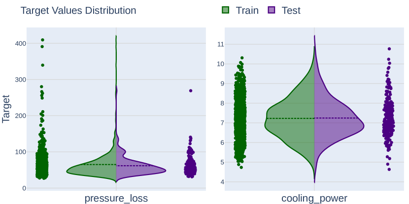
Figure 6: Target Values Distribution Case 2

V Results

We aim to demonstrate the versatility of our pipeline for different multiphysics problems by employing a comprehensive and consistent evaluation strategy. To this end, we structure our results and subsequent subsections as follows: Subsection V-A showcases the performance of the involved ML-surrogate models in the regression task. Subsection V-B provides valuable insights into the regression task’s outcomes. An evaluation and discussion of the results obtained with two different optimisation strategies are presented in subsection V-C. Moreover, in Subsection V-D, we validate the acquired solution candidates by comparing the predictions of the surrogate models against the numerical simulations.

V-A Regression Performance

To compare and interpret the results obtained after the training process of the surrogate models for the prediction of the target values described in Section IV, we use the Mean Absolute Percentage Error (MAPE) as a commonly used deterministic regression metric. MAPE allows evaluating the models’ performance regardless of the target’s scale but has some limitations. For example, it is sensitive to extreme or zero values (division by zero) and can be heavily influenced by outliers. For this reason, the inspection of additional scores is always recommended, and the evaluation of the regression performance with additional metrics for the presented use cases is provided in Appendix II.

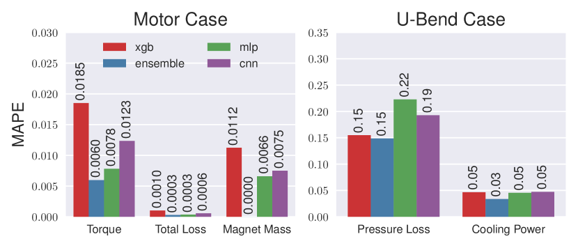
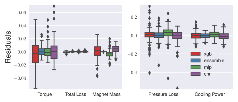
Figure 7: Assessing Surrogate Performance: MAPE and Residual Analysis on Test Dataset for each Use Case

In Fig. 7 using the bar plots, we present the evaluation results of four different surrogate models based on the test dataset (20%). We observe that the models exhibit superior performance in predicting motor performance on the Motor dataset, with MAPE values below 1.9%. On the other hand, the U-Bend dataset represents a more challenging task, as indicated by the higher MAPE values of approximately 22% for an MLP surrogate-model when predicting the Pressure Loss. However, despite the difficulty of the U-Bend dataset, the models demonstrate better performance in predicting the second target variable, Cooling Power, with MAPE values below 5%. Fig. 7 (Residual Boxplots) highlights the presence of high residual values for particular data points in predicting Pressure Loss specifically for the U-Bend dataset. These outliers may contribute to the elevated MAPE values observed for the same target variable, as the MAPE metric is sensitive to such extreme values. In contrast, the Motor dataset exhibits significantly lower residual values when compared to the U-Bend case.

Another potential explanation for the comparatively imprecise prediction error in U-Bend Case as compared to Motor Case is the greater dimensionality of the input space, which amounts to 28 dimensions as opposed to the Motor Case with 15 dimensions. As described in sections IV-A and  IV-B, the target values are not normally distributed. Utilizing the mean squared error (MSE) metric during optimization leads to a particularly severe penalty for outliers. Consequently, the optimization process becomes more challenging in regions featuring low target values, as they have less weight when squared. Additionally, in U-Bend Case, the flow is entirely turbulent, meaning that even the slightest change to the parameter space could result in vortex generation and, consequently, discontinuities in the objective function. Furthermore, the underlying physics of the two cases differ significantly. Specifically, while the Maxwell equation represents a first-order linear partial differential equation, the Navier-Stokes equation represents a system of second-order nonlinear partial differential equations featuring five solution variables. These fundamental differences in the mathematical formulations of the problem could contribute to disparities in the precision of the predictive outcomes between the two use cases.

Our training strategy demonstrates excellent performance in predicting the target values for both cases. Among the various approaches we employed, the ensemble strategy consistently outperforms the others. Moving forward, we delve deeper into the regression task and explore the dependencies between features and target values. This exploration is facilitated by applying explainable artificial intelligence (xAI) techniques, which allow us to gain valuable insights into the underlying relationships. The next part of our evaluation strategy focuses on leveraging these xAI techniques to provide further analysis and understanding.

V-B Identifying Critical Features and relevant dependencies

Interpreting the obtained results with the different algorithms is crucial to provide insights into the regression task defined for predicting the target values. First, we consider the evaluation of feature importances of each XGB model trained independently for the prediction of a single target value. In the Motor case, we have three XGB models for the prediction of each target value, e.g. Torque, Total Loss and Magnet Mass. For the U-Bend dataset, we evaluate two XGB models for the target values Pressure Loss and Cooling Power. The corresponding importance values are shown in Fig. 8. In the Motor case, we observe a high dependency of the Magnet Mass from the input feature wi_mag1, which is the main reason for the weaker performance compared to the other models, cf. Fig. 7. As described in Section IV-A. There is more than one parameter influencing the size of the lateral magnets. Therefore, the XGB model emphasizes only one feature for predicting the Magnet Mass. The feature with high importance may exhibit a strong nonlinear relationship with the target variable, while other features have relatively weaker relationships. In such cases, the model emphasizes the feature with the stronger nonlinear impact and assigns it higher importance.

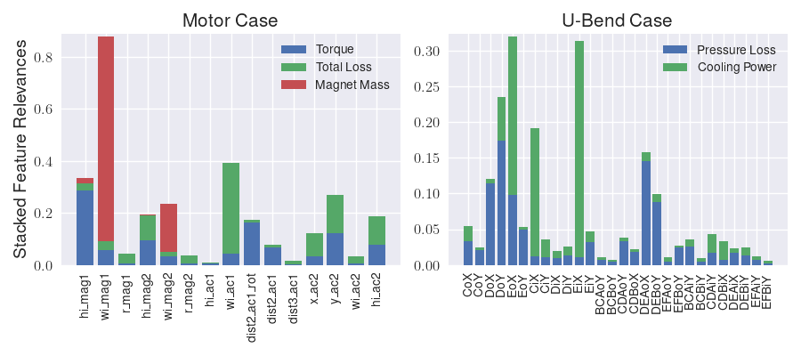
Figure 8: Feature Importance Analysis: Stacked Relevancies of XGBoost Models for Target Value Prediction in Each Use Case

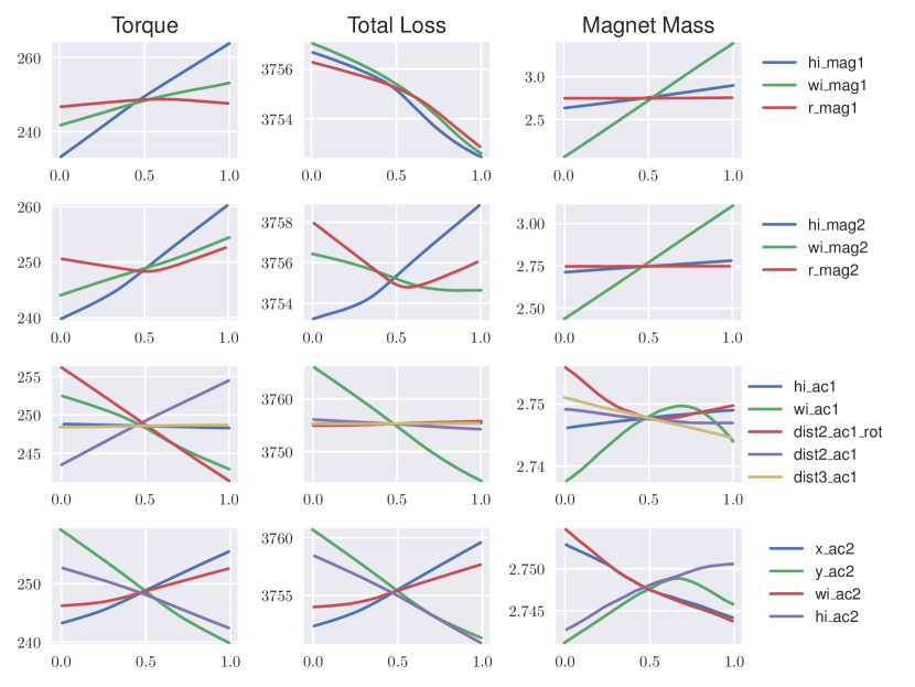
Figure 9: Feature dependencies in the prediction of target values for the Motor dataset

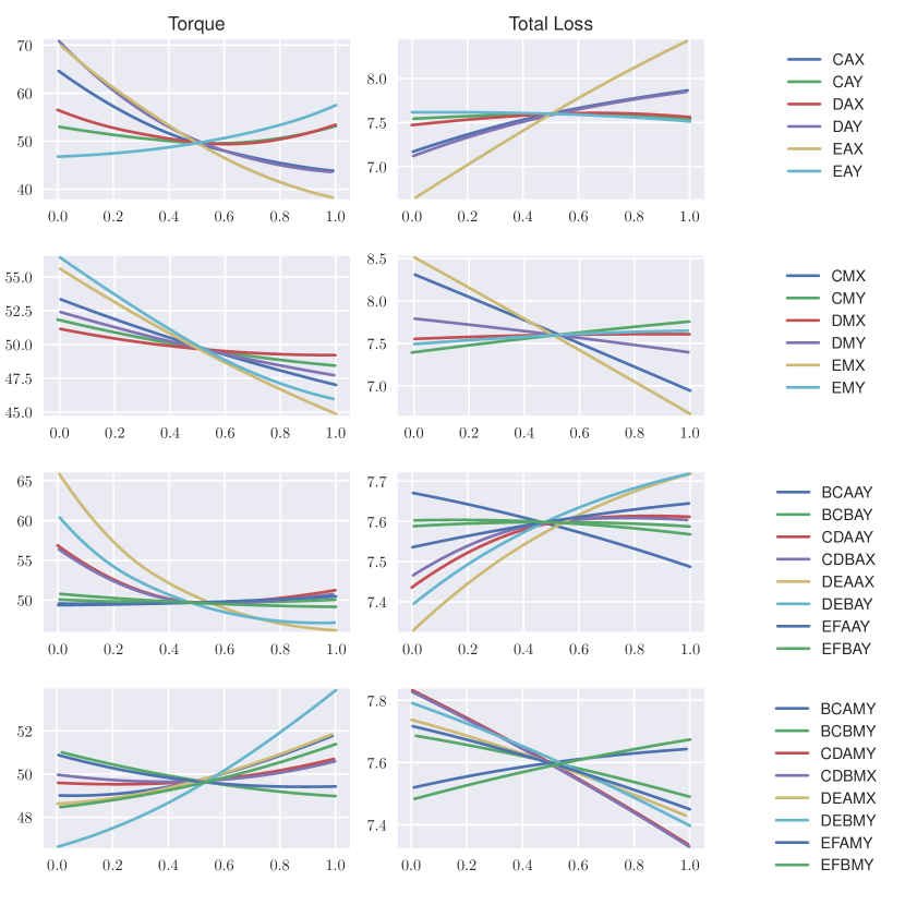
Figure 10: Feature dependencies in the prediction of target values for the U-Bend Use Case

In discussing the results obtained from the Explainability Module for the U-Bend Case, one notable strength of the problem becomes apparent. Despite its high complexity, the problem can be interpreted physically from a fluid dynamic perspective, enabling the verification of results derived from the Explainability Module. Let us examine the principal factors influencing the Pressure Loss. The parameter known as DoY controls the width of the channel on the outer layer at the deflection point along the Y-axis. From a physical standpoint, this relationship is sensible as widening or narrowing the channel cross-section leads to a decrease or increase in the local Reynolds number, respectively. A higher Reynolds number indicates greater turbulence, which promotes vortex formation and significantly contributes to the Pressure Loss. The same argumentation is applicable for the parameter EoX, but it is understandable that this parameter has a smaller influence. In addition, it is plausible that the outer curve parameters have a stronger influence on the Pressure Loss, as the flow should be adjacent in particular in its wake to prevent vortex formation. Too small curve parameters, however, would lead to excessive deflection, which would result in a stall.

When examining the target value of the Cooling Power, it becomes evident that the parameters EoX, CiX, and EiX play a significant role as influencing factors. This outcome aligns with expectations, particularly considering that the parameters associated with the inner layer have a direct correlation with the heated surface. A thinner solid surface implies reduced resistance to heat conduction. At the prevailing high Reynolds numbers, convective heat transfer from the solid to the fluid is the dominant mechanism, rendering the heat conduction resistance attributable to a thin solid preferable. In this context, promoting contact flow remains desirable, but an enhancement in cooling performance would result from channel narrowing, primarily controlled by the outer parameters.

V-C Evaluation of Solution Candidates in the Multiobjective optimization Task

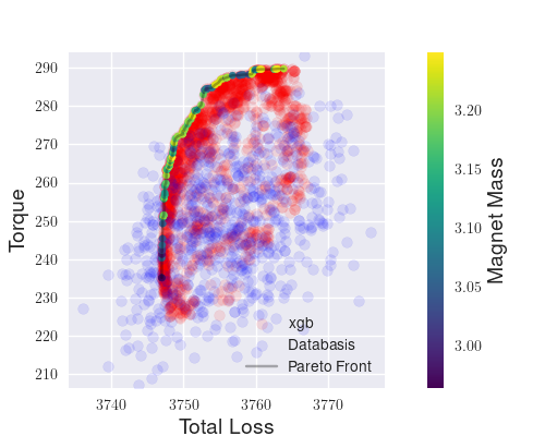
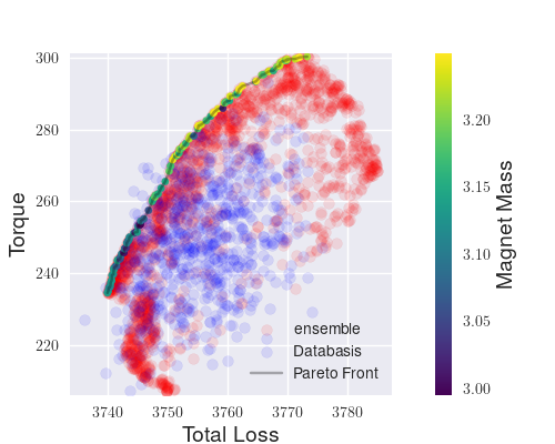
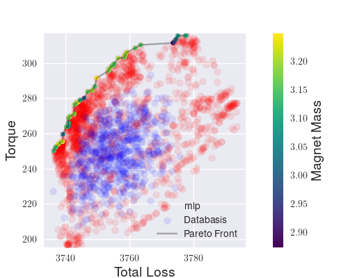
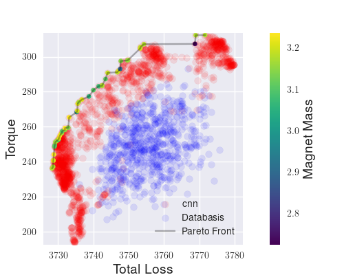
Figure 11: Optimisation Results for the Motor Use Case with EA in combination of four different surrogate models

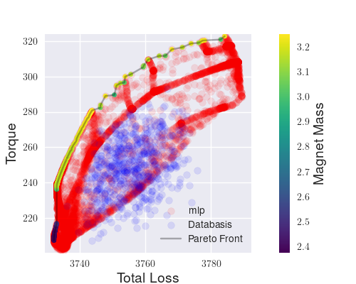
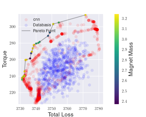
Figure 12: Optimisation Results for the Motor Use Case with a Gradient-Based Optimisation Strategy in combination of two surrogate models

In the U-Bend Use Case, a two-dimensional Pareto frontier is sufficient due to the presence of only two objective values. As shown in Figure 14, each model generates a Pareto frontier when evolutionary optimisation is applied. These frontiers offer design candidates that outperform those in the original database, depicted as blue dots.

However, upon closer examination, an issue arises. Three out of the four models forecast negative pressure loss values. A zero or negative pressure loss is physically unrealistic, as it would imply that no energy is needed to move the fluid through the cooling channel. This suggests that these models may not have completely captured the underlying physical principles.

Further analysis, involving the recalculation of the proposed design candidates from these Pareto frontiers, will help quantify the extent to which these models are accurate or flawed.

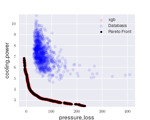
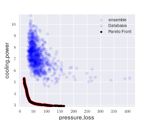
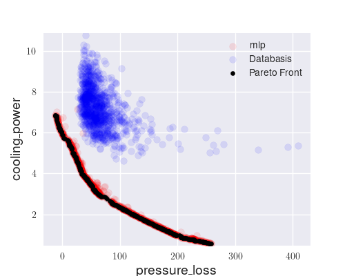
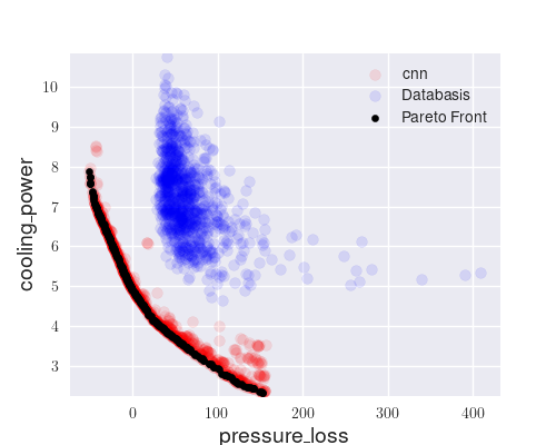
Figure 13: Optimisation Results for the CFD Use Case with EA in combination of four different surrogate models

As in Figure 14 can be seen, it is evident that the gradient-based optimisation strategies under consideration perform suboptimally for the U-Ben Use Case. Both the MLP and the CNN models yield Pareto frontiers that are inferior to the original data set in a large range of the target space. Consequently, these Pareto frontiers lack plausibility, suggesting a failure in the optimisation process.

The underlying cause of this phenomenon is likely the high dimensionality of the design space, which is characterised by 28 design parameters. It is a plausible supposition that the gradient-based optimisation methods are entrapped in local minima, unable to extricate themselves towards either superior local minima or the global minimum.

While the limitations of the gradient-based optimisation strategy are evident, one notable advantage emerges analising the 13 and 14. Examining the Pareto frontier generated by both models, it is reassuring to note the absence of implausible design candidates. Specifically, the models did not predict any design configurations yielding unrealistically favourable target values, such as pressure losses below zero. This suggests that, despite their shortcomings in optimisation, the models remain grounded in a level of realism, refraining from predicting physically impossible scenarios

In contrast, when utilising evolutionary optimisation methods with the identical models, we observe a significant improvement in the quality of the resulting Pareto frontiers. This lends credence to the notion that the limitations are not intrinsic to the models themselves, but rather arise from the gradient-based optimisation process employed. Therefore, we can reasonably conclude that gradient-based optimisation is the limiting factor in this complex high-dimensional space.

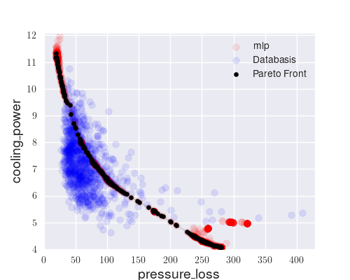
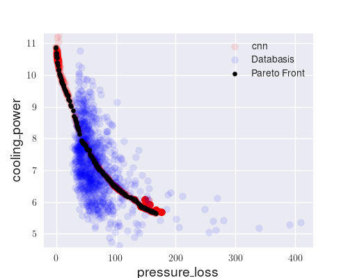
Figure 14: Optimisation Results for the CFD Use Case with a Gradient-Based Optimisation Strategy in combination of two surrogate models

V-D Validation of Solution Candidates in the Multiobjective optimization

In the last stage of our evaluation strategy we examine the predition accuracy of our surrogates for the solution candidates. We show the distribution of the optimized target quantities vs. the training distribution in the appendix.

Figure 15: MAPE of the final validation for Motor Use Case

We show the MAPE score of our optimization results compared to the validated results from the ground truth simulation in figure 15.

Figure 16: MAPE of the final validation for dataset cfd

We show the MAPE score of our optimization results compared to the validated results from the ground truth simulation in figure 16. In recalculating a subset of the pareto optimal design samples with CFD-simulations, we find that the cooling power predictions are more accurate than those for pressure loss. This matches well with the discussion earlier.

It’s also important to note that the overall MAPE, is higher in the U-Bend Use Case compared to the Motor Use Case. This was expected, due to the U-Bend’s more complex design space and more challenging physical principles

Appendix A

TABLE II: Design Variables and their ranges

Design Variable	Range
hi_mag1	[21.4, 24.3] mm
wi_mag1	[4, 8] mm
r_mag1	[15, 19] mm
hi_mag2	[14.6, 16.2] mm
wi_mag2	[2, 5] mm
r_mag2	[28.5, 30.5] mm
hi_ac1	[18, 20] mm
wi_ac1	[1.8, 3.3] mm
dist2_ac1_rot	[0.6, 1.6] mm
dist2_ac1	[4.2, 6.2] mm
dist3_ac1	[1.5, 3.5] mm
x_ac2	[68.4, 69.2] mm
y_ac2	[8.4, 9.1] mm
wi_ac2	[5.4, 6.2] mm
hi_ac2	[2.5, 3.2] mm

TABLE III: Regression Performance on a tabular test dataset of a baseline electric traction machine

Target	Magnet Mass				Torque				Total Loss
	xgb	ensemble	mlp	cnn	xgb	ensemble	mlp	cnn	xgb	ensemble	mlp	cnn
r2	0.991	1.000	0.997	0.997	0.852	0.984	0.968	0.922	0.560	0.964	0.941	0.855
nrmse	0.096	0.000	0.055	0.059	0.383	0.126	0.177	0.279	0.661	0.189	0.241	0.379
nmse	0.009	0.000	0.003	0.003	0.147	0.016	0.031	0.078	0.437	0.036	0.058	0.144
mse	0.002	0.000	0.001	0.001	32.650	3.540	6.989	17.319	23.197	1.903	3.093	7.626
nmae	0.011	0.000	0.007	0.007	0.018	0.006	0.008	0.012	0.001	0.000	0.000	0.001
mae	0.031	0.000	0.018	0.020	4.578	1.474	1.926	3.056	3.837	1.095	1.314	2.131
nbias	0.001	0.000	-0.005	0.005	-0.002	0.000	0.000	0.001	-0.001	0.000	-0.000	0.000
mape	0.011	0.000	0.007	0.007	0.019	0.006	0.008	0.012	0.001	0.000	0.000	0.001
rmse	0.040	0.000	0.023	0.024	5.714	1.881	2.644	4.162	4.816	1.379	1.759	2.762
bias	0.002	0.000	-0.013	0.014	-0.576	0.047	0.096	0.331	-3.202	0.015	-0.098	0.008

TABLE IV: Regression Performance on CFD Dataset

Target	cooling Power				Pressure Loss
	xgb	ensemble	mlp	cnn	xgb	ensemble	mlp	cnn
r2	0.813	0.907	0.835	0.803	0.537	0.727	0.501	0.459
nrmse	0.431	0.304	0.405	0.443	0.679	0.521	0.705	0.733
nmse	0.186	0.092	0.164	0.196	0.461	0.272	0.496	0.538
mse	0.185	0.092	0.163	0.195	316.363	186.636	340.679	369.199
nmae	0.046	0.034	0.045	0.048	0.168	0.151	0.216	0.200
mae	0.334	0.243	0.325	0.346	10.368	9.321	13.330	12.313
nbias	-0.005	-0.006	0.012	-0.013	0.023	0.008	0.111	-0.035
mape	0.047	0.034	0.045	0.047	0.155	0.149	0.223	0.193
rmse	0.430	0.304	0.404	0.442	17.787	13.661	18.457	19.215
bias	-0.038	-0.041	0.090	-0.092	1.423	0.487	6.831	-2.137

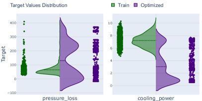
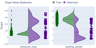
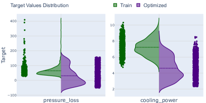
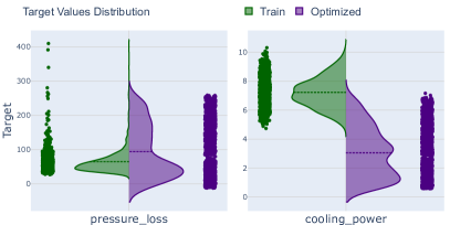
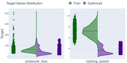
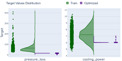
Figure 17: Violin plots depicting the train distribution of targets vs. the distribution of targets for the optimisation results for the cfd dataset.

References

- [1] D. Groen, S. J. Zasada, and P. V. Coveney, “Survey of Multiscale and Multiphysics Applications and Communities,” Computing in Science & Engineering, vol. 16, no. 2, pp. 34–43, Mar. 2014, conference Name: Computing in Science & Engineering.
- [2] D. E. Keyes, L. C. McInnes, C. Woodward, W. Gropp, E. Myra, M. Pernice, J. Bell, J. Brown, A. Clo, J. Connors, E. Constantinescu, D. Estep, K. Evans, C. Farhat, A. Hakim, G. Hammond, G. Hansen, J. Hill, T. Isaac, X. Jiao, K. Jordan, D. Kaushik, E. Kaxiras, A. Koniges, K. Lee, A. Lott, Q. Lu, J. Magerlein, R. Maxwell, M. McCourt, M. Mehl, R. Pawlowski, A. P. Randles, D. Reynolds, B. Rivière, U. Rüde, T. Scheibe, J. Shadid, B. Sheehan, M. Shephard, A. Siegel, B. Smith, X. Tang, C. Wilson, and B. Wohlmuth, “Multiphysics simulations: Challenges and opportunities,” The International Journal of High Performance Computing Applications, vol. 27, no. 1, pp. 4–83, Feb. 2013, publisher: SAGE Publications Ltd STM.
- [3] E. Hachem, H. Ghraieb, J. Viquerat, A. Larcher, and P. Meliga, “Deep reinforcement learning for the control of conjugate heat transfer,” Journal of Computational Physics, vol. 436, p. 110317, Jul. 2021.
- [4] G. El Haber, J. Viquerat, A. Larcher, D. Ryckelynck, J. Alves, A. Patil, and E. Hachem, “Deep learning model to assist multiphysics conjugate problems,” Physics of Fluids, vol. 34, no. 1, p. 015131, Jan. 2022.
- [5] N. Kovachki, Z. Li, B. Liu, K. Azizzadenesheli, K. Bhattacharya, A. Stuart, and A. Anandkumar, “Neural operator: Learning maps between function spaces with applications to pdes,” Journal of Machine Learning Research, vol. 24, no. 89, pp. 1–97, 2023. [Online]. Available: http://jmlr.org/papers/v24/21-1524.html
- [6] P. Sharma, W. T. Chung, B. Akoush, and M. Ihme, “A Review of Physics-Informed Machine Learning in Fluid Mechanics,” Energies, vol. 16, no. 5, p. 2343, Jan. 2023, number: 5 Publisher: Multidisciplinary Digital Publishing Institute.
- [7] M. Raissi, P. Perdikaris, and G. E. Karniadakis, “Physics-informed neural networks: A deep learning framework for solving forward and inverse problems involving nonlinear partial differential equations,” Journal of Computational Physics, vol. 378, pp. 686–707, Feb. 2019.
- [8] G. E. Karniadakis, I. G. Kevrekidis, L. Lu, P. Perdikaris, S. Wang, and L. Yang, “Physics-informed machine learning,” Nature Reviews Physics, vol. 3, no. 6, pp. 422–440, Jun. 2021, number: 6 Publisher: Nature Publishing Group.
- [9] K. Derouiche, S. Garois, V. Champaney, M. Daoud, K. Traidi, and F. Chinesta, “Data-Driven Modeling for Multiphysics Parametrized Problems-Application to Induction Hardening Process,” Metals, vol. 11, no. 5, p. 738, 2021.
- [10] S. Oh, Y. Jung, S. Kim, I. Lee, and N. Kang, “Deep Generative Design: Integration of Topology Optimization and Generative Models,” Journal of Mechanical Design, vol. 141, no. 11, 2019.
- [11] J. Decke, J. Schmeißing, D. Botache, M. Bieshaar, B. Sick, and C. Gruhl, “Ndnet: A unified framework for anomaly and novelty detection,” in Architecture of Computing Systems, M. Schulz, C. Trinitis, N. Papadopoulou, and T. Pionteck, Eds. Cham: Springer International Publishing, 2022, pp. 197–210.
- [12] O. Sener and V. Koltun, “Multi-task learning as multi-objective optimization,” Advances in neural information processing systems, vol. 31, 2018.
- [13] T. Pierrot, G. Richard, K. Beguir, and A. Cully, “Multi-objective quality diversity optimization,” in Proceedings of the Genetic and Evolutionary Computation Conference, 2022, pp. 139–147.
- [14] M. Choi, G. Choi, G. Bramerdorfer, and E. Marth, “Systematic Development of a Multi-Objective Design Optimization Process Based on a Surrogate-Assisted Evolutionary Algorithm for Electric Machine Applications,” Energies, vol. 16, no. 1, p. 392, 2023.
- [15] K. Deb, A. Pratap, S. Agarwal, and T. Meyarivan, “A fast and elitist multiobjective genetic algorithm: Nsga-ii,” IEEE Transactions on Evolutionary Computation, vol. 6, no. 2, pp. 182–197, 2002.
- [16] G. Lei, G. Bramerdorfer, C. Liu, Y. Guo, and J. Zhu, “Robust design optimization of electrical machines: A comparative study and space reduction strategy,” IEEE Transactions on Energy Conversion, vol. 36, no. 1, pp. 300–313, 2020.
- [17] G. Bramerdorfer, “Computationally-efficient tolerance analysis of brushless pmsms,” in 2016 XXII International Conference on Electrical Machines (ICEM). IEEE, 2016, pp. 1433–1438.
- [18] I. Ibrahim, R. Silva, M. Mohammadi, V. Ghorbanian, and D. A. Lowther, “Surrogate-based acoustic noise prediction of electric motors,” IEEE Transactions on Magnetics, vol. 56, no. 2, pp. 1–4, 2020.
- [19] J. Decke, O. Wünsch, and B. Sick, “Dataset of a parameterized u-bend flow for deep learning applications,” Data in Brief, vol. 50, p. 109477, 2023. [Online]. Available: https://www.sciencedirect.com/science/article/pii/S2352340923005772