Mean distance in polyhedra

Abstract

Given any polyhedron from which we select two random points uniformly and independently, we show that all the moments of the distance between those points can be always written in terms of elementary functions. As an illustration, the mean distance is found in the exact form for all Platonic solids.

1 Introduction

Let $K$ be a polyhedron, from which we select two random points $X$ and $Y$ uniformly and independently. Let $L=\|X-Y\|$ be the distance between them and $L_{KK}^{(p)}=\mathbb{E}\left[L^{p}|\,X\in K,Y\in K\right]$ its $p$-th statistical moment. Even-power moments are trivial to compute. The value $L_{KK}^{(p)}$ has been known in the exact form only for $K$ being a ball (trivial) or (for $p=1$) a unit cube [5], known as the so called Robbins constant

$$\mathbb{E}\left[L\right]=\frac{4}{105}+\frac{17\sqrt{2}}{105}-\frac{2\sqrt{3}}{35}-\frac{\pi}{15}+\frac{1}{5}\operatorname{arccoth}\sqrt{2}+\frac{4}{5}\operatorname{arccoth}\sqrt{3}\approx 0.66170718.$$ (1)

Recently, Bonnet, Gusakova, Thäle and Zaporozhets [1] found a sharp optimal bound on the normalised mean distance $\Gamma_{KK}=L_{KK}/V_{1}(K)$ in convex and compact $K$, where $V_{1}(K)=2\oint_{\partial B_{1}(0)}\|\operatorname{proj}_{\mathbf{\hat{r}}}K\|\,\,\mathrm{d}\mathbf{\hat{r}}$ is the first intrinsic volume of $K$. A special case of their result in three dimensions gives $\frac{5}{28}<\Gamma_{KK}<\frac{1}{3}$.

As stated in [1], although the first intrinsic volume is easy to express in any polyhedron, number of examples for which an exact formula for $L_{KK}$ is available is rather limited. We will show that this might not be the case and indeed one can find $L_{KK}$ (and all natural moments $L_{KK}^{(p)}$) in an exact form easily for any $K$ being a polyhedron. The main result of our own investigation is thus the following theorem:

Theorem 1.

For any given polyhedron, the mean distance between two of its inner points selected at random can be always expressed in terms of elementary functions of the location of its vertices and sides. The same holds for all other natural moments.

Remark 1.

By elementary functions, we mean closed field of functions containing radicals, exponential, trigonometric and hyperbolic functions and their inverses.

The theorem is solely based on the Crofton Reduction Technique (CRT), see [3, 6], which under certain conditions enables us to express $L_{KK}^{(p)}$ as some linear combination of $L_{AB}^{(p)}=\mathbb{E}\left[L^{p}|\,X\in A,Y\in B\right]$ over domains $A$ and $B$ with smaller dimension than that of $K$. In fact very recently, using different methods, Ciccariello [2] showed that the so called chord-length distribution, which is related with the distribution of $L$, can also be expressed in terms of elementary functions in any polyhedron $K$.

2 Preliminaries

2.1 Crofton Reduction Technique

Definition 1.

A polytope $A\subset\mathbb{R}^{d}$ of dimension $\dim A=a\in\{0,1,2,\ldots,d\}$ and $a-$volume $\operatorname{vol}A$ is defined as a connected and finite union of $a$-dimensional simplices. We say a polytope is flat if $\dim\mathcal{A}(A)=\dim A$, where $\mathcal{A}(A)$ stands for the affine hull of $A$. Note that any polytope with $a=d$ is flat automatically.

Definition 2.

We denote $\mathcal{P}_{a}(\mathbb{R}^{d})$ the set of flat polytopes of dimension $a$ in $\mathbb{R}^{d}$ and denote $\mathcal{P}(\mathbb{R}^{d})=\bigcup_{0\leq a\leq d}\mathcal{P}_{a}(\mathbb{R}^{d})$ the set of all flat polytopes in $\mathbb{R}^{d}$. Finally, we denote $\mathcal{P}_{+}(\mathbb{R}^{d})=\mathcal{P}(\mathbb{R}^{d})\setminus\mathcal{P}_{0}(\mathbb{R}^{d})$ (flat polytopes excluding points).

Definition 3.

Let $A,B\in\mathcal{P}(\mathbb{R}^{d})$ and $P:\mathbb{R}^{d}\times\mathbb{R}^{d}\to\mathbb{R}$, we denote $P_{AB}=\mathbb{E}\left[P(X,Y)\,|\,X\in A,\right.$ $\left.Y\in B,\,\text{uniform and independent}\right]$. Whenever it is unambiguous, we write $P_{ab}$ where $a=\dim A$ and $b=\dim B$ instead of $P_{AB}$. If there is still ambiguity, we can add additional letters after as superscripts to distinguish between various mean values $P_{ab}$.

Proposition 2.

For any $A\in\mathcal{P}_{a}(\mathbb{R}^{d})$ with $a>0$, there exist convex $\partial_{i}A\in\mathcal{P}_{a-1}(\mathbb{R})$ (sides of $A$) such that $\partial A=\bigcup_{i}\partial_{i}A$ with pairwise intersection of $\partial_{i}A$ having $(a\!-\!1)$-volume equal to zero.

Remark 2.

The sides of three dimensional polytopes (polyhedra) are called faces.

Definition 4.

Let $A\in\mathcal{P}_{+}(\mathbb{R}^{d})$. Let $\mathbf{\hat{n}}_{i}$ be the outer normal unit vector of $\partial_{i}A$ in $\mathcal{A}(A)$, then we define a signed distance $h_{C}(\partial_{i}A)$ from a given point $C\in\mathcal{A}(A)$ to $\partial_{i}A$ as a scalar product $\langle v_{i},\mathbf{\hat{n}}_{i}\rangle$, where $v_{i}=x_{i}-C$ and $x_{i}\in\partial_{i}A$ arbitrary. Note that if $A$ is convex, the signed distance coincides with the support function $h(A-C,\mathbf{\hat{n}}_{i})$ defined for any convex domain $B$ as $h(B,\mathbf{\hat{n}}_{i})=\sup_{b\in B}\langle b,\mathbf{\hat{n}}_{i}\rangle$.

Remark 3.

The signed distance has another geometric interpretation. Put $C=O$ (the origin) and $r=1+\varepsilon$ (with $\varepsilon$ small). Denote $\int_{(B,A)}=\int_{B/A}-\int_{A/B}$, by linearity $\int_{B}=\int_{A}+\int_{(B,A)}$. Hence

$$\operatorname{vol}(rA)=\int_{rA}\mathrm{d}x=\int_{A}\mathrm{d}x+\int_{(rA,A)}\mathrm{d}x=\operatorname{vol}A+\varepsilon\sum_{i}\operatorname{vol}(\partial_{i}A)h_{O}(\partial_{i}A)+O(\varepsilon^{2}),$$ (2)

or in other words, $\mathrm{d}\operatorname{vol}(rA)/\mathrm{d}r|_{r=1}=\sum_{i}\operatorname{vol}(\partial_{i}A)h_{O}(\partial_{i}A)$ for $A$ arbitrary (possibly non-convex).

Definition 5.

Let $A\in\mathcal{P}_{+}(\mathbb{R}^{d})$ with $a=\dim A$. Even though $\partial A\notin\mathcal{P}(\mathbb{R}^{d})$, we still define $P_{\partial A\,B}$ for a given point (called a scaling point) $C\in\mathcal{A}(A)$ as a weighted mean via the relation

$$P_{\partial A\,B}=\sum_{i}w_{i}P_{\partial_{i}A\,B}$$ (3)

with weights $w_{i}$ equal to

$$w_{i}=\frac{\operatorname{vol}(\partial_{i}A)}{a\operatorname{vol}A}h_{C}(\partial_{i}A).$$ (4)

Definition 6.

Let $P:\mathbb{R}^{d}\times\mathbb{R}^{d}\to\mathbb{R}$. We say $P$ is homogeneous of order $p\in\mathbb{R}$, if there exists $\tilde{P}:\mathbb{R}^{d}\to\mathbb{R}$ such that $P(x,y)=\tilde{P}(x-y)$ for all $x,y\in\mathbb{R}^{d}$ and $\tilde{P}(rv)=r^{p}\tilde{P}(v)$ for all $v\in\mathbb{R}^{d}$ and all $r>0$. We write $p=\dim P$ (although $p$ might not be an integer). We say $P$ is even if $P(x,y)=P(y,x)$.

Remark 4.

Note that if $P$ is even, then $P_{AB}=P_{BA}$ for any domains $A$ and $B$.

Example 1.

If $P=L^{p}$, or more precisely $P(x,y)=L^{p}(x,y)=\|x-y\|^{p}$, then $P$ is even and homogeneous of $\dim P=p$ and with $\tilde{P}(x)=\|x\|^{p}$. Whenever $P=L^{p}$, we will use $P_{AB}$ and $L_{AB}^{(p)}$ interchangeably throughout this paper.

Lemma 3 (Crofton Reduction Technique).

Let $P:\mathbb{R}^{d}\times\mathbb{R}^{d}\to\mathbb{R}$ be homogeneous of order $p$ and $A,B\in\mathcal{P}(\mathbb{R}^{d})$, then for any $C\in\mathcal{A}(A)\cap\mathcal{A}(B)$ holds

$$pP_{AB}=a(P_{\partial A\,B}-P_{AB})+b(P_{A\,\partial B}-P_{AB}).$$ (5)

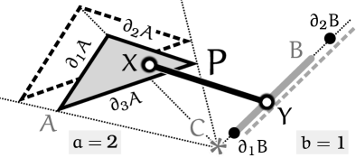
Figure 1: Crofton Reduction Technique

Proof.

The formula is a special case of the extension of the Crofton theorem by Ruben and Reed [6], although it is fairly simple to derive directly. Let $r=1+\varepsilon$ and put $C=O$ (the origin) without loss of generality. The key is to express $P_{rA,rB}$ in two different ways:

• By definition,

  $$P_{rA,rB} =\mathbb{E}\left[P(X,Y)\,|\,X\in rA,Y\in rB,\,\text{uniform}\right]=\mathbb{E}\left[P(rX^{\prime},rY^{\prime})\,|\,X^{\prime}\in A,Y^{\prime}\in B,\,\text{uniform}\right]$$

  $$=r^{p}\,\mathbb{E}\left[P(X^{\prime},Y^{\prime})\,|\,X^{\prime}\in A,Y^{\prime}\in B,\,\text{uniform}\right]=r^{p}P_{AB}=P_{AB}+\varepsilon pP_{AB}+O(\varepsilon^{2}).$$

• On the other hand,

  $$\operatorname{vol}(rA)\operatorname{vol}(rB)P_{rA,rB}=\operatorname{vol}(rA)\operatorname{vol}(rB)\mathbb{E}\left[P(X,Y)\,|\,X\in rA,Y\in rB,\,\text{uniform}\right]$$

  $$=\int_{rA}\int_{rB}P(x,y)\,\,\mathrm{d}x\mathrm{d}y=\int_{A}\int_{B}P(x,y)\,\,\mathrm{d}x\mathrm{d}y+\int_{(rA,A)}\int_{B}P(x,y)\,\,\mathrm{d}x\mathrm{d}y$$

  $$+\int_{A}\int_{(rB,B)}P(x,y)\,\,\mathrm{d}x\mathrm{d}y+\int_{(rA,A)}\int_{(rB,B)}P(x,y)\,\,\mathrm{d}x\mathrm{d}y$$

  $$=\operatorname{vol}A\operatorname{vol}BP_{AB}+\varepsilon\operatorname{vol}B\sum_{i}\operatorname{vol}(\partial_{i}A)h_{O}(\partial_{i}A)P_{\partial_{i}\,AB}$$

  $$+\varepsilon\operatorname{vol}A\sum_{j}\operatorname{vol}(\partial_{j}B)h_{O}(\partial_{j}B)P_{A\,\partial_{j}B}+O(\varepsilon^{2}).$$

Comparing the $\varepsilon$ terms of both expressions and using Remark 3, we get the statement of the lemma. If either of $\dim A$ or $\dim B$ is zero, the lemma holds too. ∎

2.2 Auxiliary integrals

Apart from rotations and reflections, any integral encountered in our paper has the following form ($h>0$)

$$I^{(p)}_{f}(h,\zeta,\gamma)=\int_{D(\zeta,\gamma)}f(x,y)\left(h^{2}+x^{2}+y^{2}\right)^{p/2}\,\,\mathrm{d}x\mathrm{d}y,$$ (6)

where $D(\zeta,\gamma)$ is the fundamental triangle domain with vertices $[0,0]$, $[\zeta,0]$, $[\zeta,\zeta\tan\gamma]$ ($\zeta>0$, $0<\gamma<\pi/2$) and $f(x,y)$ is a polynomial in $x$ and $y$ of degree at most two (quadratic in $x$ and $y$). We can write $f(x,y)=a_{00}+a_{10}x+a_{01}y+a_{20}x^{2}+a_{11}xy+a_{02}y^{2}$. Based on $x$ and $y$ terms, we have the following

$$\begin{split}I^{(p)}_{f}(h,\zeta,\gamma)&=a_{00}I^{(p)}_{00}(h,\zeta,\gamma)+a_{10}I^{(p)}_{10}(h,\zeta,\gamma)+a_{01}I^{(p)}_{01}(h,\zeta,\gamma)\\ &+a_{20}I^{(p)}_{20}(h,\zeta,\gamma)+a_{11}I^{(p)}_{11}(h,\zeta,\gamma)+a_{02}I^{(p)}_{02}(h,\zeta,\gamma),\end{split}$$ (7)

where

$$I^{(p)}_{ij}(h,\zeta,\gamma)=\int_{D(\zeta,\gamma)}x^{i}y^{j}\left(h^{2}+x^{2}+y^{2}\right)^{p/2}\,\,\mathrm{d}x\mathrm{d}y.$$ (8)

The parameters of those integrals are not optimal. We only need to consider the case $h=1$. To see this, denote

$$I^{(p)}_{ij}(q,\gamma)=I^{(p)}_{ij}(1,q,\gamma)=\int_{D(q,\gamma)}x^{i}y^{j}\left(1+x^{2}+y^{2}\right)^{p/2}\,\,\mathrm{d}x\mathrm{d}y.$$ (9)

By scaling $x\to hx$, $y\to hy$, we can write

$$I^{(p)}_{ij}(h,\zeta,\gamma)=h^{2+p+i+j}I^{(p)}_{ij}(\zeta/h,\gamma).$$ (10)

Thus, with $q=\zeta/h$,

$$\begin{split}I^{(p)}_{f}(h,\zeta,\gamma)&=h^{2+p}\big{[}a_{00}I^{(p)}_{00}(q,\gamma)+a_{10}hI^{(p)}_{10}(q,\gamma)+a_{01}hI^{(p)}_{01}(q,\gamma)\\ &+a_{20}h^{2}I^{(p)}_{20}(q,\gamma)+a_{11}h^{2}I^{(p)}_{11}(q,\gamma)+a_{02}h^{2}I^{(p)}_{02}(q,\gamma)\big{]}.\end{split}$$ (11)

Selected values of the auxiliary integrals $I^{(p)}_{ij}(q,\gamma)$ and the methods how we can derive them are found in the appendix.

3 Irreducible configurations of the reduction technique

Repeated use of the latter Lemma we refer to as the Crofton Reduction Technique. To find the moments of $L$, we put $P=L^{p}$. In the first step, we choose $A=K$ and $B=K$. Since the affine hulls of both $A$ and $B$ fill the whole space $\mathbb{R}^{d}$, any point in $\mathbb{R}^{d}$ can be selected for $C$. We then employ the reduction technique to express $P_{AB}$ in $P_{A^{\prime}B^{\prime}}$ where $A^{\prime}$ and $B^{\prime}$ have smaller dimensions then $A$ and $B$. The pairs of various $A^{\prime}$ and $B^{\prime}$ we encounter we call configurations. The process is repeated until the affine hull intersection of $A^{\prime}$ and $B^{\prime}$ is empty. In that case, we have reached an irreducible configuration. From now on in the rest of our paper if not explicitely stated, $d=3$. The following configurations are irreducible in $\mathbb{R}^{3}$:

• $A$ is a polygon and $B$ is a point

• $A$ and $B$ are two skew line segments

• $A$ and $B$ are two parallel polygons or one polygon and one line segment parallel to it

3.1 Polygon and a point

In the first case, $A$ is a polygon and $B$ a point. Denote $\operatorname{proj}_{A}(\cdot)$ a perpendicular projection onto $\mathcal{A}(A)$. Next, denote $h$ the distance between $B$ and $\mathcal{A}(A)$. With $k=x-\operatorname{proj}_{A}B$ where $x\in A$, we have that

$$L_{AB}^{(p)}=\frac{1}{\operatorname{vol}A}\int_{A}(h^{2}+k^{2})^{p/2}\,\,\mathrm{d}k$$ (12)

is expressible in terms of elementary functions. To see this, write and $\partial_{i}A,i=1,\ldots,s$ for the sides of the polygon $A$, oriented such that the path through the vertices of $A$ is counterclockwise. Then, by inclusion/exclusion, and switching to polar coordinates

$$L^{(p)}_{AB}=\frac{1}{\operatorname{vol}A}\sum_{i=1}^{s}\int_{T_{i}}(h^{2}+k^{2})^{p/2}\,\,\mathrm{d}k=\frac{1}{\operatorname{vol}A}\sum_{i=1}^{s}\int_{\alpha_{i}}^{\beta_{i}}\int_{0}^{h_{i}/\cos\varphi}(h^{2}+r^{2})^{p/2}r\,\,\mathrm{d}r\mathrm{d}\varphi$$ (13)

where $T_{i}$ is a signed triangle whose one vertex is the point $\operatorname{proj}B$ and the other two vertices are the consecutive endpoints of $\partial_{i}A$. Rescaling the vector $k$ by $h$, we can rewrite each integral in the sum in a standard way

$$\int_{T_{i}}(h^{2}+k^{2})^{p/2}\,\,\mathrm{d}k=h^{2+p}\left(I^{(p)}_{00}\left(h_{i}/h,\beta_{i}\right)-I^{(p)}_{00}\left(h_{i}/h,\alpha_{i}\right)\right)$$ (14)

where $\alpha_{i}$ and $\beta_{i}$ are their respective polar angles (in counterclockwise order) and $h_{i}$ is the perpendicular distance from $\operatorname{proj}B$ to $\partial_{i}A$. The polar angles are defined such that the closest point on the line $\mathcal{A}(\partial_{i}A)$ from $\operatorname{proj}B$ has its value equal to zero, increasing in the clockwise direction (see Figure 2). The integral is positive if the angle of consecutive vertices of the polygon increased and negative if it decreased.

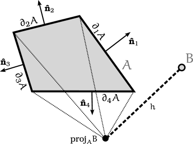
Figure 2: Point-polygon triangle decomposition

Summing all contributions, we finally get our point-polygon formula

$$L^{(p)}_{AB}=\frac{h^{2+p}}{\operatorname{vol}A}\sum_{i=1}^{s}\left(I^{(p)}_{00}\left(h_{i}/h,\beta_{i}\right)-I^{(p)}_{00}\left(h_{i}/h,\alpha_{i}\right)\right).$$ (15)

3.2 Two skewed line segments

The second case is in fact equivalent with the first. If $A$ and $B$ are two skew line segments, write $A-B=\{u-v\,|\,u\in A,v\in B\}$ (which is a parallelogram). Then, by shifting, we get for any homogeneous $P$, denoting $O$ as the origin

$$P_{AB}=P_{O,A-B}.$$ (16)

So we can always reduce this problem to the polygon and a point problem treated before.

3.3 Overlap formula

From now on, in case of no ambiguity, we often write simply $\operatorname{proj}$ instead of $\operatorname{proj}_{A}$ for the perpendicular projection operator onto $\mathcal{A}(A)$.

Proposition 4.

Let $A,B\in\mathcal{P}_{+}(\mathbb{R}^{3})$, $a=2$, $b\in\{1,2\}$, such that $\mathcal{A}(A)$ and $\mathcal{A}(B)$ are parallel with perpendicular separation vector $s$ having length $h=\|s\|$. Let $P(x,y)$ be homogeneous and let $k$ be a vector lying in the projection plane $\mathcal{A}(A)$, then

$$P_{AB}=\frac{1}{\operatorname{vol}A\operatorname{vol}B}\int_{A}\int_{B}\tilde{P}(x-y)\,\,\mathrm{d}x\mathrm{d}y=\frac{1}{\operatorname{vol}A\operatorname{vol}B}\int_{\mathbb{R}^{2}}\tilde{P}(s+k)\operatorname{vol}(A\cap(\operatorname{proj}B+k))\,\,\mathrm{d}k.$$ (17)

Especially, for $P=L^{p}$, we get $L_{AB}^{(p)}=\frac{1}{\operatorname{vol}A\operatorname{vol}B}\int_{\mathbb{R}^{2}}(h^{2}+k^{2})^{p/2}\operatorname{vol}(A\cap(\operatorname{proj}B+k))\,\,\mathrm{d}k$.

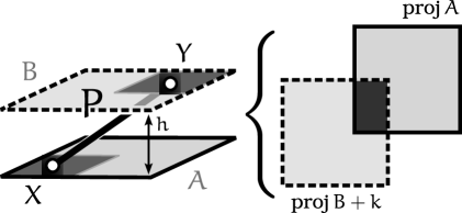
Figure 3: Overlap formula

Remark 5.

Since $\operatorname{vol}(A\cap(\operatorname{proj}B+k))$ is a piece-wise polynomial function of degree at most two on polygonal domains, the double integral is expressible in terms of elementary functions for any integer $p>-3$.

Proof.

Let $A,B\subset\mathbb{R}^{d}$ be compact domains with dimensions $a$ and $b$, respectively, and $P$ be even homogeneous function $\mathbb{R}^{d}\to\mathbb{R}$ of order $p>-3$. Let $A_{B}(z)=A\cap(B+z)$, $c=\max_{z\in\mathbb{R}^{d}}\dim A_{B}(z)$ and $C=\{z\in\mathbb{R}^{d}\,|\,\dim A_{B}(z)=c\}$. Then, by substitution $y=x+z$ and by Fubini’s theorem,

$$P_{AB}=\frac{1}{\operatorname{vol}A\operatorname{vol}B}\int_{A}\int_{B}\tilde{P}(x-y)\,\,\mathrm{d}x\mathrm{d}y=\frac{1}{\operatorname{vol}A\operatorname{vol}B}\int_{C}\tilde{P}(z)\operatorname{vol}A_{B}(z)\,\,\mathrm{d}z.$$ (18)

When $A,B$ are parallel in $d=3$, the proposition follows. ∎

Definition 7.

An overlap diagram of $A$ (face) and $B$ (parallel face or edge) consists of partitions of $\mathbb{R}^{2}$ into open subdomains $D_{i}$ where $\operatorname{vol}(A\cap(\operatorname{proj}B+k))$ can be expressed as a single polynomial function in $k$ of degree at most two. Since $A$ and $B$ are polygons (or a polygon and a polyline, respectively), these subdomains $D_{i}$ are also polygonal (polylinial, respectively). When there is no ambiguity, we denote those subdomains $D_{i}$ by numbers corresponding to the number of sides of the polygon $A\cap(\operatorname{proj}B+k)$ of intersection in case $B$ is a face, or the number of line segments of the polyline $A\cap(\operatorname{proj}B+k)$ of intersection when $B$ is an edge, respectively

Remark 6.

For brevity, we often write $\operatorname{vol}(A\cap\operatorname{proj}B+k)$ instead of $\operatorname{vol}(A\cap(\operatorname{proj}B+k))$.

4 General and special polyhedra

4.1 General polyhedra

Theorem 5.

Let $K\in\mathcal{P}(\mathbb{R}^{3})$, $E_{j},F_{k},j\in\{1,\ldots,e\},k\in\{1,\ldots,f\}$, denote the edges and faces of $K$, respectively, and let $P:\mathbb{R}^{d}\times\mathbb{R}^{d}\to\mathbb{R}$ be even and homogeneous of order $p>-3$. Then

$$P_{KK}=\frac{2}{(6+p)(5+p)}\bigg{(}\sum_{k<k^{\prime}}P_{F_{k}F_{k^{\prime}}}w_{F_{k}F_{k^{\prime}}}+\sum_{j}P_{KE_{j}}w_{KE_{j}}\bigg{)},$$ (19)

with weights $w_{AB}$ (independent on $P$ and $p$) given as follows: We fix $C$ any point in $\mathbb{R}^{3}$, $C_{k}$ any point on $\mathcal{A}(F_{k})$ and $D_{j}$ any point on $\mathcal{A}(E_{j})$. Denote $F_{k(j)},F_{k^{\prime}(j)}$ the two faces on which lies the edge $E_{j}$, then

$$w_{F_{k}F_{k^{\prime}}} =\frac{\operatorname{vol}(F_{k})\operatorname{vol}(F_{k^{\prime}})}{\operatorname{vol}^{2}\!K}(h_{C}(F_{k})h_{C_{k}}(F_{k^{\prime}})+h_{C}(F_{k^{\prime}})h_{C_{k^{\prime}}}(F_{k})),$$ (20)

$$w_{KE_{j}} =\frac{\operatorname{vol}K\operatorname{vol}(E_{j})}{\operatorname{vol}^{2}\!K}\left(h_{C}(F_{k(j)})h_{C_{k(j)}}(D_{j})+h_{C}(F_{k^{\prime}(j)})h_{C_{k^{\prime}(j)}}(D_{j})\right).$$ (21)

Proof.

Use the Crofton Reduction Technique twice. ∎

Remark 7.

Note that the weights are not unique as they depend on the position of scaling points.

Remark 8.

Note that if $P=L^{p}$ and for any polyhedron $K$, all terms $P_{AB}$ in Equation (19) are either further reducible or $A$ and $B$ are parallel. In both cases, we can express $L^{(p)}_{AB}$ in terms of auxiliary integrals. Theorem 1 follows.

4.2 Nonparallel polyhedra

For polyhedra which have some special properties, we are able to further reduce Theorem 5 above.

Definition 8.

Let $\mathcal{P}^{*}(\mathbb{R}^{3})$ denote the set of all polyhedra having the property that affine hulls of any of its three faces of meet at a single point. We call them nonparallel polyhedra. Also, we denote $\mathcal{P}_{\mathrm{convex}}^{*}(\mathbb{R}^{3})$ a subset of those which are convex.

Theorem 6.

Let $K\in\mathcal{P}^{*}(\mathbb{R}^{3})$ and $V_{i},E_{j},F_{k},i\in\{1,\ldots,v\},j\in\{1,\ldots,e\},k\in\{1,\ldots,f\}$, denote the vertices, edges and faces of $K$, respectively, and $P$ be even and homogeneous of order $p>-3$. Then

$$P_{KK}=\frac{12}{(6+p)(5+p)(4+p)(3+p)}\bigg{(}\sum_{\begin{subarray}{c}ik\\ V_{i}\notin\mathcal{A}(F_{k})\end{subarray}}P_{V_{i}F_{k}}w_{V_{i}F_{k}}+\sum_{\begin{subarray}{c}j<j^{\prime}\\ \mathcal{A}(E_{j})\cap\mathcal{A}(E_{j^{\prime}})=\emptyset\end{subarray}}P_{E_{j}E_{j^{\prime}}}w_{E_{j}E_{j^{\prime}}}\bigg{)}$$ (22)

for some weights $w_{AB}$ which are independent on $P$ and $p$.

Proof.

Since no pair of faces nor edges are parallel, we can further reduce $P_{F_{k}F_{k^{\prime}}}$ and $P_{KE_{j}}$ from Theorem 5 twice. The weights are easily computable by choosing appropriate scaling points. Note that again the weights are not unique and depend on the selection of those scaling points. For example, let $C\in\mathcal{A}(F_{k})\cap\mathcal{A}(F_{k^{\prime}})$, $k<k^{\prime}$. Then by CRT, we get

$$P_{F_{k}F_{k^{\prime}}}=\frac{2}{4+p}\left(P_{\partial F_{k}F_{k^{\prime}}}+P_{F_{k}\partial F_{k^{\prime}}}\right).$$ (23)

Note that both $P_{\partial F_{k}F_{k^{\prime}}}$ and $P_{F_{k}\partial F_{k^{\prime}}}$ are expressible as some linear combination of $P_{E_{i}F_{k}}$ with $\mathcal{A}(E_{i})\cap\mathcal{A}(F_{k})$. Finally, we can reduce even this term. Let $C^{\prime}\in\mathcal{A}(E_{i})\cap\mathcal{A}(F_{k})$, then

$$P{E_{i}F_{k}}=\frac{1}{2+p}\left(P_{\partial E_{i}F_{k}}+2P_{E_{i}\partial F_{k}}\right),$$ (24)

which in turn is expressible as a linear combination of $P_{V_{i}F_{k}}$ and $P_{E_{i}E_{i^{\prime}}}$ with $V_{i}\notin\mathcal{A}(F_{k})$ and $\mathcal{A}(E_{i})\cap\mathcal{A}(E_{i^{\prime}})=\emptyset$. The reduction of terms $P_{KE_{j}}$ is similar. ∎

4.3 Nonparallel convex polyhedra

In the case of convex nonparallel polyhedra, we can find very simple relations for weights $w_{AB}$. First, we start with a known formula (a simple generalisation of [4, Eq. 34] in $d=3$)

Lemma 7.

Let $K$ be a convex and compact set in $\mathbb{R}^{3}$ and $P$ even homogeneous of order $p>-3$, then

$$P_{KK}=\frac{1/\operatorname{vol}^{2}\!K}{(4+p)(3+p)}\oint_{B_{1}(0)}\int_{\Sigma_{\perp}(\mathbf{\hat{r}})}\tilde{P}(\mathbf{\hat{r}})\,\Lambda_{Q}^{4+p}(\mathbf{\hat{r}})\,\,\mathrm{d}Q\mathrm{d}\mathbf{\hat{r}},$$ (25)

where the integration in carried over all directions $\mathbf{\hat{r}}$ on the unit sphere $B_{1}(0)$ with surface measure $\mathrm{d}\mathbf{\hat{r}}$ having $\oint\mathrm{d}\mathbf{\hat{r}}=4\pi$ and over all points $Q$ on plane $\Sigma_{\perp}(\mathbf{\hat{r}})$ passing through the origin and being perpendicular to $\mathbf{\hat{r}}$. Finally, $\Lambda_{Q}(\mathbf{\hat{r}})$ denotes the length of the intersection of $K$ and the line passing through $Q$ in the direction of unit vector $\mathbf{\hat{r}}$.

Corollary 7.1.

By Fubini’s theorem,

$$\lim_{p\rightarrow-3^{+}}(3+p)P_{KK}=\frac{1}{\operatorname{vol}K}\oint_{B_{1}(0)}\tilde{P}(\mathbf{\hat{r}})\,\mathrm{d}\mathbf{\hat{r}}$$ (26)

Remark 9.

Similar formulae are available in higher dimensions as well.

Theorem 8.

Let $K\in\mathcal{P}_{\mathrm{convex}}^{*}(\mathbb{R}^{3})$ and $V_{i},E_{j},F_{k},P,w_{AB}$ be defined exactly as in Theorem 6. Denote $h_{ik}$ the distance between $V_{i}$ and $\mathcal{A}(F_{k})$, similarly denote $h_{jj^{\prime}}$ the distance between $O$ and $\mathcal{A}(E_{j}-E_{j^{\prime}})$ and $\theta_{jj^{\prime}}$ the angle between $E_{j}$ and $E_{j^{\prime}}$ (on the same plane under perpendicular projection). Then

$$\begin{split}P_{KK}&=\frac{12/\operatorname{vol}K}{(6+p)(5+p)(4+p)(3+p)}\bigg{(}\sum_{\begin{subarray}{c}ik\\ V_{i}\notin\mathcal{A}(F_{k})\end{subarray}}P_{V_{i}F_{k}}n_{V_{i}F_{k}}\operatorname{vol}(F_{k})h_{ik}\,\,\\ &+\!\!\!\!\sum_{\begin{subarray}{c}j<j^{\prime}\\ \mathcal{A}(E_{j})\cap\mathcal{A}(E_{j^{\prime}})=\emptyset\end{subarray}}\!P_{E_{j}E_{j^{\prime}}}n_{E_{j}E_{j^{\prime}}}\operatorname{vol}(E_{j})\operatorname{vol}(E_{j^{\prime}})h_{jj^{\prime}}\sin\theta_{jj^{\prime}}\bigg{)},\end{split}$$ (27)

with weights $n_{AB}$ satisfying the following projection relation: Choose a direction $\mathbf{\hat{n}}$ and project $K$ onto a plane perpendicular to it. Then the weights corresponding to vertex-face pairs which overlap and to pairs of edges which cross add up to one. Symbolically,

$$1=\sum_{\begin{subarray}{c}ik\\ V_{i}\notin\mathcal{A}(F_{k})\end{subarray}}n_{V_{i}F_{k}}1_{\mathbf{\hat{n}}\in V_{i}F_{k}}+\sum_{\begin{subarray}{c}j<j^{\prime}\\ \mathcal{A}(E_{j})\cap\mathcal{A}(E_{j^{\prime}})=\emptyset\end{subarray}}n_{E_{j}E_{j^{\prime}}}1_{\mathbf{\hat{n}}\in E_{j}E_{j^{\prime}}},$$ (28)

where $1_{\mathbf{\hat{n}}\in AB}$ = 1 if there are points $x\in A,y\in B$ such that $x-y$ is parallel with $\mathbf{\hat{n}}$, otherwise $1_{\mathbf{\hat{n}}\in AB}=0$. On top of that, the extreme case where one of the points $x,y$ lies on the boundary of $A$ or $B$ leaves the value $1_{\mathbf{\hat{n}}\in AB}$ undefined.

Proof.

The key observation is that the weights are independent of the choice of the function $P$ as long it is even and homogeneous. Let $\varepsilon>0$ be small and $\mathbf{\hat{n}}$ be a fixed unit vector, $\Omega_{\varepsilon}=\pi\varepsilon^{2}+O(\varepsilon^{4})$ then denotes a solid angle with apex half angle equal to $\varepsilon$. We define $R^{(p)}(\varepsilon,\mathbf{\hat{n}},x,y)=\|x-y\|^{p}$ if the angle between $\mathbf{\hat{r}}$ and $x-y$ is smaller than $\varepsilon$ and zero otherwise. Alternatively, denote $C(\varepsilon,V,\mathbf{\hat{n}})$ a double-cone region whose vertex is $V$, apex angle $2\varepsilon$ and the axis has direction $\mathbf{\hat{n}}$. Then for any domains $A$ and $B$,

$$R^{(p)}_{AB}(\varepsilon,\mathbf{\hat{n}})=\int_{A}\int_{B}R^{(p)}(\varepsilon,\mathbf{\hat{n}},x,y)\,\,\mathrm{d}y\,\,\mathrm{d}x=\int_{A}\int_{B\cap C(\varepsilon,x,\mathbf{\hat{n}})}\|x-y\|^{p}\,\,\mathrm{d}y\,\,\mathrm{d}x.$$ (29)

Note that $R$ is even and homogeneous in $x,y$ of order $p$. Hence, by Lemma 7,

$$\lim_{p\rightarrow-3^{+}}(3+p)R^{(p)}_{KK}(\varepsilon,\mathbf{\hat{n}})=\frac{1}{\operatorname{vol}K}\oint_{B_{1}(0)}\tilde{R}^{(-3)}(\varepsilon,\mathbf{\hat{n}},\mathbf{\hat{r}})\,\mathrm{d}\mathbf{\hat{r}}=\frac{2\Omega_{\varepsilon}}{\operatorname{vol}K}+O(\varepsilon^{4}).$$ (30)

On the other hand, via Theorem 6,

$$\lim_{p\rightarrow-3^{+}}(3+p)R^{(p)}_{KK}(\varepsilon,\mathbf{\hat{n}})=2\,\bigg{(}\sum_{\begin{subarray}{c}ik\\ V_{i}\notin\mathcal{A}(F_{k})\end{subarray}}R^{(-3)}_{V_{i}F_{k}}(\varepsilon,\mathbf{\hat{n}})w_{V_{i}F_{k}}+\sum_{\begin{subarray}{c}j<j^{\prime}\\ \mathcal{A}(E_{j})\cap\mathcal{A}(E_{j^{\prime}})=\emptyset\end{subarray}}R^{(-3)}_{E_{j}E_{j^{\prime}}}(\varepsilon,\mathbf{\hat{n}})w_{E_{j}E_{j^{\prime}}}\bigg{)}.$$ (31)

We are able to express $R^{(-3)}_{V_{i}F_{k}}(\varepsilon,\mathbf{\hat{n}})$ and $R^{(-3)}_{E_{j}E_{j^{\prime}}}(\varepsilon,\mathbf{\hat{n}})$ in the following way:

$$R^{(-3)}_{V_{i}F_{k}}(\varepsilon,\mathbf{\hat{n}})=\frac{\Omega_{\varepsilon}1_{\mathbf{\hat{n}}\in V_{i}F_{k}}}{\operatorname{vol}(F_{k})h_{ik}}+O(\varepsilon^{4}),\qquad R^{(-3)}_{E_{j}E_{j^{\prime}}}(\varepsilon,\mathbf{\hat{n}})=\frac{\Omega_{\varepsilon}1_{\mathbf{\hat{n}}\in E_{j}E_{j^{\prime}}}}{\operatorname{vol}(E_{j})\operatorname{vol}(E_{j^{\prime}})h_{jj^{\prime}}\sin\theta_{jj^{\prime}}}+O(\varepsilon^{4}).$$ (32)

We will prove only the first equality as the other one is get simply by shifting (edge-edge configuration is equivalent to vertex-face configuration by means of Equation (16)). Let $V_{i}\notin\mathcal{A}(F_{k})$ for some (polygonal) face $F_{k}$ and vertex $V_{i}$. We denote by $r$ the distance between $V_{i}$ and the point of intersection of $\mathcal{A}(F_{k})$ and the line passing through the vertex $V_{i}$ in the direction of $\mathbf{\hat{n}}$. Note that the perpendicular distance $h_{ik}$ between $V_{i}$ and $\mathcal{A}(F_{k})$ is independent on the direction of $\mathbf{\hat{n}}$. Since $\varepsilon$ is small, we can write

$$R^{(p)}_{V_{i}F_{k}}(\varepsilon,\mathbf{\hat{n}})=\frac{1}{\operatorname{vol}(F_{k})}\int_{F_{k}}R^{(p)}(\varepsilon,\mathbf{\hat{n}},x,V_{i})\,\,\mathrm{d}x=\frac{r^{p}\operatorname{vol}(F_{k}\cap C(\varepsilon,V_{i},\mathbf{\hat{n}}))}{\operatorname{vol}(F_{k})}+O(\varepsilon^{4})$$ (33)

Assuming $\mathbf{\hat{n}}\in V_{i}F_{k}$, the point of intersection lies in the interior of $F_{k}$. Hence, for sufficiently small $\varepsilon$, we get that $V_{i}\cap C(\varepsilon,V_{i},\mathbf{\hat{n}})$ is an ellipse with area

$$\operatorname{vol}(V_{i}\cap C(\varepsilon,V_{i},\mathbf{\hat{n}}))=1_{\mathbf{\hat{n}}\in V_{i}F_{k}}\frac{\Omega_{\varepsilon}r^{3}}{h_{ik}}+O(\varepsilon^{4})$$ (34)

Hence

$$R^{(p)}_{V_{i}F_{k}}(\varepsilon,\mathbf{\hat{n}})=\frac{1}{\operatorname{vol}(F_{k})}\int_{F_{k}}R^{(p)}(\varepsilon,\mathbf{\hat{n}},x,V_{i})\,\,\mathrm{d}x=\frac{r^{3+p}\Omega_{\varepsilon}1_{\mathbf{\hat{n}}\in V_{i}F_{k}}}{\operatorname{vol}(F_{k})h_{ik}}+O(\varepsilon^{4})$$ (35)

when $p=-3$, the dependency on $r$ vanishes. Finally, comparing this relation with (30), we get the equation for weights

$$\frac{1}{\operatorname{vol}K}=\sum_{\begin{subarray}{c}ik\\ V_{i}\notin\mathcal{A}(F_{k})\end{subarray}}\frac{w_{V_{i}F_{k}}1_{\mathbf{\hat{n}}\in V_{i}F_{k}}}{\operatorname{vol}(F_{k})h_{ik}}+\sum_{\begin{subarray}{c}j<j^{\prime}\\ \mathcal{A}(E_{j})\cap\mathcal{A}(E_{j^{\prime}})=\emptyset\end{subarray}}\frac{w_{E_{j}E_{j^{\prime}}}1_{\mathbf{\hat{n}}\in E_{j}E_{j^{\prime}}}}{\operatorname{vol}(E_{j})\operatorname{vol}(E_{j^{\prime}})h_{jj^{\prime}}\sin\theta_{jj^{\prime}}}$$ (36)

valid for any $\mathbf{\hat{n}}$ for which all the values $1_{\mathbf{\hat{n}}\in AB}$ are well defined. Lastly, defining auxiliary weight $n_{AB}$ via

$$w_{V_{i}F_{k}}=\frac{\operatorname{vol}(F_{k})h_{ik}n_{V_{i}F_{k}}}{\operatorname{vol}K},\qquad w_{E_{j}E_{j^{\prime}}}=\frac{\operatorname{vol}(E_{j})\operatorname{vol}(E_{j^{\prime}})h_{jj^{\prime}}n_{E_{j}E_{j^{\prime}}}\sin\theta_{jj^{\prime}}}{\operatorname{vol}K},$$ (37)

we get

$$1=\sum_{\begin{subarray}{c}ik\\ V_{i}\notin\mathcal{A}(F_{k})\end{subarray}}n_{V_{i}F_{k}}1_{\mathbf{\hat{n}}\in V_{i}F_{k}}+\sum_{\begin{subarray}{c}j<j^{\prime}\\ \mathcal{A}(E_{j})\cap\mathcal{A}(E_{j^{\prime}})=\emptyset\end{subarray}}n_{E_{j}E_{j^{\prime}}}1_{\mathbf{\hat{n}}\in E_{j}E_{j^{\prime}}}.$$ (38)

This constrain alone enables us to determine admissible weights for any convex nonparallel polyhedron via set of linear equations got by varying the direction of $\mathbf{\hat{n}}$. ∎

4.4 Tetrahedron

As an example, we express the random distance moments in the case of a tetrahedron. There are two possible ways how a planar projection of a tetrahedron could look like (almost surely) with respect to the number of intersecting pairs of edges and vertices/faces in the projection (see Figure 4).

Figure 4: Tetrahedron projection orientations

In the first case, one vertex covers one face. There are no other vertex/face nor edge/edge coverings. Similarly, in the second case, one edge is covered by another edge. There are again no other coverings. Thus, in order to satisfy Equation (28), we can simply choose $n_{V_{i}F_{k}}=n_{E_{j}E_{j^{\prime}}}=1$ for each vertex $V_{i}$, face $F_{k}$ and edges $E_{j},E_{j^{\prime}}$. Hence, by Theorem 8,

$$\begin{split}P_{KK}&=\frac{12/\operatorname{vol}K}{(6+p)(5+p)(4+p)(3+p)}\bigg{(}\sum_{\begin{subarray}{c}ik\\ V_{i}\notin\mathcal{A}(F_{k})\end{subarray}}P_{V_{i}F_{k}}\operatorname{vol}(F_{k})h_{ik}\,\,\\ &+\!\!\!\!\sum_{\begin{subarray}{c}j<j^{\prime}\\ \mathcal{A}(E_{j})\cap\mathcal{A}(E_{j^{\prime}})=\emptyset\end{subarray}}\!P_{E_{j}E_{j^{\prime}}}\operatorname{vol}(E_{j})\operatorname{vol}(E_{j^{\prime}})h_{jj^{\prime}}\sin\theta_{jj^{\prime}}\bigg{)}.\end{split}$$ (39)

5 Mean distance in regular polyhedra

To apply our general method, we shall derive the mean distance in all five regular polyhedra (also known as Platonic solids). Among those solids, only the tetrahedron is nonparallel convex, so Theorem 8 applies here. Hence, we used this theorem to find the mean distance in a general (possibly irregular) tetrahedron. In the rest of our paper, we calculate the mean distance in all other Platonic solids (including the regular tetrahedron again). Since they are an example of parallel polyhedra, we cannot use Theorem 8 due to presence of irreducible configurations of type face-face and edge-face. However, we can still calculate the mean distance. The calculation relies the Overlap formula as well as the symmetries of those regular polyhedra which drastically reduce the number of configurations needed to be considered. Throughout this section, we denote $\nu$ the area of (any) face of $K$ and $l$ the length (any) of its edge. These values makes sense because $K$ is a regular polyhedron. Furthermore, $\phi=\frac{1+\sqrt{5}}{2}$ is the Golden ratio.

5.1 Regular tetrahedron

Let us have $P$ even homogeneous of order $p$ dependent on two random points picked from $K$ a regular tetrahedron given by vertices $V_{1}[1,0,0]$, $V_{2}[0,1,0]$, $V_{3}[0,0,1]$, $V_{4}[1,1,1]$, edges connecting them $E_{12}$, $E_{13}$, $E_{14}$, $E_{23}$, $E_{24}$, $E_{34}$ ($E_{ij}=\overline{V_{i}V_{j}},$ where $i\neq j$) and with opposite faces $F_{1}$, $F_{2}$, $F_{3}$, $F_{4}$. Note that $\operatorname{vol}K=1/3$, so if we want to express the mean of $P$ in a tetrahedron of unit volume, we must multiply all our results by $3^{p/3}$. We put $P=L^{p}$. For the definition of various mean values $P_{ab}=L_{ab}^{(p)}$, see Figure 5. We also included the position of the scaling point $C$ in cases reduction is possible. The arrows indicate which configurations reduce to which.

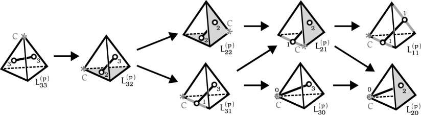
Figure 5: All different $L_{ab}^{(p)}$ configurations encountered for $K$ being a regular tetrahedron

Based on CRT, let us write our reduction system of equations:

$$pP_{33} =6(P_{32}-P_{33})$$

$$pP_{32} =3(P_{22}-P_{32})+2(P_{31}-P_{32})$$

$$pP_{22} =4(P_{21}-P_{22})$$

$$pP_{31} =3(P_{21}-P_{31})+1(P_{30}-P_{31})$$

$$pP_{21} =2(P_{11}-P_{21})+1(P_{20}-P_{21})$$

$$pP_{30} =3(P_{20}-P_{30}),$$

where $P_{33}=P_{KK}$ and by symmetry, we can put $P_{32}=P_{KF_{1}},P_{31}=P_{KE_{12}},P_{30}=P_{KV_{1}},P_{22}=P_{F_{1}F_{2}},P_{21}=P_{F_{4}V_{14}},P_{20}=P_{F_{4}V_{4}},P_{11}=P_{E_{12}E_{34}}$. This linear system has a solution

$$P_{33}=\frac{72(3P_{11}+2P_{20})}{(6+p)(5+p)(4+p)(3+p)}.$$ (40)

To demonstrate our technique for irreducible configurations, we derive the value of $L_{33}$. That means, we choose $P=L^{p}$ with $p=1$.

5.1.1 L₂₀

By (15), by symmetry and using $\operatorname{vol}(F_{4})=\sqrt{3}/2,h_{1}=1/\sqrt{6},h=2/\sqrt{3}$,

$$P_{20}=L^{(p)}_{F_{4}V_{4}}=\frac{6h^{2+p}}{\operatorname{vol}(F_{4})}I^{(p)}_{00}\left(\frac{\sqrt{2}}{4},\frac{\pi}{3}\right).$$ (41)

Using the recursion relations,

$$I^{(1)}_{00}\left(\frac{\sqrt{2}}{4},\frac{\pi}{3}\right)=\frac{1}{16\sqrt{2}}-\frac{\pi}{9}+\frac{1}{3}\arcsin\sqrt{\frac{2}{3}}+\frac{25}{96\sqrt{2}}\operatorname{arcsinh}\frac{1}{\sqrt{3}},$$ (42)

so, further using $\arcsin\sqrt{2/3}=\arctan\sqrt{2}$ and $\operatorname{arcsinh}(1/\sqrt{3})=\tfrac{1}{2}\ln 3$,

$$L_{20}=\frac{\sqrt{2}}{3}-\frac{32\pi}{27}+\frac{32}{9}\arctan\sqrt{2}+\frac{25\ln 3}{18\sqrt{2}}.$$ (43)

5.1.2 L₁₁

By shifting (16), we get $L_{11}=L_{AB}$, where $B$ is the origin and $A$ is a parallelogram with vertices $[1,0,-1],[0,1,-1]$, $[-1,0,-1]$, $[0,-1,-1]$. Therefore, by the point-polygon formula (15) with $h=1$ and $\operatorname{vol}A=2$,

$$L_{11}=\frac{8h^{3}}{\operatorname{vol}A}I^{(1)}_{00}\left(\frac{\sqrt{2}}{2},\frac{\pi}{4}\right),$$ (44)

where by recurrences,

$$I^{(1)}_{00}\left(\frac{\sqrt{2}}{2},\frac{\pi}{4}\right)=\frac{1}{6\sqrt{2}}-\frac{\pi}{12}+\frac{1}{3}\arcsin\frac{1}{\sqrt{3}}+\frac{7}{12\sqrt{2}}\operatorname{arcsinh}\frac{1}{\sqrt{3}}.$$ (45)

Hence, writing $\arcsin\left(1/\sqrt{3}\right)=\frac{\pi}{2}-\arctan\sqrt{2}$ and $\operatorname{arcsinh}(1/\sqrt{3})=\tfrac{1}{2}\ln 3$,

$$L_{11}=\frac{\sqrt{2}}{3}+\frac{\pi}{3}-\frac{4}{3}\arctan\sqrt{2}+\frac{7\ln 3}{6\sqrt{2}}.$$ (46)

5.1.3 L₃₃

Substituting $L_{20}$ and $L_{11}$ into (40) with $P=L^{p}$ and $p=1$, we get, finally

$$L_{33}=\frac{3}{35}(3L_{11}+2L_{20})=\frac{\sqrt{2}}{7}-\frac{37\pi}{315}+\frac{4}{15}\arctan\sqrt{2}+\frac{113\ln 3}{210\sqrt{2}}.$$

Or, re-scaling to the unit volume tetrahedron,

$$L_{33}\big{|}_{\operatorname{vol}K=1}=\sqrt[3]{3}\left(\frac{\sqrt{2}}{7}-\frac{37\pi}{315}+\frac{4}{15}\arctan\sqrt{2}+\frac{113\ln 3}{210\sqrt{2}}\right)\approx 0.72946242,$$ (47)

which is an exact expression of an approximation given by Weisstein [7]. Similarly, we would proceed in the case of the second moment:

$$L_{33}^{(2)}\big{|}_{\operatorname{vol}K=1}=\frac{9}{10\sqrt[3]{3}}.$$ (48)

Alternatively, we can express the result as the normalised mean distance $\Gamma_{KK}$. Since $V_{1}(K)=3\sqrt{2}\arccos\left(-\frac{1}{3}\right)/\pi$ (see Table 3 with $a=\sqrt{2}$), we have

$$\Gamma_{KK}=\frac{L_{33}}{V_{1}(K)}=\frac{\pi}{3\sqrt{2}\arccos\left(-\frac{1}{3}\right)}\left(\frac{\sqrt{2}}{7}-\frac{37\pi}{315}+\frac{4}{15}\arctan\sqrt{2}+\frac{113\ln 3}{210\sqrt{2}}\right)\approx 0.19601928.$$ (49)

Of course, using the reduction technique, we could get other moments (replacing $I_{ij}^{(1)}$ by $I_{ij}^{(p)}$ integrals), and even for a general edge-length tetrahedron.

5.2 Cube

We present a re-derivation of the Robbins constant for $K$ being a cube via our method. Here, we demonstrate the Crofton Reduction Technique including the overlap formula. A standard way how to choose its vertices is $[0,0,0]$, $[1,0,0]$, $[0,1,0]$, $[0,0,1]$, $[0,1,1]$, $[1,0,1]$, $[1,1,0]$, $[1,1,1]$. Under this choice, the edge length $l=1$, face area $\nu=1$ and the volume $\operatorname{vol}K=1$. We put $P=L^{p}$. For the definition of various mean values $P_{ab}=L_{ab}^{(p)}$, see Figure 6. Note that in $L_{21r}$ configuration, we let $B$ to be four edges (boundary of an opposite face) rather than just one edge.

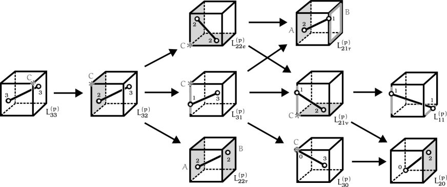
Figure 6: All different $L_{ab}^{(p)}$ configurations encountered for $K$ being a cube

Performing the reduction, we get the set of equations, where

$$pP_{33} =6(P_{32}-P_{33}),$$

$$pP_{32} =3(P_{22}-P_{32})+2(P_{31}-P_{32}),$$

$$pP_{22e} =4(P_{21}^{\prime}-P_{22e}),$$

$$pP_{31} =3(P_{21}-P_{31})+1(P_{30}-P_{31}),$$

$$pP_{21v} =2(P_{11}-P_{21v})+1(P_{20}-P_{21v}),$$

$$pP_{30} =3(P_{20}-P_{30})$$

with

$$P_{22} =\tfrac{2}{3}P_{22e}+\tfrac{1}{3}P_{22r},$$

$$P_{21} =\tfrac{1}{3}P_{21v}+\tfrac{2}{3}P_{21r},$$

$$P_{21}^{\prime} =\tfrac{1}{2}P_{21v}+\tfrac{1}{2}P_{21r}.$$

Solving the system, we get

$$P_{33}=\frac{72(P_{11}+P_{20})}{(3+p)(4+p)(5+p)(6+p)}+\frac{48P_{21r}}{(4+p)(5+p)(6+p)}+\frac{6P_{22r}}{(5+p)(6+p)}.$$ (50)

When $p=1$, we get for the mean distance

$$L_{33}=\frac{1}{35}(3L_{11}+3L_{20}+8L_{21r}+5L_{22r}).$$ (51)

5.2.1 L₂₀

Without loss of generality, we can write $L_{20}=L_{AB}$, where $A$ is the cube’s upper face defined as a square with vertices $[0,0,1]$, $[1,0,1]$, $[1,1,1]$, $[0,1,1]$ and $B$ is the origin $[0,0,0]$. Domains $A$ and $B$ are separated by distance $h=1$. The face $A$ is having area $\operatorname{vol}A=1$. By (15) and by symmetry,

$$L_{20}=\frac{2}{\operatorname{vol}A}I^{(1)}_{00}\left(1,\frac{\pi}{4}\right).$$ (52)

Using recurrence relations (see Table 5 in Appendix),

$$L_{20}=\frac{1}{\sqrt{3}}-\frac{\pi}{18}+\frac{4}{3}\operatorname{arccoth}\sqrt{3}.$$ (53)

5.2.2 L₁₁

The value $L_{11}$ can be defined as a mean distance between egde $E_{1}=\overline{[0,0,0][0,1,0]}$ and edge $E_{2}=\overline{[0,1,1][1,1,1]}$. Shifting $E_{1}$ by vector $-E_{2}$ (See shifting relation (16)), we can rewrite this as $L_{11}=L_{AB}$, where again $A$ is the upper face of the cube and $B$ is the origin. Hence $L_{11}=L_{20}$.

5.2.3 L_21r

Since the reduction technique cannot be applied on $AB$ being parallel, we use the overlap formula with $A$ being one face of the cube. In case of $L_{21r}$, the other domain $B$ is an opposite edge. By symmetry, we can add to this edge also three other edges opposite to $A$ (see Figure 6). Hence, $B$ is a boundary of the face opposite to $A$ with length $\operatorname{vol}B=4$. Let $k=(x,y)$ then $\operatorname{proj}A=\operatorname{proj}B$ is a square with vertices $[\frac{1}{2},\frac{1}{2}]$, $[-\frac{1}{2},\frac{1}{2}]$, $[-\frac{1}{2},-\frac{1}{2}]$, $[\frac{1}{2},-\frac{1}{2}]$. In order to $\operatorname{proj}A$ and $\operatorname{proj}B+k$ have nonzero intersection, $k$ must be confined in the region $-1<x<1\land-1<y<1$. By symmetry, we can chose $k$ to lie in the fundamental triangle domain $D(1,\pi/4)$ (we then multiply the values by $8$).

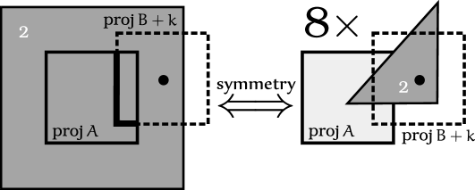
Figure 7: Overlap of the opposite face and edges of a cube

Setting up the integral,

$$L_{21r}=\frac{8}{\operatorname{vol}A\operatorname{vol}B}\int_{D}\sqrt{h^{2}+k^{2}}\operatorname{vol}(A\cap\operatorname{proj}B+k)\,\,\mathrm{d}k,$$ (54)

where $h=1,\operatorname{vol}A=1,\operatorname{vol}B=4$ and $D=D(1,\pi/4)$ is a domain in Figure 7 on the right (labeled with the number $2$). In this domain, we can write for the length of the polyline of intersection

$$\operatorname{vol}(A\cap\operatorname{proj}B+k)=2-x-y,$$ (55)

which gives us in terms of our auxiliary integrals

$$L_{21r}=\frac{8}{\operatorname{vol}A\operatorname{vol}B}\Bigg{[}2I^{(1)}_{00}\left(1,\frac{\pi}{3}\right)-I^{(1)}_{10}\left(1,\frac{\pi}{4}\right)-I^{(1)}_{01}\left(1,\frac{\pi}{4}\right)\Bigg{]}$$ (56)

Via recursions (see Table 5 in Appendix), we get

$$L_{21r}=\frac{7}{6\sqrt{2}}-\frac{1}{\sqrt{3}}-\frac{\pi}{9}+\frac{1}{4}\operatorname{arccoth}\sqrt{2}+\frac{5}{3}\operatorname{arccoth}\sqrt{3}.$$ (57)

5.2.4 L_22r

Again, we use the overlap formula for $AB$ being opposite faces. By symmetry, we again integrate $\operatorname{vol}(A\cap\operatorname{proj}B+k)$ over one eighth of all positions of $k$ (see Figure 8).

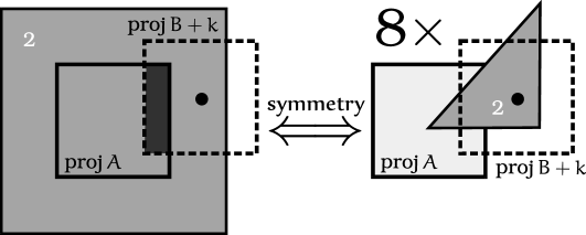
Figure 8: Overlap of the opposite faces of a cube

Setting up the integral,

$$L_{22r}=\frac{8}{\operatorname{vol}A\operatorname{vol}B}\int_{D}\sqrt{h^{2}+k^{2}}\operatorname{vol}(A\cap\operatorname{proj}B+k)\,\,\mathrm{d}k,$$ (58)

where $h=1,\operatorname{vol}A=\operatorname{vol}B=1$ and $D=D()$ is a fundamental triangle domain (labeled $2$ in Figure 11 on the right). In this domain, we have for the polygon of intersection

$$\operatorname{vol}(A\cap\operatorname{proj}B+k)=(1-x)(1-y),$$ (59)

and therefore

$$L_{22r}=\frac{8}{\operatorname{vol}A\operatorname{vol}B}\Bigg{[}I^{(1)}_{00}\left(1,\frac{\pi}{4}\right)-I^{(1)}_{10}\left(1,\frac{\pi}{4}\right)-I^{(1)}_{01}\left(1,\frac{\pi}{4}\right)+I^{(1)}_{11}\left(1,\frac{\pi}{4}\right)\Bigg{]}.$$ (60)

Going through all recursions, we get, after simplifications

$$L_{22r}=\frac{4}{15}+\frac{\sqrt{2}}{5}-\frac{4}{5\sqrt{3}}-\frac{2\pi}{9}+\operatorname{arccoth}\left(\sqrt{2}\right)+\frac{4}{3}\operatorname{arccoth}\sqrt{3}.$$ (61)

5.2.5 L₃₃

Putting everything together by using (64), we finally arrive at the Robin’s constant

$$L_{33}=\frac{4}{105}+\frac{17\sqrt{2}}{105}-\frac{2\sqrt{3}}{35}-\frac{\pi}{15}+\frac{1}{5}\operatorname{arccoth}\sqrt{2}+\frac{4}{5}\operatorname{arccoth}\sqrt{3}\approx 0.66170718.$$ (62)

5.3 Regular octahedron

A standard way how to select vertices of an regular octahedron the vertices is $\left[\pm 1,0,0\right]$, $\left[\pm 1,0,0\right]$, $\left[\pm 1,0,0\right]$. Under this choice, the edge length is $l=\sqrt{2}$, the area of each face is $\nu=\sqrt{3}/2$ and the volume of $K$ is $\operatorname{vol}K=4/3$. Again, we put $P=L^{p}$. For the definition of various mean values $P_{ab}=L_{ab}^{(p)}$, see Figure 9. We also included the position of the scaling point $C$ in cases when the reduction is possible.

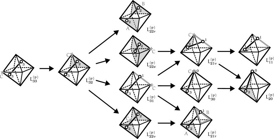
Figure 9: All different $L_{ab}^{(p)}$ configurations encountered for $K$ being a regular octahedron

Performing the reduction, we get the set of equations, where

$$pP_{33} =6(P_{32}-P_{33}),$$

$$pP_{32} =3(P_{22}-P_{32})+2(P_{31}-P_{32}),$$

$$pP_{22e} =4(P_{21v}-P_{22e}),$$

$$pP_{22v} =4(P_{21r}-P_{22v}),$$

$$pP_{31} =3(P_{21}-P_{31})+1(P_{30}-P_{31}),$$

$$pP_{21v} =2(P_{11}-P_{21v})+1(P_{20}-P_{21v}),$$

$$pP_{30} =3(P_{20}-P_{30})$$

with

$$P_{22} =\tfrac{1}{4}P_{22e}+\tfrac{1}{4}P_{22r}+\tfrac{1}{2}P_{22v},$$

$$P_{21} =\tfrac{1}{2}P_{21v}+\tfrac{1}{2}P_{21r}.$$

Solving the system, we get

$$P_{33}=\frac{72(P_{20}+P_{11})}{(3+p)(4+p)(5+p)(6+p)}+\frac{54P_{21r}}{(4+p)(5+p)(6+p)}+\frac{9P_{22r}}{2(5+p)(6+p)}.$$ (63)

When $p=1$, we get for the mean length

$$L_{33}=\frac{3}{140}(4L_{20}+4L_{11}+12L_{21r}+5L_{22r}).$$ (64)

5.3.1 L₂₀

More precisely, we can write $L_{20}=L_{AB}$, where face $A$ has vertices $[-1,0,0]$, $[0,-1,0]$, $[0,0,-1]$ and $B=[0,0,1]$ (see Figure 9). Vertex $B$ is separated from $\mathcal{A}(A)$ by distance $h=2/\sqrt{3}$. By (15) and by symmetry,

$$L_{20}=\frac{2h^{3}}{\operatorname{vol}A}\left(I^{(1)}_{00}\left(\frac{\sqrt{2}}{2},\frac{\pi}{3}\right)-I^{(1)}_{00}\left(\frac{\sqrt{2}}{4},\frac{\pi}{3}\right)\right),$$ (65)

where $\operatorname{vol}A=\nu=\sqrt{3}/2$ is the area of $A$. Using recurrence relations on $I^{{(1)}}_{00}(\cdot,\cdot)$,

$$I^{(1)}_{00}\left(\frac{\sqrt{2}}{2},\frac{\pi}{3}\right)=\frac{1}{4}-\frac{\pi}{36}+\frac{7\operatorname{arcsinh}1}{12\sqrt{2}}=\frac{1}{4}-\frac{\pi}{36}+\frac{7\operatorname{arccoth}\sqrt{2}}{12\sqrt{2}}.$$ (66)

The other $I^{(1)}_{00}$ integral is already given by (42) (we just write $\arcsin\sqrt{2/3}=\pi/2-\operatorname{arccot}\sqrt{2}$), hence

$$L_{20}=\frac{8}{9}-\frac{\sqrt{2}}{9}-\frac{8\pi}{27}-\frac{25\ln 3}{54\sqrt{2}}+\frac{32}{27}\operatorname{arccot}\sqrt{2}+\frac{28}{27}\sqrt{2}\operatorname{arccoth}\sqrt{2}$$ (67)

5.3.2 L₁₁

By shifting (16), we get $L_{11}=L_{AB}$, where $B$ is the origin and $A$ is a parallelogram with vertices $[1,0,1]$, $[0,1,1]$, $[0,2,0]$, $[1,1,0]$. Therefore, by the point-polygon formula (15) with $h=2/\sqrt{3}$ and $\operatorname{vol}A=\sqrt{3}$,

$$L_{11}=\frac{h^{3}}{\operatorname{vol}A}\left(4I^{(1)}_{00}\left(\frac{\sqrt{2}}{4},\frac{\pi}{3}\right)+2I^{(1)}_{00}\left(\frac{\sqrt{2}}{2},\frac{\pi}{3}\right)\right),$$ (68)

Hence, since the $I$’s are already given by (42) and (66), we get, simplifying,

$$L_{11}=\frac{4}{9}+\frac{\sqrt{2}}{9}+\frac{4\pi}{27}+\frac{25\ln 3}{54\sqrt{2}}-\frac{32}{27}\operatorname{arccot}\sqrt{2}+\frac{14}{27}\sqrt{2}\operatorname{arccoth}\sqrt{2}$$ (69)

5.3.3 L_21r

Since the reduction technique cannot be applied on $AB$ being parallel, we use the overlap formula with $A$ being one face of the octahedron. By symmetry, we can choose $B$ as all three opposite edges to $A$ instead of just one, the mean value stays the same (see Figure 9). This choice makes the overlap formula simpler. To compute $\operatorname{vol}(A\cap\operatorname{proj}B+k)$, we slide the projection $B$ across $A$. To get $L_{21r}$, we then integrate over the length of their intersection with respect to all vectors $k$. By symmetry, we can integrate over just one sixth of all sliding domains (see Figure 10 for our overlap diagram, in which white numbers represent the number of line segments in the $AB$ projection intersection with respect to position of the shift vector $k$ – black dot).

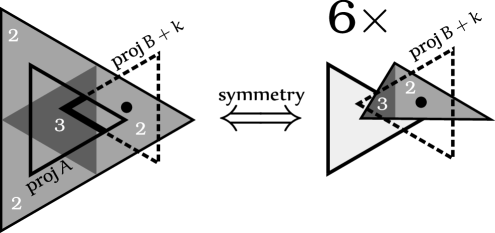
Figure 10: Overlap of the opposite face and edges of an octahedron

Hence, setting up the integral,

$$L_{21r}=\frac{6}{\operatorname{vol}A\operatorname{vol}B}\int_{D}\sqrt{h^{2}+k^{2}}\operatorname{vol}(A\cap\operatorname{proj}B+k)\,\,\mathrm{d}k,$$ (70)

where $h=2/\sqrt{3},\operatorname{vol}A=\sqrt{3}/2,\operatorname{vol}B=3\sqrt{2}$ and $D$ is a domain in Figure 10 on the right consisted of two subdomains $D_{j}$ where $j\in\{2,3\}$ denotes the number of line segments of the intersection $A\cap(\operatorname{proj}B+k)$, which is a polyline. We have $D=D_{2}\sqcup D_{3}$. Let $k=(x,y)$ with the origin coinciding with the centroid of $\operatorname{proj}A$ triangle with vertices $[0,\frac{\sqrt{6}}{3}]$, $[-\frac{\sqrt{6}}{2},\frac{\sqrt{2}}{2}]$, $[-\frac{\sqrt{6}}{2},-\frac{\sqrt{2}}{2}]$ (see Figure 10). Let us denote $v_{j}=\operatorname{vol}(A\cap\operatorname{proj}B+k)$ for all $k\in D_{j}$, then we have for the subdomains:

• $D_{3}$ is a triangle with vertices $[0,0]$, $[\frac{\sqrt{6}}{6},0]$, $[\frac{\sqrt{6}}{6},\frac{\sqrt{2}}{2}]$ in which $v_{3}=\sqrt{2}$

• $D_{2}$ is a triangle with vertices $[\frac{\sqrt{6}}{6},0]$, $[\frac{2\sqrt{6}}{3},0]$, $[\frac{\sqrt{6}}{6},\frac{\sqrt{2}}{2}]$ in which $v_{2}=\frac{4\sqrt{2}}{3}-\frac{2x}{\sqrt{3}}$

Note that in general, $\operatorname{vol}(A\cap\operatorname{proj}B+k)$ is linear in $(x,y)$ in the subdomains. By inclusion/exclusion, we can write our integral as

$$\begin{split}&L_{21r}=\frac{6}{\operatorname{vol}A\operatorname{vol}B}\left[\iint_{D_{3}\cup D_{2}}v_{2}\sqrt{h^{2}+x^{2}+y^{2}}\,\,\mathrm{d}x\mathrm{d}y+\iint_{D_{3}}\left(v_{3}-v_{2}\right)\sqrt{h^{2}+x^{2}+y^{2}}\,\,\mathrm{d}x\mathrm{d}y\right]\\ &\!=\!\frac{6}{\operatorname{vol}A\operatorname{vol}B}\!\left[\iint_{\!D_{3}\cup D_{2}}\!\!\left(\!\frac{4\sqrt{2}}{3}\!-\!\frac{2x}{\sqrt{3}}\!\right)\!\!\sqrt{h^{2}\!+\!x^{2}\!+\!y^{2}}\mathrm{d}x\mathrm{d}y\!+\!\!\!\iint_{\!D_{3}}\!\!\left(\!\frac{2x}{\sqrt{3}}\!-\!\frac{\sqrt{2}}{3}\!\right)\!\!\sqrt{h^{2}\!+\!x^{2}\!+\!y^{2}}\mathrm{d}x\mathrm{d}y\right].\end{split}$$ (71)

Note that the second integral over domain $3$ is already in the form of an integral over standard fundamental triangle domain since $D_{3}=D(\frac{\sqrt{6}}{6},\frac{\pi}{3})$. The first integral over domain $3\cup 2$ can be written in such manner after rotation and reflection. To obtain the correct transformation, we let $\varphi^{\prime}$ to start (be zero) for the half-line connecting the origin with point $[\frac{1}{\sqrt{6}},\frac{\sqrt{2}}{2}]$, increasing in the clockwise direction. That is $\varphi=\pi/3-\varphi^{\prime}$ and thus $x=r\cos(\frac{\pi}{3}-\varphi^{\prime})$ and $y=r\sin(\frac{\pi}{3}-\varphi^{\prime})$. Expanding out the trigonometric functions and writing $x^{\prime}=r\cos\varphi^{\prime}$ and $y^{\prime}=r\cos\varphi^{\prime}$, we get

$$\begin{split}x&=r\cos\frac{\pi}{3}\cos\varphi^{\prime}+r\sin\frac{\pi}{3}\sin\varphi^{\prime}=x^{\prime}\cos\frac{\pi}{3}+y^{\prime}\sin\frac{\pi}{3}=\frac{1}{2}x^{\prime}+\frac{\sqrt{3}}{2}y^{\prime},\\ y&=r\sin\frac{\pi}{3}\cos\varphi^{\prime}-r\cos\frac{\pi}{3}\sin\varphi^{\prime}=x^{\prime}\sin\frac{\pi}{3}-y^{\prime}\cos\frac{\pi}{3}=\frac{\sqrt{3}}{2}x^{\prime}-\frac{1}{2}y^{\prime}\end{split}$$ (72)

and so

$$v_{2}=\frac{4\sqrt{2}}{3}-\frac{2x}{\sqrt{3}}=\frac{4\sqrt{2}}{3}-\frac{x^{\prime}}{\sqrt{3}}-y^{\prime}.$$ (73)

Our integration domain $D_{3}\sqcup D_{2}$ in $(x^{\prime},y^{\prime})$ is simply $D(\frac{\sqrt{6}}{3},\frac{\pi}{3})$. Note that $x^{2}+y^{2}$ is invariant with respect to this transformation so $x^{2}+y^{2}=x^{\prime 2}+y^{\prime 2}$. By scaling with $h$, we can write $L_{21r}$ in terms of the auxiliary integrals as

$$\begin{split}L_{21r}=\frac{6h^{3}}{\operatorname{vol}A\operatorname{vol}B}\Bigg{[}&\frac{4\sqrt{2}}{3}I^{(1)}_{00}\left(\frac{\sqrt{6}}{3h},\frac{\pi}{3}\right)-\frac{h}{\sqrt{3}}I^{(1)}_{10}\left(\frac{\sqrt{6}}{3h},\frac{\pi}{3}\right)-hI^{(1)}_{01}\left(\frac{\sqrt{6}}{3h},\frac{\pi}{3}\right)\\ &+\frac{2h}{\sqrt{3}}I^{(1)}_{10}\left(\frac{\sqrt{6}}{6h},\frac{\pi}{3}\right)-\frac{\sqrt{2}}{3}I^{(1)}_{00}\left(\frac{\sqrt{6}}{6h},\frac{\pi}{3}\right)\Bigg{]}\end{split}$$ (74)

with $\frac{\sqrt{6}}{3h}=\frac{\sqrt{2}}{2}$ and $\frac{\sqrt{6}}{6h}=\frac{\sqrt{2}}{4}$. Via recursions (see Table 5 in Appendix), we get

$$L_{21r}=-\frac{10}{27}+\frac{47}{54\sqrt{2}}-\frac{16\pi}{81}+\frac{143\ln 3}{648\sqrt{2}}+\frac{32}{81}\operatorname{arccot}\sqrt{2}+\frac{85}{81}\sqrt{2}\operatorname{arccoth}\sqrt{2}$$ (75)

5.3.4 L_22r

Again, we use the overlap formula for $A$ and $B$ being opposite faces of $K$. By symmetry, we again integrate $\operatorname{vol}(A\cap\operatorname{proj}B+k)$ over one sixth of all positions of vector $k$ (see Figure 11, in which white numbers represent the number of sides of a polygon of intersection of $AB$ projections with respect to position of the shift vector $k$ – black dot).

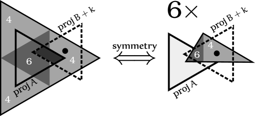
Figure 11: Overlap of the opposite faces of an octahedron

Setting up the integral,

$$L_{22r}=\frac{6}{\operatorname{vol}A\operatorname{vol}B}\int_{D}\sqrt{h^{2}+k^{2}}\operatorname{vol}(A\cap\operatorname{proj}B+k)\,\,\mathrm{d}k,$$ (76)

where $h=2/\sqrt{3},\operatorname{vol}A=\operatorname{vol}B=\nu=\sqrt{3}/2$ and $D$ is a domain in Figure 11 on the right consisted of two subdomains labeled $6$ and $4$ according to the number of sides of the intersection (which is a polygon). That is, $D=D_{6}\sqcup D_{4}$. Let $k=(x,y)$ and denote $v_{j}=\operatorname{vol}(A\cap\operatorname{proj}B+k)$ for those $k$ which lie in $\in D_{j}$, then the subdomain

• $D_{6}$ is again a triangle with vertices $[0,0]$, $[\frac{\sqrt{6}}{6},0]$, $[\frac{\sqrt{6}}{6},\frac{\sqrt{2}}{2}]$ in which $v_{6}=\frac{1}{\sqrt{3}}-\frac{\sqrt{3}}{2}x^{2}-\frac{\sqrt{3}}{2}y^{2}$

• $D_{4}$ is a triangle with vertices $[\frac{\sqrt{6}}{6},0]$, $[\frac{2\sqrt{6}}{3},0]$, $[\frac{\sqrt{6}}{6},\frac{\sqrt{2}}{2}]$ in which $v_{4}=\frac{4}{3\sqrt{3}}-\frac{2\sqrt{2}x}{3}+\frac{x^{2}}{2\sqrt{3}}-\frac{\sqrt{3}y^{2}}{2}$

Domains $6,4$ coincide with $3,2$ in $L_{21r}$ case, that is $D_{6}=D_{3}$ and $D_{4}=D_{2}$. Note that in general, $\operatorname{vol}(A\cap\operatorname{proj}B+k)$ is quadratic in $(x,y)$ in the subdomains. By inclusion/exclusion, we can write the integral as

$$\begin{split}L_{22r}=\frac{6}{\operatorname{vol}A\operatorname{vol}B}\Big{[}&\iint_{D_{6}\cup D_{4}}v_{4}\sqrt{h^{2}+x^{2}+y^{2}}\,\,\mathrm{d}x\mathrm{d}y+\iint_{D_{6}}\left(v_{6}-v_{4}\right)\sqrt{h^{2}+x^{2}+y^{2}}\,\,\mathrm{d}x\mathrm{d}y\Bigg{]}\\ =\frac{6}{\operatorname{vol}A\operatorname{vol}B}\Big{[}&\iint_{D_{6}\cup D_{4}}\left(\frac{4}{3\sqrt{3}}-\frac{2\sqrt{2}x}{3}+\frac{x^{2}}{2\sqrt{3}}-\frac{\sqrt{3}y^{2}}{2}\right)\sqrt{h^{2}+x^{2}+y^{2}}\,\,\mathrm{d}x\mathrm{d}y\\ &+\iint_{D_{6}}\left(-\frac{1}{3\sqrt{3}}+\frac{2\sqrt{2}x}{3}-\frac{2x^{2}}{\sqrt{3}}\right)\sqrt{h^{2}+x^{2}+y^{2}}\,\,\mathrm{d}x\mathrm{d}y\Big{]}.\end{split}$$ (77)

Again, the integral over domain $6$ is in a standard form. The other integral must be first transformed using $x=\frac{1}{2}x^{\prime}+\frac{\sqrt{3}}{2}y^{\prime}$, $y=\frac{\sqrt{3}}{2}x^{\prime}-\frac{1}{2}y^{\prime}$, which gives

$$v_{4}=\frac{4}{3\sqrt{3}}-\frac{2\sqrt{2}x}{3}+\frac{x^{2}}{2\sqrt{3}}-\frac{\sqrt{3}y^{2}}{2}=\frac{4}{3\sqrt{3}}-\frac{\sqrt{2}x^{\prime}}{3}-\sqrt{\frac{2}{3}}y^{\prime}-\frac{x^{\prime\,2}}{\sqrt{3}}+x^{\prime}y^{\prime}$$ (78)

and therefore

$$\begin{split}L_{22r}=\frac{6h^{3}}{\operatorname{vol}A\operatorname{vol}B}\Bigg{[}&\frac{4}{3\sqrt{3}}I^{(1)}_{00}\left(\frac{\sqrt{2}}{2},\frac{\pi}{3}\right)-\frac{\sqrt{2}h}{3}I^{(1)}_{10}\left(\frac{\sqrt{2}}{2},\frac{\pi}{3}\right)-\sqrt{\frac{2}{3}}hI^{(1)}_{01}\left(\frac{\sqrt{2}}{2},\frac{\pi}{3}\right)\\ &-\frac{h^{2}}{\sqrt{3}}I^{(1)}_{20}\left(\frac{\sqrt{2}}{2},\frac{\pi}{3}\right)+h^{2}I^{(1)}_{11}\left(\frac{\sqrt{2}}{2},\frac{\pi}{3}\right)\\ &-\frac{1}{3\sqrt{3}}I^{(1)}_{00}\left(\frac{\sqrt{2}}{4},\frac{\pi}{3}\right)+\frac{2\sqrt{2}h}{3}I^{(1)}_{10}\left(\frac{\sqrt{2}}{4},\frac{\pi}{3}\right)-\frac{2h^{2}}{\sqrt{3}}I^{(1)}_{20}\left(\frac{\sqrt{2}}{4},\frac{\pi}{3}\right)\Bigg{]}.\end{split}$$ (79)

Going through all recursions, we get, after simplifications

$$L_{22r}=\frac{8}{45}+\frac{\sqrt{2}}{9}-\frac{32\pi}{135}+\frac{293\ln 3}{270\sqrt{2}}-\frac{64}{135}\operatorname{arccot}\sqrt{2}+\frac{124}{135}\sqrt{2}\operatorname{arccoth}\sqrt{2}$$ (80)

5.3.5 L₃₃

Putting everything together by using (64), we finally arrive at

$$L_{33}=\frac{4}{105}+\frac{13\sqrt{2}}{105}-\frac{4\pi}{45}+\frac{109\ln 3}{630\sqrt{2}}+\frac{16\operatorname{arccot}\sqrt{2}}{315}+\frac{158\operatorname{arccoth}\sqrt{2}}{315}\sqrt{2}.$$ (81)

Rescaling, we get our mean distance in a regular octahedron having unit volume

$$L_{33}\big{|}_{\operatorname{vol}K=1}=\sqrt[3]{\frac{3}{4}}\left(\frac{4}{105}\!+\!\frac{13\sqrt{2}}{105}\!-\!\frac{4\pi}{45}\!+\!\frac{109\ln 3}{630\sqrt{2}}\!+\!\frac{16\operatorname{arccot}\sqrt{2}}{315}\!+\!\frac{158\operatorname{arccoth}\sqrt{2}}{315}\sqrt{2}\right)\!\approx 0.65853073.$$ (82)

5.4 Regular icosahedron

Regular icosahedron shares many features with regular octahedron. We have already seen that the Crofton Reduction Technique itself is very powerful to reduce the the mean distance until two domains from which we select two points have empty affine hull. As a consequence, the only remaining terms in the icosahedron expansion are the parallel edge-face and parallel face-face configurations. Note that these two parallel configurations have the same overlap diagram as the octahedron has.

Let $\phi=(1+\sqrt{5})/2$ be the Golden ratio. A standard selection of vertices is $[\pm\phi,\pm 1,0]$ and all of their cyclic permutations. That way, our edges have length $l=2$. The volume is equal to $\operatorname{vol}K=10(3+\sqrt{5})/3$ and the face area $\nu=\sqrt{3}$. Again, we put $P=L^{p}$. For the definition of various mean values $P_{ab}=L_{ab}^{(p)}$, see Figure 12.

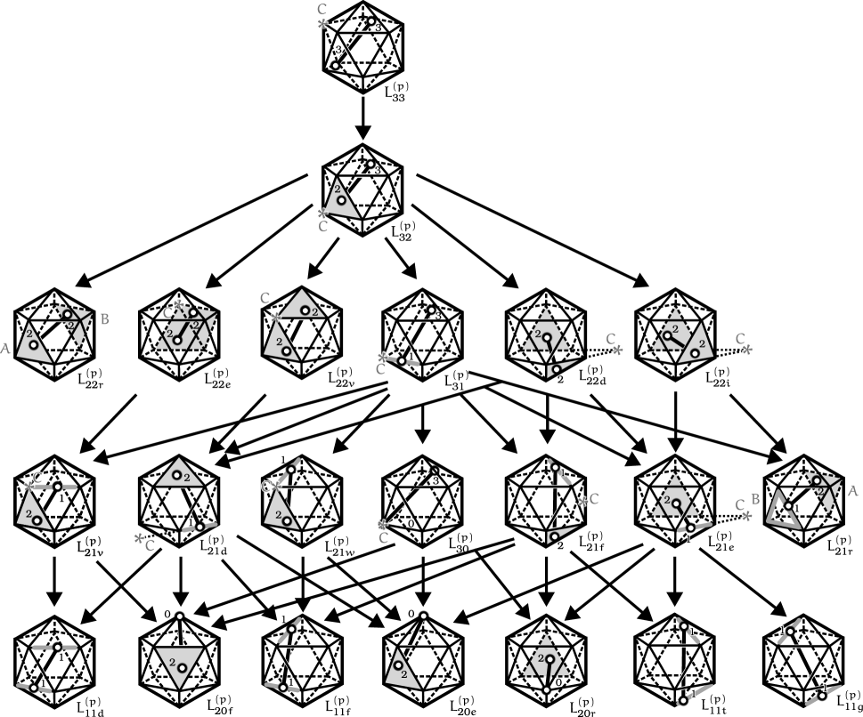
Figure 12: All different $L_{ab}^{(p)}$ configurations encountered for $K$ being a regular icosahedron

Performing the reduction, we get the set of equations:

$$pP_{33} =6(P_{32}-P_{33}),$$

$$pP_{32} =3(P_{22}-P_{32})+2(P_{31}-P_{32}),$$

$$pP_{31} =3(P_{21}-P_{31})+1(P_{30}-P_{31}),$$

$$pP_{22e} =4(P_{21v}-P_{22e}),$$

$$pP_{22v} =4(P_{21d}-P_{22v}),$$

$$pP_{22d} =4(P_{21}^{\prime}-P_{22d}),$$

$$pP_{22i} =4(P_{21}^{\prime\prime}-P_{22i}),$$

$$pP_{30} =3(P_{20}-P_{30}),$$

$$pP_{21v} =2(P_{11d}-P_{21v})+1(P_{20u}-P_{21v}),$$

$$pP_{21w} =2(P_{11f}-P_{21w})+1(P_{20l}-P_{21w}),$$

$$pP_{21f} =2(P_{11}-P_{21f})+1(P_{20}^{\prime}-P_{21f}),$$

$$pP_{21d} =2(P_{11}^{\prime}-P_{21d})+1(P_{20}^{\prime\prime}-P_{21d}),$$

$$pP_{21e} =2(P_{11}^{\prime\prime}-P_{21e})+1(P_{20}^{\prime\prime\prime}-P_{21e}),$$

with

$$P_{22} =\frac{2P_{22d}}{5}+\frac{P_{22r}}{10}+\frac{P_{22v}}{5}+\frac{P_{22e}}{10\phi^{2}}+\frac{\phi^{2}P_{22i}}{10},$$

$$P_{21} =\frac{\phi P_{21e}}{5}+\frac{P_{21f}}{2\phi\sqrt{5}}+\frac{P_{21r}}{5}+\frac{P_{21d}}{5}+\frac{P_{21v}}{5\phi^{2}}+\frac{P_{21w}}{10\phi},$$

$$P_{21}^{\prime} =\frac{P_{21f}}{2}-\frac{\phi P_{21d}}{2}+\frac{\phi^{2}P_{21e}}{2},$$

$$P_{21}^{\prime\prime} =\phi^{2}P_{21r}-\phi P_{21e},$$

$$P_{20} =\frac{P_{20f}}{2\phi^{2}}+\frac{P_{20e}}{2\phi}+\frac{P_{20r}}{2},$$

$$P_{20}^{\prime} =\phi P_{20r}-\frac{P_{20f}}{\phi},$$

$$P_{20}^{\prime\prime} =\phi^{2}P_{20e}-\phi P_{20f},$$

$$P_{20}^{\prime\prime\prime} =\phi^{2}P_{20r}-\phi P_{20e},$$

$$P_{11} =2P_{11t}-P_{11f},$$

$$P_{11}^{\prime} =\phi^{2}P_{11f}-\phi P_{11d},$$

$$P_{11}^{\prime\prime} =\phi^{2}P_{11g}-\phi P_{11t}.$$

Solving the system, we get, after simplifications,

$$\begin{split}P_{33}&=\frac{18\left(12\phi^{2}P_{11d}-12\phi^{4}P_{11f}+4\phi^{8}P_{11g}+12\phi^{2}P_{11t}-6\phi^{4}P_{20e}+4\phi^{8}P_{20r}+6P_{20f}\right)}{5\phi^{4}(3+p)(4+p)(5+p)(6+p)}\\ &+\frac{108\phi^{2}P_{21r}}{5(4+p)(5+p)(6+p)}+\frac{9P_{22r}}{5(5+p)(6+p)}.\end{split}$$ (83)

When $p=1$, we get for the mean distance

$$\begin{split}L_{33}&=\frac{3L_{22r}}{70}-\frac{9L_{11f}}{175}-\frac{9L_{20e}}{350}+\frac{9L_{20f}}{350\phi^{4}}+\frac{9L_{11d}}{175\phi^{2}}+\frac{9L_{11t}}{175\phi^{2}}+\frac{18\phi^{2}L_{21r}}{175}+\frac{3\phi^{4}L_{11g}}{175}+\frac{3\phi^{4}L_{20r}}{175}.\end{split}$$ (84)

5.4.1 L_11d

Let $A^{\prime}=\overline{[1,0,\phi][-1,0,\phi]}$ and $B^{\prime}=\overline{[0,\phi,1][\phi,1,0]}$ be edges of $K$, then $L_{11d}=L_{A^{\prime}B^{\prime}}$. By shifting, $L_{A^{\prime}B^{\prime}}=L_{OA}$, where $O=[0,0,0]$ is the origin and $A=A^{\prime}-B^{\prime}$ is a polygon with vertices $[1,-\phi,\frac{1}{\phi}],[-\frac{1}{\phi},-1,\phi],[-\phi^{2},-1,\phi],[-1,-\phi,\frac{1}{\phi}]$ (a parallelogram) having area $\operatorname{vol}A=\sqrt{10-2\sqrt{5}}$. Projecting $O$ onto $\mathcal{A}(A)$, we obtain $\operatorname{proj}_{A}O=[0,-1-\frac{1}{\sqrt{5}},\frac{2}{\sqrt{5}}]$ and separation $h=\sqrt{2+\frac{2}{\sqrt{5}}}$. Point-Polygon formula yields

$$\begin{split}L_{11d}=\frac{2h^{3}}{\operatorname{vol}A}\Bigg{(}&2I^{(1)}_{00}\left(\frac{1}{2\phi^{2}},\frac{2\pi}{5}\right)-I^{(1)}_{00}\left(\frac{1}{2},\frac{\pi}{5}\right)+I^{(1)}_{00}\left(\frac{1}{2},\frac{2\pi}{5}\right)\Bigg{)}\approx 2.0431430525135.\end{split}$$ (85)

Explicitly, after series of simplifications on $I^{(1)}_{00}(\cdot,\cdot)$ by recursion formulae, we obtain

$$\begin{split}L_{11d}&=\frac{5}{6}+\frac{1}{2\sqrt{5}}+\frac{1}{15}(2\pi)\left(3+\sqrt{5}\right)-\frac{8}{15}\left(3+\sqrt{5}\right)\operatorname{arccot}\phi\\ &-\frac{8}{15}\left(3+\sqrt{5}\right)\operatorname{arccot}\left(\phi^{2}\right)+\frac{1}{60}\left(31-3\sqrt{5}\right)\ln 3+\frac{13}{120}\left(3+\sqrt{5}\right)\ln 5.\end{split}$$ (86)

5.4.2 L_11g

Let $A^{\prime}$ be the same edge as in $L_{11d}$ and $B^{\prime}=\overline{[1,0,\phi][-1,0,\phi]}$, then $L_{11g}=L_{A^{\prime}B^{\prime}}$. By shifting, $L_{A^{\prime}B^{\prime}}=L_{OA}$, where $O=[0,0,0]$ and $A=A^{\prime}-B^{\prime}$ is a polygon with vertices $[0,0,2\phi],[1,-\phi,\phi^{2}],[-1,-\phi,\phi^{2}],[-2,0,2\phi]$ having area $\operatorname{vol}A=2\sqrt{3}$. Projecting $O$ onto $\mathcal{A}(A)$, we obtain $\operatorname{proj}_{A}O=[0,-\frac{2\phi}{3},\frac{2\phi^{3}}{3}]$ and separation $h=\sqrt{\frac{14}{3}+2\sqrt{5}}$. Point-Polygon formula yields

$$\begin{split}L_{11g}=\frac{2h^{3}}{\operatorname{vol}A}\Bigg{(}&2I^{(1)}_{00}\left(\frac{1}{2\phi^{2}},\frac{\pi}{3}\right)+I^{(1)}_{00}\left(\frac{1}{\phi^{2}},\frac{\pi}{3}\right)\Bigg{)}\approx 3.1806727116118.\end{split}$$ (87)

Explicitly, after series of simplifications,

$$\begin{split}L_{11g}&=\frac{1}{9}+\frac{\sqrt{5}}{9}+\frac{2}{9}\sqrt{2\left(5+\sqrt{5}\right)}+\frac{4}{45}\left(9+4\sqrt{5}\right)\pi-\frac{16}{27}\left(9+4\sqrt{5}\right)\operatorname{arccot}\phi\\ &+\left(\frac{43}{27}+\frac{2\sqrt{5}}{3}\right)\operatorname{arccoth}\phi+\frac{2}{27}\left(23+9\sqrt{5}\right)\operatorname{arccsch}\phi-\left(\frac{43}{108}+\frac{\sqrt{5}}{6}\right)\ln 5.\end{split}$$ (88)

5.4.3 L_11f

Let $A^{\prime}$ be the same edge as in $L_{11d}$ and $B^{\prime}=\overline{[\phi,1,0][\phi,-1,0]}$, then $L_{11f}=L_{A^{\prime}B^{\prime}}$. By shifting, $L_{A^{\prime}B^{\prime}}=L_{OA}$, where $O=[0,0,0]$ and $A=A^{\prime}-B^{\prime}$ is a polygon with vertices $[-\frac{1}{\phi},-1,\phi],[-\frac{1}{\phi},1,\phi],[-\phi^{2},1,\phi],[-\phi^{2},-1,\phi]$ having area $\operatorname{vol}A=4$. Projecting $O$ onto $\mathcal{A}(A)$, we obtain $\operatorname{proj}_{A}O=[0,0,\phi]$ and separation $h=\phi$. Point-Polygon formula yields

$$\begin{split}L_{11f}=\frac{2h^{3}}{\operatorname{vol}A}\Bigg{(}&I^{(1)}_{00}\left(\frac{1}{\phi},\arctan\left(\phi^{2}\right)\right)+I^{(1)}_{00}\left(\phi,\arctan\left(\frac{1}{\phi^{2}}\right)\right)-I^{(1)}_{00}\left(\frac{1}{\phi^{2}},\arctan\phi\right)\\ &-I^{(1)}_{00}\left(\frac{1}{\phi},\arctan\frac{1}{\phi}\right)\Bigg{)}\approx 2.3977565034445.\end{split}$$ (89)

Explicitly, after series of simplifications,

$$\begin{split}L_{11f}&=\frac{5}{6}+\frac{\sqrt{5}}{6}-\frac{\pi}{96}\left(1+\sqrt{5}\right)^{3}+\frac{1}{2}\left(2+\sqrt{5}\right)\operatorname{arccot}\phi-\frac{1}{6}\left(2+\sqrt{5}\right)\operatorname{arccot}\left(\phi^{2}\right)\\ &+\frac{1}{24}\left(39+17\sqrt{5}\right)\operatorname{arccoth}\phi+\frac{1}{48}\left(1-5\sqrt{5}\right)\ln 3-\frac{1}{96}\left(17+11\sqrt{5}\right)\ln 5.\end{split}$$ (90)

5.4.4 L_11t

Again, let $A^{\prime}$ be the same edge as in $L_{11d}$ and $B^{\prime}=\overline{[1,0,-\phi][\phi,1,0]}$, then $L_{11t}=L_{A^{\prime}B^{\prime}}$. By shifting, $L_{A^{\prime}B^{\prime}}=L_{OA}$, where $O=[0,0,0]$ and $A=A^{\prime}-B^{\prime}$ is a polygon with vertices $[0,0,2\phi],[-\frac{1}{\phi},-1,\phi],[-\phi^{2},-1,\phi],[-2,0,2\phi]$ having area $\operatorname{vol}A=\sqrt{2\left(5+\sqrt{5}\right)}$. Projecting $O$ onto $\mathcal{A}(A)$, we obtain $\operatorname{proj}_{A}O=[0,-1-\frac{1}{\sqrt{5}},\frac{2}{\sqrt{5}}]$ and separation $h=\sqrt{2+\frac{2}{\sqrt{5}}}$. Point-Polygon formula yields

$$L_{11t}=\frac{2h^{3}}{\operatorname{vol}A}\Bigg{(}I^{(1)}_{00}\left(\frac{1}{2},\frac{\pi}{5}\right)-I^{(1)}_{00}\left(\frac{1}{2},\frac{2\pi}{5}\right)+I^{(1)}_{00}\left(\phi,\frac{\pi}{5}\right)\Bigg{)}\approx 2.8940519649490.$$ (91)

Explicitly, after series of simplifications,

$$\begin{split}L_{11t}&=\frac{4}{3}\sqrt{1+\frac{2}{\sqrt{5}}}-\frac{1}{6}-\frac{\sqrt{5}}{6}-\frac{8\pi}{75}\left(1+\sqrt{5}\right)+\frac{8}{15}\left(1+\sqrt{5}\right)\operatorname{arccot}\phi\\ &+\frac{4}{15}\left(8+3\sqrt{5}\right)\operatorname{arccsch}\phi-\frac{13}{120}\left(1+\sqrt{5}\right)\ln 5.\end{split}$$ (92)

5.4.5 L_20e

Let $A$ be the face of $K$ with vertices $[1,0,\phi]$, $[-1,0,\phi]$, $[0,\phi,1]$ (an equilateral triangle) and let $B$ be vertex $[\phi,-1,0]$, then $L_{20e}=L_{AB}$. Projecting $B$ onto $\mathcal{A}(A)$, we obtain $\operatorname{proj}_{A}B=[\phi,-\frac{1}{3},\frac{2\phi^{2}}{3}]$ and separation $h=2\phi/\sqrt{3}$. By Point-Polygon formula,

$$\begin{split}L_{20e}=\frac{2h^{3}}{\nu}\Bigg{(}&I^{(1)}_{00}\left(\frac{1}{2\phi^{2}},\frac{\pi}{3}\right)-I^{(1)}_{00}\left(\frac{1}{2\phi^{2}},\arctan\left(\sqrt{15}+2\sqrt{3}\right)\right)\\ &+I^{(1)}_{00}\left(\frac{\phi^{2}}{2},\arctan\left(\sqrt{15}-2\sqrt{3}\right)\right)\Bigg{)}\approx 2.688729552544.\end{split}$$ (93)

Explicitly, after series of simplifications,

$$\begin{split}L_{20e}&=\frac{7}{9}+\frac{\sqrt{5}}{9}+\frac{8\pi}{27}\left(2+\sqrt{5}\right)-\frac{16}{9}\left(2+\sqrt{5}\right)\operatorname{arccot}\phi\\ &+\frac{1}{27}\left(104+47\sqrt{5}\right)\operatorname{arccoth}\phi-\frac{1}{108}\left(112+61\sqrt{5}\right)\ln 5.\end{split}$$ (94)

5.4.6 L_20r

Let $A$ be the same face of $K$ as in the section on $L_{20e}$ and let $B$ be vertex $[1,0,-\phi]$, then $L_{20r}=L_{AB}$. Projecting $B$ onto $\mathcal{A}(A)$, we obtain $\operatorname{proj}_{A}B=[1,\frac{2\phi}{3},\frac{\sqrt{5}\phi}{3}]$ and separation $h=2\phi^{2}/\sqrt{3}$. By Point-Polygon formula,

$$L_{20r}=\frac{2h^{3}}{\nu}\Bigg{(}I^{(1)}_{00}\left(\frac{1}{\phi^{2}},\frac{\pi}{3}\right)-I^{(1)}_{00}\left(\frac{1}{2\phi^{2}},\frac{\pi}{3}\right)\Bigg{)}\approx 3.28394367574.$$ (95)

Explicitly, after series of simplifications,

$$\begin{split}L_{20r}&=\frac{4}{9}\sqrt{2\left(5+\sqrt{5}\right)}-\frac{1}{9}-\frac{\sqrt{5}}{9}-\frac{16\pi}{135}\left(9+4\sqrt{5}\right)+\frac{16}{27}\left(9+4\sqrt{5}\right)\operatorname{arccot}\phi\\ &-\left(\frac{43}{27}+\frac{2\sqrt{5}}{3}\right)\operatorname{arccoth}\phi+\frac{4}{27}\left(23+9\sqrt{5}\right)\operatorname{arccsch}\phi+\left(\frac{43}{108}+\frac{\sqrt{5}}{6}\right)\ln 5.\end{split}$$ (96)

5.4.7 L_20f

Let $A$ be the same face of $K$ as in the section on $L_{20e}$ and let $B$ be vertex $[\phi,1,0]$, then $L_{20f}=L_{AB}$. Projecting $B$ onto $\mathcal{A}(A)$, we obtain $\operatorname{proj}_{A}B=[\phi,\frac{\phi^{3}}{3},\frac{2\phi}{3}]$ and separation $h=2/\sqrt{3}$. By Point-Polygon formula,

$$\begin{split}L_{20f}=\frac{2h^{3}}{\nu}\Bigg{(}&I^{(1)}_{00}\left(\frac{\phi^{2}}{2},\frac{\pi}{3}\right)-I^{(1)}_{00}\left(\frac{\sqrt{5}}{2},\arctan\sqrt{\frac{3}{5}}\right)\\ &-I^{(1)}_{00}\left(\frac{\phi^{2}}{2},\arctan\left(\sqrt{15}-2\sqrt{3}\right)\right)\Bigg{)}\approx 2.2472771159735.\end{split}$$ (97)

Explicitly, after series of simplifications,

$$L_{20f}=\frac{10}{9}+\frac{2\sqrt{5}}{9}-\frac{8\pi}{27}+\frac{32}{27}\operatorname{arccot}\phi+\frac{16}{27}\operatorname{arccot}(\phi^{2})-\frac{17}{54}\sqrt{5}\ln 3+\left(\frac{1}{2}+\frac{5\sqrt{5}}{27}\right)\ln 5.$$ (98)

5.4.8 L_21r

Let $A$ be a face of $K$ and $B$ be a boundary of the opposite face. In icosahedron $K$, two faces are separated by the distance $2\phi^{2}/\sqrt{3}$. Since the overlap diagram of these faces is the same as the one associated to two opposite faces of an octahedron (see Figure 10), the coefficients of the expansion of irreducible $L_{21r}$ term into auxiliary integrals $I^{(1)}_{ij}$ match. However, this is only valid provided the edge length is $\sqrt{2}$. Since our icosahedron $K$ has $l=2$, we first rescale our icosahedron by $1/\sqrt{2}$. In the final step, since the mean distance scales linearly, we have just rescale $L_{ab}$ back by multiplying it by $\sqrt{2}$. Hence, by using Equation (74),

$$\begin{split}L_{21r}&=L_{21r}\big{|}_{l=2}=\sqrt{2}L_{21r}\big{|}_{l=\sqrt{2}}=\sqrt{2}\frac{6h^{3}}{\operatorname{vol}A\operatorname{vol}B}\Bigg{[}\frac{4\sqrt{2}}{3}I^{(1)}_{00}\left(\frac{\sqrt{6}}{3h},\frac{\pi}{3}\right)-\frac{h}{\sqrt{3}}I^{(1)}_{10}\left(\frac{\sqrt{6}}{3h},\frac{\pi}{3}\right)\\ &-hI^{(1)}_{01}\left(\frac{\sqrt{6}}{3h},\frac{\pi}{3}\right)+\frac{2h}{\sqrt{3}}I^{(1)}_{10}\left(\frac{\sqrt{6}}{6h},\frac{\pi}{3}\right)-\frac{\sqrt{2}}{3}I^{(1)}_{00}\left(\frac{\sqrt{6}}{6h},\frac{\pi}{3}\right)\Bigg{]}\approx 3.1819213671057,\end{split}$$ (99)

where $h=\sqrt{2}\phi^{2}/\sqrt{3}$, $\operatorname{vol}A=\sqrt{3}/2$ and $\operatorname{vol}B=3\sqrt{2}$ are the rescaled icosahedron opposite faces separation, rescaled face area and face perimeter, respectively. Contrary to the octahedron case, we now have $\frac{\sqrt{6}}{3h}=1/\phi^{2}$ and $\frac{\sqrt{6}}{6h}=1/(2\phi^{2})$. Via recursions, we get after some simplifications,

$$\begin{split}L_{21r}&=\frac{227}{108}+\frac{107\sqrt{5}}{108}-\frac{25}{27}\sqrt{10+\frac{22}{\sqrt{5}}}-\frac{8\pi}{135}\left(9+4\sqrt{5}\right)+\frac{16}{81}\left(9+4\sqrt{5}\right)\operatorname{arccot}\phi\\ &+\left(\frac{1043}{324}+\frac{13\sqrt{5}}{9}\right)\operatorname{arccoth}\phi+\left(\frac{179}{81}+\frac{7\sqrt{5}}{9}\right)\operatorname{arccsch}\phi-\frac{1043+468\sqrt{5}}{1296}\ln 5.\end{split}$$ (100)

5.4.9 L_22r

Again, Overlap diagram of $L_{21r}$ configuration matches that of an octahedron. Immediately from Equation (79), by rescaling and replacing $\sqrt{2}/2$ by $1/\phi^{2}$ and $\sqrt{2}/4$ by $1/(2\phi^{2})$ in the first argument of $I^{(p)}_{ij}$ integrals, we get

$$\begin{split}L_{22r}&=\sqrt{2}\frac{6h^{3}}{\operatorname{vol}A\operatorname{vol}B}\Bigg{[}\frac{4}{3\sqrt{3}}I^{(1)}_{00}\left(\frac{1}{\phi^{2}},\frac{\pi}{3}\right)-\frac{\sqrt{2}h}{3}I^{(1)}_{10}\left(\frac{1}{\phi^{2}},\frac{\pi}{3}\right)-\sqrt{\frac{2}{3}}hI^{(1)}_{01}\left(\frac{1}{\phi^{2}},\frac{\pi}{3}\right)\\ &-\frac{h^{2}}{\sqrt{3}}I^{(1)}_{20}\left(\frac{1}{\phi^{2}},\frac{\pi}{3}\right)+h^{2}I^{(1)}_{11}\left(\frac{1}{\phi^{2}},\frac{\pi}{3}\right)-\frac{1}{3\sqrt{3}}I^{(1)}_{00}\left(\frac{1}{2\phi^{2}},\frac{\pi}{3}\right)+\frac{2\sqrt{2}h}{3}I^{(1)}_{10}\left(\frac{1}{2\phi^{2}},\frac{\pi}{3}\right)\\ &-\frac{2h^{2}}{\sqrt{3}}I^{(1)}_{20}\left(\frac{1}{2\phi^{2}},\frac{\pi}{3}\right)\Bigg{]}\approx 3.12998447304770,\end{split}$$ (101)

where $h=\sqrt{2}\phi^{2}/\sqrt{3}$ and $\operatorname{vol}A=\operatorname{vol}B=\sqrt{3}/2$. Explicitly, after some simplifications,

$$\begin{split}L_{22r}&=\frac{4}{9}\left(3+2\sqrt{5}\right)\sqrt{10+\frac{22}{\sqrt{5}}}-\frac{271}{45}-\frac{119}{9\sqrt{5}}+\frac{16\pi}{675}\left(78+35\sqrt{5}\right)-\frac{32}{135}\left(67+30\sqrt{5}\right)\operatorname{arccot}\phi\\ &+\left(\frac{611}{45}+\frac{164\sqrt{5}}{27}\right)\operatorname{arccoth}\phi-\frac{28}{135}\left(9+5\sqrt{5}\right)\operatorname{arccsch}\phi-\left(\frac{611}{180}+\frac{41\sqrt{5}}{27}\right)\ln 5.\end{split}$$ (102)

5.4.10 L₃₃

Putting everything together by using (84), we finally arrive at

$$\begin{split}L_{33}&=\frac{197}{525}+\frac{239}{525\sqrt{5}}-\frac{44}{525}\sqrt{2+\frac{2}{\sqrt{5}}}-\frac{\left(17226+6269\sqrt{5}\right)\pi}{157500}-\frac{\left(2186+1413\sqrt{5}\right)\operatorname{arccot}\phi}{15750}\\ &+\frac{\left(82-75\sqrt{5}\right)\operatorname{arccot}\left(\phi^{2}\right)}{5250}+\frac{\left(15969+7151\sqrt{5}\right)\operatorname{arccoth}\phi}{12600}+\frac{4\left(2139+881\sqrt{5}\right)\operatorname{arccsch}\phi}{7875}\\ &+\frac{\left(4449-1685\sqrt{5}\right)\ln 3}{42000}-\frac{\left(75783+37789\sqrt{5}\right)\ln 5}{252000}\approx 1.66353152568500.\end{split}$$ (103)

Rescaling, we get our mean distance in a regular icosahedron having unit volume

$$L_{33}\big{|}_{\operatorname{vol}K=1}=\frac{L_{33}}{\sqrt[3]{\frac{10}{3}\left(3+\sqrt{5}\right)}}\approx 0.64131248551.$$ (104)

5.5 Regular dodecahedron

Finaly, we will calculte the mean distance in the regular dodecahedron. Let us choose the vertices as $[\pm\phi,\pm\phi,\pm\phi],[0,\pm 1,\pm\phi^{2}]$ and all their cyclic permutations ($\phi=(1+\sqrt{5})/2$ as usual). Under this choice, each edge has length $l=2$ and each face has area $\nu=\sqrt{25+10\sqrt{5}}$.

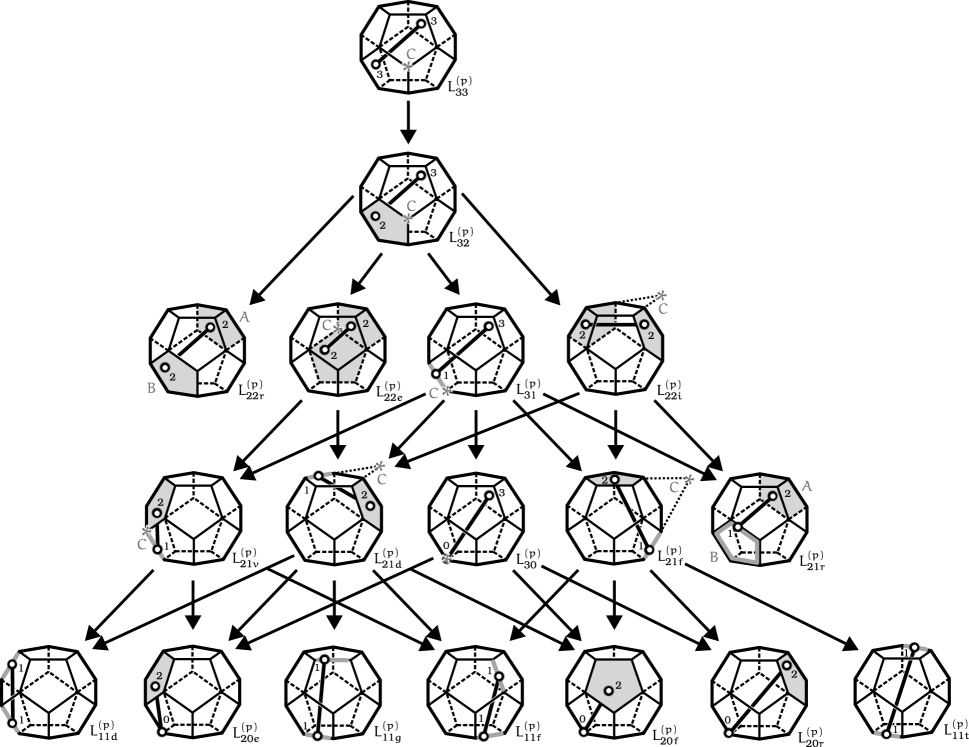
Figure 13: All different $L_{ab}^{(p)}$ configurations encountered for $K$ being a regular icosahedron

Performing CRT, we get the configurations shown in Figure 13. Even though there are less configurations than for the icosahedron, the dodecahedron has more complicated overlap diagram (see Figure 14, there is ten-fold symmetry with respect to rotation and reflection). Distance moments are again connected through CRT via the following set of reduction equations

$$pP_{33} =6(P_{32}-P_{33}),$$

$$pP_{32} =3(P_{22}-P_{32})+2(P_{31}-P_{32}),$$

$$pP_{31} =3(P_{21}-P_{31})+1(P_{30}-P_{31}),$$

$$pP_{22e} =4(P_{21}^{\prime}-P_{22e}),$$

$$pP_{22i} =4(P_{21}^{\prime\prime}-P_{22i}),$$

$$pP_{30} =3(P_{20}-P_{30}),$$

$$pP_{21v} =1(P_{20e}-P_{21v})+2(P_{11}-P_{21v}),$$

$$pP_{21f} =2(P_{11}^{\prime}-P_{21f})+1(P_{20}^{\prime}-P_{21f}),$$

$$pP_{21d} =2(P_{11}^{\prime\prime}-P_{21d})+1(P_{20}^{\prime\prime}-P_{21d})$$

with

$$P_{22} =\frac{1}{6\phi}\left(\sqrt{5}P_{22e}+\phi P_{22r}+\phi^{2}\sqrt{5}P_{22i}\right),$$

$$P_{21} =\frac{P_{21r}}{3}+\frac{P_{21d}}{3}+\frac{\phi P_{21f}}{6}+\frac{P_{21v}}{6\phi^{2}},$$

$$P_{21}^{\prime} =\frac{1}{\phi\sqrt{5}}\left(P_{21v}+\phi^{2}P_{21d}\right),$$

$$P_{21}^{\prime\prime} =\frac{1}{\sqrt{5}}\left(\phi P_{21f}+\phi P_{21r}-P_{21d}\right),$$

$$P_{20} =\frac{1}{2\phi^{2}}\left(P_{20e}+\phi P_{20f}+\phi^{2}P_{20r}\right),$$

$$P_{20}^{\prime} =\phi^{2}P_{20r}-\phi P_{20f},$$

$$P_{20}^{\prime\prime} =\phi^{2}P_{20f}-\phi P_{20e},$$

$$P_{11} =\frac{1}{\phi\sqrt{5}}\left(2P_{11d}+\phi P_{11f}\right),$$

$$P_{11}^{\prime} =\frac{1}{\sqrt{5}}\left(2\phi P_{11t}-P_{11f}\right),$$

$$P_{11}^{\prime\prime} =\frac{1}{\sqrt{5}}\left(\phi P_{11g}+\phi P_{11f}-P_{11d}\right).$$

Solving the system, we get, after simplifications,

$$\begin{split}P_{33}=\,&\frac{12\left(2\sqrt{5}P_{11d}+5\phi P_{20e}+2\phi^{3}P_{11g}-2\phi^{4}\sqrt{5}P_{11f}-5\phi^{5}P_{20f}+4\sqrt{5}\phi^{6}P_{20r}+2\phi^{9}P_{11t}\right)}{\phi^{4}\sqrt{5}\,(3+p)(4+p)(5+p)(6+p)}\\ &+\frac{60\phi P_{21r}}{\sqrt{5}(4+p)(5+p)(6+p)}+\frac{3P_{22r}}{(5+p)(6+p)}.\end{split}$$ (105)

When $p=1$, we get for the mean distance

$$L_{33}=\frac{L_{11d}}{35\phi^{4}}+\frac{L_{20e}}{14\sqrt{5}\phi^{3}}+\frac{L_{11g}}{35\sqrt{5}\phi}-\frac{L_{11f}}{35}+\frac{L_{22r}}{14}-\frac{\phi L_{20f}}{14\sqrt{5}}+\frac{2\phi L_{21r}}{7\sqrt{5}}+\frac{2\phi^{2}L_{20r}}{35}+\frac{\phi^{5}L_{11t}}{35\sqrt{5}}.$$ (106)

5.5.1 L_11d

Let $A^{\prime}=\overline{[0,\phi^{2},1][0,\phi^{2},-1]}$ and $B^{\prime}=\overline{[\phi,\phi,-\phi][1,0,-\phi^{2}]}$ be edges of $K$, then $L_{11d}=L_{A^{\prime}B^{\prime}}$. By shifting, $L_{A^{\prime}B^{\prime}}=L_{OA}$, where $O=[0,0,0]$ is the origin and $A=A^{\prime}-B^{\prime}$ is a polygon with vertices $[-\phi,1,\phi^{2}],[-1,\phi^{2},\sqrt{5}\phi],[-1,\phi^{2},\phi],[-\phi,1,1/\phi]$ having area $\operatorname{vol}A=2\sqrt{3}$. Projecting $O$ onto $\mathcal{A}(A)$, we obtain $\operatorname{proj}_{A}O=[-1-\frac{\sqrt{5}}{3},\frac{2}{3},0]$ and separation $h=(1+\sqrt{5})/\sqrt{3}$. Point-Polygon formula yields

$$\begin{split}L_{11d}=\frac{2h^{3}}{\operatorname{vol}A}\Bigg{(}&I^{(1)}_{00}\left(\frac{1}{2\phi^{2}},\frac{\pi}{3}\right)+I^{(1)}_{00}\left(\frac{\sqrt{5}}{2},\frac{\pi}{3}\right)-I^{(1)}_{00}\left(\frac{1}{2\phi^{2}},\arctan\left(\sqrt{3}\left(2+\sqrt{5}\right)\right)\right)\\ &-I^{(1)}_{00}\left(\frac{\sqrt{5}}{2},\arctan\sqrt{\frac{3}{5}}\right)\Bigg{)}\approx 3.1367199950978.\end{split}$$ (107)

Explicitly, after series of simplifications,

$$\begin{split}L_{11d}&=\frac{10\sqrt{2}}{9}-\frac{\sqrt{5}}{3}+\frac{5\sqrt{10}}{9}-\frac{5}{9}-\frac{2\pi}{27}\left(2+\sqrt{5}\right)-\frac{17}{108}\left(5+2\sqrt{5}\right)\ln 3-\frac{1}{108}\left(4+7\sqrt{5}\right)\ln 5\\ &+\frac{4}{27}\left(2+\sqrt{5}\right)\left(2\operatorname{arccot}2+2\operatorname{arccot}\sqrt{2}-\arccos\frac{2}{3}\right)+\frac{17}{108}\left(5+2\sqrt{5}\right)\operatorname{arccosh}\frac{13}{3}.\end{split}$$ (108)

5.5.2 L_11g

Let $A^{\prime}$ be the same edge as in $L_{11d}$ and $B^{\prime}=\overline{[\phi,-\phi,\phi][\phi^{2},-1,0]}$, then $L_{11g}=L_{A^{\prime}B^{\prime}}$. By shifting, $L_{A^{\prime}B^{\prime}}=L_{OA}$, where $O=[0,0,0]$ and $A=A^{\prime}-B^{\prime}$ is a polygon with vertices $[-\phi,\phi^{3},-1/\phi],[-\phi^{2},\sqrt{5}\phi,1],[-\phi^{2},\sqrt{5}\phi,-1],[-\phi,\phi^{3},-\phi^{2}]$ having area $\operatorname{vol}A=\sqrt{10-2\sqrt{5}}$. Projecting $O$ onto $\mathcal{A}(A)$, we obtain $\operatorname{proj}_{A}O=[-1-\frac{3}{\sqrt{5}},2+\frac{4}{\sqrt{5}},0]$ and separation $h=\sqrt{10+\frac{22}{\sqrt{5}}}$. Point-Polygon formula yields

$$\begin{split}L_{11g}=\frac{2h^{3}}{\operatorname{vol}A}\Bigg{(}&2I^{(1)}_{00}\left(\frac{1}{2\phi^{4}},\frac{2\pi}{5}\right)-I^{(1)}_{00}\left(\frac{1}{2\phi^{2}},\frac{\pi}{5}\right)+I^{(1)}_{00}\left(\frac{1}{2\phi^{2}},\frac{2\pi}{5}\right)\Bigg{)}\approx 4.60478605392525.\end{split}$$ (109)

Explicitly, after series of simplifications,

$$\begin{split}L_{11g}&=\frac{5}{6}-\frac{1}{3\sqrt{2}}+\frac{11}{6\sqrt{5}}+\frac{1}{\sqrt{10}}-\left(\frac{47}{5}+\frac{21}{\sqrt{5}}\right)\pi+\frac{1}{120}\left(219+97\sqrt{5}\right)\ln 3\\ &+\frac{2}{15}\left(47+21\sqrt{5}\right)\left(\arccos\frac{2}{3}+2\arccos\frac{1}{\sqrt{41}}+2\arccos\frac{3}{\sqrt{41}}-2\operatorname{arccot}\sqrt{2}\right)\\ &+\frac{1}{120}\left(219+97\sqrt{5}\right)\left(\operatorname{arccosh}\frac{7}{3}-\operatorname{arccosh}3\right)\\ &+\frac{1}{60}\left(91+33\sqrt{5}\right)\left(\operatorname{arccosh}\frac{9}{\sqrt{41}}-\operatorname{arccosh}\frac{7}{\sqrt{41}}\right).\end{split}$$ (110)

5.5.3 L_11f

Let $A^{\prime}$ be the same edge as in $L_{11d}$ and $B^{\prime}=\overline{[1,0,-\phi^{2}][-1,0,-\phi^{2}]}$, then $L_{11f}=L_{A^{\prime}B^{\prime}}$. By shifting, $L_{A^{\prime}B^{\prime}}=L_{OA}$, where $O=[0,0,0]$ and $A=A^{\prime}-B^{\prime}$ is a polygon with vertices $[-1,\phi^{2},\sqrt{5}\phi],[1,\phi^{2},\sqrt{5}\phi],[1,\phi^{2},\phi],[-1,\phi^{2},\phi]$ having area $\operatorname{vol}A=4$. Projecting $O$ onto $\mathcal{A}(A)$, we obtain $\operatorname{proj}_{A}O=[0,\phi^{2},0]$ and separation $h=\phi^{2}$. Point-Polygon formula yields

$$\begin{split}L_{11f}=\frac{2h^{3}}{\operatorname{vol}A}\Bigg{(}&I^{(1)}_{00}\left(\frac{1}{\phi^{2}},\arctan\sqrt{5}\phi\right)+I^{(1)}_{00}\left(\frac{\sqrt{5}}{\phi},\arctan\frac{1}{\sqrt{5}\phi}\right)-I^{(1)}_{00}\left(\frac{1}{\phi^{2}},\arctan\phi\right)\\ &-I^{(1)}_{00}\left(\frac{1}{\phi},\arctan\frac{1}{\phi}\right)\Bigg{)}\approx 3.770095521642.\end{split}$$ (111)

Explicitly, after series of simplifications,

$$\begin{split}L_{11f}&=\frac{5}{3\sqrt{2}}-\frac{1}{2}+\sqrt{\frac{5}{2}}-\frac{\sqrt{5}}{6}+\left(\frac{3}{8}+\frac{\sqrt{5}}{6}\right)\pi+\frac{1}{48}\left(125+53\sqrt{5}\right)\arccos\frac{9}{\sqrt{41}}\\ &+\left(\frac{3}{8}+\frac{\sqrt{5}}{6}\right)\left(2\arccos\frac{13}{3\sqrt{41}}+2\operatorname{arccot}2-\arccos\frac{1}{9}-2\arccos\frac{3}{5}-2\arccos\frac{1}{\sqrt{41}}\right)\\ &+\frac{1}{48}\left(23+9\sqrt{5}\right)\operatorname{arccosh}\frac{13}{3}-\frac{1}{48}\left(125+53\sqrt{5}\right)\operatorname{arccosh}\frac{7}{\sqrt{41}}\\ &-\frac{1}{48}\left(37+17\sqrt{5}\right)\operatorname{arcsinh}2-\frac{1}{48}\left(23+9\sqrt{5}\right)\log(3)+\frac{1}{96}\left(37+17\sqrt{5}\right)\ln 5.\end{split}$$ (112)

5.5.4 L_11t

Again, let $A^{\prime}$ be the same edge as in $L_{11d}$ and $B^{\prime}=\overline{[\phi,-\phi,-\phi][0,-\phi^{2},-1]}$, then $L_{11t}=L_{A^{\prime}B^{\prime}}$. By shifting, $L_{A^{\prime}B^{\prime}}=L_{OA}$, where $O=[0,0,0]$ and $A=A^{\prime}-B^{\prime}$ is a polygon with vertices $[-\phi,\phi^{3},\phi^{2}],[0,2\phi^{2},2],[0,2\phi^{2},0],[-\phi,\phi^{3},1/\phi]$ having area $\operatorname{vol}A=\sqrt{2\left(5+\sqrt{5}\right)}$. Projecting $O$ onto $\mathcal{A}(A)$, we obtain $\operatorname{proj}_{A}O=[-1-\frac{3}{\sqrt{5}},2+\frac{4}{\sqrt{5}},0]$ and separation $h=\sqrt{10+\frac{22}{\sqrt{5}}}$. Point-Polygon formula yields

$$L_{11t}=\frac{2h^{3}}{\operatorname{vol}A}\Bigg{(}I^{(1)}_{00}\left(\frac{1}{\phi},\frac{\pi}{5}\right)+I^{(1)}_{00}\left(\frac{1}{2\phi^{2}},\frac{\pi}{5}\right)-I^{(1)}_{00}\left(\frac{1}{2\phi^{2}},\frac{2\pi}{5}\right)\Bigg{)}\approx 5.04162416571318.$$ (113)

Explicitly, after series of simplifications,

$$\begin{split}L_{11t}&=\frac{\sqrt{\frac{2}{5}}}{3}-\frac{1}{2}+2\sqrt{\frac{3}{5}}+\frac{2}{\sqrt{3}}-\frac{7}{6\sqrt{5}}-\frac{\pi}{45}\left(29+13\sqrt{5}\right)\\ &+\frac{2}{15}\left(29+13\sqrt{5}\right)\left(2\operatorname{arccot}\sqrt{2}-\arccos\frac{2}{3}\right)+\left(\frac{61}{15}+\frac{9}{\sqrt{5}}\right)\left(\operatorname{arccosh}4-\operatorname{arccosh}2\right)\\ &+\frac{1}{120}\left(133+61\sqrt{5}\right)\left(\operatorname{arccosh}3-\operatorname{arccosh}\frac{7}{3}-\ln 3\right).\end{split}$$ (114)

5.5.5 L_20e

Let $A$ be the face of $K$ with vertices $[1,0,-\phi^{2}]$, $[\phi,\phi,-\phi]$, $[0,\phi^{2},-1]$, $[-\phi,\phi,-\phi]$, $[-1,0,-\phi^{2}]$ (a regular pentagon) and let $B$ be vertex $[0,\phi^{2},1]$, then $L_{20e}=L_{AB}$. Projecting $B$ onto $\mathcal{A}(A)$, we obtain $\operatorname{proj}_{A}B=[0,\frac{3}{\phi^{2}\sqrt{5}},-\frac{1}{\sqrt{5}}]$ and separation $h=\sqrt{2+\tfrac{2}{\sqrt{5}}}$. By Point-Polygon formula,

$$\begin{split}L_{20e}=\frac{2h^{3}}{\nu}\Bigg{(}&I^{(1)}_{00}\left(\frac{1}{2},\frac{\pi}{5}\right)-I^{(1)}_{00}\left(\frac{1}{2},\frac{2\pi}{5}\right)-I^{(1)}_{00}\left(\frac{\phi^{2}}{2},\frac{\pi}{5}\right)+I^{(1)}_{00}\left(\frac{3\phi}{4},\arctan\frac{\sqrt{5-2\sqrt{5}}}{3}\right)\\ &+I^{(1)}_{00}\left(\frac{\phi^{2}}{2},\arctan\sqrt{5\left(5-2\sqrt{5}\right)}\right)\Bigg{)}\approx 3.346942678627.\end{split}$$ (115)

Explicitly, after series of simplifications,

$$\begin{split}&L_{20e}=\frac{7\sqrt{\frac{2}{5}}}{3}+\frac{13\sqrt{2}}{15}-\frac{4}{15}-\frac{4}{3\sqrt{5}}+\frac{4\pi}{15\sqrt{5}}-\left(\frac{1}{3}+\frac{9}{10\sqrt{5}}\right)\ln 3-\frac{13\ln 5}{30\sqrt{5}}+\frac{8\arccos\frac{2}{3}}{15\sqrt{5}}\\ &+\left(\frac{1}{3}+\frac{9}{10\sqrt{5}}\right)\operatorname{arccosh}\frac{13}{3}-\frac{3}{50}\left(25+8\sqrt{5}\right)\operatorname{arccosh}\frac{7}{\sqrt{41}}+\frac{3}{50}\left(25+8\sqrt{5}\right)\operatorname{arccosh}\frac{9}{\sqrt{41}}\\ &-\frac{16\operatorname{arccot}2}{15\sqrt{5}}+\frac{8\arctan\frac{9\sqrt{2}}{17}}{15\sqrt{5}}-\frac{8\arctan\frac{5\sqrt{2}}{7}}{15\sqrt{5}}-\frac{8\arctan\frac{3\sqrt{10}}{19}}{15\sqrt{5}}-\frac{8\arctan\sqrt{10}}{15\sqrt{5}}.\end{split}$$ (116)

5.5.6 L_20r

Let $A$ be the same face of $K$ as in the section on $L_{20e}$ and let $B$ be vertex $[0,-\phi^{2},1]$, then $L_{20r}=L_{AB}$. Projecting $B$ onto $\mathcal{A}(A)$, we obtain $\operatorname{proj}_{A}B=[0,\frac{1}{10}\left(\sqrt{5}-5\right),-1-\frac{4}{\sqrt{5}}]$ and separation $h=\sqrt{10+\frac{22}{\sqrt{5}}}$. By Point-Polygon formula,

$$\begin{split}L_{20r}&=\frac{2h^{3}}{\nu}\Bigg{(}I^{(1)}_{00}\left(\frac{1}{\phi},\frac{\pi}{5}\right)+I^{(1)}_{00}\left(\frac{1}{2\phi^{2}},\frac{2\pi}{5}\right)-I^{(1)}_{00}\left(\frac{1}{2\phi^{2}},\frac{\pi}{5}\right)-I^{(1)}_{00}\left(\frac{1}{2\phi^{4}},\frac{2\pi}{5}\right)\Bigg{)}\\ &\approx 4.87605984948.\end{split}$$ (117)

Explicitly, after series of simplifications,

$$\begin{split}L_{20r}&=\frac{4}{15}-\frac{2\sqrt{2}}{15}+\frac{4}{5\sqrt{3}}+\frac{2}{3\sqrt{5}}+\frac{4}{\sqrt{15}}+\frac{16\pi}{9}+\frac{4\pi}{\sqrt{5}}-\frac{16}{75}\left(20+9\sqrt{5}\right)\operatorname{arccot}\sqrt{2}\\ &+\left(\frac{3}{5}+\frac{43}{30\sqrt{5}}\right)\ln 3+\frac{8}{75}\left(20+9\sqrt{5}\right)\left(\arccos\frac{2}{3}-\arccos\frac{1}{\sqrt{41}}-\arccos\frac{3}{\sqrt{41}}\right)\\ &-\frac{2}{75}\left(85+37\sqrt{5}\right)\operatorname{arccosh}2+\left(\frac{3}{5}+\frac{43}{30\sqrt{5}}\right)\left(\operatorname{arccosh}\frac{7}{3}-\operatorname{arccosh}3\right)\\ &+\frac{2}{75}\left(85+37\sqrt{5}\right)\operatorname{arccosh}4+\left(\frac{1}{15}+\frac{9}{10\sqrt{5}}\right)\left(\operatorname{arccosh}\frac{7}{\sqrt{41}}-\operatorname{arccosh}\frac{9}{\sqrt{41}}\right)\end{split}$$ (118)

5.5.7 L_20f

Let $A$ be the same face of $K$ as in the section on $L_{20e}$ and let $B$ be vertex $[0,-\phi^{2},-1]$, then $L_{20f}=L_{AB}$. Projecting $B$ onto $\mathcal{A}(A)$, we obtain $\operatorname{proj}_{A}B=[0,-\frac{5+3\sqrt{5}}{10},-2-\frac{3}{\sqrt{5}}]$ and separation $h=2\sqrt{1+\frac{2}{\sqrt{5}}}$. By Point-Polygon formula,

$$\begin{split}L_{20f}=\frac{2h^{3}}{\nu}\Bigg{(}&I^{(1)}_{00}\left(\frac{\phi^{2}}{2},\frac{\pi}{5}\right)-I^{(1)}_{00}\left(\frac{1}{2\phi^{2}},\frac{2\pi}{5}\right)+I^{(1)}_{00}\left(\frac{1}{2\phi^{2}},\arctan\sqrt{5\left(5+2\sqrt{5}\right)}\right)\\ &-I^{(1)}_{00}\left(\frac{1}{2},\frac{\pi}{5}\right)-I^{(1)}_{00}\left(\frac{\phi^{2}}{2},\arctan\sqrt{85-38\sqrt{5}}\right)\Bigg{)}\approx 4.000363965317.\end{split}$$ (119)

Explicitly, after series of simplifications,

$$\begin{split}L_{20f}&=1+\frac{\sqrt{\frac{2}{5}}}{3}-\frac{\sqrt{2}}{5}+\frac{7}{3\sqrt{5}}+\frac{4\pi}{15}+\frac{8\pi}{15\sqrt{5}}+\frac{2}{3}\left(2+\sqrt{5}\right)\ln 3+\frac{13}{300}\left(5+2\sqrt{5}\right)\ln 5\\ &-\frac{16}{75}\left(5+2\sqrt{5}\right)\arccos\frac{2}{3}+\frac{8}{75}\left(5+2\sqrt{5}\right)\left(\operatorname{arccot}2+\arctan\frac{5\sqrt{2}}{7}-\arctan\left(7\sqrt{2}\right)\right)\\ &+\left(\frac{47}{30}+\frac{52}{15\sqrt{5}}\right)\operatorname{arccosh}\frac{7}{3}-\left(\frac{47}{30}+\frac{52}{15\sqrt{5}}\right)\operatorname{arccosh}3+\frac{1}{150}\left(35+4\sqrt{5}\right)\operatorname{arccosh}\frac{13}{3}\\ &-\frac{13}{150}\left(5+2\sqrt{5}\right)\operatorname{arcsinh}2.\end{split}$$ (120)

5.5.8 L_22r

Finally, let us take a closer look on parallel configurations $L_{21r}$ and $L_{22r}$. We start with the latter. Let $A$ and $B$ be opposite faces of dodecahedron $K$ with separation $h=\sqrt{10+\frac{22}{\sqrt{5}}}$ then $L_{22}=L_{AB}$ with overlap diagram as seen in Figure 14. Note that, due to symmetry, only one tenth of the diagram is sufficient to be considered. The subdomains where $\operatorname{vol}(A\cap\operatorname{proj}B+k)$ can be written as a single polynomial are shown in the diagram. Again, they are labeled by number of sides of polygon of intersection $A\cap(\operatorname{proj}B+k)$, sliding $\operatorname{proj}B+k$ across $\operatorname{proj}A$ by letting $k$ to vary (vector $k$ is shown by a black dot). Let us denote $D$ as the union of the labeled subdomains. Then, by Overlap formula,

$$L_{22r}=\frac{10}{\operatorname{vol}A\operatorname{vol}B}\int_{D}\sqrt{h^{2}+k^{2}}\operatorname{vol}(A\cap\operatorname{proj}B+k)\,\,\mathrm{d}k,$$ (121)

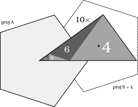
Figure 14: Overlap diagram for opposite-faces configuration in dodecahedron

Let us express $\operatorname{vol}(A\cap\operatorname{proj}B+k)$ in the aforementioned subdomains. We denote $v_{j}=\operatorname{vol}(A\cap\operatorname{proj}B+k)$ for all $k\in D_{j}$. Let us restrict ourselves to the plane $\mathcal{A}(A)$, in which we put $k=(x,y)$ and in which $\operatorname{proj}A$ is a regular pentagon with vertices $\left[\sqrt{2+\frac{2}{\sqrt{5}}}\cos\frac{2\pi i}{5},\sqrt{2+\frac{2}{\sqrt{5}}}\sin\frac{2\pi i}{5}\right]$, $i\in\{0,1,2,3,4\}$ and area $\operatorname{vol}A=\sqrt{5\left(5+2\sqrt{5}\right)}$. Similarly, $\operatorname{proj}B$ is another pentagon with vertices $\left[\sqrt{2+\frac{2}{\sqrt{5}}}\cos\frac{2\pi(i+1/2)}{5},\sqrt{2+\frac{2}{\sqrt{5}}}\sin\frac{2\pi(i+1/2)}{5}\right]$ and area $\operatorname{vol}B=\operatorname{vol}A=\sqrt{5\left(5+2\sqrt{5}\right)}$. Under this projection, the labeled subdomains $D_{j}$ are triangles with vertices

• (subdomain $D_{4}$) $\left[\sqrt{\frac{5}{2}+\frac{11}{2\sqrt{5}}},\frac{1}{2}\left(1+\sqrt{5}\right)\right],\left[\sqrt{2-\frac{2}{\sqrt{5}}},0\right],\left[\sqrt{8+\frac{8}{\sqrt{5}}},0\right]$, in which

  $$v_{4}=\frac{1}{10}\left(8\sqrt{50+22\sqrt{5}}-4\left(5+3\sqrt{5}\right)x+\sqrt{5\left(5+2\sqrt{5}\right)}x^{2}-5\sqrt{5-2\sqrt{5}}y^{2}\right),$$ (122)

• (subdomain $D_{6}$) $\left[\sqrt{\frac{5}{2}+\frac{11}{2\sqrt{5}}},\frac{1}{2}\left(1+\sqrt{5}\right)\right],\left[\sqrt{1-\frac{2}{\sqrt{5}}},\sqrt{5}-2\right],\left[\sqrt{2-\frac{2}{\sqrt{5}}},0\right]$, in which

  $$\begin{split}v_{6}&=\frac{1}{20}\bigg{(}8\sqrt{145+62\sqrt{5}}-4\left(5+3\sqrt{5}\right)x-\sqrt{10\left(5+\sqrt{5}\right)}x^{2}\\ &-4\sqrt{10\left(5+\sqrt{5}\right)}y+10\left(1+\sqrt{5}\right)xy-5\sqrt{2\left(5+\sqrt{5}\right)}y^{2}\bigg{)},\end{split}$$ (123)

• (subdomain $D_{8}$) $\left[\sqrt{1-\frac{2}{\sqrt{5}}},\sqrt{5}-2\right],\left[\sqrt{1-\frac{2}{\sqrt{5}}},0\right],\left[\sqrt{2-\frac{2}{\sqrt{5}}},0\right]$, in which

  $$v_{8}=\frac{1}{10}\left(4\sqrt{130+58\sqrt{5}}-8\sqrt{5}x-5\sqrt{1+\frac{2}{\sqrt{5}}}x^{2}-5\sqrt{5\left(5+2\sqrt{5}\right)}y^{2}\right),$$ (124)

• (subdomain $D_{10}$) $\left[\sqrt{1-\frac{2}{\sqrt{5}}},\sqrt{5}-2\right],\left[0,0\right],\left[\sqrt{1-\frac{2}{\sqrt{5}}},0\right]$, in which

  $$v_{10}=\frac{1}{2}\sqrt{5+2\sqrt{5}}\left(4-\sqrt{5}x^{2}-\sqrt{5}y^{2}\right).$$ (125)

In order to use the Overlap formula effectively, that is, to integrate $v_{j}=\operatorname{vol}(A\cap\operatorname{proj}B+k)$, $k\in D_{j}$ over all subdomains $D_{j}$, it is convenient to first perform appropriate rotation transformations and inclusion/exclusions. First, by inclusion/exclusion,

$$\begin{split}L_{22r}&=\frac{10}{\operatorname{vol}A\operatorname{vol}B}\bigg{(}\int_{D_{10}}u_{10}\sqrt{h^{2}+x^{2}+y^{2}}\,\,\mathrm{d}x\mathrm{d}y+\int_{D_{10}\cup D_{8}}u_{8}\sqrt{h^{2}+x^{2}+y^{2}}\,\,\mathrm{d}x\mathrm{d}y\\ &+\int_{D_{10}\cup D_{8}\cup D_{6}}u_{6}\sqrt{h^{2}+x^{2}+y^{2}}\,\,\mathrm{d}x\mathrm{d}y+\int_{D_{10}\cup D_{8}\cup D_{6}\cup D_{4}}u_{4}\sqrt{h^{2}+x^{2}+y^{2}}\,\,\mathrm{d}x\mathrm{d}y\bigg{)},\end{split}$$ (126)

where $u_{4}=v_{4}$, $u_{6}=v_{6}-v_{4}$, $u_{8}=v_{8}-v_{6}$ and $u_{10}=v_{10}-v_{8}$. Explicitly

$$u_{4}= \frac{4\sqrt{2}}{5}\sqrt{25+11\sqrt{5}}-\frac{2x}{5}\left(5+3\sqrt{5}\right)+\frac{x^{2}}{10}\sqrt{5\left(5+2\sqrt{5}\right)}-\frac{y^{2}}{2}\sqrt{5-2\sqrt{5}},$$ (127)

$$\begin{split}u_{6}=&-\frac{2}{5}\sqrt{5+2\sqrt{5}}+x\left(1+\frac{3}{\sqrt{5}}\right)-y\sqrt{2+\frac{2}{\sqrt{5}}}+\frac{xy}{2}\left(1+\sqrt{5}\right)\\ &-\frac{x^{2}\sqrt{2}}{4}\sqrt{5+\frac{11}{\sqrt{5}}}-\frac{y^{2}\sqrt{2}}{4}\sqrt{5-\sqrt{5}},\end{split}$$ (128)

$$u_{8}= -\frac{2}{5}\sqrt{5-2\sqrt{5}}+x\left(1-\frac{1}{\sqrt{5}}\right)+y\sqrt{2+\frac{2}{\sqrt{5}}}-\frac{xy}{2}\left(1+\sqrt{5}\right)$$ (129)

$$-\frac{x^{2}\sqrt{2}}{4}\sqrt{1-\frac{1}{\sqrt{5}}}-\frac{y^{2}\sqrt{2}}{4}\sqrt{25+11\sqrt{5}},$$ (130)

$$\begin{split}u_{10}=&-\frac{2}{5}\sqrt{5-2\sqrt{5}}+\frac{4x}{\sqrt{5}}-2x^{2}\sqrt{1+\frac{2}{\sqrt{5}}}.\end{split}$$ (131)

Note that domain $D_{10}$ is already in the form of the fundamental triangle domain $D\left(\zeta,\frac{\pi}{5}\right)$ with $\zeta=\sqrt{1-\frac{2}{\sqrt{5}}}$. Since $\zeta/h=1/(2\phi^{4})$, we immediately get in terms of auxiliary integrals,

$$\begin{split}\int_{D_{10}}u_{10}\sqrt{h^{2}+x^{2}+y^{2}}\,\,\mathrm{d}x\mathrm{d}y=h^{3}\Bigg{(}&-\frac{2}{5}\sqrt{5-2\sqrt{5}}I^{(1)}_{00}\left(\frac{1}{2\phi^{4}},\frac{\pi}{5}\right)+\frac{4h}{\sqrt{5}}I^{(1)}_{10}\left(\frac{1}{2\phi^{4}},\frac{\pi}{5}\right)\\ &-2h^{2}\sqrt{1+\frac{2}{\sqrt{5}}}I^{(1)}_{20}\left(\frac{1}{2\phi^{4}},\frac{\pi}{5}\right)\Bigg{)}.\end{split}$$ (132)

Domain $D=D_{10}\cup D_{8}\cup D_{6}\cup D_{4}$ in $(x,y)$ is transformed to the fundamental domain $D(\zeta,\frac{\pi}{5})$ with $\zeta=2\sqrt{1+\frac{2}{\sqrt{5}}}$ in $(x^{\prime},y^{\prime})$ via polar angle substitution $\varphi=\pi/5-\varphi^{\prime}$, that is $x=r\cos(\frac{\pi}{5}-\varphi^{\prime})$ and $y=r\sin(\frac{\pi}{5}-\varphi^{\prime})$. Expanding out the trigonometric functions and writing $x^{\prime}=r\cos\varphi^{\prime}$ and $y^{\prime}=r\cos\varphi^{\prime}$, we get the following transformation relations

$$x=\frac{1}{4}\left(1+\sqrt{5}\right)x^{\prime}+\sqrt{\frac{5}{8}-\frac{\sqrt{5}}{8}}y^{\prime},\qquad y=\sqrt{\frac{5}{8}-\frac{\sqrt{5}}{8}}x^{\prime}-\frac{1}{4}\left(1+\sqrt{5}\right)y^{\prime}$$ (133)

and so

$$u_{4}=\frac{4}{5}\sqrt{50+22\sqrt{5}}-x^{\prime}\left(2+\frac{4}{\sqrt{5}}\right)-2y^{\prime}\sqrt{1+\frac{2}{\sqrt{5}}}+x^{\prime}y^{\prime}+x^{\prime 2}\sqrt{1-\frac{2}{\sqrt{5}}}.$$ (134)

Since $\zeta/h=1/\phi$, we immediately get

$$\begin{split}&\int_{D}u_{4}\sqrt{h^{2}+x^{2}+y^{2}}\,\,\mathrm{d}x\mathrm{d}y=h^{3}\Bigg{(}\frac{4}{5}\sqrt{50+22\sqrt{5}}I^{(1)}_{00}\left(\frac{1}{\phi},\frac{\pi}{5}\right)-h\left(2+\frac{4}{\sqrt{5}}\right)I^{(1)}_{10}\left(\frac{1}{\phi},\frac{\pi}{5}\right)\\ &-2h\sqrt{1+\frac{2}{\sqrt{5}}}I^{(1)}_{01}\left(\frac{1}{\phi},\frac{\pi}{5}\right)+h^{2}I^{(1)}_{11}\left(\frac{1}{\phi},\frac{\pi}{5}\right)+h^{2}\sqrt{1-\frac{2}{\sqrt{5}}}I^{(1)}_{20}\left(\frac{1}{\phi},\frac{\pi}{5}\right)\Bigg{)}.\end{split}$$ (135)

In order to express the remaining integrals, we write $D_{10}\cup D_{8}\cup D_{6}=E_{4}\setminus E_{6}$ and $D_{10}\cup D_{8}=E_{8}\setminus E_{10}$, where

• $E_{4}$ is a triangle with vertices $\left[\sqrt{\frac{5}{2}+\frac{11}{2\sqrt{5}}},\frac{1}{2}\left(1+\sqrt{5}\right)\right]$, $[0,0]$, $\left[\frac{1}{2}\sqrt{1+\frac{2}{\sqrt{5}}},-\frac{1}{2}\right]$,

• $E_{6}$ is a triangle with vertices $\left[\sqrt{2-\frac{2}{\sqrt{5}}},0\right]$, $[0,0]$, $\left[\frac{1}{2}\sqrt{1+\frac{2}{\sqrt{5}}},-\frac{1}{2}\right]$,

• $E_{8}$ is a triangle with vertices $\left[\frac{1}{2}\sqrt{\frac{5}{2}-\frac{11}{2\sqrt{5}}},\frac{1}{4}\left(\sqrt{5}-1\right)\right]$, $[0,0]$, $\left[\frac{1}{2}\sqrt{\frac{5}{2}-\frac{11}{2\sqrt{5}}},\frac{1}{4}\left(\sqrt{5}-1\right)\right]$,

• $E_{10}$ is a triangle with vertices $\left[\frac{1}{2}\sqrt{\frac{5}{2}-\frac{11}{2\sqrt{5}}},\frac{1}{4}\left(\sqrt{5}-1\right)\right]$, $[0,0]$, $\left[\sqrt{1-\frac{2}{\sqrt{5}}},\sqrt{5}-2\right]$.

Note that $E_{6}\subset E_{4}$ and $E_{10}\subset E_{8}$ and thus

$$\begin{split}\int_{D_{10}\cup D_{8}\cup D_{6}}u_{6}\sqrt{h^{2}+x^{2}+y^{2}}\,\,\mathrm{d}x\mathrm{d}y&=\int_{E_{4}}u_{6}\sqrt{h^{2}+x^{2}+y^{2}}\,\,\mathrm{d}x\mathrm{d}y-\int_{E_{6}}u_{6}\sqrt{h^{2}+x^{2}+y^{2}}\,\,\mathrm{d}x\mathrm{d}y,\\ \int_{D_{10}\cup D_{8}}u_{8}\sqrt{h^{2}+x^{2}+y^{2}}\,\,\mathrm{d}x\mathrm{d}y&=\int_{E_{8}}u_{8}\sqrt{h^{2}+x^{2}+y^{2}}\,\,\mathrm{d}x\mathrm{d}y-\int_{E_{10}}u_{8}\sqrt{h^{2}+x^{2}+y^{2}}\,\,\mathrm{d}x\mathrm{d}y.\\ \end{split}$$ (136)

Domains $E_{4},E_{6},E_{8}$ and $E_{10}$ can be rotated to fundamental triangle domains after appropriate rotations. First, let $\varphi=\varphi^{\prime}-\pi/5$, so

$$x=\frac{1}{4}\left(1+\sqrt{5}\right)x^{\prime}+\sqrt{\frac{5}{8}-\frac{\sqrt{5}}{8}}y^{\prime},\qquad y=-\sqrt{\frac{5}{8}-\frac{\sqrt{5}}{8}}x^{\prime}+\frac{1}{4}\left(1+\sqrt{5}\right)y^{\prime}$$ (137)

and thus, after simplifications,

$$u_{6}=-\frac{2}{5}\sqrt{5+2\sqrt{5}}+2x^{\prime}\left(1+\frac{1}{\sqrt{5}}\right)-x^{\prime 2}\sqrt{2+\frac{2}{\sqrt{5}}}.$$ (138)

Suddenly in $(x^{\prime},y^{\prime})$, we have $E_{4}=D(\zeta,\frac{2\pi}{5})$ and $E_{6}=D(\zeta,\frac{\pi}{5})$ with $\zeta=\sqrt{\frac{1}{10}\left(5+\sqrt{5}\right)}$, hence $\zeta/h=1/(2\phi^{2})$ and immediately in terms of auxiliary integrals,

$$\begin{split}&\int_{D_{10}\cup D_{8}\cup D_{6}}u_{6}\sqrt{h^{2}+x^{2}+y^{2}}\,\,\mathrm{d}x\mathrm{d}y=h^{3}\Bigg{(}-\frac{2}{5}\sqrt{5+2\sqrt{5}}\left(I^{(1)}_{00}\left(\frac{1}{2\phi^{2}},\frac{2\pi}{5}\right)-I^{(1)}_{00}\left(\frac{1}{2\phi^{2}},\frac{\pi}{5}\right)\right)\\ &\!+\!2h\left(\!1\!+\!\frac{1}{\sqrt{5}}\!\right)\left(\!I^{(1)}_{10}\left(\frac{1}{2\phi^{2}},\frac{2\pi}{5}\right)\!-\!I^{(1)}_{10}\left(\frac{1}{2\phi^{2}},\frac{\pi}{5}\right)\right)\!-\!h^{2}\sqrt{2\!+\!\frac{2}{\sqrt{5}}}\left(\!I^{(1)}_{20}\left(\frac{1}{2\phi^{2}},\frac{2\pi}{5}\right)\!-\!I^{(1)}_{20}\left(\frac{1}{2\phi^{2}},\frac{\pi}{5}\right)\right)\!\Bigg{)}.\end{split}$$ (139)

Next, let $\varphi=\frac{2\pi}{5}-\varphi^{\prime}$, from which we obtain transformation relations

$$x=\frac{1}{4}\left(\sqrt{5}-1\right)x^{\prime}+\sqrt{\frac{5}{8}+\frac{\sqrt{5}}{8}}y^{\prime},\qquad y=\sqrt{\frac{5}{8}+\frac{\sqrt{5}}{8}}x^{\prime}-\frac{1}{4}\left(\sqrt{5}-1\right)y^{\prime},$$ (140)

so

$$u_{8}=-\frac{2}{5}\sqrt{5-2\sqrt{5}}+\frac{4x^{\prime}}{\sqrt{5}}-2x^{\prime 2}\sqrt{1+\frac{2}{\sqrt{5}}}.$$ (141)

In $(x^{\prime},y^{\prime})$, we have $E_{8}=D(\zeta,\frac{2\pi}{5})$ and $E_{10}=D(\zeta,\frac{\pi}{5})$ with $\zeta=\sqrt{1-\frac{2}{\sqrt{5}}}$, hence $\zeta/h=1/(2\phi^{4})$ and immediately in terms of auxiliary integrals,

$$\begin{split}&\int_{D_{10}\cup D_{8}}u_{8}\sqrt{h^{2}+x^{2}+y^{2}}\,\,\mathrm{d}x\mathrm{d}y=h^{3}\Bigg{(}-\frac{2}{5}\sqrt{5-2\sqrt{5}}\left(I^{(1)}_{00}\left(\frac{1}{2\phi^{4}},\frac{2\pi}{5}\right)-I^{(1)}_{00}\left(\frac{1}{2\phi^{4}},\frac{\pi}{5}\right)\right)\\ &+\frac{4h}{\sqrt{5}}\left(I^{(1)}_{10}\left(\frac{1}{2\phi^{4}},\frac{2\pi}{5}\right)-I^{(1)}_{10}\left(\frac{1}{2\phi^{4}},\frac{\pi}{5}\right)\right)-2h^{2}\sqrt{1+\frac{2}{\sqrt{5}}}\left(I^{(1)}_{20}\left(\frac{1}{2\phi^{4}},\frac{2\pi}{5}\right)-I^{(1)}_{20}\left(\frac{1}{2\phi^{2}},\frac{\pi}{5}\right)\right)\Bigg{)}.\end{split}$$ (142)

Therefore, in total,

$$L_{22r}=\frac{10h^{3}}{\operatorname{vol}A\operatorname{vol}B}\Bigg{(}\frac{2}{5}\sqrt{5+2\sqrt{5}}I^{(1)}_{00}\left(\frac{1}{2\phi^{2}},\frac{\pi}{5}\right)-\frac{2}{5}\sqrt{5+2\sqrt{5}}I^{(1)}_{00}\left(\frac{1}{2\phi^{2}},\frac{2\pi}{5}\right)$$

$$-\frac{2}{5}\sqrt{5-2\sqrt{5}}I^{(1)}_{00}\left(\frac{1}{2\phi^{4}},\frac{2\pi}{5}\right)+\frac{4}{5}\sqrt{50+22\sqrt{5}}I^{(1)}_{00}\left(\frac{1}{\phi},\frac{\pi}{5}\right)-2\sqrt{\frac{1}{5}\left(5+2\sqrt{5}\right)}hI^{(1)}_{01}\left(\frac{1}{\phi},\frac{\pi}{5}\right)$$

$$+\frac{4hI^{(1)}_{10}\left(\frac{1}{2\phi^{4}},\frac{2\pi}{5}\right)}{\sqrt{5}}-\frac{2hI^{(1)}_{10}\left(\frac{1}{2\phi^{2}},\frac{\pi}{5}\right)}{\sqrt{5}}-2hI^{(1)}_{10}\left(\frac{1}{2\phi^{2}},\frac{\pi}{5}\right)+\frac{2hI^{(1)}_{10}\left(\frac{1}{2\phi^{2}},\frac{2\pi}{5}\right)}{\sqrt{5}}+2hI^{(1)}_{10}\left(\frac{1}{2\phi^{2}},\frac{2\pi}{5}\right)$$

$$-\frac{4hI^{(1)}_{10}\left(\frac{1}{\phi},\frac{\pi}{5}\right)}{\sqrt{5}}-2hI^{(1)}_{10}\left(\frac{1}{\phi},\frac{\pi}{5}\right)+h^{2}I^{(1)}_{11}\left(\frac{1}{\phi},\frac{\pi}{5}\right)-2\sqrt{1+\frac{2}{\sqrt{5}}}h^{2}I^{(1)}_{20}\left(\frac{1}{2\phi^{4}},\frac{2\pi}{5}\right)$$

$$+\sqrt{2+\frac{2}{\sqrt{5}}}h^{2}I^{(1)}_{20}\left(\frac{1}{2\phi^{2}},\frac{\pi}{5}\right)-\sqrt{2+\frac{2}{\sqrt{5}}}h^{2}I^{(1)}_{20}\left(\frac{1}{2\phi^{2}},\frac{2\pi}{5}\right)+\sqrt{1-\frac{2}{\sqrt{5}}}h^{2}I^{(1)}_{20}\left(\frac{1}{\phi},\frac{\pi}{5}\right)\Bigg{)}$$

$$\approx 4.69357209587.$$

Or explicitly, after a lot of simplifications,

$$\begin{split}&L_{22r}=\frac{2\sqrt{\frac{2}{5}}}{15}-\frac{38}{75}-\frac{4\sqrt{2}}{75}+\frac{44}{25\sqrt{3}}-\frac{88}{75\sqrt{5}}+\frac{116}{25\sqrt{15}}-\frac{8\left(1839+820\sqrt{5}\right)\pi}{1125}\\ &+\frac{16}{125}\left(67+30\sqrt{5}\right)\arccos\frac{2}{3}+\frac{16}{375}\left(388+173\sqrt{5}\right)\left(\arccos\frac{1}{\sqrt{41}}+\arccos\frac{3}{\sqrt{41}}\right)\\ &+\frac{2}{375}\left(817+371\sqrt{5}\right)\left(\operatorname{arccosh}2-\operatorname{arccosh}4\right)+\frac{1}{250}\left(1833+820\sqrt{5}\right)\left(\operatorname{arccosh}\frac{7}{3}-\operatorname{arccosh}3\right)\\ &+\frac{1}{750}\left(3538+1523\sqrt{5}\right)\left(\operatorname{arccosh}\frac{9}{\sqrt{41}}-\operatorname{arccosh}\frac{7}{\sqrt{41}}\right)-\frac{32}{125}\left(67+30\sqrt{5}\right)\operatorname{arccot}\sqrt{2}\\ &+\frac{1}{250}\left(1833+820\sqrt{5}\right)\ln 3.\end{split}$$ (143)

5.5.9 L_21r

By definition, $L_{21r}=L_{AB}$, where $A$ is a face of $K$ and $B$ is the perimeter of its corresponding opposite face. Again, we use the Overlap formula to deduce the value of $L_{21r}$, that is, by symmetry,

$$L_{21r}=\frac{10}{\operatorname{vol}A\operatorname{vol}B}\int_{D}\sqrt{h^{2}+k^{2}}\operatorname{vol}(A\cap\operatorname{proj}B+k)\,\,\mathrm{d}k,$$ (144)

where $\operatorname{vol}A=\sqrt{5\left(5+2\sqrt{5}\right)}$ is the area of $A$ and $\operatorname{vol}B=10$ is the length of $B$. The overlap diagram is the same as in the case of $L_{22r}$, although the value $\operatorname{vol}(A\cap\operatorname{proj}B+k)$ now corresponds to the total length of polyline $A\cap(\operatorname{proj}B+k)$ of intersection. In order to keep the naming of the subdomains $D_{j}$ and functions $v_{j}=\operatorname{vol}(A\cap\operatorname{proj}B+k)$, $k\in D_{j}$ the same as in the case of $L_{22r}$, we let $j$, exceptionally, to denote twice the number line segments of $A\cap(\operatorname{proj}B+k)$ in this section. That way, we get $D=D_{10}\cup D_{8}\cup D_{6}\cup D_{4}$ and

$$v_{4} =4+\frac{4}{\sqrt{5}}-x\sqrt{2+\frac{2}{\sqrt{5}}}, \,\,v_{6}=4+\frac{2}{\sqrt{5}}-\frac{x}{2}\sqrt{2+\frac{2}{\sqrt{5}}}+\frac{y}{2}\left(1-\sqrt{5}\right),$$

$$v_{8} =2+\frac{6}{\sqrt{5}}-2x\sqrt{1-\frac{2}{\sqrt{5}}}, v_{10}=2\sqrt{5}.$$

Let $u_{4}=v_{4}$, $u_{6}=v_{6}-v_{4}$, $u_{8}=v_{8}-v_{6}$, $u_{10}=v_{10}-v_{8}$, that is

$$u_{4} =4+\frac{4}{\sqrt{5}}-x\sqrt{2+\frac{2}{\sqrt{5}}}, \,\,u_{6}=-\frac{2}{\sqrt{5}}+\frac{x}{2}\sqrt{2+\frac{2}{\sqrt{5}}}+\frac{y}{2}\left(1-\sqrt{5}\right),$$

$$u_{8} =-2+\frac{4}{\sqrt{5}}+x\sqrt{\frac{5}{2}-\frac{11}{2\sqrt{5}}}-\frac{y}{2}\left(1-\sqrt{5}\right), u_{10}=-2+\frac{4}{\sqrt{5}}+2\sqrt{1-\frac{2}{\sqrt{5}}}x.$$

Overall, by inclusion/exclusion,

$$\begin{split}L_{21r}=\frac{10}{\operatorname{vol}A\operatorname{vol}B}\bigg{(}&\int_{D_{10}}u_{10}\sqrt{h^{2}+x^{2}+y^{2}}\,\,\mathrm{d}x\mathrm{d}y+\int_{D}u_{4}\sqrt{h^{2}+x^{2}+y^{2}}\,\,\mathrm{d}x\mathrm{d}y\\ +&\int_{E_{4}}u_{6}\sqrt{h^{2}+x^{2}+y^{2}}\,\,\mathrm{d}x\mathrm{d}y-\int_{E_{6}}u_{6}\sqrt{h^{2}+x^{2}+y^{2}}\,\,\mathrm{d}x\mathrm{d}y\\ +&\int_{E_{8}}u_{8}\sqrt{h^{2}+x^{2}+y^{2}}\,\,\mathrm{d}x\mathrm{d}y-\int_{E_{10}}u_{8}\sqrt{h^{2}+x^{2}+y^{2}}\,\,\mathrm{d}x\mathrm{d}y\bigg{)},\end{split}$$ (145)

The first integral can be immediately expressed in terms of auxiliary integrals

$$\int_{D_{10}}u_{10}\sqrt{h^{2}+x^{2}+y^{2}}\,\,\mathrm{d}x\mathrm{d}y=h^{3}\left(\left(-2+\frac{4}{\sqrt{5}}\right)I^{(1)}_{00}\left(\frac{1}{2\phi^{4}},\frac{\pi}{5}\right)+2h\sqrt{1-\frac{2}{\sqrt{5}}}I^{(1)}_{10}\left(\frac{1}{2\phi^{4}},\frac{\pi}{5}\right)\right).$$ (146)

Performing the same set of transformations as in the previous case of $L_{22r}$, that is

• $\varphi=\pi/5-\varphi^{\prime}$, we get $u_{4}=4+\frac{4}{\sqrt{5}}-x^{\prime}\sqrt{1+\frac{2}{\sqrt{5}}}-y^{\prime}$,

• $\varphi=\varphi^{\prime}-\pi/5$, we get $u_{6}=-\frac{2}{\sqrt{5}}+x^{\prime}\sqrt{2-\frac{2}{\sqrt{5}}}$,

• $\varphi=\frac{2\pi}{5}-\varphi^{\prime}$, we get $u_{8}=-2+\frac{4}{\sqrt{5}}+2x^{\prime}\sqrt{1-\frac{2}{\sqrt{5}}}$

and as a result, since all the subdomains are now expressed as fundamental triangle domains, we get

$$\int_{D}u_{4}\sqrt{h^{2}\!+\!x^{2}\!+\!y^{2}}\,\,\mathrm{d}x\mathrm{d}y=h^{3}\Bigg{(}\!\left(4\!+\!\frac{4}{\sqrt{5}}\right)I^{(1)}_{00}\left(\frac{1}{\phi},\frac{\pi}{5}\right)\!-\!h\sqrt{1\!+\!\frac{2}{\sqrt{5}}}I^{(1)}_{10}\left(\frac{1}{\phi},\frac{\pi}{5}\right)\!-\!hI^{(1)}_{01}\left(\frac{1}{\phi},\frac{\pi}{5}\right)\!\Bigg{)},$$

$$\begin{split}&\int_{D_{10}\cup D_{8}\cup D_{6}}u_{6}\sqrt{h^{2}\!+\!x^{2}\!+\!y^{2}}\,\,\mathrm{d}x\mathrm{d}y=h^{3}\Bigg{(}-\frac{2}{\sqrt{5}}\left(I^{(1)}_{00}\left(\frac{1}{2\phi^{2}},\frac{2\pi}{5}\right)-I^{(1)}_{00}\left(\frac{1}{2\phi^{2}},\frac{\pi}{5}\right)\right)\\ &\hskip 126.00021pt+h\sqrt{2-\frac{2}{\sqrt{5}}}\left(1+\frac{1}{\sqrt{5}}\right)\left(I^{(1)}_{10}\left(\frac{1}{2\phi^{2}},\frac{2\pi}{5}\right)-I^{(1)}_{10}\left(\frac{1}{2\phi^{2}},\frac{\pi}{5}\right)\right)\Bigg{)},\end{split}$$

$$\begin{split}&\int_{D_{10}\cup D_{8}}u_{8}\sqrt{h^{2}\!+\!x^{2}\!+\!y^{2}}\,\,\mathrm{d}x\mathrm{d}y=h^{3}\Bigg{(}\left(\frac{4}{\sqrt{5}}-2\right)\left(I^{(1)}_{00}\left(\frac{1}{2\phi^{4}},\frac{2\pi}{5}\right)-I^{(1)}_{00}\left(\frac{1}{2\phi^{4}},\frac{\pi}{5}\right)\right)\\ &\hskip 113.40024pt+2h\sqrt{1-\frac{2}{\sqrt{5}}}\left(I^{(1)}_{10}\left(\frac{1}{2\phi^{4}},\frac{2\pi}{5}\right)-I^{(1)}_{10}\left(\frac{1}{2\phi^{4}},\frac{\pi}{5}\right)\right)\Bigg{)}.\end{split}$$

Therefore, in total Therefore, in total,

$$L_{21r} =\frac{10h^{3}}{\operatorname{vol}A\operatorname{vol}B}\Bigg{(}\left(\frac{4}{\sqrt{5}}-2\right)I^{(1)}_{00}\left(\frac{1}{2\phi^{4}},\frac{2\pi}{5}\right)+\frac{2I^{(1)}_{00}\left(\frac{1}{2\phi^{2}},\frac{\pi}{5}\right)}{\sqrt{5}}-\frac{2I^{(1)}_{00}\left(\frac{1}{2\phi^{2}},\frac{2\pi}{5}\right)}{\sqrt{5}}$$

$$+\frac{4}{5}\left(5+\sqrt{5}\right)I^{(1)}_{00}\left(\frac{1}{\phi},\frac{\pi}{5}\right)-hI^{(1)}_{01}\left(\frac{1}{\phi},\frac{\pi}{5}\right)+2\sqrt{1-\frac{2}{\sqrt{5}}}hI^{(1)}_{10}\left(\frac{1}{2\phi^{4}},\frac{2\pi}{5}\right)$$

$$-\sqrt{2-\frac{2}{\sqrt{5}}}hI^{(1)}_{10}\left(\frac{1}{2\phi^{2}},\frac{\pi}{5}\right)+\sqrt{2-\frac{2}{\sqrt{5}}}hI^{(1)}_{10}\left(\frac{1}{2\phi^{2}},\frac{2\pi}{5}\right)-\sqrt{1+\frac{2}{\sqrt{5}}}hI^{(1)}_{10}\left(\frac{1}{\phi},\frac{\pi}{5}\right)\Bigg{)}$$

$$\approx 4.808558828667.$$

Or explicitly,

$$\begin{split}&L_{21r}=\frac{149}{30}-\frac{29\sqrt{\frac{3}{5}}}{5}-\frac{\sqrt{2}}{15}-\frac{41}{5\sqrt{3}}+\frac{166}{15\sqrt{5}}+\frac{1}{3\sqrt{10}}-\frac{4\pi}{225}\left(19+8\sqrt{5}\right)-\frac{8}{75}\left(9+4\sqrt{5}\right)\arccos\frac{2}{3}\\ &-\frac{8}{75}\left(2+\sqrt{5}\right)\left(\arccos\frac{1}{\sqrt{41}}+\arccos\frac{3}{\sqrt{41}}\right)+\frac{1043+468\sqrt{5}}{600}\left(\operatorname{arccosh}\frac{7}{3}-\operatorname{arccosh}3\right)\\ &+\frac{271+117\sqrt{5}}{150}\left(\operatorname{arccosh}4-\operatorname{arccosh}2\right)+\frac{746+283\sqrt{5}}{600}\left(\operatorname{arccosh}\frac{9}{\sqrt{41}}-\operatorname{arccosh}\frac{7}{\sqrt{41}}\right)\\ &+\frac{16}{75}\left(9+4\sqrt{5}\right)\operatorname{arccot}\sqrt{2}+\frac{1}{600}\left(1043+468\sqrt{5}\right)\ln 3.\end{split}$$ (147)

5.5.10 L₃₃

Putting everything together by using (106), we finally arrive, after another series of simplifications and inverse trigonometric and hyperbolic identities, at

$$L_{33} =\frac{1516}{1575}+\frac{2\sqrt{\frac{2}{5}}}{45}-\frac{124\sqrt{\frac{3}{5}}}{175}-\frac{71\sqrt{2}}{1575}-\frac{12\sqrt{3}}{35}+\frac{342}{175\sqrt{5}}+\frac{493\pi}{23625}+\frac{67\pi}{945\sqrt{5}}$$

$$+\frac{\left(397-244\sqrt{5}\right)\operatorname{arccot}2}{18900}+\frac{\left(24023+11788\sqrt{5}\right)\left(\arccos\frac{2}{3}-\arccos\frac{1}{3}\right)}{94500}$$

$$-\frac{\left(461+212\sqrt{5}\right)\left(\arccos\frac{23}{41}+\arccos\frac{39}{41}\right)}{1000}-\frac{\left(1031+521\sqrt{5}\right)\operatorname{arccosh}\frac{13}{3}}{75600}$$

$$+\frac{\left(367+163\sqrt{5}\right)\operatorname{arccosh}9}{16800}+\frac{\left(22197+8149\sqrt{5}\right)\left(\operatorname{arccosh}\frac{121}{41}-\operatorname{arccosh}\frac{57}{41}\right)}{84000}$$

$$+\frac{\left(15763+7063\sqrt{5}\right)\left(\operatorname{arccosh}\frac{7}{3}-\operatorname{arccosh}3\right)}{21000}+\frac{2}{875}\left(423+187\sqrt{5}\right)\left(\operatorname{arccosh}4-\operatorname{arccosh}2\right)$$

$$+\frac{\left(288889+129739\sqrt{5}\right)\ln 3}{378000}+\frac{\left(109-3143\sqrt{5}\right)\ln 5}{151200}\approx 2.533488631644.$$

Rescaling, we get our mean distance in a regular dodecahedron having unit volume

$$L_{33}\big{|}_{\operatorname{vol}K=1}=\frac{L_{33}}{\sqrt[3]{30+14\sqrt{5}}}\approx 0.65853073.$$ (148)

6 Further remarks

6.1 Weights

We believe that the equation for weights (36) possesses a closed form solution in terms of geometrical properties of convex non-parallel polyhedra. However, we were unable to deduce that.

6.2 General convex polyhedra

Let $K\in\mathcal{\mathbb{R}}^{d}$, then for any fixed $p>-d$, $L^{(p)}_{KK}$ is continuous with respect to continuous transformations of $K$. Hence, in principle, we could obtain the formula for convex parallel polyhedra by a continuous limit from some convex non-parallel polyhedron. However, were not able to perform this limit.

6.3 Bounds on moments

Also, we believe, since the value $p=1$ is not special, there could be a bound on $L_{KK}^{(p)}$ similar that of Bonnet, Gusakova, Thäle and Zaporozhets [1].

Appendix A Exact mean distances in regular polyhedra

Mean distances in solids of unit volume

The table below summarises all new results of exact mean distance in various polyhedra. For completeness, the previously known cases of a ball and a cube have been added as well. Each solid $K$ has $\operatorname{vol}K=1$. As usual, $\phi=(1+\sqrt{5})/2$ is the Golden ratio.

ball $0.63807479$	$\displaystyle\frac{18}{35}\sqrt[3]{\frac{6}{\pi}}$
icosahedron $0.64131249$	$\begin{aligned} &\frac{1}{2}\sqrt[3]{\frac{9}{5}-\frac{3}{\sqrt{5}}}\bigg{(}\frac{197}{525}+\frac{239}{525\sqrt{5}}-\frac{44}{525}\sqrt{2+\frac{2}{\sqrt{5}}}-\frac{\left(17226+6269\sqrt{5}\right)\pi}{157500}\\[3.87498pt] &-\frac{\left(2186+1413\sqrt{5}\right)\operatorname{arccot}\phi}{15750}+\frac{\left(82-75\sqrt{5}\right)\operatorname{arccot}\left(\phi^{2}\right)}{5250}+\frac{4\left(2139+881\sqrt{5}\right)\operatorname{arccsch}\phi}{7875}\\[3.87498pt] &+\frac{\left(15969+7151\sqrt{5}\right)\operatorname{arccoth}\phi}{12600}+\frac{\left(4449-1685\sqrt{5}\right)\ln 3}{42000}-\frac{\left(75783+37789\sqrt{5}\right)\ln 5}{252000}\bigg{)}\end{aligned}$
dodecahedron $0.64252068$	$\begin{aligned} &\frac{1}{\sqrt[3]{30+14\sqrt{5}}}\bigg{(}\frac{1516}{1575}+\frac{2\sqrt{\frac{2}{5}}}{45}-\frac{124\sqrt{\frac{3}{5}}}{175}-\frac{71\sqrt{2}}{1575}-\frac{12\sqrt{3}}{35}+\frac{342}{175\sqrt{5}}+\frac{493\pi}{23625}\\[3.87498pt] &+\frac{67\pi}{945\sqrt{5}}+\frac{\left(397-244\sqrt{5}\right)\operatorname{arccot}2}{18900}+\frac{\left(24023+11788\sqrt{5}\right)\left(\arccos\frac{2}{3}-\arccos\frac{1}{3}\right)}{94500}\\[3.87498pt] &-\frac{\left(461+212\sqrt{5}\right)\left(\arccos\frac{23}{41}+\arccos\frac{39}{41}\right)}{1000}-\frac{\left(1031+521\sqrt{5}\right)\operatorname{arccosh}\frac{13}{3}}{75600}\\[3.87498pt] &+\frac{\left(367+163\sqrt{5}\right)\operatorname{arccosh}9}{16800}+\frac{\left(22197+8149\sqrt{5}\right)\left(\operatorname{arccosh}\frac{121}{41}-\operatorname{arccosh}\frac{57}{41}\right)}{84000}\\[3.87498pt] &+\frac{\left(15763+7063\sqrt{5}\right)\left(\operatorname{arccosh}\frac{7}{3}-\operatorname{arccosh}3\right)}{21000}+\frac{\left(288889+129739\sqrt{5}\right)\ln 3}{378000}\\[3.87498pt] &+\frac{2\left(423+187\sqrt{5}\right)\left(\operatorname{arccosh}4-\operatorname{arccosh}2\right)}{875}+\frac{\left(109-3143\sqrt{5}\right)\ln 5}{151200}\bigg{)}\end{aligned}$
octahedron $0.65853073$	$\displaystyle\sqrt[3]{\frac{3}{4}}\left(\frac{4}{105}\!+\!\frac{13\sqrt{2}}{105}\!-\!\frac{4\pi}{45}\!+\!\frac{109\ln 3}{630\sqrt{2}}\!+\!\frac{16\operatorname{arccot}\sqrt{2}}{315}\!+\!\frac{158\operatorname{arccoth}\sqrt{2}}{315}\sqrt{2}\right)$
cuberobbinsCuLi $0.66170718$	$\displaystyle\frac{4}{105}+\frac{17\sqrt{2}}{105}-\frac{2\sqrt{3}}{35}-\frac{\pi}{15}+\frac{1}{5}\operatorname{arccoth}\sqrt{2}+\frac{4}{5}\operatorname{arccoth}\sqrt{3}$
tetrahedron $0.72946242$	$\displaystyle\sqrt[3]{3}\left(\frac{\sqrt{2}}{7}-\frac{37\pi}{315}+\frac{4}{15}\arctan\sqrt{2}+\frac{113\ln 3}{210\sqrt{2}}\right)$

Table 1: Mean distance in various solids of unit volume, $\phi=(1+\sqrt{5})/2$ is the Golden ratio.

Normalised mean distance

We could select normalisation in which $V_{1}(K)=1$ rather than $\operatorname{vol}K=1$. In order to express the normalised mean distance $\Gamma_{KK}$, we just rescale our values in Table 1 by $\sqrt[3]{\operatorname{vol}K}/V_{1}(K)$. Both $\operatorname{vol}(K)$ and $V_{1}(K)$ can be expressed easily. The following Table 2 shows the volume of the regular polyhedra with edge length equal to $l$.

$K$	tetrahedron	cube	octahedron	dodecahedron	icosahedron
$\displaystyle\frac{\operatorname{vol}K}{l^{3}}$	$\displaystyle\frac{\sqrt{2}}{12}$	$1$	$\displaystyle\frac{\sqrt{2}}{3}$	$\displaystyle\frac{15+7\sqrt{5}}{4}$	$\displaystyle\frac{5\left(3+\sqrt{5}\right)}{12}$

Table 2: First intrinsic volume of Platonic solids with unit edge length

To express $V_{1}(K)$, we use the formula $V_{1}(K)=\frac{1}{2\pi}\sum_{i}l_{i}(\pi-\delta_{i})$, where the sum is carried over all edges $E_{i}$ of $K$ having length $l_{i}$ and dihedral angle $\delta_{i}$. The following table shows the value of $V_{1}(K)$ for the five regular polyhedra (Platonic solids) with common edge length $l_{i}=l$ for all $i$.

$K$	tetrahedron	cube	octahedron	dodecahedron	icosahedron
$\displaystyle\frac{V_{1}(K)}{l}$	$\displaystyle\frac{3\arccos\left(-\frac{1}{3}\right)}{\pi}$	$6$	$\displaystyle\frac{6\arccos\frac{1}{3}}{\pi}$	$\displaystyle\frac{15\arctan 2}{\pi}$	$\displaystyle\frac{15\arcsin\frac{2}{3}}{\pi}$

Table 3: First intrinsic volume of Platonic solids with unit edge length

When $K$ is a ball, $\sqrt[3]{\operatorname{vol}K}/V_{1}(K)=\frac{1}{6}\sqrt[3]{\frac{\pi}{6}}$ trivially. Finally, performing the scaling, in Table 4 we show numerical values of $\Gamma_{KK}$ for the same solids $K$ as in Table 1. The lower and the upper bound of $\Gamma_{KK}$ for $K$ convex compact (based on [1]) are set to $5/28$ and $1/3$, respectively.

$K$	lower bound	tetrahedron	octahedron	cube
$\Gamma_{KK}$	$0.17857143$	$0.19601928$	$0.21800285$	$0.22056906$
$K$	icosahedron	dodecahedron	ball	upper bound
$\Gamma_{KK}$	$0.23872552$	$0.23963024$	$0.25714286$	$0.33333333$

Table 4: Normalised mean distance in Platonic solids with unit first intrinsic volume

Appendix B Auxiliary integrals

Reccurrence relations for auxiliary integrals

Recall that $D(\zeta,\gamma)$ is the fundamental triangle domain with vertices $[0,0]$, $[\zeta,0]$, $[\zeta,\zeta\tan\gamma]$ ($\zeta>0$, $0<\gamma<\pi/2$). To express the integrals

$$I^{(p)}_{ij}(q,\gamma)=\int_{D(q,\gamma)}x^{i}y^{j}\left(1+x^{2}+y^{2}\right)^{p/2}\,\,\mathrm{d}x\mathrm{d}y,$$ (149)

we mainly employ recursive relations. However, $I^{(p)}_{11}(q,\gamma)$ can be expressed directly without recursions. We parametrise the domain $D(q,\gamma)$ as $y\in(0,x\tan\gamma)$, $x\in(0,q)$, by integrating out $y$ and then $x$, we get

$$I^{(p)}_{11}(q,\gamma)=\frac{\sin^{2}\gamma+\cos^{2}\gamma\left(1+q^{2}\sec^{2}\gamma\right)^{2+\frac{p}{2}}-\left(1+q^{2}\right)^{2+\frac{p}{2}}}{(2+p)(4+p)}.$$ (150)

K’s

In case of $I^{(p)}_{10}(q,\gamma)$ and $I^{(p)}_{10}(q,\gamma)$, we cannot integrate twice. To overcome this, we first define our first auxiliary integral

$$K^{(p)}(r)=\int_{0}^{r}\left(1+t^{2}\right)^{1+p/2}\,\,\mathrm{d}t$$ (151)

satisfying symmetry

$$\qquad K^{(p)}(-r)=-K^{(p)}(r)$$ (152)

and, via integration by parts, the recurrence relation

$$K^{(p)}(r)=\frac{2+p}{3+p}K^{(p-2)}(r)+\frac{r}{3+p}(1+r^{2})^{1+p/2}$$ (153)

with boundary conditions

$$K^{(-2)}(r)=r,\quad K^{(-3)}(r)=\operatorname{arcsinh}r.$$ (154)

We can then express our $I^{(p)}_{10}(q,\gamma)$ and $I^{(p)}_{10}(q,\gamma)$ in terms of $K^{\prime}s$ as

$$I_{10}^{(p)}(q,\gamma) =\frac{1}{2+p}\left[\left(1+q^{2}\right)^{\frac{3+p}{2}}K^{(p)}\left(\frac{q\tan(\gamma)}{\sqrt{1+q^{2}}}\right)-\sin\gamma\,K^{(p)}(q\sec\gamma)\right],$$ (155)

$$I_{01}^{(p)}(q,\gamma) =\frac{1}{2+p}\left[\cos\gamma K^{(p)}(q\sec\gamma)-K^{(p)}(q)\right].$$ (156)

J’s

We denote

$$J^{(p)}(q,\gamma)=-\gamma+\int_{0}^{\gamma}(1+q^{2}\sec^{2}\varphi)^{1+p/2}\,\,\mathrm{d}\varphi,$$ (157)

satisfying symmetry

$$J^{(p)}(q,-\gamma)=-J^{(p)}(q,\gamma)$$ (158)

and, via integration by parts, the recurrence relations

$$J^{(p)}(q,\gamma)=J^{(p-2)}(q,\gamma)+q\,(1+q)^{\frac{1+p}{2}}K^{(p-2)}\left(\frac{q\tan\gamma}{\sqrt{1+q^{2}}}\right),$$ (159)

with boundary conditions

$$J^{(-2)}(q,\gamma)=0,\quad J^{(-3)}(q,\gamma)=-\gamma+\arcsin\frac{\sin\gamma}{\sqrt{1+q^{2}}}.$$ (160)

Remark 10.

Note that we can write $J^{(p)}(q,\gamma)=\int_{0}^{\gamma}\left((1+q^{2}\sec^{2}\varphi)^{1+p/2}-1\right)\,\,\mathrm{d}\varphi$.

We transform $I_{00}^{(p)}(q,\gamma)$ by substitution into polar coordinates $x=r\cos\varphi$, $y=r\sin\varphi$, our domain $D(\zeta,\gamma)$ becomes parametrised as $r\in(0,q\sec\varphi)$, $\varphi\in(0,\gamma)$ and thus

$$I^{(p)}_{00}(q,\gamma)=\int_{0}^{\gamma}\int_{0}^{q\sec\varphi}r\left(1+r^{2}\right)^{p/2}\,\,\mathrm{d}r\mathrm{d}\varphi,$$ (161)

Integrating out $r$, we get

$$I_{00}^{(p)}(q,\gamma)=\frac{1}{2+p}\int_{0}^{\gamma}(1+q^{2}\sec^{2}\varphi)^{1+p/2}-1\,\,\mathrm{d}\varphi=\frac{1}{2+p}J^{(p)}(q,\gamma).$$ (162)

Note that, by this integral formula, we can extend the definition of $I^{(p)}_{00}(q,\gamma)$ for negative $\gamma$ as well.

M’s

The last set of auxiliary integrals we define is

$$M^{(p)}(q,\gamma)=\int_{0}^{\gamma}\cos^{2}\varphi\,\left[(1+q^{2}\sec^{2}\varphi)^{1+p/2}-1\right]\,\,\mathrm{d}\varphi,$$ (163)

satisfying the recurrence relation

$$M^{(p)}(q,\gamma)=M^{(p-2)}(q,\gamma)+q^{2}\left(\gamma+J^{(p-2)}(q,\gamma)\right).$$ (164)

Using standard techniques of calculus it is not hard to derive their specific values for $p=-2$ and $p=-3$,

$$M^{(-2)}(q,\gamma)=0,\quad M^{(-3)}(q,\gamma)=\frac{1-q^{2}}{2}\arcsin\frac{\sin\gamma}{\sqrt{1+q^{2}}}-\frac{\gamma}{2}+\frac{\sin\gamma}{2}\left(\sqrt{\cos^{2}\gamma+q^{2}}-\cos\gamma\right).$$ (165)

Finally, we can express $I^{(p)}_{20}(q,\gamma)$ and $I^{(p)}_{02}(q,\gamma)$. Note that we only need to express the former as $I_{02}^{(p)}(q,\gamma)$ can be extracted from other integrals since

$$I_{00}^{(p)}(q,\gamma)+I_{20}^{(p)}(q,\gamma)+I_{02}^{(p)}(q,\gamma)=\int_{D(q,\gamma)}\left(1+x^{2}+y^{2}\right)^{1+p/2}\,\,\mathrm{d}x\mathrm{d}y=I_{00}^{(p+2)}(q,\gamma).$$ (166)

Again, by using the polar coordinates substitution, we transform the integral into

$$I^{(p)}_{20}(q,\gamma)=\int_{0}^{\gamma}\int_{0}^{q\sec\varphi}r^{3}\cos^{2}\varphi\left(1+r^{2}\right)^{p/2}\,\,\mathrm{d}r\mathrm{d}\varphi,$$ (167)

Integrating out $r$, we get

$$\begin{split}I_{20}^{(p)}(q,\gamma)&=\int_{0}^{\gamma}\frac{\cos^{2}\varphi\left[\left(1+q^{2}\sec^{2}\varphi\right)^{2+\frac{p}{2}}-1\right]}{4+p}-\frac{\cos^{2}\varphi\left[\left(1+q^{2}\sec^{2}\varphi\right)^{1+\frac{p}{2}}-1\right]}{2+p}\,\,\mathrm{d}\varphi\\ &=\frac{1}{4+p}M^{(p+2)}(q,\gamma)-\frac{1}{2+p}M^{(p)}(q,\gamma).\end{split}$$ (168)

Selected values of the auxiliary integrals $I^{(p)}_{ij}(q,\gamma)$ can be found below in the next section.

Special values of auxiliary integrals

The following Table 5 lists some of the values of $I^{(1)}_{ij}(q,\gamma)$ used throughout our paper.

$I^{(1)}_{00}\left(1,\frac{\pi}{4}\right)$	$\displaystyle\frac{1}{2\sqrt{3}}-\frac{\pi}{36}+\frac{2}{3}\operatorname{arccoth}\sqrt{3}$
$I^{(1)}_{00}\left(\frac{\sqrt{2}}{2},\frac{\pi}{3}\right)$	$\displaystyle\frac{1}{4}-\frac{\pi}{36}+\frac{7\operatorname{arccoth}\sqrt{2}}{12\sqrt{2}}$
$I^{(1)}_{00}\left(\frac{\sqrt{2}}{4},\frac{\pi}{3}\right)$	$\displaystyle\frac{1}{16\sqrt{2}}+\frac{\pi}{18}+\frac{25\ln 3}{192\sqrt{2}}-\frac{1}{3}\operatorname{arccot}\sqrt{2}$
$I^{(1)}_{00}\left(\frac{\sqrt{2}}{2},\frac{\pi}{4}\right)$	$\displaystyle\frac{1}{6\sqrt{2}}-\frac{\pi}{12}+\frac{7\ln 3}{24\sqrt{2}}+\frac{1}{3}\operatorname{arccot}\sqrt{2}$
$I^{(1)}_{00}\left(\frac{1}{2},\frac{\pi}{5}\right)$	$\displaystyle\frac{\sqrt{5}}{16}-\frac{5}{48}+\frac{\pi}{60}-\frac{13\ln 5}{192}-\frac{1}{6}\operatorname{arccot}2+\frac{13}{96}\operatorname{arcsinh}2$
$I^{(1)}_{00}\left(\frac{1}{2},\frac{2\pi}{5}\right)$	$\displaystyle\frac{\sqrt{5}}{16}-\frac{5}{48}+\frac{\pi}{20}-\frac{13\ln 5}{192}-\frac{1}{6}\operatorname{arccot}2+\frac{13}{96}\operatorname{arcsinh}2$
$I^{(1)}_{10}\left(1,\frac{\pi}{4}\right)$	$\displaystyle\frac{\sqrt{3}}{8}-\frac{\operatorname{arcsinh}\sqrt{2}}{8\sqrt{2}}+\frac{1}{2}\operatorname{arccoth}\sqrt{3}$
$I^{(1)}_{10}\left(\frac{\sqrt{2}}{2},\frac{\pi}{3}\right)$	$\displaystyle\frac{3}{16\sqrt{2}}-\frac{\sqrt{3}}{16}\operatorname{arcsinh}\sqrt{2}+\frac{9}{32}\operatorname{arccoth}\sqrt{2}$
$I^{(1)}_{10}\left(\frac{\sqrt{2}}{4},\frac{\pi}{3}\right)$	$\displaystyle\frac{3}{256}+\frac{81\ln 3}{1024}-\frac{\sqrt{3}}{16}\operatorname{arccoth}\sqrt{3}$
$I^{(1)}_{01}\left(1,\frac{\pi}{4}\right)$	$\displaystyle-\frac{7}{12\sqrt{2}}+\frac{3\sqrt{3}}{8}+\frac{\operatorname{arcsinh}\sqrt{2}}{8\sqrt{2}}-\frac{1}{8}\operatorname{arccoth}\sqrt{2}$
$I^{(1)}_{01}\left(\frac{\sqrt{2}}{2},\frac{\pi}{3}\right)$	$\displaystyle\frac{3}{8}\sqrt{\frac{3}{2}}-\frac{\sqrt{3}}{8}-\frac{1}{8}\operatorname{arccoth}\sqrt{3}+\frac{1}{16}\operatorname{arcsinh}\sqrt{2}$
$I^{(1)}_{11}\left(1,\frac{\pi}{4}\right)$	$\displaystyle\frac{1}{30}-\frac{4\sqrt{2}}{15}+\frac{3\sqrt{3}}{10}$
$I^{(1)}_{11}\left(\frac{\sqrt{2}}{2},\frac{\pi}{3}\right)$	$\displaystyle\frac{1}{20}-\frac{3}{20}\sqrt{\frac{3}{2}}+\frac{3\sqrt{3}}{20}$
$I^{(1)}_{20}\left(\frac{\sqrt{2}}{2},\frac{\pi}{3}\right)$	$\displaystyle\frac{1}{40}+\frac{1}{20\sqrt{3}}+\frac{\pi}{180}+\frac{13\operatorname{arccoth}\sqrt{2}}{120\sqrt{2}}$
$I^{(1)}_{20}\left(\frac{\sqrt{2}}{4},\frac{\pi}{3}\right)$	$\displaystyle\frac{1}{20\sqrt{3}}-\frac{29}{640\sqrt{2}}-\frac{\pi}{90}+\frac{43\ln 3}{7680\sqrt{2}}+\frac{1}{15}\operatorname{arccot}\sqrt{2}$

Table 5: Selected values of $I_{ij}^{(1)}(q,\gamma)$ for various arguments

List of equivalent values

Note that the values in Table 5 are get by not only recursions alone, but also with addition to the following rules (equivalent replacement rules). These rules are only aesthetic and have no effect on the correctness of our results.

$$\arcsin\frac{1}{\sqrt{3}} \to\frac{\pi}{2}-\arctan\sqrt{2}$$

$$\arcsin\sqrt{\frac{2}{3}} \to\frac{\pi}{2}-\operatorname{arccot}\!\sqrt{2}$$

$$\operatorname{arcsinh}1 \to\operatorname{arccoth}\sqrt{2}$$

$$\operatorname{arcsinh}\frac{1}{\sqrt{3}} \to\frac{\ln 3}{2}$$

$$\operatorname{arcsinh}\frac{1}{\sqrt{2}} \to\operatorname{arccoth}\sqrt{3}$$

References

- [1] Gilles Bonnet, Anna Gusakova, Christoph Thäle and Dmitry Zaporozhets “Sharp inequalities for the mean distance of random points in convex bodies” In Advances in Mathematics 386 Elsevier, 2021, pp. 107813
- [2] Salvino Ciccariello “The chord-length distribution of a polyhedron” In Acta Crystallographica Section A: Foundations and Advances 76.4 International Union of Crystallography, 2020, pp. 474–488
- [3] Steven R Dunbar “The average distance between points in geometric figures” In The College Mathematics Journal 28.3 Taylor & Francis, 1997, pp. 187–197
- [4] John FC Kingman “Random secants of a convex body” In Journal of Applied Probability JSTOR, 1969, pp. 660–672
- [5] David Robbins and Theodore Bolis “Average Distance between Two Points in a Box.” In Amer. Math. Monthly 85, 1978, pp. 278
- [6] H Ruben and WJ Reed “A more general form of a theorem of Crofton” In Journal of Applied Probability JSTOR, 1973, pp. 479–482
- [7] Eric W. Weisstein “Tetrahedron Line Picking. From MathWorld – A Wolfram Web Resource” accessed 21/11/2020 URL: https://mathworld.wolfram.com/TetrahedronLinePicking.html