PAC-NMPC with Learned Perception-Informed Value Function

Abstract

Nonlinear model predictive control (NMPC) is typically restricted to short, finite horizons to limit the computational burden of online optimization. This makes a global planner necessary to avoid local minima when using NMPC for navigation in complex environments. For this reason, the performance of NMPC approaches are often limited by that of the global planner. While control policies trained with reinforcement learning (RL) can theoretically learn to avoid such local minima, they are usually unable to guarantee enforcement of general state constraints. In this paper, we augment a sampling-based stochastic NMPC (SNMPC) approach with an RL trained perception-informed value function. This allows the system to avoid observable local minima in the environment by reasoning about perception information beyond the finite planning horizon. By using Probably Approximately Correct NMPC (PAC-NMPC) as our base controller, we are also able to generate statistical guarantees of performance and safety. We demonstrate our approach in simulation and on hardware using a 1/10^th scale rally car with lidar.

I Introduction

Nonlinear model predictive control (NMPC) has been an effective approach for perception-based robot navigation (e.g. [1, 2, 3, 4, 5, 6]). Nevertheless, NMPC is typically restricted to short, finite horizons to limit the computational burden of online optimization. This inherently limits the controller, since it is only able to utilize perception information within the planning horizon for policy optimization. This limitation can cause the system to get caught in local minima, especially in cluttered environments.

A common approach to avoid local minima is to utilize a global planner to generate receding horizon waypoints. These global planners, however, often do not utilize the full system dynamics, which can be high-dimensional for complex systems. Furthermore, there are several challenges associated with implementing an effective global planner for perception-based navigation. For example, incorporating new perception data as it is obtained and accounting for dynamic environments is nontrivial. Thus, the performance of the system is often limited by the global planner.

In this paper, we augmented a sampling-based stochastic NMPC (SNMPC) algorithm, PAC-NMPC [7], with an RL trained perception-informed value function. Specifically, we train an actor policy and a critic action-value function using reinforcement learning. The actor and critic are then used to approximate the optimal value function, which is used as a terminal state cost and constraint for NMPC. This allows our approach to gain the benefits of the RL agent, which learns to minimize the expected discounted infinite-horizon return, while enforcing hard constraints using NMPC. In addition, our approach leverages sample complexity bounds [8] to provide probabilistic guarantees for obstacle avoidance and value function improvement for each finite horizon policy. Our contributions are:

1. SNMPC with a learned value function for perception-based navigation

2. Probabilistic guarantees for obstacle avoidance and learned value function improvement

3. Demonstration of our algorithm in complex environments via simulation and hardware.

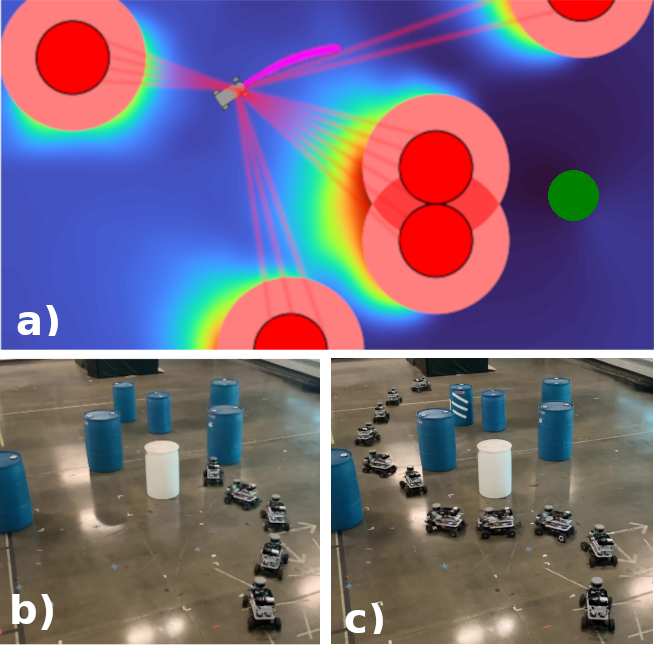
Figure 1: a) Rally car navigating through obstacle field using NMPC with learned value function and lidar. b) Timelapse of rally car navigating through barrels without learned value function (stuck in local minimum). c) Timelapse of rally car navigating through barrels with learned value function (reaches goal).

II Related Work

To enable finite horizon NMPC, many approaches use a global planner to generate receding horizon waypoints to avoid local minima. Sampling-based planners (e.g. RRT and its variants) with simplified or holonomic dynamics are a common choice (e.g. [1, 6]). Alternatively, recent research has investigated the use of learned models to generate waypoints directly from sensor data. A recent autonomous waypoint generation strategy (AWGS) [9] has shown that planning trajectories to waypoints generated by an RL agent can result in shorter trajectories than RRT. Learned waypoints have been used in MPC for drone racing [10], quadrotor navigation in environments with dead-end corridors [11], navigation in real-world cluttered environments [12], and navigation in dynamic environments with other agents [13].

In contrast, our approach aims to circumvent the need to generate local waypoints by augmenting the cost function of the NMPC directly. This is more closely related to Quasi-Infinite Horizon NMPC [14], which uses the solution of an appropriate Lyapunov equation to determine the terminal state cost. This approximates infinite horizon NMPC and has been demonstrated by stabilizing simple ODEs. Quasi-Infinite Horizon NMPC has been built upon to account for active steady-state input constraints [15], waypoint navigation [16], and periodic behaviors [17].

Instead of using the solution to Lyapunov equations to determine the terminal cost, a recent approach suggested the use of a learned approximate value function [18]. This idea was built upon by “Plan Online, Learn Offline” (POLO) [19], which approximates the value function with fitted value iteration and updates the approximate value function online. Deep Value Model Predictive Control [20] extended this by handling stochastic systems explicitly and formulating the running cost as an importance sampler of the value function. MPC-MFRL [21] learned an approximate dynamics model. Model Predictive Q-Learning (MPQ) [22] is closely related to POLO, but also explored the connection between its base NMPC approach, MPPI, and entropy regularized RL. MPQ($\lambda$) [23] built upon this by not only applying the learned value function at the end of the MPC horizon but instead systematically weights it against local Q-function approximations along the trajectories. In this paper, we present an approach which is, to the best of our knowledge, this first to use a learned value function as a terminal cost and constraint in NMPC for perception-based robot navigation and obstacle avoidance.

III Background

Before presenting our approach, we review PAC-NMPC and actor-critic reinforcement learning, which are the foundation of our approach.

III-A PAC-NMPC

Consider the stochastic dynamics given by $p(\mathbf{x}_{t+1}|\mathbf{x}_{t},\mathbf{u}_{t})$ defined by a vector of state values $\mathbf{x}_{t}\in\mathbb{R}^{N_{x}}$, a vector of control inputs $\mathbf{u}_{t}\in\mathbb{R}^{N_{u}}$, and probability density $p$. Probably Approximately Correct NMPC (PAC-NMPC) [7] is a sampling-based SNMPC method which minimizes upper confidence bounds on the expected cost and probability of constraint violation of local feedback policies. It is an Iterative Stochastic Policy Optimization (ISPO) [8], which formulates the search for a control policy $\mathbf{u}_{t}=\bm{\pi}_{t}(\mathbf{x}_{t},\bm{\xi})$ as a stochastic optimization problem, where $\bm{\xi}$ is a set of policy parameters. It does so by iteratively optimizing the hyper-parameters, $\bm{\nu}$, of a surrogate distribution $p(\bm{\xi}|\bm{\nu})$. PAC-NMPC formulates the policy parameters as a nominal control trajectory, $\bm{\xi}~{}=~{}\begin{bmatrix}\bm{\zeta}_{0}^{T}&\bm{\zeta}_{1}^{T}&...&\bm{\zeta}_{N_{T}}^{T}\end{bmatrix}^{T}$, $\bm{\zeta}_{t}\in\mathbb{R}^{N_{u}}$, which is tracked with a feedback policy:

$$\mathbf{u}_{t}=\mathbf{K}_{t}(\bm{\tau}^{d})\left(\mathbf{x}_{t}^{d}-\mathbf{x}_{t}\right)+\mathbf{u}_{t}^{d}(\bm{\xi}).$$ (1)

Here we refer to $\bm{\tau}^{d}\triangleq\{\mathbf{x}_{0}^{d},\mathbf{u}_{0}^{d},\mathbf{x}_{1}^{d},\mathbf{u}_{1}^{d}...,\mathbf{u}_{N_{T}}^{d},\mathbf{x}_{N_{T}+1}^{d}\}$ as the nominal trajectory, which is computed using a nominal deterministic discrete-time dynamics model, $\mathbf{f}(\mathbf{x}_{t}^{d},\mathbf{u}_{t}^{d})$,

$$\mathbf{x}_{t+1}^{d}=\mathbf{x}_{t}^{d}+\mathbf{f}(\mathbf{x}_{t}^{d},\mathbf{u}_{t}^{d})\Delta t$$ (2)

where $\mathbf{u}_{t}^{d}(\bm{\xi})=\bm{\zeta}_{t}$. We use the finite horizon, discrete, time-varying linear quadratic regulator (TVLQR) [24] to compute the feedback gains $\mathbf{K}_{t}(\bm{\tau}^{d})$.

We define a non-negative trajectory cost, $J(\bm{\tau})>0$, and a trajectory constraint $C(\bm{\tau})=\mathbb{I}_{\{g(\bm{\tau})>0\}}$. Here $\bm{\tau}$ represents the discrete time trajectory sequence $\{\mathbf{x}_{0},\mathbf{u}_{0},\mathbf{x}_{1},\mathbf{u}_{1}...,\mathbf{u}_{N_{T}},\mathbf{x}_{N_{T}+1}\}$, where $N_{T}$ is the number of timesteps. Each planning iteration, PAC-NMPC iteratively optimizes

$$\bm{\nu}^{*}=\operatorname*{arg\,min}_{\bm{\nu}}\min_{\alpha>0}(\mathcal{J}^{+}_{\alpha}(\bm{\nu})+\gamma\mathcal{C}^{+}_{\alpha}(\bm{\nu}))$$ (3)

where $\gamma>0$ is a heuristically selected weighting coefficient and

$$\mathbb{P}\left(\mathbb{E}_{\bm{\tau},\bm{\xi}\sim p(\cdot,\cdot|\bm{\nu})}\left[J(\bm{\tau})\right]\leq\mathcal{J}^{+}_{\alpha}(\bm{\nu})\right)\geq 1-\delta$$ (4)

$$\mathbb{P}\left(\mathbb{E}_{\bm{\tau},\bm{\xi}\sim p(\cdot,\cdot|\bm{\nu})}\left[C(\bm{\tau})\right]\leq\mathcal{C}^{+}_{\alpha}(\bm{\nu})\right)\geq 1-\delta$$ (5)

where $1-\delta$ is a heuristically selected confidence bound. These bounds are not only optimization targets, but also provide probabilistic guarantees of performance and safety.

III-B Actor Critic Reinforcement Learning

Consider a Markov decision process (MDP) with states $\mathbf{s}\in\mathbb{R}^{N_{s}}$, actions $\mathbf{a}\in\mathbb{R}^{N_{a}}$, transition dynamics $p(\mathbf{s}_{t+1}|\mathbf{s}_{t},\mathbf{a}_{t})$, and reward function $r(\mathbf{s}_{t},\mathbf{a}_{t})$. The discounted return is defined as the sum of the discounted future rewards of a sequence of states and actions.

$$R^{\gamma}_{t}=\sum_{i=t}^{\infty}\left\{\gamma_{d}^{i-t}r(\mathbf{s}_{i},\mathbf{a}_{i})\right\}$$ (6)

with a discounting factor $\gamma_{d}\in[0,1]$. The action-value function, or Q-function, is the expected discounted return after taking an action $\mathbf{a}_{t}$ from state $\mathbf{s}_{t}$, then following policy $\mathbf{s}_{t}=\pi(\mathbf{a}_{t})$

$$Q^{\pi}(\mathbf{s}_{t},\mathbf{a}_{t})=\mathbb{E}\left[R^{\gamma}_{t}\middle|\mathbf{s}_{t},\mathbf{a}_{t},\pi\right]$$ (7)

The value function is the expected discounted return of following a policy, $\mathbf{s}_{t}=\pi(\mathbf{a}_{t})$, from a given state $\mathbf{s}_{t}$

$$V^{\pi}(\mathbf{s}_{t})=Q^{\pi}(\mathbf{s}_{t},\pi(\mathbf{s}_{t}))=\mathbb{E}\left[R^{\gamma}_{t}\middle|\mathbf{s}_{t},\pi\right]$$ (8)

Actor-critic algorithms learn parameters $\phi$ for an actor policy, $\pi^{\phi}(\mathbf{s})$, and parameters $\psi$ for a critic action-value function, $Q^{\psi}(\mathbf{s},\mathbf{a})$, which estimate the optimal policy $\pi^{*}(\mathbf{s})$ and action-value function $Q^{\pi^{*}}(\mathbf{s},\mathbf{a})$ where

$$\pi^{*}(\mathbf{s}_{t})=\mathbf{a}_{t}^{*}=\operatorname*{arg\,min}_{\mathbf{a}_{t}}\mathbb{E}\left[Q^{\pi^{*}}(\mathbf{s}_{t},\mathbf{a}_{t})\right]$$ (9)

$$Q^{\pi^{*}}(\mathbf{s}_{t},\mathbf{a}_{t}^{*})=\mathbb{E}\left[{r(\mathbf{s}_{t},\mathbf{a}^{*}_{t})+\gamma_{d}Q^{\pi^{*}}(\mathbf{s}_{t+1},\mathbf{a}_{t+1}^{*})}\right]$$ (10)

IV Approach

IV-A Problem Formulation

Our objective is to have a robot navigate through an obstacle field from an initial state $\mathbf{x}_{I}$ to a goal state $\mathbf{x}_{G}$. The robot is equipped with lidar which returns range measurements $\bm{\ell}_{t}=[\ell_{t}^{0}\ \ell_{t}^{1}\ ...\ \ell_{t}^{N_{\bm{\ell}}}]$ at bearings $\bm{\beta}=[\beta^{0}\ \beta^{1}\ ...\ \beta^{N_{\bm{\ell}}}]$ with a maximum range of $\ell_{max}$ at each timestep.

We formulate a generic cost on a finite horizon trajectory,

$$J(\bm{\tau})=\sum_{i=0}^{N_{T}}\left\{q(\mathbf{x}_{i},\mathbf{u}_{i})\right\}+q_{f}(\mathbf{x}_{N_{T}+1})$$ (11)

and impose state bounds and an obstacle constraint.

$$c_{b} =\{\mathbf{x}\ \mid\ \mathbf{x}<\mathbf{x}_{l}\ \text{or}\ \mathbf{x}>\mathbf{x}_{u}\}$$ (12)

$$c_{o} =\{\mathbf{x}\ \mid\ \exists\ \bm{\mathcal{O}}_{j}\ \text{s.t.}\ dist(\mathbf{x},\bm{\mathcal{O}}_{j})\leq r\}$$ (13)

$$c(\mathbf{x}) =\mathbb{I}_{\{c_{b}\cup c_{o}\}}$$ (14)

$$C(\bm{\tau}) =\mathbb{I}_{\{\bigcup_{i=0}^{N_{T}+1}c(\mathbf{x}_{i})\}}$$ (15)

where r is the robot radius, and $\bm{\mathcal{O}}$ are observed obstacle positions. Obstacle positions are calculated as

$$\bm{\mathcal{O}}_{j}=\begin{bmatrix}x_{0}^{x}+cos(x_{0}^{\theta}+\beta^{j})\ell^{j}\\ x_{0}^{y}+sin(x_{0}^{\theta}+\beta^{j})\ell^{j}\\ \end{bmatrix}$$ (16)

for each $\ell^{j}<\ell_{max}$ where $[x_{0}^{x}\ x_{0}^{y}\ x_{0}^{\theta}]^{T}$ is the current position and orientation of the robot.

IV-B Learned Value Function

We formulate an analogous MDP that reflects these costs and constraints:

$$\mathbf{s} =h(\mathbf{x},\bm{\ell})$$ (17)

$$\mathbf{a} =\mathbf{u}$$ (18)

$$r(\mathbf{s},\mathbf{a}) =-q(\mathbf{x},\mathbf{u})-\gamma_{r}c(\mathbf{x})$$ (19)

where $h(\mathbf{x},\bm{\ell})$ maps to the MDP state representation and $\gamma_{r}$ is a heuristically selected constraint violation penalty.

We learn an actor policy, $\pi^{\phi}(\mathbf{s})$, and a critic action-value function, $Q^{\psi}(\mathbf{s},\mathbf{a})$. The value function is then reconstructed as

$$V^{\psi\phi}(\mathbf{x},\bm{\ell})=Q^{\psi}(\mathbf{s},\pi^{\phi}(\mathbf{s}))$$ (20)

In this paper, we learn the actor and critic using Twin Delayed Deep Deterministic Policy Gradients (TD3) [25], a state-of-the-art actor-critic method. However, our approach is agnostic the method used to approximate the value function.

IV-C PAC-NMPC with Learned Value Function

In order to use the learned value function as a terminal state cost, we must form an estimate of the future lidar measurement, $\widehat{\bm{\ell}}_{N_{T}+1}$, at the terminal state of a sampled trajectory based on the current lidar measurement, $\bm{\ell}_{0}$. First, we calculate observed obstacle positions, $\bm{\mathcal{O}}$, from the current state and lidar measurement (eq. 16). Then, we calculate the range, $\widehat{l}^{j}$, and bearing, $\widehat{\beta}^{j}$, to each observed obstacle from the terminal state:

$$\widehat{l}^{j} =\sqrt{(x_{N_{t}+1}^{x}-\mathcal{O}_{j}^{x})^{2}+(x_{N_{t}+1}^{y}-\mathcal{O}_{j}^{y})^{2}}$$ (21)

$$\widehat{\beta}^{j} =\operatorname{atan2}(x_{N_{t}+1}^{y}-\mathcal{O}_{j}^{y},x_{N_{t}+1}^{x}-\mathcal{O}_{j}^{x})-x_{N_{T}+1}^{\theta}$$ (22)

where $[x_{N_{t}+1}^{x}\ x_{N_{t}+1}^{y}\ x_{N_{t}+1}^{\theta}]^{T}$ is the position and orientation of the robot at the terminal state of the trajectory. We set the lidar estimates as

$$\widehat{\ell}_{N_{T}+1}^{k} =\widehat{\ell}^{j}$$ (23)

$$k =\operatorname*{arg\,min}_{k}\{abs(\widehat{\beta}^{j}-\beta_{k})\}$$ (24)

We can then set the terminal cost as the negative learned value function (i.e, the approximate cost-to-go).

$$q_{f}(\mathbf{x}_{N_{T}+1})=-V^{\psi\phi}(\mathbf{x}_{N_{T}+1},\widehat{\bm{\ell}}_{N_{T}+1})$$ (25)

This approximates the infinite horizon trajectory cost given the current lidar measurement.

$$J(\bm{\tau}) =\sum_{i=0}^{N_{T}}\left\{q(\mathbf{x}_{i},\mathbf{u}_{i})\right\}-V^{\psi\phi}(\mathbf{x}_{N_{T}+1},\widehat{\bm{\ell}}_{N_{T}+1})$$ (26)

$$\approx\sum_{i=0}^{N_{T}}\left\{q(\mathbf{x}_{i},\mathbf{u}_{i})\right\}+\mathbb{E}\left[\sum_{i=N_{T}+1}^{\infty}\left\{\gamma q(\mathbf{x}_{i},\mathbf{u}_{i})\right\}\;\middle|\;\bm{\ell}_{0}\right]$$

We also enforce an additional constraint: that the learned value function improves from the current state to the final state of the trajectory.

$$C_{V} =\{\bm{\tau}\ \mid\ V(\mathbf{x}_{N_{T}+1},\widehat{\bm{\ell}}_{N_{T}+1})>V(\mathbf{x}_{0},\bm{\ell})\}$$ (27)

$$C(\bm{\tau}) =\mathbb{I}_{\{\bigcup_{i=0}^{N_{T}+1}c(\mathbf{x}_{i})\cup C_{V}\}}$$ (28)

Each planning interval, PAC-NMPC optimizes and returns policy hyperparameters, $\bm{\nu}^{*}$, a PAC bound on the expected cost, $\mathcal{J}^{+}_{\alpha}(\bm{\nu}^{*})$, and a PAC bound on the probability of constraint violation, $\mathcal{C}^{+}_{\alpha}(\bm{\nu}^{*})$. These bounds serve as performance and safety guarantees. In this context, if the robot executes a policy with parameters sampled from the optimized surrogate distribution, $p(\bm{\xi}|\bm{\nu}^{*})$, then the probability of violating the obstacle constraint or worsening the learned value function, given the current lidar measurement, will be less than $\mathcal{C}^{+}_{\alpha}(\bm{\nu})$ with a probability of $1-\delta$ (eq. 5).

V Simulation Experiments

V-A Dynamics, Costs, and Constraints

We simulate a stochastic bicycle model with acceleration and steering rate inputs. We denote ${\mathbf{x}_{t}}=[x_{0},x_{1},x_{2},x_{3},x_{4}]^{T}$ as the state vector, ${\mathbf{u}_{t}}=[u_{0},u_{1}]^{T}$ as the control vector, $l=0.33$ as the wheelbase, and $\bm{\Gamma}=diag(\left[0.0004,0.0004,0.0116,0.1004,0.0056\right])$ as the covariance, which was fit from hardware data (as described in Section VI).

$$\mathbf{x}_{t+1} \sim p(\cdot|\mathbf{x}_{t},\mathbf{u}_{t})\triangleq\mathbf{x}_{t}+\left(f(\mathbf{x}_{t},\mathbf{u}_{t})+\bm{\omega}\right)\Delta t$$

$$f(\mathbf{x}_{t},\mathbf{u}_{t}) =[x_{3}\cos(x_{2}),x_{3}\sin(x_{2}),x_{3}\tan(x_{4})/l,u_{0},u_{1}]$$

$$\bm{\omega} \sim\mathcal{N}(\cdot|\mathbf{0},\bm{\Gamma})$$ (29)

The acceleration is constrained to $(-1.0,1.0)\frac{m}{s}$, the steering rate to $(-1.0,1.0)\frac{rad}{s}$, and the steering angle to $(-0.4,0.4)$ rad.

We use a quadratic state cost

$$q(\mathbf{x},\mathbf{u})=(\mathbf{x}-\mathbf{x}_{G})^{T}Q(\mathbf{x}-\mathbf{x}_{G})$$ (30)

where $Q=diag([0.01\ 0.01\ 0.00\ 0.00\ 0.00])$. We also apply a velocity constraint such that $v_{min}\leq x_{3}\leq v_{max}$ where $v_{min}=-1.0\frac{m}{s}$ and $v_{max}=3.0\frac{m}{s}$.

When running PAC-NMPC, we optimize a 12 timestep trajectory with $\Delta t=0.1$ sec at a replanning period of $H=0.2$ sec, and we interpolate the feedback policies to 50Hz. We set PAC-NMPC parameters as $L=5$, $M=1024$, $\delta=0.05$, $\gamma=2$ and normalize the sampled trajectory costs before optimizing the PAC bounds to achieve tighter bounds.

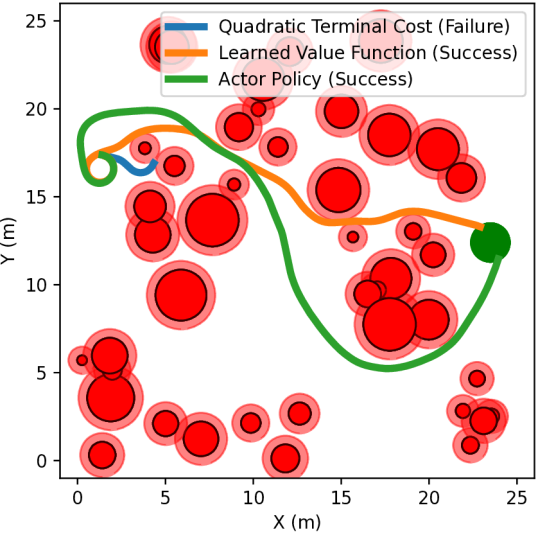
Figure 2: Testing environment where PAC-NMPC fails without the learned value function as the terminal cost and constraint. The goal region is shown in green, obstacles in solid red, and the obstacle constraint region in translucent red.

V-B Actor Critic Training

We trained the actor and critic in simulation with the stochastic bicycle model and a 64 beam $360^{\circ}$ lidar with a minimum range of $\ell_{min}=0.1$ meters and maximum range of $\ell_{max}=10$ meters. Non-detections in the lidar measurement were set to the maximum range.

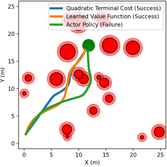
Figure 3: Testing environment where the actor policy violates the obstacle constraint.

Randomly sampled training environments consisted of an initial state, $\mathbf{x}_{I}$, a goal state $\mathbf{x}_{G}$, and obstacles. $\mathbf{x}_{I}$ and $\mathbf{x}_{G}$ were uniformly sampled between $\mathbf{x}_{min}=[0\ 0\ -\pi\ 0\ -0.4]^{T}$ and $\mathbf{x}_{max}=[25\ 25\ -\pi\ 0\ 0.4]^{T}$. The number of obstacles was uniformly sampled between $0$ and $50$, the radius of each obstacle was uniformly sampled between $0.25$ and $1.5$ meters, and the obstacle positions were randomly sampled between $\mathbf{p}_{min}=[0\ 0]^{T}$ and $\mathbf{p}_{max}=[25\ 25]^{T}$. If $\mathbf{x}_{I}$ or $\mathbf{x}_{G}$ were in collision with an obstacle, the environment was discarded. When a training episode reached 250 steps, the system violated a constraint, or the system reached the goal, the episode ended and a new environment was sampled.

The MDP state, $\mathbf{s}$, consisted of the velocity, the tangent of the steering angle, the range to the goal, cosine and sine of the bearing to the goal, and the lidar measurement.

$$s =h(\mathbf{x},\bm{\ell})=\begin{bmatrix}\dfrac{x_{3}-v_{min}}{v_{max}-v_{min}}\\ \dfrac{\tan(x_{4})-\tan(-0.4)}{\tan(0.4)-\tan(-0.4)}\\ \dfrac{{\|{[d_{0}\ d_{1}]^{T}}\|}}{{\|{\mathbf{p}_{max}-\mathbf{p}_{min}}\|}}\\ \cos(\beta_{G}-x_{2})\\ \sin(\beta_{G}-x_{2})\\ \dfrac{\bm{\ell}-\ell_{min}}{\ell_{max}-\ell_{min}}\end{bmatrix}$$ (31)

$$\mathbf{d} =[d_{0}\ d_{1}\ d_{2}\ d_{3}\ d_{4}]^{T}=\mathbf{x}_{G}-\mathbf{x}$$ (32)

$$\beta_{G} =\operatorname{atan2}(d_{1},d_{0})$$ (33)

This MDP state normalizes the NMPC state, includes the lidar measurement, and precomputes several trigonometric functions.

We use shallow, fully connected neural networks as the function approximators for $\pi^{\phi}(\mathbf{s})$ and $Q^{\psi}(\mathbf{s},\mathbf{a})$. Each neural network has two hidden layers with 256 nodes, ReLU activation functions, and 10% dropout after each hidden layer. When using the learned value function for the terminal cost and constraint, we sample dropout masks to incorporate network uncertainty into the PAC bound computation. We train the networks until the mean actor loss, evaluated over 100 training steps, stops improving. For this experiment, it trained in around 1.8 million steps, which took 1.9 hours.

V-C Experimental Results

We generated 100 random environments from the training distribution. In order to provide meaningful testing environments, environments in which no obstacles blocked the path to the goal were discarded. We also set the initial state of the robot to always point towards the goal. Simulations were run on a laptop with an Intel Core i-9-13900H CPU and a Nvidia GeForce RTX 4080 Max-Q GPU.

We compared performance when using two different terminal costs. First, we tested a quadratic final cost, $q_{f}(\mathbf{x}_{N_{T}+1})=(\mathbf{x}-\mathbf{x}_{G})^{T}Q_{f}(\mathbf{x}-\mathbf{x}_{G})$ where $Q_{f}=diag([1\ 1\ 0\ 0\ 0])$. Then, we tested with the learned value function, $q_{f}(\mathbf{x}_{N_{T}+1})=-V^{\psi\phi}(\mathbf{x}_{N_{T}+1},\widehat{\bm{\ell}}_{N_{T}+1})$, and the value function improvement constraint (eq. 28). We found that when using the quadratic terminal cost, the system was only able to reach the goal in 76% of trials, often getting caught in local minima. When using the learned value function, the system was able to reach the goal in 97% of trials (Fig. 2, 5).

Since our method for learning the value function generates an actor policy, we also compared our approach against this policy directly. The actor policy only reached the goal without violating constraints in 90% of trials. Since it was unable to explicitly enforce constraints, it violated the obstacle constraint in 6% of trials and violated the velocity constraint in 1% of trials (Fig. 3, 5). This highlights an advantage of using NMPC when operating in safety critical environments.

In Figure 4, we plot the optimized PAC bounds at each planning interval for the “learned value function” trial in Figure 3. To validate PAC bounds, we compare them against Monte Carlo estimates of the expected cost and probability of constraint violation. On average, PAC-NMPC produced guarantees that the probability of constraint violation of the NMPC generated policies would be less than 5%. These bounds verify that the policies will, with a high probability, not violate the collision constraint and produce feedback policies that will reduce the approximate cost-to-go, given the current perception information.

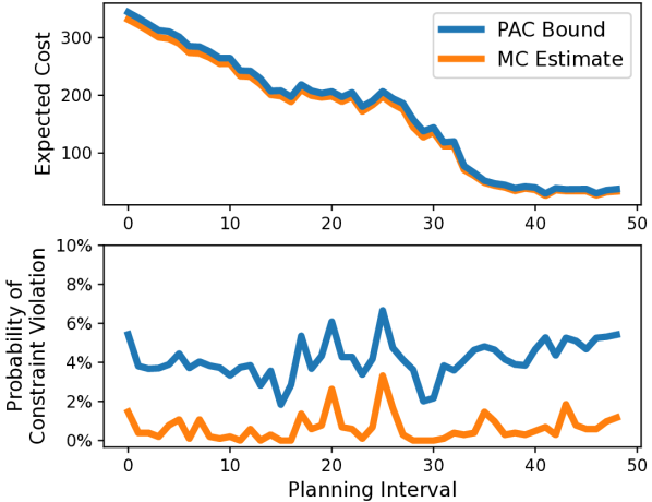
Figure 4: Optimized PAC Bounds compared to Monte Carlo estimates at each planning interval for the “learned value function” trial in Figure 3.

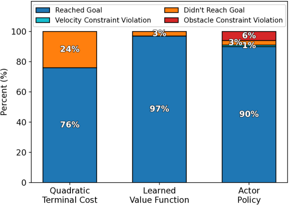
Figure 5: Percentage of trials in which the system reached the goal, didn’t reach the goal, and violated constraints.

VI Hardware Experiments

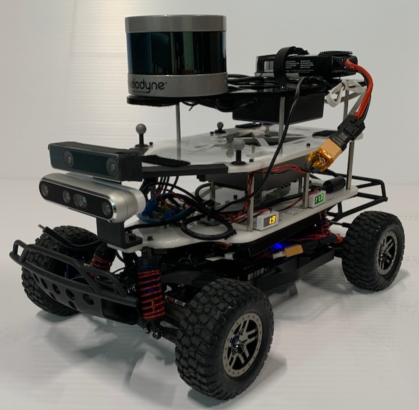
Figure 6: 1/10^th scale Traxxas Rally Car platform with a Nvidia Jetson Orin, variable electronic speed controller, and Velodyne Puck LITE lidar.

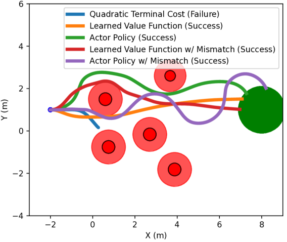
Figure 7: Testing environment where PAC-NMPC fails without the learned value function as the terminal cost

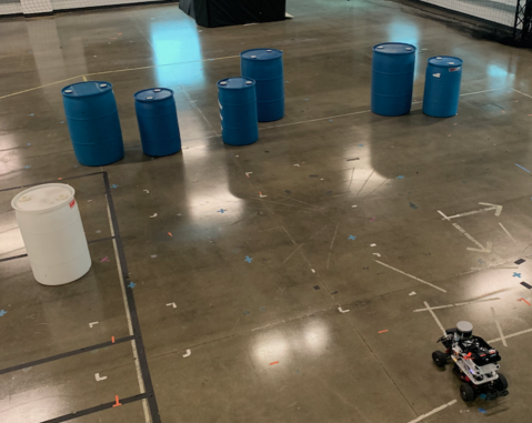
Figure 8: Example hardware environment setup

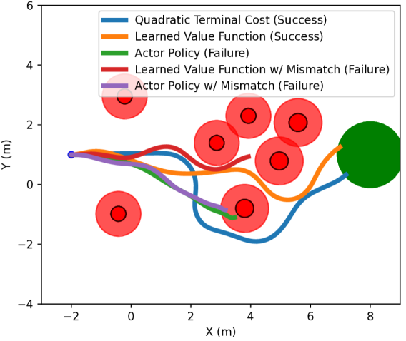
Figure 9: Testing environment where the agent network causes a collision.

VI-A Hardware

To evaluate our approach on physical hardware, we used a 1/10^th scale Traxxas Rally Car platform (Fig. 6). The algorithm runs on a Nvidia Jetson Orin mounted on the bottom platform. The control interface is a variable electronic speed controller (VESC), which executes commands and provides servo state information. A Velodyne Puck LITE lidar is mounted on the top platform. The position and orientation were tracked with an OptiTrack motion capture system.

We model the rally car dynamics as a stochastic bicycle model where noise is modeled as a Gaussian distribution with $\bm{\Gamma}=diag(\left[0.001,0.001,0.014,0.079,0.006\right])$ as the covariance (eq. 29). The distribution was fit from 6448 samples of data collected with the car in the motion capture system. For hardware experiments, we used the same value function that was trained entirely in simulation. We also train a value function with an incorrect wheelbase, $L=0.5$, to demonstrate the utility of our approach even in the presence of model mismatch. When using the value function on hardware, we downsampled the Velodyne Puck lidar measurements to $N_{\bm{\ell}}=64$ to match the simulated sensor.

We generated 20 random environments consisting of a maximum of 8 circular obstacles in an 8 meter by 6 meter space. We discarded environments in which obstacles overlapped or in which no obstacles were blocking the path to the goal. We placed barrels at these random positions in the motion capture system (Fig. 8).

VI-B Results

We compared performance when using the quadratic terminal cost, $q_{f}(\mathbf{x}_{N_{T}+1})=(\mathbf{x}-\mathbf{x}_{G})^{T}Q_{f}(\mathbf{x}-\mathbf{x}_{G})$ where $Q_{f}=diag([1\ 1\ 0\ 0\ 0])$, and the learned value function, $q_{f}(\mathbf{x}_{N_{T}+1})=-V(\mathbf{x}_{N_{T}+1},\widehat{\bm{\ell}}_{N_{T}+1})$, with the value function improvement constraint (eq. 28). We found that when using the quadratic terminal cost, the system was only able to reach the goal in 65% of trials, often getting caught in local minima. When using the learned value function, the system was able to reach the goal in 95% of trials (Fig. 7, 10). We also compared our approach directly against the actor policy, which was only able to reach the goal without colliding in 85% of trials (Fig. 9, 10).

When using the learned value function trained with the incorrect wheelbase, but using the correct wheelbase for sampling NMPC trajectories, the system was able to reach the goal in 80% of trials, which is still an improvement over the quadratic terminal cost. On the other hand, the agent policy trained with the incorrect wheelbase collided in 30% of trials. Thus, although using an RL actor trained in the presence of model mismatch could be dangerous in safety critical environments, our approach can still safely benefit from such RL trained models.

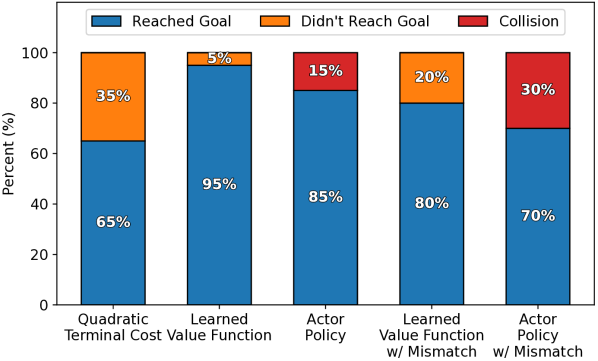
Figure 10: Percentage of trials in which the system reached the goal, didn’t reach the goal, and collided.

VII Discussion

In this paper, we presented an SNMPC approach utilizing a learned perception informed value function capable of navigating through an obstacle field using lidar. We demonstrated, both in simulation and on hardware, that using the learned value function as a terminal cost and constraint enabled the controller to avoid local minima without violating obstacle constraints. Further, we showed that our approach was able to generate statistical guarantees of performance and safety in real time, which may improve confidence in the controllers ability to use learned components in safety critical environments. Future work could explore the quantification of perception uncertainty itself as well as updating the learned value function online.

References

- [1] A. Polevoy, M. Basescu, L. Scheuer, and J. Moore, “Post-stall navigation with fixed-wing uavs using onboard vision,” in 2022 International Conference on Robotics and Automation (ICRA). IEEE, 2022, pp. 9696–9702.
- [2] A. Polevoy, C. Knuth, K. M. Popek, and K. D. Katyal, “Complex terrain navigation via model error prediction,” in 2022 International Conference on Robotics and Automation (ICRA). IEEE, 2022, pp. 9411–9417.
- [3] D. Falanga, P. Foehn, P. Lu, and D. Scaramuzza, “Pampc: Perception-aware model predictive control for quadrotors,” in 2018 IEEE/RSJ International Conference on Intelligent Robots and Systems (IROS). IEEE, 2018, pp. 1–8.
- [4] K. Lee, J. Gibson, and E. A. Theodorou, “Aggressive perception-aware navigation using deep optical flow dynamics and pixelmpc,” IEEE Robotics and Automation Letters, vol. 5, no. 2, pp. 1207–1214, 2020.
- [5] B. Brito, B. Floor, L. Ferranti, and J. Alonso-Mora, “Model predictive contouring control for collision avoidance in unstructured dynamic environments,” IEEE Robotics and Automation Letters, vol. 4, no. 4, pp. 4459–4466, 2019.
- [6] Z. Jian, Z. Yan, X. Lei, Z. Lu, B. Lan, X. Wang, and B. Liang, “Dynamic control barrier function-based model predictive control to safety-critical obstacle-avoidance of mobile robot,” in 2023 IEEE International Conference on Robotics and Automation (ICRA). IEEE, 2023, pp. 3679–3685.
- [7] A. Polevoy, M. Kobilarov, and J. Moore, “Probably approximately correct nonlinear model predictive control (pac-nmpc),” IEEE Robotics and Automation Letters, pp. 1–8, 2023.
- [8] M. Kobilarov, “Sample complexity bounds for iterative stochastic policy optimization,” Advances in Neural Information Processing Systems, vol. 28, 2015.
- [9] S. Sharma and M. E. Taylor, “Autonomous waypoint generation strategy for on-line navigation in unknown environments,” environment, vol. 2, p. 3D, 2012.
- [10] E. Kaufmann, A. Loquercio, R. Ranftl, A. Dosovitskiy, V. Koltun, and D. Scaramuzza, “Deep drone racing: Learning agile flight in dynamic environments,” in Conference on Robot Learning. PMLR, 2018, pp. 133–145.
- [11] C. Greatwood and A. G. Richards, “Reinforcement learning and model predictive control for robust embedded quadrotor guidance and control,” Autonomous Robots, vol. 43, pp. 1681–1693, 2019.
- [12] S. Bansal, V. Tolani, S. Gupta, J. Malik, and C. Tomlin, “Combining optimal control and learning for visual navigation in novel environments,” in Conference on Robot Learning. PMLR, 2020, pp. 420–429.
- [13] B. Brito, M. Everett, J. P. How, and J. Alonso-Mora, “Where to go next: Learning a subgoal recommendation policy for navigation in dynamic environments,” IEEE Robotics and Automation Letters, vol. 6, no. 3, pp. 4616–4623, 2021.
- [14] H. Chen and F. Allgöwer, “A quasi-infinite horizon nonlinear model predictive control scheme with guaranteed stability,” Automatica, vol. 34, no. 10, pp. 1205–1217, 1998.
- [15] G. Pannocchia, S. J. Wright, and J. B. Rawlings, “Existence and computation of infinite horizon model predictive control with active steady-state input constraints,” IEEE Transactions on Automatic Control, vol. 48, no. 6, pp. 1002–1006, 2003.
- [16] F. de Almeida, “Waypoint navigation using constrained infinite horizon model predictive control,” in AIAA Guidance, Navigation and Control Conference and Exhibit, 2008, p. 6462.
- [17] T. Erez, Y. Tassa, and E. Todorov, “Infinite-horizon model predictive control for periodic tasks with contacts,” Robotics: Science and systems VII, p. 73, 2012.
- [18] M. Zhong, M. Johnson, Y. Tassa, T. Erez, and E. Todorov, “Value function approximation and model predictive control,” in 2013 IEEE symposium on adaptive dynamic programming and reinforcement learning (ADPRL). IEEE, 2013, pp. 100–107.
- [19] K. Lowrey, A. Rajeswaran, S. Kakade, E. Todorov, and I. Mordatch, “Plan online, learn offline: Efficient learning and exploration via model-based control,” arXiv preprint arXiv:1811.01848, 2018.
- [20] D. Hoeller, F. Farshidian, and M. Hutter, “Deep value model predictive control,” in Conference on Robot Learning. PMLR, 2020, pp. 990–1004.
- [21] Z.-W. Hong, J. Pajarinen, and J. Peters, “Model-based lookahead reinforcement learning,” arXiv preprint arXiv:1908.06012, 2019.
- [22] M. Bhardwaj, A. Handa, D. Fox, and B. Boots, “Information theoretic model predictive q-learning,” in Learning for Dynamics and Control. PMLR, 2020, pp. 840–850.
- [23] M. Bhardwaj, S. Choudhury, and B. Boots, “Blending mpc & value function approximation for efficient reinforcement learning,” arXiv preprint arXiv:2012.05909, 2020.
- [24] R. Tedrake, Underactuated Robotics, 2022. [Online]. Available: http://underactuated.mit.edu
- [25] S. Fujimoto, H. Hoof, and D. Meger, “Addressing function approximation error in actor-critic methods,” in International conference on machine learning. PMLR, 2018, pp. 1587–1596.