Investigating Efficient Deep Learning Architectures For Side-Channel Attacks on AES

Abstract

Over the past few years, deep learning has been getting progressively more popular for the exploitation of side-channel vulnerabilities in embedded cryptographic applications, as it offers advantages in terms of the amount of attack traces required for effective key recovery. A number of effective attacks using neural networks have already been published, but reducing their cost in terms of the amount of computing resources and data required is an ever-present goal, which we pursue in this work.

This project focuses on the ANSSI Side-Channel Attack Database (ASCAD). We produce a JAX-based framework for deep-learning-based SCA, with which we reproduce a selection of previous results and build upon them in an attempt to improve their performance. We also investigate the effectiveness of various Transformer-based models.

Keywords Deep Learning  $\cdot$ Cryptography  $\cdot$ Side-Channel Attacks  $\cdot$ Profiling Attacks

1 Introduction

1.1 Context: Side-Channel Attacks

Side-Channel Attacks (or SCA) are a class of cyberattacks that exploit weaknesses specific to implementions of would-be secure systems. For information recovery, they may rely on correlation between the targeted data and variations in timing [Koc96], power consumption and electromagnetic (EM) emissions [RD20], sound emission [GST17], and other characteristics of a system. They may rely on the system’s failure behavior, through Differential Fault Analysis [DLV03]. If a suitable side-channel vulnerability exists in its implementation(s), even a fully theoretically-secure algorithm can be cracked.

The implementer of a system may try to minimize information leakage through countermeasures. These may include performing sensitive operations in constant time; always executing the same code regardless of the input fed to the system; avoiding the direct manipulation of sensitive data through masking; etc. They may also include physical defense mechanisms, such as EM shielding.

Side-channel attacks may be profiling or non-profiling, the difference being that the attacker has access to a copy of the target device in the profiling case. In this work, we will focus on profiling attacks, into which machine learning techniques have been making headway. In particular, neural networks have been studied due to their ability to recover information even from highly-protected implementations.

As new attacks are published, increasingly-effective countermeasures are developed, rendering further attacks more costly both in terms of computing power required to train the models, and in terms of the amount of data that must be collected in order to apply them. As such, enhancing the information-recovery capabilities of neural networks used for SCA is of major interest.

So far, in practice, even neural networks are typically unable to reliably recover the correct value of a given key byte from a single trace. As such, guesses made over multiple traces are combined to obtain a more reliable one. The minimum number of traces required for reliable recovery of the target variable is commonly referred to as "guessing entropy" in the literature.

In this project, we focus on power consumption and EM traces. We use the ASCAD project, described below, as a source of data and as a starting point.

1.2 Overview of ASCAD

ASCAD (ANSSI SCA Database) [AC21] is a collection of power trace databases for side-channel attacks. Since the introduction of its first version, has enjoyed significant popularity in the SCA community as a benchmark for deep-learning-based attacks.

Thus far, it comprises two main versions, both targeting AES and collected on different microcontrollers and AES implementations. The project comes with a set of pre-trained models targeting each database, as well as code to train them.

Each set of databases is provided with "raw" traces, covering some portion of the encryption/decryption process, and "extracted" traces, covering a subset of the former which is known to leak relevant information. Extracted traces come with precomputed labels, corresponding to intermediate variables manipulated during the encryption/decryption process from which the key can be recovered. It is significantly easier to recover a well-chosen intermediate variable then post-process it to compute the key than to try to recover the key directly.

Traces may be synchronized or desynchronized. In the synchronized case, a given timestep always corresponds to the same instant in the encryption or decryption process, whereas such an instant may be represented at different time steps in the desynchronized case. Desynchronization implies the need for some degree of shift invariance or equivariance in the network’s feature extraction process.

1.2.1 ASCADv1 - Implementation on ATMega8515

Described in [Ben+20], ASCADv1 has two campaigns (themselves ambiguously named v1 and v2 - we refer to them as "fixed key" and "variable key") targeting a software AES implementation on ATMega8515 [Ben+18], which uses boolean masking.

The fixed-key campaign uses the same key for profiling and attack sets, whereas the variable-key campaign uses a random key for profiling and a fixed one for attack.

They are structured as shown in Table 1.

Table 1: ASCADv1 (ATMega) datasets (SPET/SPRT = Samples Per Extracted/Raw Trace)

Version	N° Profiling traces	N° Attack traces	SPET	SPRT
v1 / fixed key	50,000	10,000	700	100,000
v2 / variable key	200,000	100,000	1400	250,000

The README file for the variable-key campaign mentions that the traces are "not synchronized". The traces do appear synchronized to some degree; the magnitude of the desynchronization is not explicited.

Additionally, the variable key dataset exhibits significant qualitative differences from the fixed key dataset, as one can see on Figure 1.

Figure 1: Comparison of traces between ASCAD fixed-key and variable-key ATMega datasets

These differences were not clearly documented: no mention of the variable-key dataset was made in [Ben+20], and no explanation was provided in the repository.

They were noticed by other researchers, but clarification thus far has been incomplete [Com] regarding the precise method of measurement for each campaign. Nevertheless, the difference in goals behind each campaign is to be noted:

"The fixed key campaign was measured with a strong incentive to get a clean signal in order to make sure that simple attacks could be performed, while this effort was not stressed in the random key campaign, which aims at being more challenging. This explains the notable difference of sampling rate and signal quality that you observed." - @rb-anssi (Ryad Benadjila)

The lack of clarity around the nature of the datasets, along with the relative scarcity of papers exploiting the variable-key one, represented a significant source of confusion at the beginning of this project. It was originally incorrectly assumed that published attacks focused on the variable-key dataset, as the performance of a network on the fixed-key dataset said little about its ability to generalize to different keys.

1.2.2 ASCADv2 - Implementation on STM32F303RCT7

Described in [MS21], ASCADv2 has a single campaign, with a total of 800,000 traces. The "extracted" dataset features a profiling set of 500,000 traces using random keys, and an attack set of 10,000 traces using random keys as well. The paper claims 700,000 profiling traces, 20,000 validation traces and 50,000 test traces, but the data linked on the project’s GitHub appears to be different from the one it describes.

The AES implementation it targets [RT19] uses affine masking [Fum+10] as a side-channel countermeasure instead of the simpler boolean masking technique used on the ATMega8515.

Except for data exploration, our tests were not applied to ASCADv2 over the course of this project. We had initially hoped to do so, but ASCADv1 by itself presented difficulties that we wanted to resolve first.

1.3 Prior work on ASCAD

Ever since ASCAD’s introduction, there has been a notable body of research on efficient architectures for attacks on the database, in addition to the ones put forth in the original paper. We chose to focus on a handful of them, described below.

1.3.1 Original ASCADv1 networks

[Ben+20] explored Multi-Layer Perceptrons (MLPs), and several Convolutional Neural Network (CNN) architectures: VGG-16 [SZ15], ResNet-50 [He+15] and Inception-v3 [Sze+15].

CNNs and MLPs had comparable performance in the synchronized key, but CNNs vastly outperformed MLPs in the presence of the desynchronization, owing to the translation equivariance of convolutions. Among CNNs, a VGG-16-inspired network had the best accuracy.

Training setup:

• Optimizer: RMSProp

• Learning rate schedule: constant at $10^{-5}$

• Preprocessing: none (unscaled, uncentered traces)

1.3.2 "Methodology for Efficient CNN Architectures in Profiling Attacks"

[Zai+19] put forth a disciplined methodology to build efficient CNNs for profiling attacks. It uses relatively shallow architectures, with short filters, leverages batch normalization [IS15] and a one-cycle learning rate schedule.

In parallel, the authors used gradient [MDP19] and activation visualization to pinpoint the timesteps considered to be of interest by the network, and compared them to Signal-to-Noise Ratio (SNR) analyses on intermediate variables of interest.

For ASCADv1, its best network in the synchronized case has 3,930 times fewer parameters than the previous state of the art, and has a greater information recovery capability, requiring 191 traces for a zero-entropy key recovery, against a previous best of 1,146. Only the fixed-key dataset was investigated by the authors.

Training setup:

• Optimizer: Adam [KB17]

• Learning rate schedule: linear one-cycle with maximum of $10^{-3}$

• Preprocessing: point-wise (synchronized) / none (desynchronized)

1.3.3 "Pay Attention to Raw Traces: A Deep Learning Architecture for End-to-End Profiling Attacks"

The approach proposed in [Lu+21] (P.A.R.T.) sets itself apart from others by being able to take "raw" traces as input - that is, traces covering a significant part of the encryption/decryption cycle, and not just a small window in which there is high information leakage. In that respect, it does away with the need for the selection of Points Of Interest (POIs) prior to network training and evaluation.

In order to be able to achieve that goal without running into the so-called "curse of dimensionality" and the accompanying explosion in resource consumption, P.A.R.T. first employs a so-called "junior encoder", which encodes overlapping time windows with a width of 1-2 clock cycles into a much shorter sequence:

Synchronized setting

Two sequences of time windows are encoded by locally-connected layers with stride equal to their width, a single filter and an offset of half their width between them. They are then concatenated. This significantly reduces the dimensionality of the output fed to subsequent layers.

Desynchronized setting

A stride of 1 is used for the first layer, which leads to no dimensionality reduction besides that ensuing from the lack of padding. This reduction is achieved by stacking convolutional layers with kernels of length 3 and a stride of 1 still, and max-pooling layers. The final number of channels is 128. Data augmentation is applied by randomly shifting the input in addition to its original desynchronization.

After the junior encoder, a "senior encoder" is used to combine features across time, using bidirectional LSTMs. It is followed by a simple multiplicative attention mechanism and a feed-forward classifier.

Once fully converged, the authors’ networks can recover a key from both datasets in under 10 traces.

N.B.: In this paper, the ASCADv1 (ATMega) fixed-key dataset is described as "ASCAD v1", and the variable-key dataset as "ASCAD v2".

1.3.4 Original ASCADv2 network

The neural network proposed in [MS21] is a derivative of ResNet [He+15]. It uses multi-task learning to recover information about the masking parameters and about each key byte simultaneously, with a common trunk for feature extraction followed by branches specific to each predicted variable.

1.4 Transformer and derivatives

The introduction of the Transformer architecture in [Vas+17], whose fundamental characteristic is the pervasive use of attention, represented a major leap forward in deep learning. Since then, its derivatives have been successfully applied to Natural Language Processing (NLP) [Dev+19, Rad+19, Bro+20], Computer Vision [Dos+21, Wu+21], speech recognition [Sah+22, GCG21], symbolic computation [LC19], etc., regularly producing new state-of-the-art results. The vast flexibility of this family of architectures made it a natural candidature for evaluation in the SCA context, which, to our knowledge, had not been done before.

Transformer models take a (potentially variable-length) sequence of tokens as input, and return a sequence with the same shape. To perform classification, this sequence may then be aggregated into a single token, for example through global average pooling, or through extraction of the embedding corresponding to a special, learned token, such as BERT’s [CLS] [Dev+19].

Below, we detail some of the considerations specific to Transformers.

1.5 Positional encoding

By itself, the attention mechanism cannot distinguish between positions in the input sequence. As such, additional features, called positional encoding, are typically added or concatenated to the input embeddings before they are fed to a Transformer trunk. They may be learnable, or deterministic, for example using Fourier features as in the original Transformer paper.

A significant number of such features may be required for the model to accurately leverage positional information; it is typically on the order of a few hundreds. This represents a significant overhead if the input tokens have low dimensionality.

Some models, such as CvT [Wu+21] or Audiomer [Sah+22], do away with positional encodings altogether by leveraging the spatially-aware inductive bias of convolutions, applying them to tokens repeatedly within the Transformer trunk.

1.5.1 Training setup

A major drawback of Transformer models thus far has been their high cost of training. Though they do not necessarily have more trainable parameters than comparable alternatives, the most popular Transformers do, and were designed with very-large-scale training setups in mind. Derivative works rely on fine-tuning more often than not, due to the unfeasibility of training those models from scratch on a modestly-sized infrastructure.

One reason for this high cost is the amount of data required by Transformers to generalize well, which is typically extremely large: BERT [Dev+19] was pretrained on 3.3 billion words, and GPT-3 [Bro+20] on nearly 500 billion tokens; ViT [Dos+21] performs much worse than ResNet when pretrained on a dataset of 9 million images, but better when over 90 million images are used. This may be explained by the flexibility of the attention mechanism, which is both a strength and a weakness, as it lacks the inductive bias that led CNNs to revolutionize computer vision in the early 2010s.

To train Transformers in the face of a small dataset, data augmentation is nearly a requirement. While various modalities of data augmentation have been extensively studied and implemented in the vision and audio subfields of machine learning, they may be delicate to implement in the SCA context - beyond simple desynchronization - without destroying the relevant information carried by traces.

Additionally, Transformers are trained with adaptive optimizers such as Adam [KB17], LARS [YGG17] or LAMB [You+20]. Use of a learning rate schedule including warm-up is a necessity to ensure stability, and proper hyperparameter tuning is recommended. Detailed training guidelines may be found in [PB18].

1.5.2 Taming quadratic complexity

Another reason for Transformers’ high training cost is the $O(n^{2})$ time and space complexity of the self-attention mechanism with respect to the length of the input sequence, which typically renders it impractical for sequences longer than a few hundred or a few (low single digits) thousand entries.

A variety of methods exist to work around the latter problem; we describe them below.

Artificial reduction of the sequence length

This is the standard, most common workaround. For signal processing, this may be done by splitting the input into potentially-overlapping patches of a set size [Dos+21], often with additional preprocessing such as Short-Time Fourier Transforms (STFTs) [GCG21, Ell+21].

Performing self-attention on a fixed-size latent array

Perceiver [Jae+21a] and Perceiver IO [Jae+21] by DeepMind use a novel architecture, wherein the model’s trunk transforms a latent array whose initial value is learned, and whose size is independent of the input sequence. Cross-attention is performed between the input and the latent array several times across a forward pass, but less often than self-attention on the latent array. The resulting model has $O(m(m+n))$ complexity, where $m$ is the length of the latent array and $n$ the length of the input. This architecture is particularly relevant for multi-modality processing (video, audio, sound) with a single model, as modalities can be distinguished using their additional dimensions in the embeddings of the corresponding data.

Reducing the complexity of the attention mechanism itself

This approach has notably been proposed in the Reformer [KKL20] and Performer [Cho+21] papers. Reformers use a memory-efficient training process by computing attention scores separately for each query, to avoid storing a full attention matrix, and leverage locality-sensitive hashing to only compute attention scores against queries that are relatively close a given value; they achieve quasi-linear ($O(n\log n)$) complexity. Performers approximate kernelizable attention mechanisms using a method called FAVOR+ (Fast Attention Via Positive Orthogonal Random Features) and achieve $O(n)$ complexity. In addition to its linear complexity, FAVOR+ has the advantage of being a drop-in replacement to regular attention, with no adjustments required besides switching out the attention function. Let it be noted that the Audiomer models [Sah+22] use FAVOR+ in order to be computationally tractable.

1.6 Discussion and project direction

As mentioned before, we decided to evaluate the effectiveness of Transformer models in the SCA context. After the initial literature review, the project’s initial aim was to build upon P.A.R.T. [Lu+21], replacing the senior encoder’s LSTMs with Transformer blocks using FAVOR+ attentions to achieve linear complexity, and adapting the architecture’s tenets to ASCADv2.

We decided to proceed using JAX [Bra+18], which is being positioned by Alphabet as a long-term replacement for Tensorflow, offers significant flexibility due to its ability to perform automatic differentiation (autodiff) on Numpy-like Python code, and delivers high performance thanks to Just-In-Time (JIT) compilation leveraging the XLA compiler. Since JAX, by itself, doesn’t offer common neural network primitives such as batch normalization, convolutional layers, trainable parameter representation, etc., we used DeepMind’s Haiku library [Hen+20] on top of it. Haiku is a thin abstraction layer, and is completed by composing parts of the accompanying ecosystem; for example, optimizers are not included in Haiku, and may be found in Optax [Hes+20]. This compositional, build-as-you-go setup involved significantly more friction than using Keras/Tensorflow, and the quickly-evolving, young nature of the JAX ecosystem meant that documentation was often scarce or outdated. In counterpart, this proved to be an excellent learning opportunity, and it was possible to directly leverage Google/DeepMind’s latest research projects.

Regarding the training environment, some of the projects we intended to build upon incurred significant training overhead (we measured 30 min / epoch on a single NVIDIA V100 GPU for an ASCADv2 CNN, with training being prolonged to 300 epochs in the corresponding paper, and Transformers are known to be costly to train and memory-hungry). As such, parallel training on powerful GPUs was a must. To this end, our team secured a resource allocation of 10,000 GPU hours on the Jean Zay supercomputer, part of the CNRS’s IDRIS scientific computing platform. This allowed us to train on up to eight 32GB V100 GPUs per node simultaneously, with an upper limit of forty GPUs used simultaneously. Access was only fully acquired in early December; before then, training was conducted on a single NVIDIA GTX 1660 Ti.

2 Our contribution

A significant portion of the time allocated to this project was dedicated to becoming familiar with its foundations: Side-Channel Attacks, the ASCAD project and surrounding literature, the JAX/Haiku ecosystem, Transformer models and their variations, the Jean Zay scientific computing platform, parallel training, regularization techniques, etc.

In addition to this foundational work, we ran experiments using the following architectures (all reimplementations and adaptations were performed over the course of this project):

• Reimplementation of [Ben+20]’s best synchronized CNN architecture (VGG-16-based) in JAX from Tensorflow

• Reimplementation of [Zai+19]’s best synchronized architecture in JAX from Tensorflow, and experiments with variations of it

• Adaptation of Perceiver [Jae+21a] / Perceiver IO [Jae+21]

• Adaptation of Performer [Cho+21]

• Adaptation of Audiomer [Sah+22] in PyTorch (too time-consuming to port to JAX)

Across these experiments, we tried various learning rate schedules, preprocessing schemes, input embeddings, optimizers (notably RMSProp, Adam and LAMB), and optimizer hyperparameters. They were carried out primarily using, and in parallel with the development of, the deep-learning software project associated with this work. In addition to code specific to the experiments listed above, it involved developing:

• Training, preprocessing & augmentation utilities, among which:

  • A learning rate finder, inspired by [Smi18]

  • Multi-GPU training with gradient averaging

  • Gradient visualization

  • Stochastic Weight Averaging [Izm+19]

  • Model checkpointing

  • Trace preprocessing (point-wise and global)

  • Training progress monitoring & associated plots

• A reproduction of the Signal-to-Noise ratio analyses shown in [Ben+20], whose code was not included in paper’s repository

• An exploratory notebook to highlight the properties of Fourier positional encoding

• Various scripts to train models on the Jean Zay platform

We list some of our findings below.

2.1 Reproducing ASCADv1

One of the first thing we noticed while trying to reproduce [Ben+20]’s results was how difficult it was for the network to converge.

We initially thought this was a problem with our code, but even with the authors’ original code, the categorical cross-entropy loss goes from 5.5451 on training set and 5.5452 on the validation set at epoch 5, to 5.5448 on the training set and 5.5453 on the validation set at epoch 20.

After prolonging training runs, we found that the original network usually experienced a sharp drop in the loss around the 30th epoch, in spite of the learning rate remaining unchanged. However, we did not witness such a drop in our JAX reimplementation until we added batch normalization [IS15] within convolutional blocks and in the final classifier. This may be due to minute differences in the implementations of the RMSProp optimizer between Optax and Tensorflow, coupled with the network’s inherent difficulty to converge on this task.

2.2 Reproducing [Zai+19]

As previously mentioned, [Zai+19] made no mention of the ASCADv1 variable-key dataset. We found that, unlike the original ASCADv1 VGG-based network, the authors’ best network for the fixed-key dataset did not converge on the variable-key dataset, likely owing to its very low complexity, which may be insufficient to model the interactions between different key bytes and the target variable.

After reimplementing this network within our framework, we experimented with the learning rate schedule. We quickly noticed that even minute changes in learning rate at various stages of training would greatly affect the outcome - sometimes preventing convergence altogether.

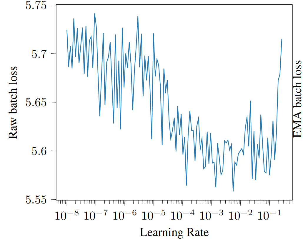
(a) Raw

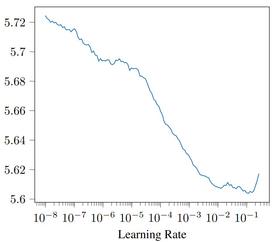
(b) Smoothed

Figure 2: Learning rate finder output (EMA = Exponential Moving Average)

Since the appropriate learning rate is affected by the dataset and architecture, we decided to implement a learning rate finder, in order to be able to get LR upper bounds to use with custom schedules. We could not find a ready-made JAX implementation, so we wrote our own. It is loosely based on the approach described in [Smi17], implemented in the fastai library [How+18]. The learning rate is increased exponentially (as in fastai, and unlike in [Smi17], where the increase is linear) over one epoch; the maximum usable learning rate is then chosen as the maximum value before which the loss stagnates or increases. When it starts exploding, the graph is automatically truncated for readability. See Figure 2. We used this tool pervasively in our notebooks throughout the rest of our experiments.

One we had a learning rate finder, we started experimenting with various schedules, trying to achieve super-convergence [ST18]. We tried a cosine schedule, but noticed that its peaks hurt the network’s performance. We eventually settled for an exponentially-decayed cosine schedule, with a period of one-fifth of the total training time, and a half-life of half the total training time. We observed significantly lower (on the order of 50% lower) training and test set losses with this setup when training over 50 epochs, compared to the one-cycle schedule used in [Zai+19], and accordingly lower guessing entropy. We were able to do so even at a batch size of 400 (with which we scaled the learning rate linearly), with across 8 GPUs.

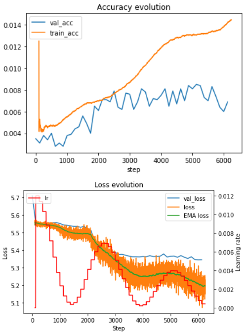
Figure 3: Training plot of our reimplementation of [Zai+19]’s best CNN in the synchronized cast on ASCADv1. The bidirectional impact of the learning rate on the network’s ability to learn can be seen. "EMA loss" is an exponential moving average of the training loss to account for its high variance across batches.

We plot the network’s training curve using this schedule on Figure 3.

2.3 Is Categorical Cross-Entropy the right loss function?

While running experiments, we noticed a peculiar phenomenon, which was also described in [Lu+21]: it is possible for our networks to keep improving with regards to their guessing entropy, while the validation loss goes up and the training loss goes down - which would normally indicate overfitting.

We hypothesize that this is due to categorical cross-entropy being an inadequate choice of loss function for the problem at hand. It does not adequately model the impact of outliers on the final guess, nor of the importance of the relative order of guesses, moreso than the raw magnitude of their log likelihood.

We found the proposal in [Zai+20] of a loss function specifically tailored to the SCA context alluring, but ran into issues when trying to reproduce results using the project’s GitHub repository, as the code could not run as-is. Due to time constraints, we did not attempt to port it to JAX.

2.4 Training Transformers

A list of Transformer architectures we explored was given above. The tests conducted with them were particularly resource-intensive, always requiring us to use as many GPUs as possible in parallel in order to get feedback at an acceptable pace.

Perceiver IO

Adapting Perceiver IO [Jae+21] was relatively straightforward, as the project’s GitHub repository comes with an encoder suited for audio processing that we were able to repurpose. As the model is known to be able to directly attend to individual pixels in the ImageNet setting, we used patches of size 1. We used Fourier positional encoding with 64 bands, as well as learnable encoding of a comparable size. We initially used the project’s default optimizer settings and learning rate scheduling scheme. As the loss did not decrease to a satisfactory value, even on the training set, we lowered the dropout rate to 0 and attempted various maximum learning rates, to no avail: we still observed no convergence with Fourier embeddings. The model did, however, converge with learnable embeddings, but with poor generalization.

Performer

For Performer [Cho+21], we extracted the FAVOR+ mechanism (of which an implementation was published by Google) and built our own Transformer on top of it. We used two to six Transformer blocks, with four to eight heads, and a query/key/value size of 64 to 128. For input embedding, we either extracted patches of the input traces as-is, or used a shallow set of convolutional layers to encode them. Once again, Fourier embeddings positional were ineffective. With learnable positional embedding, the model did learn on the training set, but did not generalize to the validation set within 50 epochs.

Audiomer

We did a summary test with the Audiomer [Sah+22] architecture. Because of tight coupling between the model’s architecture and its input size, we could not adapt it to our 1400-dimensional traces in a straightforward way. As a result, we resampled the traces to the length of 8192 timesteps expected by the model. The model’s loss diverged with its default precision, which used 16-bit floats. With 32-bit floats, it remained stable. However, we found that, with other parameters left at default values and a max learning rate of $10^{-3}$, the model did not learn to be better than a random classifier after 300 epochs, even on the training set. We realize that resampling may have introduced artefacts, but the lack of convergence may also indicate that regularization was too strong (with a dropout rate of 0.2), or that the model’s complexity was too low.

In spite of our efforts, the results we obtained were not encouraging. Given our previous observations regarding the difficulty of achieving convergence, it seems that application of this family of models to the problem may be ineffective without careful architectural considerations, and further hyperparameter tuning with regards to the length of the optimizer’s warm-up period, the weight decay factor, Adam/LAMB’s $\beta_{1}$ and $\beta_{2}$ parameters, the dropout rate, etc. This is especially likely as Transformers are known to be inherently delicate to train [PB18].

3 Conclusion and future work

We developed our own software project to perform Side-Channel Attacks with deep learning using JAX. With it, we were able to reproduce architectures proposed in [Ben+20] and [Zai+19]. We optimized aspects of the training process, such as learning rate scheduling, and conducted our own data exploration (gradient visualization, signal-to-noise analyses). We discovered that [Zai+19]’s models did not generalize to a methodologically-rigorous setting in which the key is unknown on the attack dataset. We tried applying various Transformer-based models on the ASCADv1 variable-key dataset, with limited success.

More careful input preprocessing may be required in order to apply Transformers to the SCA context. We encourage the investigation of techniques such as STFTs, especially for high-resolution and raw traces, as spectral representation is often advantageous for deep learning in a signal-processing context [GCG21, Ell+21]. We also highlight wavelet decomposition [Deb+12] as a possible lead to follow.

In parallel, instead of trying to port the problem to a full Transformer architecture, we suggest trying to incorporate attention gradually into state-of-the-art SCA models. We did not have time to pursue our original goal of building directly upon [Lu+21]; similarly to the approach detailed in it, we suggest attempting to use a locally-connected layer as a means of embedding individual clocks cycles before feeding them to a Transformer.

Code Availability

Our code was made available to the team we worked with at Telecom Paris’s LTCI, in the form of a private GitHub repository and corresponding environment on the Jean Zay platform, so that it may be used for further research.

Update History

The primary content of this manuscript was completed on February 3, 2022, and originally appeared on the website of the institution’s Embedded Systems Concentration. Any revisions after this date pertain to formatting and minor corrections.

References

- [AC21] ANSSI and CEA “ASCAD: Side Channels Analysis and Deep Learning”, 2019-2021 URL: https://github.com/ANSSI-FR/ASCAD
- [Ben+18] Ryad Benadjila, Victor Lomné, Emmanuel Prouff and Thomas Roche “Secure AES128 Encryption Implementation for ATmega8515”, 2018 URL: https://github.com/ANSSI-FR/secAES-ATmega8515
- [Ben+20] Ryad Benadjila et al. “Deep learning for side-channel analysis and introduction to ASCAD database” In Journal of Cryptographic Engineering 10, 2020 DOI: 10.1007/s13389-019-00220-8
- [Bra+18] James Bradbury et al. “JAX: composable transformations of Python+NumPy programs”, 2018 URL: http://github.com/google/jax
- [Bro+20] Tom B. Brown et al. “Language Models are Few-Shot Learners”, 2020 arXiv:2005.14165 [cs.CL]
- [Cho+21] Krzysztof Choromanski et al. “Rethinking Attention with Performers”, 2021 arXiv:2009.14794 [cs.LG]
- [Com] ASCAD Community “Issue 13 - Difference of Datasets: Sampling Frequency / EM & Power?” Accessed: 2022-02-01 URL: https://archive.is/CMSAL
- [Deb+12] Nicolas Debande et al. “Wavelet transform based pre-processing for side channel analysis” In Proceedings - 2012 IEEE/ACM 45th International Symposium on Microarchitecture Workshops, MICROW 2012, 2012, pp. 32–38 DOI: 10.1109/MICROW.2012.15
- [Dev+19] Jacob Devlin, Ming-Wei Chang, Kenton Lee and Kristina Toutanova “BERT: Pre-training of Deep Bidirectional Transformers for Language Understanding”, 2019 arXiv:1810.04805 [cs.CL]
- [DLV03] Pierre Dusart, Gilles Letourneux and Olivier Vivolo “Differential fault analysis on AES” In International Conference on Applied Cryptography and Network Security, 2003, pp. 293–306 Springer
- [Dos+21] Alexey Dosovitskiy et al. “An Image is Worth 16x16 Words: Transformers for Image Recognition at Scale”, 2021 arXiv:2010.11929 [cs.CV]
- [Ell+21] David Elliott, Carlos E. Otero, Steven Wyatt and Evan Martino “Tiny Transformers for Environmental Sound Classification at the Edge”, 2021 arXiv:2103.12157 [cs.SD]
- [Fum+10] Guillaume Fumaroli, Ange Martinelli, Emmanuel Prouff and Matthieu Rivain “Affine Masking against Higher-Order Side Channel Analysis” https://ia.cr/2010/523, Cryptology ePrint Archive, Report 2010/523, 2010
- [GCG21] Yuan Gong, Yu-An Chung and James Glass “AST: Audio Spectrogram Transformer”, 2021 arXiv:2104.01778 [cs.SD]
- [GST17] Daniel Genkin, Adi Shamir and Eran Tromer “Acoustic cryptanalysis” In Journal of Cryptology 30.2 Springer, 2017, pp. 392–443
- [He+15] Kaiming He, Xiangyu Zhang, Shaoqing Ren and Jian Sun “Deep Residual Learning for Image Recognition”, 2015 arXiv:1512.03385 [cs.CV]
- [Hen+20] Tom Hennigan, Trevor Cai, Tamara Norman and Igor Babuschkin “Haiku: Sonnet for JAX”, 2020 URL: http://github.com/deepmind/dm-haiku
- [Hes+20] Matteo Hessel et al. “Optax: composable gradient transformation and optimisation, in JAX!”, 2020 URL: http://github.com/deepmind/optax
- [How+18] Jeremy Howard “The fastai deep learning library” GitHub, https://github.com/fastai/fastai, 2018
- [IS15] Sergey Ioffe and Christian Szegedy “Batch Normalization: Accelerating Deep Network Training by Reducing Internal Covariate Shift”, 2015 arXiv:1502.03167 [cs.LG]
- [Izm+19] Pavel Izmailov et al. “Averaging Weights Leads to Wider Optima and Better Generalization”, 2019 arXiv:1803.05407 [cs.LG]
- [Jae+21] Andrew Jaegle et al. “Perceiver IO: A General Architecture for Structured Inputs and Outputs”, 2021 arXiv:2107.14795 [cs.LG]
- [Jae+21a] Andrew Jaegle et al. “Perceiver: General Perception with Iterative Attention”, 2021 arXiv:2103.03206 [cs.CV]
- [KB17] Diederik P. Kingma and Jimmy Ba “Adam: A Method for Stochastic Optimization”, 2017 arXiv:1412.6980 [cs.LG]
- [KKL20] Nikita Kitaev, Łukasz Kaiser and Anselm Levskaya “Reformer: The Efficient Transformer”, 2020 arXiv:2001.04451 [cs.LG]
- [Koc96] Paul C Kocher “Timing attacks on implementations of Diffie-Hellman, RSA, DSS, and other systems” In Annual International Cryptology Conference, 1996, pp. 104–113 Springer
- [LC19] Guillaume Lample and François Charton “Deep Learning for Symbolic Mathematics”, 2019 arXiv:1912.01412 [cs.SC]
- [Lu+21] Xiangjun Lu et al. “Pay Attention to Raw Traces: A Deep Learning Architecture for End-to-End Profiling Attacks” In IACR Transactions on Cryptographic Hardware and Embedded Systems 2021.3, 2021, pp. 235–274 DOI: 10.46586/tches.v2021.i3.235-274
- [MDP19] Loïc Masure, Cécile Dumas and Emmanuel Prouff “Gradient Visualization for General Characterization in Profiling Attacks” In Constructive Side-Channel Analysis and Secure Design - 10th International Workshop, COSADE 2019, Darmstadt, Germany, April 3-5, 2019, Proceedings 11421, Lecture Notes in Computer Science Springer, 2019, pp. 145–167 DOI: 10.1007/978-3-030-16350-1\_9
- [MS21] Loïc Masure and Rémi Strullu “Side Channel Analysis against the ANSSI’s protected AES implementation on ARM” https://ia.cr/2021/592, Cryptology ePrint Archive, Report 2021/592, 2021
- [PB18] Martin Popel and Ondřej Bojar “Training Tips for the Transformer Model” In The Prague Bulletin of Mathematical Linguistics 110.1 Charles University in Prague, Karolinum Press, 2018, pp. 43–70 DOI: 10.2478/pralin-2018-0002
- [Rad+19] Alec Radford et al. “Language models are unsupervised multitask learners” In OpenAI blog 1.8, 2019, pp. 9
- [RD20] Mark Randolph and William Diehl “Power side-channel attack analysis: A review of 20 years of study for the layman” In Cryptography 4.2 Multidisciplinary Digital Publishing Institute, 2020, pp. 15
- [RT19] Emmanuel Prouff Ryad Benadjila and Adrian Thillar “Hardened Library for AES-128 encryption/decryption on ARM Cortex M4 Achitecture”, 2019 URL: https://github.com/ANSSI-FR/SecAESSTM32/
- [Sah+22] Surya Kant Sahu, Sai Mitheran, Juhi Kamdar and Meet Gandhi “Audiomer: A Convolutional Transformer For Keyword Spotting”, 2022 arXiv:2109.10252 [cs.LG]
- [Smi17] Leslie N. Smith “Cyclical Learning Rates for Training Neural Networks”, 2017 arXiv:1506.01186 [cs.CV]
- [Smi18] Leslie N. Smith “A disciplined approach to neural network hyper-parameters: Part 1 – learning rate, batch size, momentum, and weight decay”, 2018 arXiv:1803.09820 [cs.LG]
- [ST18] Leslie N. Smith and Nicholay Topin “Super-Convergence: Very Fast Training of Neural Networks Using Large Learning Rates”, 2018 arXiv:1708.07120 [cs.LG]
- [SZ15] Karen Simonyan and Andrew Zisserman “Very Deep Convolutional Networks for Large-Scale Image Recognition”, 2015 arXiv:1409.1556 [cs.CV]
- [Sze+15] Christian Szegedy et al. “Rethinking the Inception Architecture for Computer Vision”, 2015 arXiv:1512.00567 [cs.CV]
- [Vas+17] Ashish Vaswani et al. “Attention Is All You Need”, 2017 arXiv:1706.03762 [cs.CL]
- [Wu+21] Haiping Wu et al. “CvT: Introducing Convolutions to Vision Transformers”, 2021 arXiv:2103.15808 [cs.CV]
- [YGG17] Yang You, Igor Gitman and Boris Ginsburg “Large Batch Training of Convolutional Networks”, 2017 arXiv:1708.03888 [cs.CV]
- [You+20] Yang You et al. “Large Batch Optimization for Deep Learning: Training BERT in 76 minutes”, 2020 arXiv:1904.00962 [cs.LG]
- [Zai+19] Gabriel Zaid, Lilian Bossuet, Amaury Habrard and Alexandre Venelli “Methodology for Efficient CNN Architectures in Profiling Attacks” In IACR Transactions on Cryptographic Hardware and Embedded Systems 2020.1, 2019, pp. 1–36 DOI: 10.13154/tches.v2020.i1.1-36
- [Zai+20] Gabriel Zaid et al. “Ranking Loss: Maximizing the Success Rate in Deep Learning Side-Channel Analysis” In IACR Transactions on Cryptographic Hardware and Embedded Systems 2021.1, 2020, pp. 25–55 DOI: 10.46586/tches.v2021.i1.25-55