Magnetic instability and spin-glass order beyond the Anderson-Mott transition in interacting power-law random banded matrix fermions

Abstract

In the presence of quenched disorder, the competition between local magnetic-moment formation and Anderson localization for electrons at a zero-temperature, metal-insulator transition (MIT) remains a long unresolved problem. Here, we study the interplay of these ingredients in a power-law random banded matrix model of spin-1/2 fermions with repulsive Hubbard interactions. Focusing on the regime of weak interactions, we perform both analytical field theory and numerical self-consistent Hartree-Fock numerical calculations. We show that interference-mediated effects strongly enhance the density of states and magnetic fluctuations upon approaching the MIT from the metallic side. These are consistent with results due to Finkel’stein obtained four decades ago. Our numerics further show that local moments nucleate from typical states at the Fermi energy near the MIT, with a density that grows continuously into the insulating phase. We identify spin-glass order in the insulator by computing the overlap distribution between converged Hartree-Fock mean-field moment profiles. Our results indicate that itinerant interference effects can morph smoothly into moment formation and magnetic frustration within a single model, revealing a common origin for these disparate phenomena.

I Introduction

Metal-insulator transitions (MITs) in impure quantum materials present a many-faceted puzzle, with important roles played by Coulomb interactions, magnetic fluctuations, and Anderson localization. Thermodynamic observables such as the spin susceptibility can be enhanced upon approaching the MIT in doped semiconductors [1]; this has been interpreted as evidence for the proliferation of unscreened local magnetic moments [2, 3, 4, 5, 6]. These can nucleate even on the metallic side for sufficiently strong interactions [2, 3]. At the same time, long wavelength quantum interference effects give rise to Anderson localization [7], which is a crucial ingredient for transport properties. The advent of both components suggests a “two-fluid” picture for itinerant electrons and local magnetism, similar to heavy-fermion physics [1, 6, 8].

A strong interplay between magnetism and localization was theoretically suggested four decades ago in calculations performed by Finkel’stein [9]. Using a field theory framework that incorporates interference effects between hydrodynamic modes of the interacting electron liquid, Finkel’stein identified an apparent magnetic instability upon approaching the MIT from the metallic side [10, 4, 11, 12]. Similar to the predicted enhancement of the pairing amplitude near the superconductor-insulator transition [13, 14, 15], itinerant spin-exchange interactions get boosted near the MIT because quantum-critical eigenstates [16] exhibit large spatial overlap and strong state-to-state correlations (“Chalker scaling” [17, 18, 19]). However, the precise nature of the resulting instability and any incipient order has remained controversial [4]. Possible interpretations included nucleation of local moments, itinerant ferromagnetic order [20, 21, 22], or magnetic droplet formation [23]. In the 1990s, these issues were reignited by the observation of a 2D MIT [24, 25, 26, 27, 28]. Competing theories proposed to explain the phenomenon are still under debate [29, 30, 31, 32, 33, 34]. Again magnetic anomalies near the critical point were observed [35, 36, 37], possibly linked to the formation of local moments or spin droplets [38, 39, 40].

In this paper, we seek to clarify the theoretical situation, at least in a particular concrete model. We study spin-1/2 fermions with repulsive Hubbard interactions and power-law random-banded matrix (PRBM) hopping. Noninteracting PRBM models describe fermions with long-ranged random hopping in 1D, and exhibit a well-understood Anderson MIT as a function of the hopping power law [41, 42, 16]. We employ complementary analytical and numerical tools to study the interacting model. Using a Keldysh version of the Finkel’stein field theory [43, 44, 45], we calculate quantum corrections to observables on the metallic side and at the transition. We find an enhanced low-energy density of states, antilocalizing corrections to transport, and a boost to the magnetic susceptibility; these diverge logarithmically with decreasing temperature at the MIT. The obtained results are qualitatively identical to those of Finkel’stein in $d=2+\epsilon$ dimensions [9, 4], indicating some type of magnetic instability near the transition.

We also perform self-consistent Hartree-Fock numerics [46, 47], for which we are able to reach large system sizes (8000 sites). We confirm the analytical results on the metallic side. In addition, the numerics reveals the proliferation of local magnetic moments that begins near the MIT. The moment density grows monotonically as we tune into the insulator, quickly converging with system size. The moments form irregular frozen patterns, with no net ferromagnetic or antiferromagnetic character. We calculate overlaps between different mean-field converged spin configurations. The distribution function that we obtain is reminiscent of full replica symmetry breaking in infinite-range spin glasses [48, 49].

Thus we find that both long-wavelength interference effects and local-moment physics play crucial roles in the same model, albeit on opposite sides of the MIT. Our most interesting finding is that local moments appear to smoothly emerge from the quantum-critical, mulitifractal-enhanced state that characterizes the MIT, suggesting a single-fluid model whose character changes from itinerant to localized at the MIT. I.e., this is a full many-body localization transition at zero temperature. A key question for future research is whether this dual character of the interacting, disordered fluid survives correlation effects beyond the Hartree-Fock framework employed here.

This paper is organized as follows. In Sec. II, we summarize the main analytical and numerical results. Analytical results for the density of states (DOS), MIT, and spin susceptibility are presented in Sec. II.2. Numerical results for the DOS, moment formation, spin susceptibility, and evidence for spin-glass order are presented in Sec. II.3. Additional technical details on the self-consistent mean-field numerics for the PRBM-Hubbard model are given in Sec. III. We set up the long-wavelength field theory description of the interacting PRBM model and derive quantum corrections in Sec. IV. In Sec. V, we conclude and discuss the outlook for future research.

II Summary of main results

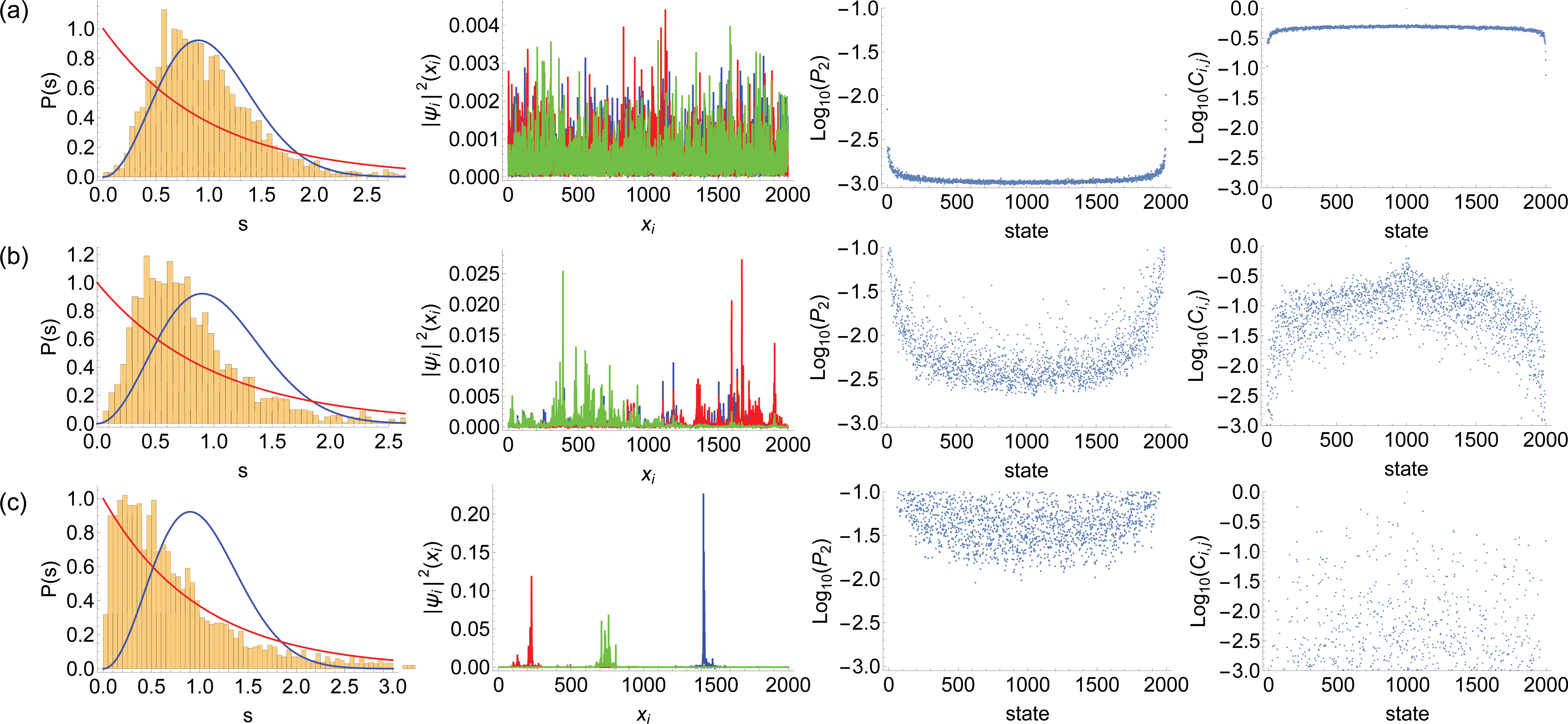
Figure 1: Key features of the non-interacting GUE-PRBM model [Eq. (2.1) with $U$ = 0], from the ergodic to Anderson-localized regimes. Numerical results are shown from exact diagonalization of an $L=2000$ site system (single disorder realization), with (a) $\alpha=0.5$ (ergodic phase), (b) $\alpha=1.0$ (Anderson MIT), and (c) $\alpha=1.3$ (Anderson insulator). From left to right each row depicts (i) the level statistics, (ii) probability profiles in position space for 3 consecutive mid-spectrum eigenstates, (iii) the IPR $P_{2}$ [Eq. (2.4)] versus state number, and (iv) the Chalker correlator $C_{i,j}$ [Eq. (2.5)] for the mid-spectrum state $i=1000$ versus the state $j$. The blue (red) curve for the level statistics is the GUE Wigner surmise [52] (Poisson distribution). The IPR $P_{2}$ is small [${\mathit{O}}\left(1/L\right)$] for almost all states in the ergodic phase, but becomes substantial in the Anderson insulator. The Chalker correlator takes a flat nonzero value for ergodic states, shows power-law dependence in state number at the MIT [Chalker scaling, Eq. (2.6)], but is strongly suppressed in the insulator (except for discrete states residing in the same localization volume as the selected state). For all results presented here, we have chosen $b=1$ [Eq. (2.3)].

We consider an SU(2)-invariant spin-$1/2$ PRBM model with repulsive Hubbard interactions,

$$H=\sum_{ij,s}\mathsf{H}_{ij}c^{\dagger}_{is}c_{js}+U\sum_{i}n_{i\uparrow}n_{i\downarrow}-\mu\sum_{i}n_{i}.$$ (2.1)

Here $c_{js}$ annihilates a spin-$s\in\{\uparrow,\downarrow\}$ fermion at site $x_{j}$, and $\mathsf{H}_{ij}=\mathsf{G}_{ij}\,a\left(\left|i-j\right|\right)$, where $\mathsf{G}_{ij}$ denotes a random matrix in the Gaussian unitary ensemble. We set the energy variance of the Gaussian random matrix to one,

$$\overline{\mathsf{G}_{ij}\,\mathsf{G}_{kl}}=\left(\Delta\mathsf{G}\right)^{2}\delta_{il}\,\delta_{kj},\qquad\Delta\mathsf{G}=1,$$ (2.2)

where the overline denotes disorder averaging. The Hubbard interaction strength $U$ is then dimensionless, measured in units of the standard deviation $\Delta\mathsf{G}$. In Eq. (2.1), $a\left(\left|i-j\right|\right)$ is an envelope function modulating the hopping that decays as $|i-j|^{-\alpha}$ at large distances,

$$a\left(\left|i-j\right|\right)=\begin{cases}1&|i-j|<b\,,\\ \left|\frac{i-j}{b}\right|^{-\alpha}&|i-j|\geq b\,.\end{cases}$$ (2.3)

We have set the lattice constant equal to one; the length parameter $b$ is discussed below.

In this section, we summarize the main results of this paper. In Sec. II.1 we first review key aspects of the noninteracting PRBM model, Eq. (2.1) with $U=0$. In Sec. II.2, we present analytical results regarding the interacting MIT. We employ the non-linear sigma model [9, 4, 11] description of Eq. (2.1) that incorporates density-density and spin-triplet fermion interactions, which descend from the Hubbard $U$. Perturbation theory in the sigma model is controlled for large $b\gg 1$ [41, 42, 16]. We obtain very similar results to those in $d=2+\epsilon$ dimensions [9, 4]: Altshuler-Aronov effects increase the density of states, transport, and spin susceptibility, due to enhanced spin-triplet interactions.

In Sec. II.3, we follow up with mean-field (Hartree-Fock) exact diagonalization numerics for Eq. (2.1) with $b=1$ [Eq. (2.3)]. The results on the metallic side and at the MIT are consistent with the analytical picture. With numerics, however, we are able to penetrate the interacting Anderson insulating regime. There we observe the nucleation of a small density of local magnetic moments. The nucleation proceeds smoothly as we tune away from the MIT, with unpaired spins forming from typical localized states near the Fermi energy. We present evidence that these moments form a spin glass. This is interesting because it suggests that replica symmetry breaking [48, 49] is necessary to capture the physics on the insulating side of the interacting MIT. By contrast, NLsM studies typically presume replica-symmetric ansätze in both the metallic and insulating regimes [50].

II.1 Review of the non-interacting PRBM model

The noninteracting PRBM model exhibits three different regimes, depending upon the exponent $\alpha$. For $0\leq\alpha<1/2$, the physics is similar to the random-matrix limit $\alpha=0$. Level statistics are determined by the Wigner surmise [52, 53], and wave functions are extended and featureless. For $1/2<\alpha<1$, the wave functions are ergodic, but exhibit strong fluctuations in finite size. The Anderson MIT at $\alpha=1$ is “spectrum-wide critical,” in that almost all wave functions except those in the Lifshitz tails become critical (multifractal [41, 42, 16]). For $\alpha>1$, all states Anderson localize and level statistics cross over to the Poisson distribution.

Extended and localized states can be distinguished by the inverse participation ratio (IPR) [16],

$$P_{2}(\psi_{i})\equiv\sum_{x}\left|\psi_{i}(x)\right|^{4}.$$ (2.4)

For an extended (critical) eigenfunction $\psi_{i}$, $P_{2}\sim(1/L)^{\tau_{2}}$ with $\tau_{2}=1$ ($0<\tau_{2}<1$); here $L$ denotes the system size. A localized state with a localization length smaller than $L$ instead has $\tau_{2}=0$ and $P_{2}\sim{\mathit{O}}\left(1\right)$. We note that there are small finite-size power-law corrections to $P_{2}$ even in the insulator, due to Lévy flights [16, 54].

Another way to characterize the system is via the Chalker correlator

$$C_{ij}\equiv 2\,\frac{\sum_{x}\left|\psi_{i}(x)\right|^{2}\left|\psi_{j}(x)\right|^{2}}{P_{2}(\psi_{i})+P_{2}(\psi_{j})}.$$ (2.5)

This is a normalized, “energy-split” IPR that measures the degree of spatial overlap between the position-space distribution functions of two different eigenstates. In the ergodic phase $C_{ij}$ is a constant for $i\neq j$. In the Anderson insulator $C_{ij}$ is strongly suppressed except for a discrete set of eigenenergies, because localized states that are nearby in energy are typically far-separated in position space. At the Anderson MIT, one expects power-law scaling [17, 18, 19, 13]

$$C_{ij}\sim|\varepsilon_{i}-\varepsilon_{j}|^{\tau_{2}/d-1},$$ (2.6)

where $d$ is the number of spatial dimensions. Although individual critical eigenstates consist of self-similar ensembles of rare, well-separated peaks, these peaks strongly overlap for states with nearby energies, in sharp contrast to the Anderson insulator. See the second and fourth panels of Fig. 1(b). This critical scaling can enhance matrix elements of interactions [13, 14, 15, 55, 56]. It has been predicted to boost the pairing amplitude near the superconductor-insulator transition, in the absence of long-ranged Coulomb interactions [13, 14, 15, 57].

In Fig. 1, we exhibit numerical results for a GUE-PRBM model and three different values of $\alpha$. Results are presented for level statistics, representative wave functions, and spectrum-wide statistics for the IPR [Eq. (2.4)] and Chalker correlator [Eq. (2.5)].

For $1/2<\alpha<3/2$, the PRBM model can be mapped to a 1D version of the standard field theory of noninteracting localization, the non-linear sigma model (NLsM) [41, 42, 16]. The theory is identical to the usual one, except that the gradient-squared term is replaced by a nonlocal power of momentum $|k|^{\sigma}$, where $\sigma=2\alpha-1$. This leads to superballistic transport throughout the ergodic phase $0\leq\sigma<1$. The theory becomes renormalizable at the MIT, where $\sigma=1$.

The DOS per spin of the GUE-PRBM model is well-approximated by the saddle-point of the sigma model, which gives a generalized Wigner semicircle law

$$\nu\left(\omega\right)=\frac{1}{\pi J_{0}}\sqrt{J_{0}-\frac{\omega^{2}}{4}}\,,$$ (2.7)

with $J_{0}=\sum_{j}J_{ij}$ and $J_{ij}=a^{2}\left(\left|i-j\right|\right)$. With the form of $a\left(\left|i-j\right|\right)$ given by Eq. (2.3), we have

$$J_{0}=2b^{2\alpha}\left[\zeta\left(2\alpha,b\right)-\zeta\left(2\alpha,L/2\right)\right]+2b-1\,.$$ (2.8)

Here $\zeta(a,x)$ is the Hurwitz zeta function and $L$ is the system size. The DOS in Eq. (2.7) is compared to numerics for variable $\alpha$ in Fig. 3(a). In the random-matrix regime $-1\leq\sigma<0$, the range of the energy spectrum increases with system size as $\sim L^{-\sigma/2}$ and the zero-energy DOS (at the spectrum center) decreases with system size $\sim L^{\sigma/2}$. For $\alpha>1/2$ ($\sigma>0$), the DOS becomes system-size independent, up to finite-size corrections $\sim L^{-\sigma/2}$. The range of the energy spectrum (peak of the DOS) decreases (increases) with increasing $\alpha$.

II.2 Analytical results: Magnetic instability

To treat the effects of the interactions in the PRBM-Hubbard model in Eq. (2.1), we derive the the interacting (Finkel’stein) version of the NLsM [9, 4]. We work at half-filling throughout this paper. Using the Keldysh formalism [43, 44, 45], we incorporate two effective dimensionless interaction parameters: a density-density coupling $\gamma_{s}>0$, and a spin-triplet interaction $\gamma_{t}<0$. For $U>0$, the density-density (spin-triplet) interaction is repulsive (attractive) [4, 8].

The dimensionless effective parameters $\gamma_{s,t}$ incorporate Fermi-liquid renormalizations [9]. The limit $\gamma_{t}\rightarrow-\infty$ would correspond to the Stoner instability to ferromagnetism in a clean system. Calculations performed four decades ago for the diffusive, interacting Fermi liquid in $d=2+\epsilon$ dimensions predicted some kind of magnetic instability, signaled by the runaway RG flow of $\gamma_{t}$ towards negative infinity [9, 10, 4]. Due to the antilocalizing effects of $\gamma_{t}$-mediated Altshuler-Aronov corrections, this instability was predicted to pre-empt the expected disorder-driven MIT. Despite enormous efforts, the nature of the instability in the field theoretic framework was never fully clarified. Possible interpretations include an interference-enhanced ferromagnetic instability [20, 22, 23], or the formation of localized spin moments [2, 3, 6, 58]. A large-$N$ version of the sigma model was formulated to suppress the intervening magnetic phase, in an attempt to explain the 2D MIT [31, 27].

In this subsection we show that the sigma model predicts a phenomenology for the PRBM-Hubbard model that is very similar to the finite-dimensional results. In particular, the triplet channel enhances the DOS, transport, and the spin susceptibility at the interacting MIT. As with the results in $d=2+\epsilon$ dimensions, the nature of any magnetic order that onsets near the MIT is not determined by the standard perturbative field-theory treatment. In Sec. II.3, below, we instead employ self-consistent numerics to show that local moments form a spin glass in the insulating phase.

II.2.1 Density of states

The DOS receives interference-mediated interaction (Altshuler-Aronov) corrections [7]. Using the NLsM, at the MIT ($\alpha=1$) we obtain

$$\delta\nu=\frac{\nu_{0}\lambda}{2\pi}\left[\ln{\left(1-\gamma_{s}\right)}+3\ln{\left(1-\gamma_{t}\right)}\right]\ln\left({\frac{\Lambda}{T}}\right)\,.$$ (2.9)

Here $\nu_{0}=1/\pi\sqrt{J_{0}}$ is the bare DOS per spin at the Fermi energy, and $\lambda$ is the inverse of the superdiffusive “conductivity” [see Eq. (2.13)], up to a constant. For the PRBM-Hubbard model, $\lambda\propto b^{-1}$ at the MIT [Eq. (4.2)], and serves as the control parameter for perturbation theory when $b\gg 1$. In Eq. (2.9), $\Lambda$ is the ultraviolet (UV) cutoff in energy and the temperature $T$ serves as the infrared (IR) cutoff. Because the repulsive Hubbard $U$ gives $\gamma_{s}>0$ and $\gamma_{t}<0$, the singlet channel interaction suppresses the DOS whilst the triplet one enhances it. Near the MIT, the triplet channel interaction dominates (see below) and the DOS is predicted to be enhanced.

Figure 2: The RG-improved prediction for the DOS of the PRBM-Hubbard model near zero energy [Eq. (2.10)]. The enhancement is due to the Altshuler-Aronov correction in the triplet interaction channel. Here we set $\lambda=0.1$, $\gamma_{t}^{0}=0.1$ and $\Delta=1$.

RG flow equations for $\lambda$, $\nu$ and the interactions can be obtained from the corresponding response functions. Ignoring the singlet coupling $\gamma_{s}$ and the logarithmically slow flow of $\lambda$, near the MIT we obtain the approximate dependence of the DOS close to the Fermi energy,

$$\nu\left(\varepsilon\right)\sim e^{-3\mathsf{Li}_{2}\left[\gamma_{t}^{0}\left(\frac{\Delta}{\varepsilon}\right)^{\lambda}\right]}\,.$$ (2.10)

Here $\varepsilon$ is the energy relative to the Fermi level, $\Delta$ is the UV energy scale ($\sim$ bandwidth), and $\mathsf{Li}_{2}(x)$ is the dilogarithm function. Eq. (2.10) applies over an intermediate range of energies, but cannot be trusted in the limit $\varepsilon\rightarrow 0$; the latter corresponds to the strong coupling regime wherein the perturbative RG must break down. The interaction-enhanced DOS is shown in Fig. 2. The prediction is consistent with the numerical results that we summarize in Sec. II.3, see Fig. 3.

II.2.2 Density dynamics

The semiclassical density-density response function takes the form

$$\Pi^{0}(\omega,k)=-\kappa\frac{D_{c}|k|^{\sigma}}{D_{c}|k|^{\sigma}-i\omega}\,.$$ (2.11)

Here $\sigma=2\alpha-1$ and $\alpha$ is the hopping exponent for the PRBM, $D_{c}$ is the charge superdiffusion constant, and $\kappa$ the charge compressibility,

$$D_{c}\equiv\frac{D}{1-\gamma_{s}}\,,\qquad\kappa\equiv 2\nu_{0}(1-\gamma_{s})\,.$$ (2.12)

The energy superdiffusion constant $D=2/(\lambda\pi\nu_{0})$. Near the MIT ($0<\sigma<2$, $1/2<\alpha<3/2$), the semiclassical electron motion is superdiffusive and the conductivity diverges. Thus, we define the following superdiffusive “conductivity” to characterize transport,

$$\mathfrak{g}\equiv\lim_{k\to 0}\frac{i\omega}{|k|^{\sigma}}\Pi(\omega,k)=\frac{4}{\pi}\lambda^{-1}.$$ (2.13)

In the ergodic phase ($\sigma<1$), the Altshuler-Aronov correction to transport is given by

$$\delta\mathfrak{g}=\frac{2\Lambda_{k}^{1-\sigma}}{\pi^{2}\left(1-\sigma\right)}\left[\ln\left(1-\gamma_{s}\right)+3\ln\left(1-\gamma_{t}\right)\right].$$ (2.14)

Here $\Lambda_{k}$ is the UV cutoff in momentum. The correction is UV divergent (IR convergent), indicating the RG-irrelevance of $\lambda$ in the ergodic regime (similar to the resistivity of a diffusive metal in 3D).

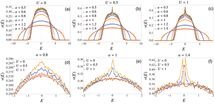
Figure 3: The density of states for PRBM-Hubbard model with repulsive Hubbard interactions. The results are taken for systems of size $L=4000$ and averaged over $N_{\mathsf{ens}}=50$ disorder realizations. The dashed lines indicate the DOS for non-interacting systems obtained via the NLsM [Eq. (2.7)]. The curve at $\alpha=0.5$ is taken to be slightly away to avoid the divergence of Eq. (2.7) at $\alpha=1/2$. Panels (a), (b) and (c) show the DOS for different hopping powers $\alpha$ with $U=0$, $0.5$ and $1$, respectively. Panels (d), (e) and (f) show the DOS for different interaction strength with $\alpha=0.8$, $1$ and $1.4$, respectively. The DOS is not changed by the interaction for systems with $\alpha$ close to $0.5$. When $\alpha$ approaches the MIT, the DOS receives quantum corrections due to the interplay of interactions and critical wave functions. The observed enhancement is consistent with the analytical results due to the Altshuler-Aronov correction in the spin-triplet channel, Eq. (2.10) and Fig. 2. In the localize phase, the DOS near the Fermi energy is still enhanced, but begins to show a dip for stronger interactions $U\gtrsim 1$ due to the crossover towards Mott localization.

At the noninteracting critical point ($\sigma=1$), the dependence on the UV cutoff becomes logarithmic and the correction can be cut off in the infrared by the temperature,

$$\delta\mathfrak{g}=\frac{2}{\pi^{2}}\left[\ln\left(1-\gamma_{s}\right)+3\ln\left(1-\gamma_{t}\right)\right]\ln\left(\frac{\Lambda}{T}\right)\,.$$ (2.15)

Different from the usual case [4], the form of the Altshuler-Aronov corrections in Eqs. (2.9) and (2.15) is identical. This is due to the nonanalytic character of the density fluctuations in the PRBM [Eq. (2.11)]. As a result, only a subset of the usual diagrams that renormalize transport contribute to Eq. (2.15), and these are precisely those responsible for DOS renormalization, see Sec. IV.3.

Eq. (2.15) implies that the singlet (triplet) interaction is localizing (antilocalizing). We find numerically that the interacting MIT is slightly shifted to $\alpha>1$ by moderate Hubbard interactions, see Fig. 11. This is consistent with magnetic fluctuation-dominated antilocalization, which we attribute to the same Altshuler-Aronov effect responsible for the DOS enhancement in Figs. 2 and 3.

II.2.3 Magnetic fluctuations boosted by multifractality

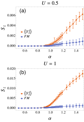
Figure 4: The local moment density $\left\langle\left|S_{i}^{z}\right|\right\rangle$ [Eq. (2.21)] and ferromagnetic order parameter $S^{z}_{\scriptstyle\mathsf{FM}}$ [Eq. (2.20)] for the PRBM-Hubbard model. The data are taken for system of size $L=2000$ and averaged over $N_{\mathsf{ens}}=100$ disorder realizations. Both vanish in the ergodic regime with $0.5\lesssim\alpha\ll 1$, and the mean field ground state is spin unpolarized. Both arise close to the critical point near $\alpha=1$ and increase with $\alpha$ into the localized phase. However, the weak net magnetization does not indicate ferromagnetism. The FM order parameter is much smaller than the local moment density and its variance due to ensemble averaging (error bars in the plot) is comparable to its mean.

The semiclassical spin response function is determined by the dynamical susceptibility

$$\chi_{ij}^{0}\left(\omega,k\right)=\delta_{ij}\chi_{0}\frac{D_{t}|k|^{\sigma}}{D_{t}|k|^{\sigma}-i\omega}\,.$$ (2.16)

Here $D_{t}$ is the spin superdiffusion constant and $\chi_{0}$ is the bare static spin susceptibility,

$$D_{t}\equiv\frac{{D}}{1-\gamma_{t}}\,,\qquad\chi_{0}\equiv 2\nu_{0}\left(1-\gamma_{t}\right)\,.$$ (2.17)

The static spin susceptibility can be extracted from the spin response function in the static limit $\omega\to 0$.

In the ergodic phase with $\sigma<1$, the static spin susceptibility receives a quantum correction,

$$\chi_{ij}=\delta_{ij}\chi_{0}\left[1-\frac{\lambda\gamma_{t}\Lambda_{k}^{1-\sigma}}{\pi\left(1-\sigma\right)}\right]\,.$$ (2.18)

The quantum correction is proportional to $\lambda$, the strength of the triplet-channel interaction $\gamma_{t}$, and the UV cutoff $\Lambda_{k}^{1-\sigma}$. At the critical point, this becomes

$$\chi_{ij}=\delta_{ij}\chi_{0}\left[1-\frac{\lambda\gamma_{t}}{\pi}\ln\left(\frac{\Lambda}{T}\right)\right]\,.$$ (2.19)

Repulsive Hubbard $U$ gives $\gamma_{t}<0$, so that the spin susceptibility is enhanced by quantum interference.

The RG equations for the singlet and triplet interaction strengths near the MIT take the same form as in the original Finkel’stein calculation [9, 59] in $d=2+\epsilon$ dimensions, see Eq. (4.61). These equations possess a single relevant direction that leads to the runaway RG flow of $\gamma_{t}\rightarrow-\infty$. The mechanism that drives the flow away from weak coupling is the multifractal enhancement of matrix elements [13, 14, 15, 55, 56, 57], due to the Chalker scaling of quantum-critical wave functions [Figs. 1(b,d) and Eq. (2.6)]. The divergence of $|\gamma_{t}|$ drives a simultaneous divergence of the spin susceptibility in Eq. (2.19). A susceptibility peak near the MIT can also be discerned in the numerical results presented in the next section, see Fig. 6. These results signal the onset of magnetic phenomena at the MIT, but the standard field-theoretic approach is ill-suited to determine its character.

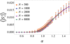
Figure 5: The local moment density $\left\langle\left|S^{z}_{i}\right|\right\rangle$ [Eq. (2.21)] for different system sizes with $U=1$. The $L=500$, $1000$, $2000$ and $4000$ data are averaged over $1000$, $500$, $100$, $50$ and $40$ disorder realizations, respectively. Near the MIT, the onset of $\left\langle\left|S^{z}_{i}\right|\right\rangle>0$ slightly sharpens with system size. The moment density becomes system-size independent in the localized phase and its variance decreases with increasing $L$.

II.3 Self-consistent Hartree-Fock numerics

II.3.1 Local moment formation

The analytical results presented in Sec. II.2 demonstrate the onset of strong magnetic fluctuations near the MIT in the PRBM-Hubbard model. To elucidate the nature of these fluctuations and any incipient order that develops, we turn to Hartree-Fock numerical calculations. We use static mean-field theory to decouple the Hubbard interactions in terms of the onsite magnetization, and perform self-consistent exact diagonalization of the resulting quadratic fermion Hamiltonian. We restrict our attention to mean-field states with collinear magnetic order. Details of the procedure and convergence criteria are discussed in Sec. III. All results presented in this section take $b=1$ in Eq. (2.3). Because perturbation theory formally requires $b\gg 1$, in general we anticipate only qualitative agreement between analytics and numerics.

Fig. 3 shows the density of states in the PRBM model with and without the repulsive Hubbard-$U$ interaction. In the non-interacting case, the numerical DOS [solid lines in Fig. 3(a)] matches well the Wigner semicircle prediction [Eq. (2.7), dashed lines in Figs. 3(a)–(c)], except in the Lifshitz tails near the band edges.

The repulsive Hubbard $U>0$ interaction is found to enhance the numerical DOS near the Fermi surface at zero energy, when the system is tuned through the MIT. Deep in the ergodic phase $\alpha\sim 0.5$, the effect is negligible. Near the interaction-dressed MIT [Fig. 3(e)], a sharp peak appears in the DOS. The peak becomes sharper for moderate interactions ($U\sim 0.5$) as $\alpha$ increases and the system enters the localized phase, see Fig. 3(b). This is consistent with the analytical prediction in Eq. (2.10) and Fig. 2 due to Altshuler-Aronov corrections in the spin-triplet channel, suggesting the onset of strong magnetic fluctuations. For stronger interactions ($U\gtrsim 1$), the enhancement of the DOS persists for states near the Fermi energy in the localized phase; however, a dip appears in the localized system exactly at the Fermi energy [Fig. 3(f)], indicating the crossover towards Mott localization expected with strong Hubbard $U$.

Fig. 4 shows the ferromagnetic (FM) and local magnetic moment density order parameters in the PRBM-Hubbard model. The FM order parameter is evaluated in the Hartree-Fock ground state,

$$S^{z}_{\mathsf{FM}}=\left\langle\frac{1}{2L}\sum_{i}\left(n_{i\uparrow}-n_{i\downarrow}\right)\right\rangle\,.$$ (2.20)

The local moment density is defined via

$$\left\langle\left|S_{i}^{z}\right|\right\rangle=\left\langle\frac{1}{2L}\sum_{i}\left|n_{i\uparrow}-n_{i\downarrow}\right|\right\rangle\,.$$ (2.21)

Here $\left\langle\cdots\right\rangle$ denotes ensemble averaging over different disorder realizations. The local moment density is conceptually similar to the Edwards-Anderson order parameter [60] for spin glasses. Deep in the ergodic phase both $S^{z}_{\mathsf{FM}}$ and $\left\langle\left|S_{i}^{z}\right|\right\rangle$ are negligible. Near the MIT, local moments start to form and $\left\langle\left|S_{i}^{z}\right|\right\rangle$ increases with $\alpha$ in the localized phase. Concomittantly ferromagnetism appears to nucleate and increase with $\alpha\gtrsim 1$. However, the FM magnetization is extremely small, corresponding to a few majority spins, and its variance induced by disorder averaging is comparable to its mean. The net magnetization decreases with increasing system size $L$. For the studied values of $U$, antiferromagnetic order is even weaker, and also suppressed with increasing $L$. By contrast, the local moment density is well-converged with $L$ in the insulating phase, see Fig. 5. The onset $\left\langle\left|S_{i}^{z}\right|\right\rangle>0$ sharpens slightly with increasing $L$ near the MIT $\alpha\sim 1$. Representative moment profiles for a small system and different $\alpha$ are exhibited in Appendix A, Fig. 17. Different initial conditions in the self-consistent Hartree-Fock procedure produce similar spatial profiles for $\left\langle\left|S_{i}^{z}\right|\right\rangle$, but different signs of the localized moments, see Fig. 18 in Appendix A. This is suggestive of spin-glass order, discussed further below.

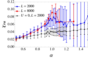
Figure 6: The spin susceptibility in the PRBM-Hubbard model for different system sizes with $U=1$. The $L=2000$ (blue circle) and $L=8000$ (red square) data are averaged with $100$ and $40$ disorder realizations, respectively. The incremental applied field is $\Delta h=0.02$ for $L=2000$ and $\Delta h=0.01$ for $L=8000$. The spin susceptibility can be boosted by the interplay of spin-triplet interactions and multifractality near the MIT, see Eq. (2.19) and the discussion in Sec. II.2.3. The interacting susceptibility is indeed enhanced compared to the non-interacting system (black dashed curve). Near the MIT, the interacting $\chi_{\scriptstyle\mathsf{FM}}$ shows a non-diverging peak. At the same time, the fluctuations induced by ensemble averaging are very large for all $\alpha\gtrsim 1$ in the interacting case, consistent with the absence of ferromagnetism (Fig. 4).

The ferromagnetic spin susceptibility can be obtained via

$$\chi_{\scriptstyle\mathsf{FM}}\left(\Delta h\right)\equiv\lim_{\Delta h\to 0}\frac{S_{\scriptstyle\mathsf{FM}}^{z}\left(\Delta h\right)-S_{\scriptstyle\mathsf{FM}}^{z}\left(-\Delta h\right)}{2\Delta h}\,.$$ (2.22)

In a ferromagnet, the susceptibility should diverge when $\Delta h$ goes to $0$. On the other hand, the spin susceptibility shows a non-diverging cusp near the spin glass transition [48]. In the PRBM-Hubbard model, susceptibility data with very small $\Delta h$ is overshadowed by the fluctuations due to ensemble averaging. The spin susceptibility in Fig. 6 does exhibit a strong enhancement compared to that of the non-interacting system, and a non-diverging peak near the MIT. The peak becomes sharper with increasing systems size. However, the fluctuations of the spin susceptibility (error bars in Fig. 6) across disorder realizations become very large for $\alpha\gtrsim 1$, consistent with the absence of true ferromagnetic order.

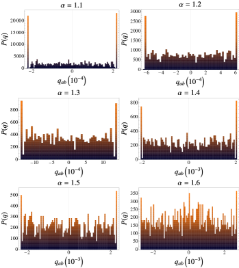
Figure 7: The distribution $P(q)$ [Eq. (2.24)] of the replica symmetry breaking order parameter $q_{ab}$ with $a$ fixed for a particular reference state (converged solution to the self-consistent Hartree-Fock numerics). The initial conditions for each of the replica $b$’s are obtained by flipping the spin configurations of the reference state $a$. In the localized phase, $q_{ab}$ exhibits a bimodal distribution with two peaks at $\pm q_{\scriptstyle\mathsf{max}}$, and the distribution between the two peaks is approximately uniform and nonzero. The probability density of the two bimodal peaks decreases and that between the two peaks increases with increasing $\alpha$, implying weaker correlations between the local moments with decreasing localization length. The Hubbard interaction is $U=1$.

II.3.2 Spin-glass order

A classical equilibrium spin glass exhibits a very large number of nearly-degenerate metastable “pure” states with different spin configurations [49]. These nearly-degenerate states are separated by large free-energy barriers in a complex configuration landscape. Below the spin-glass transition temperature, the system will converge (in dissipative dynamics or simulated annealing) into one of these ergodicity-breaking metastable states.

The mean-field states obtained in self-consistent numerics depend upon the choice of initial conditions in the spin-glass phase. By choosing different initial conditions, we obtain an ensemble of “replicas” (solutions). Since we restrict our attention to collinear solutions of the mean-field equations, we can characterize these in terms of the local magnetization $S^{z}_{i,a}$ profile, where $i$ labels the lattice site and $a$ indexes the replica. Examples drawn from converged solutions in the insulating phase with $\alpha=1.1$ are depicted in Fig. 18, Appendix A. (Convergence criteria and stability for a particular state are discussed in Sec. III.)

A collinear (Ising) spin-glass phase can be characterized by the distribution function for the overlaps $q_{ab}$, defined via

$$q_{ab}\equiv\frac{1}{L}\sum_{i}S_{i,a}^{z}\,S_{i,b}^{z}.$$ (2.23)

Here $a$ and $b$ are indices labeling different replicas and $S^{z}_{i,a}$ is the spin configuration of the converged Hartree-Fock mean-field state in replica $a$. In practice, we chose the replica $a$ as the converged solution for an arbitrary initial condition and take it as the reference state. For each of the replica $b$’s, we sample a random number $r\in[0,1]$ from the uniform distribution. The initial condition for replica $b$ is then obtained by flipping a portion $r$ of the local spin polarization $\{S_{i,a}^{z}\}$ in the solution $a$. The overlap between the initial spin configuration used to seed the calculation for replica $b$ and that of the coverged reference state $a$ is approximately uniform. We then perform self-consistent numerics with the modified initial condition and obtain the final spin configuration $\{S^{z}_{i,b}\}$ for replica $b$. With self-consistency, the distribution of the overlaps between the converged solutions $\{b\}$ and that of the reference state $a$ deviates from the uniform distribution and shows spin-glass characteristics.

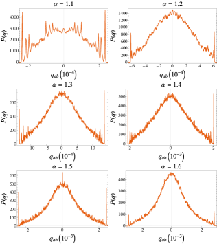
Figure 8: The distribution $P(q)$ [Eq. (2.25)] of the replica symmetry breaking order parameter $q_{ab}$ between all the replicas. The ensembles of the replicas are chosen in the same way as that in Fig. 7. The distribution functions show two sharp peaks at $\pm q_{\scriptstyle\mathsf{max}}$ and another smooth peak at $q=0$. The peaks at $\pm q_{\scriptstyle\mathsf{max}}$ characterize the spin glass order and their values decrease with increasing $\alpha$. The smooth peak at $q=0$ results from the choice of the replica ensemble (set of initial conditions for the self-consistent numerics).

The spin-glass order is characterized by the distribution of the overlaps $q_{ab}$. Fig. 7 shows the distribution function of $q_{ab}$ defined via

$$P(q)\equiv\sum_{b}\delta(q-q_{ab})\,.$$ (2.24)

Here we fix the replica $a$ as the reference state and sum over all the replica $b$’s. The $q_{ab}$ in Fig. 7 with fixed $a$ shows a bimodal distribution in the localized phase ($\alpha>1$). Two peaks appear in the distribution at $\pm q_{\scriptstyle\mathsf{max}}$, reflecting the spin $\text{SU}(2)$ symmetry of the PRBM-Hubbard model. Between the two peaks, the distribution is approximately uniform, but with a probability density smaller than that in the distribution of overlaps between the reference state $a$ and the initial conditions seeding the calculation of the replica $b$’s. With increasing $\alpha$, $q_{\scriptstyle\mathsf{max}}$ increases and the peak value at $\pm q_{\scriptstyle\mathsf{max}}$ of the distribution function decreases. At large $\alpha$ ($\alpha>1.5$), the localization length of the single-particle wave functions is reduced to the order of the lattice constant. As a result, the correlations between the local moments become much weaker and the spin-glass order is strongly diminished. The distribution of overlaps between the converged replica solutions becomes closer to the uniform distribution of the initial conditions, with much lower peaks at $\pm q_{\scriptstyle\mathsf{max}}$.

Fig. 8 shows the replica ensemble-averaged distribution function,

$$P(q)=\sum_{a,b}\delta(q-q_{ab})\,.$$ (2.25)

Here the replicas are still chosen in the same way as previously stated, but we consider the distribution of the overlap between all of the replicas, rather than the overlap with a single reference state. The bimodal distribution of the spin glass order is still clear with two peaks at $\pm q_{\scriptstyle\mathsf{max}}$.

The distribution of overlaps exhibited in Fig. 7 is qualitatively similar to the continuous Parisi replica-symmetry breaking solution for the classical Ising Sherrington-Kirkpatrick model [49]; a similar ansatz obtains for the classical isotropic Heisenberg glass [48]. Combined with the direct inspection of converged Hartree-Fock solutions shown in Figs. 17 and 18, we conclude that the interacting Anderson insulator exhibits spin-glass order. Spin-glass order cannot be ascertained via the field-theory calculations presented in Sec. II.2, which expand around a replica-symmetric saddle-point.

We note that classical spin-glass models with power-law interactions were investigated long ago [61, 62, 63, 48]. The Hamiltonian takes the form

$$H=\sum_{i<j}\frac{\epsilon_{ij}\,\sigma_{i}\,\sigma_{j}}{|i-j|^{\Upsilon}}.$$ (2.26)

Here $\sigma_{i}\in\pm 1$ is an Ising variable, and $\{\epsilon_{ij}\}$ are taken to be identically distributed, independent Gaussian random variables with zero mean. This model exhibits a finite-temperature spin-glass transition only for $\Upsilon<1$, with non-mean-field exponents in the window $2/3<\Upsilon<1$. However, we stress that the effective spin exchange induced in the self-consistently determined, interacting Anderson insulator studied in this paper has both long-ranged power-law tails and strong short-ranged correlations within the localization volume. The latter originate from the critical character of the wave functions at the self-consistently determined MIT near $\alpha=1$.

II.3.3 Interaction-dressed MIT

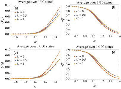
Figure 9: The inverse participation ratio $P_{2}$ [(a) and (c)] and typical multifractal dimension $\tau_{2}^{\scriptscriptstyle\mathsf{typ}}$ [(b) and (d)] in the PRBM-Hubbard model for different interaction strengths. Results are ensemble averaged over disorder realizations and portions of the spectrum, as indicated. The system size is $L=2000$ and all data are averaged over $100$ disorder realizations. The MIT is illustrated by the rising of $P_{2}$ and drop of $\tau_{2}^{\scriptscriptstyle\mathsf{typ}}$ near $\alpha=1$. Repulsive Hubbard-$U$ produces a delocalizing correction to the system, leading to smaller $P_{2}$ for stronger interaction. This is consistent with the enhanced DOS due to Altshuler-Aronov effects in the spin-triplet channel, Fig. 3.

As reviewed in Sec. II.1, the noninteracting MIT can be identified via the scaling behavior of the IPR [Eq. (2.4)] with system size. For our Hartree-Fock numerics in the spinful PRBM-Hubbard model, we define the IPR and the effective multifractal dimension $\tau_{2}$ via

$$P_{2}=\sum_{i}\left|\sum_{\sigma}\left|\psi_{i\sigma}\right|^{2}\right|^{2}\,,\quad\tau_{2}=-\ln{P_{2}}/\ln{L}.$$ (2.27)

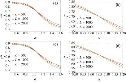
Figure 10: The typical fractal dimension $\tau_{2}^{\scriptscriptstyle\mathsf{typ}}$ for the PRBM-Hubbard model with $U=1$ and different system sizes. (a) and (b): data that is averaged over $1/5$ of the energy spectrum around Fermi energy; (c) and (d): data averaged over $1/10$ of the states around Fermi energy. The $\tau_{2}^{\scriptscriptstyle\mathsf{typ}}$ curves for different system sizes intersect at the same point, indicating that an estimate of the transition point can be extracted from finite-size scaling.

Fig. 9 shows the averaged IPR $\left\langle P_{2}\right\rangle$ and typical $\tau_{2}^{\scriptscriptstyle\mathsf{typ}}$ for different interaction strengths. The data shown in Fig. 9 are averaged over disorder realizations and states around the Fermi energy. The typical $\tau_{2}^{\scriptscriptstyle\mathsf{typ}}$ is defined as the ensemble and state average of the exponent $\tau_{2}$ (via the average of the logarithm $\left\langle\ln P_{2}\right\rangle$ rather than the log of the average $\ln\left\langle P_{2}\right\rangle$). The spectrum-wide Anderson transition approximately survives in the presence of the interactions. The wave functions receive antilocalizing corrections from the interactions (consistent with magnetic fluctuations and the enhanced DOS), which is shown by the smaller $P_{2}$ (correspondingly, larger $\tau_{2}^{\scriptscriptstyle\mathsf{typ}}$) for the interacting system compared to the non-interacting one.

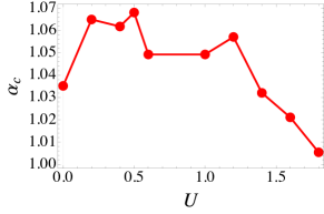
Figure 11: The interacting Anderson-Mott transition point $\alpha_{c}$ in the PRBM-Hubbard model. The transition point $\alpha_{c}$ is obtained as the crossing point of the typical multifractal dimension $\tau_{2}^{\scriptscriptstyle\mathsf{typ}}$ of $L=2000$ and $L=500$. The $L=2000$ and $L=500$ systems are averaged over $100$ and $400$ disorder realizations, respectively. Weak repulsive interaction results in anti-localizing correction to the Anderson transition and increases $\alpha_{c}$, while Mott localization starts to play a role for strong interactions.

Fig. 10 shows the system-size scaling of the typical multifractal dimension $\tau_{2}^{\scriptscriptstyle\mathsf{typ}}$. The $\tau_{2}^{\scriptscriptstyle\mathsf{typ}}$ at different system sizes intersect at the same point; the latter estimates location of the interaction-dressed MIT. The estimated critical point of the interacting Anderson-Mott transition is shown in Fig. 11. Near the critical point, the spin-triplet interaction dominates and moderate bare interaction strengths produce an anti-localizing correction to the single-particle wave functions, driving the transition point to larger $\alpha$. When the interaction is strong, Mott physics steps in and results in localizing correction due to the correlation effects.

III Technical details for mean-field numerics

We employ the self-consistent Hartree-Fock approximation to solve the PRBM-Hubbard model in Eq (2.1),

$$Un_{i\uparrow}n_{i\downarrow}= \,Un_{i\uparrow}\langle n_{i\downarrow}\rangle+U\langle n_{i\uparrow}\rangle n_{i\downarrow}-U\langle n_{i\uparrow}\rangle\langle n_{i\downarrow}\rangle$$

$$\,-U\langle c_{i\uparrow}^{\dagger}c_{i\downarrow}\rangle c_{i\downarrow}^{\dagger}c_{i\uparrow}-Uc_{i\uparrow}^{\dagger}c_{i\downarrow}\langle c_{i\downarrow}^{\dagger}c_{i\uparrow}\rangle$$

$$\,+U\langle c_{i\uparrow}^{\dagger}c_{i\downarrow}\rangle\langle c_{i\downarrow}^{\dagger}c_{i\uparrow}\rangle\,.$$ (3.1)

The first line gives the local Hartree shift and the second line corresponds to the Fock terms. By a priori choosing the $z$-axis as the possible symmetry-breaking direction of spin polarization, we can ignore the Fock terms and the Hartree-Fock and Hartree approximations are equivalent [64]. Thus, we set the initial value of the Fock terms to $0$ and they are not generated in self-consistent mean-field theory. Then we numerically solve the mean-field Hamiltonian self-consistently (including the inhomogeneous Hartree shifts) and ensemble average over disorder realizations to obtain the physical quantities.

In the self-consistent Hartree-Fock numerics, the local density of spin up and down electrons are evaluated iteratively according to the mean-field equation in Eq. (3.1). The difference of ${n_{i\sigma}}$ between two subsequent iterations are defined as,

$$\Delta n=\frac{1}{L}\sqrt{\sum_{i\sigma}\left(n_{i\sigma}^{m+1}-n_{i\sigma}^{m}\right)^{2}}\,.$$ (3.2)

Here $n_{i\sigma}^{m}$ is the density of spin $\sigma$ electrons at site $i$ in the $m$-th iteration. We use $\Delta n<10^{-6}$ as the criteria for the convergence of the self-consistent mean-field theory.

In disordered systems, it is known that the straightforward iteration procedure in Eq. (3.1) suffers from convergence issues [65]. The iterations can get stuck and oscillate between metastable states at the local extrema of the mean-field functional. The oscillation is especially serious and the convergence condition is very hard to be reached with finite iterations for generic initial conditions in the Anderson insulating phase, where single-particle wave functions are strongly localized. In our numerics, we employ Broyden’s method [66, 67] to accelerate and ensure the convergence of the iterative numerics. The iterations converge well even deep in the localized phase when the method is applied.

IV Keldysh response theory

IV.1 Non-linear sigma model

The NLsM for the non-interacting PRBM was first studied in Ref. [41]. In Keldysh field theory [43, 44], the action can be written as

$$S_{0}=\frac{1}{2\lambda}\intop_{k}\mathsf{Tr}\left[|k|^{\sigma}\,\hat{Q}(k)\,\hat{Q}(k)\right]+ih\intop_{x}\mathsf{Tr}\left[\hat{\omega}\,\hat{Q}(x)\right].$$ (4.1)

Here the exponent $\sigma=2\alpha-1$, and $h=\pi\nu_{0}$ characterizes the DOS at the Fermi energy. The coupling $\lambda$ is the inverse of the superdiffusive “conductivity” [Eq. (2.13)]. For the unitary class studied here, the matrix field $\hat{Q}(x)\rightarrow Q_{\omega,\omega^{\prime}}^{s\tau,s^{\prime}\tau^{\prime}}\sim c_{s,\tau}(\omega,x)\bar{c}_{s^{\prime},\tau^{\prime}}(\omega^{\prime},x)$ describes hydrodynamic diffuson modes of the disordered system, and carries indices in frequency ($\omega,\omega^{\prime}$) $\otimes$ spin ($s,s^{\prime}$) $\otimes$ Keldysh ($\tau,\tau^{\prime}$) spaces. $\hat{Q}(k)$ denotes the Fourier transform of the position-space field $\hat{Q}(x)$. The latter satisfies everywhere the local constraint $\hat{Q}^{2}(x)=\hat{1}$. In Eq. (4.1), $\hat{\omega}$ is the diagonal matrix of frequencies that span the real line.

Compared to the NLsM describing the dirty electron gas near two dimensions, Eq. (4.1) is nonlocal due to the non-analytic kinetic term when $\sigma<2$, which arises from the long-ranged hopping in the PRBM model. For the PRBM with $a(r)$ given by Eq. (2.3) and $1/2<\alpha<3/2$, the coupling strength $\lambda$ can be evaluated as

$$\lambda=\frac{\pi J_{0}}{b^{2\alpha}c_{\alpha}}\,,\quad c_{\alpha}=\int_{0}^{\infty}dx\,x^{-2\alpha}(1-\cos{x})\,.$$ (4.2)

Here $J_{0}$ is given by Eq. (2.8), and $c_{\alpha}$ is an order-one constant. The parameter $\lambda\sim b^{1-2\alpha}$, so that the NLsM is in the weak coupling regime when $b\gg 1$. The NLsM is renormalizable at $\sigma=\alpha=1$, and exhibits a spectrum-wide Anderson MIT for this parameter value [41, 42].

A repulsive Hubbard $U>0$ gives rise to repulsive density-density (spin-singlet) $U_{s}>0$ and attractive spin-triplet interactions $U_{t}<0$ near the Fermi surface [4, 8]. These can be incorporated into the interacting version of the Keldysh NLsM. Following conventions in Ref. [45], the action reads

$$S= S_{0}+ih\intop_{x}\mathsf{Tr}\left[\left(\tilde{V}_{\mathsf{cl}}+\tilde{V}_{\mathsf{q}}\hat{\tau}^{1}\right)\hat{M}_{F}\left(\hat{\omega}\right)\hat{Q}\,\hat{M}_{F}\left(\hat{\omega}\right)\right]$$

$$-i\frac{4h}{\pi}\intop_{t,x}\tilde{V}_{\mathsf{cl}}\tilde{V}_{\mathsf{q}}-i\frac{2}{U_{s}}\intop_{t,x}\rho_{\mathsf{cl}}\rho_{\mathsf{q}}$$

$$-ih\intop_{x}\mathsf{Tr}\left[\left(\tilde{\bm{B}}_{\mathsf{cl}}+\tilde{\bm{B}}_{\mathsf{q}}\hat{\tau}^{1}\right)\cdot\hat{\bm{\mathrm{s}}}\,\hat{M}_{F}\left(\hat{\omega}\right)\hat{Q}\,\hat{M}_{F}\left(\hat{\omega}\right)\right]$$

$$-i\frac{4h}{\pi}\intop_{t,x}\tilde{B}_{\mathsf{cl}}\cdot\tilde{B}_{\mathsf{q}}-i\frac{2}{U_{t}}\intop_{t,{x}}\bm{S}_{\mathsf{cl}}\cdot\bm{S}_{\mathsf{q}}\,.$$ (4.3)

The Pauli matrices $\{\hat{\tau}^{a}\}$ act on Keldysh space, while $\{\hat{s}^{a}\}$ act on spin-1/2 components; $\hat{\bm{\mathrm{s}}}$ is the vector of spin matrices. The operator $\hat{M}_{F}$ encodes the distribution function of the electrons,

$$\hat{M}_{F}\left(\omega\right)=\left[\begin{array}[]{cc}1&F(\omega)\\ 0&-1\end{array}\right]\,,$$ (4.4)

with $F(\omega)=\tanh(\beta\omega/2)=1-2f(\omega)$; $f$ is the equilibrium Fermi-Dirac distribution. The local fields $\rho(t,x)$ and $\bm{S}(t,x)$ encode the dynamical components of the electron particle and spin densities, and the subscripts $\mathsf{cl}$ and $\mathsf{q}$ denote the classical and quantum components in Keldysh field theory. In addition, $V$ and $\bm{B}$ represent external electric and magnetic fields used to define response functions. In Eq. (4.3), we employ the notations

$$\tilde{V}_{\mathsf{cl/q}}=V_{\mathsf{cl/q}}+\rho_{\mathsf{cl/q}}\,,\qquad\tilde{\bm{B}}_{\mathsf{cl/q}}=\bm{B}_{\mathsf{cl/q}}-\bm{S}_{\mathsf{cl/q}}\,.$$ (4.5)

IV.2 Density of states

In the Keldysh NLsM, the density of states can be obtained via

$$\nu\left(\omega\right)=\frac{\nu_{0}}{2}\mathsf{Tr}\left[\hat{\tau}^{3}\hat{Q}_{\omega,\omega}(x)\right]\,$$ (4.6)

Here $\nu_{0}$ is the density of states per spin at zero energy and $\hat{\tau}^{3}$ is the Pauli matrix in Keldysh space.

Figure 12: The Feynman diagrams contributing to the Altshuler-Aronov correction to the density of states with singlet [(a) and (b)] and triplet channel [(c) and (d)] interactions.

We employ the “$\pi$-$\sigma$” parameterization of the $Q$ matrix field [45],

$$\hat{Q}\equiv\begin{bmatrix}\sqrt{\hat{1}-\hat{W}\,\hat{W}^{\dagger}}&\hat{W}\\ \hat{W}^{\dagger}&-\sqrt{\hat{1}-\hat{W}^{\dagger}\hat{W}}\end{bmatrix}_{\tau},$$ (4.7)

where $\hat{W}\rightarrow W_{\omega,\omega^{\prime}}^{s,s^{\prime}}(x)$ is an unconstrained, complex-valued matrix field with indices in frequency and spin spaces. Then

$$\tilde{\nu}\left(\omega\right)= 4-\frac{1}{2}\sum_{s_{1}s_{2}}\,\intop_{\Omega,k}\left\langle W_{\omega\Omega}^{s_{2}s_{1}}\left(k\right)W_{\Omega\omega}^{\dagger s_{1}s_{2}}\left(k\right)\right\rangle-\frac{1}{2}\sum_{s_{1}s_{2}}\,\intop_{\Omega,k}\left\langle W_{\Omega\omega}^{s_{2}s_{1}}\left(k\right)W_{\omega\Omega}^{\dagger s_{1}s_{2}}\left(k\right)\right\rangle+\mathcal{O}\left(W^{4}\right)\,.$$ (4.8)

Here $\tilde{\nu}=2\nu(\omega)/\nu_{0}$. The diagrams with bare propagators cancel because the DOS is noncritical without interactions. Non-vanishing diagrams arise due to the interactions (Altshuler-Aronov corrections [7]). At one-loop order these are shown in Fig. 12. The correction in the singlet channel in Figs. 12(a) and (b) is given by

$$\delta\tilde{\nu}_{s}=-\left(ih\right)^{2}\intop_{\Omega,k}\left[\begin{array}[]{r}\Delta_{0}^{2}\left(\Omega-\omega,k\right)i\Delta_{\rho}^{R}\left(\omega-\Omega,k\right)\left(F_{\omega}-F_{\Omega}\right)\\ +\Delta_{0}^{2}\left(\omega-\Omega,k\right)i\Delta_{\rho}^{R}\left(\Omega-\omega,k\right)\left(F_{\Omega}-F_{\omega}\right)\end{array}\right].$$ (4.9)

Here $\Delta_{\rho}^{R}(\omega,k)$ is the retarded density propagator,

$$i\Delta_{\rho}^{R}(\omega,k)=\frac{i\pi\gamma_{s}}{4h}\frac{\Delta_{u,s}(-\omega,k)}{\Delta_{0}(-\omega,k)}\,,$$ (4.10)

with

$$\Delta_{0}(\omega,k) =\frac{1}{\frac{\left|k\right|^{\sigma}}{\lambda}+i\frac{h\omega}{2}},\,$$ (4.11a)

$$\Delta_{u,s}(\omega,k) =\frac{1}{\frac{\left|k\right|^{\sigma}}{\lambda}+i\frac{h\omega}{2}(1-\gamma_{s})}\,.$$ (4.11b)

The parameter $\gamma_{s}$ is the dimensionless interaction strength in the spin-singlet channel, which incorporates the Fermi-liquid renormalization of the compressibility

$$\gamma_{s}=\frac{2U_{s}h/\pi}{1+2U_{s}h/\pi}\,.$$ (4.12)

Ignoring the irrelevant terms at order of $\omega^{2}$, we have

$$\delta\tilde{\nu}_{s}=\frac{i\pi h\gamma_{s}}{2}\intop_{\Omega,k}F_{\Omega}\,\Delta_{0}\left(-\Omega,k\right)\Delta_{u,s}\left(-\Omega,k\right)\,.$$ (4.13)

Similarly, the correction due to the triplet channel interaction is given by

$$\delta\tilde{\nu}_{t}=\frac{i\pi h\gamma_{t}}{2}\intop_{\Omega,k}F_{\Omega}\,\Delta_{0}\left(-\Omega,k\right)\Delta_{u,t}\left(-\Omega,k\right)\,.$$ (4.14)

Here we have

$$\Delta_{u,t}(\omega,k)=\frac{1}{\frac{\left|k\right|^{\sigma}}{\lambda}+i\frac{h\omega}{2}(1-\gamma_{t})}\,,$$ (4.15)

$$\gamma_{t}=\frac{2U_{t}h/\pi}{1+2U_{t}h/\pi}\,.$$ (4.16)

Define

$$I_{1}=\frac{i\pi h\gamma}{2}\intop_{\Omega,k}F_{\Omega}\,\Delta_{0}\left(-\Omega,k\right)\Delta_{u}\left(-\Omega,k\right)\,.$$ (4.17)

The integral is UV divergent when $\sigma\leq 1$. Integrating out $\Omega$ first from $-\infty$ to $+\infty$, we have

$$I_{1}=\lambda\ln\left(1-\gamma\right)\intop_{l}\frac{1}{l^{\sigma}}\,.$$ (4.18)

In the extended phase ($\sigma<1$), we obtain

$$I_{1}=\frac{\lambda\Lambda_{k}^{1-\sigma}}{\pi\left(1-\sigma\right)}\ln\left(1-\gamma\right)\,.$$ (4.19)

Here $\Lambda_{k}$ is the UV cutoff in momentum. The corresponding correction to the DOS in the ergodic phase is

$$\delta{\nu}(\omega)=\frac{\nu_{0}\lambda\Lambda_{k}^{1-\sigma}}{2\pi\left(1-\sigma\right)}\left[\ln\left(1-\gamma_{s}\right)+3\ln\left(1-\gamma_{t}\right)\right].$$ (4.20)

At the noninteracting critical point $\sigma=1$, we have

$$I_{1}=\frac{\lambda}{\pi}\ln\left(1-\gamma\right)\ln\left(\frac{\Lambda}{T}\right)\,,$$ (4.21)

which leads to the DOS correction in Eq. (2.9).

We can also calculate the perturbative interaction correction in the localized phase. The integral $I_{1}$ is UV and IR convergent and we cannot simply extract the UV behavior of $\Omega$ first. We have

$$I_{1}= -\frac{\lambda\left(2-\gamma\right)\gamma D^{1-\frac{1}{\sigma}}T^{\frac{1}{\sigma}-1}}{4\pi\sigma}\int_{0}^{\infty}dx\int_{-\infty}^{\infty}dy\frac{x^{\frac{1}{\sigma}}y\tanh\frac{y}{2}}{\left(x^{2}+y^{2}\right)\left[x^{2}+\left(1-\gamma\right)^{2}y^{2}\right]}\,.$$ (4.22)

The overall correction to the DOS in the localized phase diverges as a power-law with decreasing temperature,

$$\delta\tilde{\nu}\left(\omega\right)=-\lambda D^{1-\frac{1}{\sigma}}T^{\frac{1}{\sigma}-1}\left[\mathfrak{a}_{s}\mathfrak{A}_{s}+3\mathfrak{a}_{t}\mathfrak{A}_{t}\right]$$ (4.23)

Here $\mathfrak{a}_{s/t}$ are defined via

$$\mathfrak{a}_{s/t}=(2-\gamma_{s/t})\gamma_{s/t}\,,$$ (4.24)

and

$$\,\mathfrak{A}_{s/t}$$

$$\,\,=\frac{1}{4\pi\sigma}\int_{0}^{\infty}dx\int_{-\infty}^{\infty}dy\frac{x^{\frac{1}{\sigma}}y\tanh\frac{y}{2}}{\left(x^{2}+y^{2}\right)\left[x^{2}+\left(1-\gamma_{s/t}\right)^{2}y^{2}\right]}\,.$$ (4.25)

We have introduced the dimensionless coordinates $x=\frac{D\left|k\right|^{\sigma}}{T}$ and $y=\frac{\Omega}{T}$.

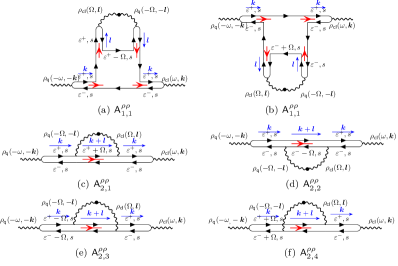
Figure 13: Diagrams $\mathsf{A}^{\rho\rho}$ contributing to the Altshuler-Aronov correction to the density response function in the spin-singlet interaction channel.

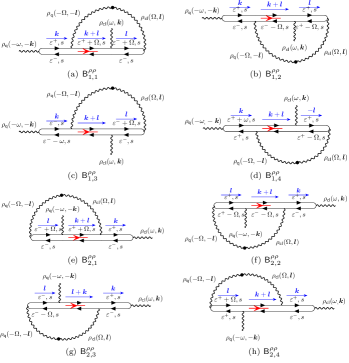
Figure 14: “Wave function renormalization” diagrams $\mathsf{B}^{\rho\rho}$ contributing to the Altshuler-Aronov correction to the density response function in the spin-singlet interaction channel.

IV.3 Density response

The retarded self-energy for the dynamical density field $\rho(t,x)$ due to singlet-channel interactions can be obtained as

$$-i\Sigma_{\rho}^{R}=-\frac{h^{2}}{2}\Delta_{0}^{2}\left(-\omega,k\right)\intop_{\varepsilon}\left(F_{\varepsilon^{-}}-F_{\varepsilon^{+}}\right)\left[\Sigma_{X}^{\mathsf{A}^{\rho\rho}}+\Sigma_{X}^{\mathsf{B}^{\rho\rho}}\right]\,,$$ (4.26)

Here $\varepsilon_{\pm}=\varepsilon\pm\omega/2$ and the $\mathsf{A}^{\rho\rho}$ and $\mathsf{B}^{\rho\rho}$ diagrams are shown in Figs. 13 and 14, respectively. In the theory of the 2D dirty electron gas, the $\mathsf{A}$ diagrams in Fig. 13 give the direct correction to the conductivity and the $\mathsf{B}$ diagrams in Fig. 14 determine the wave function renormalization of the $Q$ field; both are Altshuler-Aronov corrections in the unitary class. In the NLsM for the PRBM-Hubbard model, the kinetic term is nonlocal and has fractional dependence on the momentum. As a result, the $\mathsf{A}$ diagrams do not yield a term proportional to $|k|^{\sigma}$ and the correction to the superdiffusion constant comes only from the wave function renormalization in Fig. 14. The $\mathsf{A}$ diagrams give a term proportional to frequency that is necessary to satisfy the Ward identity for charge conservation.

We obtain

$$\Sigma_{X}^{\rho}= \,\frac{i\pi h\gamma_{s}\left|k\right|^{\sigma}}{2\lambda}$$

$$\,\times\intop_{\Omega,l}\Delta_{0}\left(-\Omega,l\right)\Delta_{u,s}\left(-\Omega,l\right)\left(F_{\varepsilon+\Omega}-F_{\varepsilon-\Omega}\right).$$ (4.27)

Here $\Sigma_{X}^{\rho}=\Sigma_{X}^{A^{\rho\rho}}+\Sigma_{X}^{B^{\rho\rho}}$ and we discard the higher-order terms in $\omega$ and the term $F_{\varepsilon}^{+}-F_{\varepsilon}^{-}$, which vanishes after integrating out $\Omega$ and $l$. In this model, the Ward identity requires that the superdiffusive relation $\omega\sim c\left|k\right|^{\sigma}$ is unaltered by the interaction and disorder scattering. As a result $\Sigma_{X}$ must be proportional to $\left|k\right|^{\sigma}$, which is exactly what we have obtained in Eq. (4.27). The correction to the density response function in the extended phase and at critical point can be obtained by using the integral in Eq. (4.17) and the identity $\intop_{\varepsilon}\left(F_{\varepsilon^{-}}-F_{\varepsilon^{+}}\right)=-\frac{\omega}{\pi}\,.$ In the extended phase ($\sigma<1$), the correction to the density response function is

$$\delta\Pi\left(\omega,k\right)= \frac{i\left(1-\gamma_{s}\right)^{2}h^{2}\omega\left|k\right|^{\sigma}\Lambda_{k}^{1-\sigma}}{2\pi^{2}\left(1-\sigma\right)}$$

$$\times\Delta_{u,s}^{2}\left(-\omega,k\right)\ln\left(1-\gamma_{s}\right)\,.$$ (4.28)

The quantum correction to the superdiffusive “conductivity” [Eq. (2.13)] in the extended phase $\sigma<1$ is then given by,

$$\delta\mathfrak{g} =\frac{2\Lambda_{k}^{1-\sigma}}{\pi^{2}\left(1-\sigma\right)}\ln\left(1-\gamma_{s}\right).$$ (4.29)

At the critical point ($\sigma=1$),

$$\delta\mathfrak{g}=\frac{2}{\pi^{2}}\ln\left(1-\gamma_{s}\right)\ln\left(\frac{\Lambda}{T}\right)\,.$$ (4.30)

Here $\Lambda$ is the UV cutoff in energy and it is related to the momentum cutoff via the superdiffusive relation $\Lambda={D}\Lambda_{k}$.

On the localized side $\sigma>1$, the integral for the Altshuler-Aronov correction has no UV or IR divergence and we have

$$\delta\Pi\left(\omega,k\right)= -i\frac{\lambda h^{3}\left(2-\gamma_{s}\right)\gamma_{s}\left(1-\gamma_{s}\right)^{2}D^{2-\frac{1}{\sigma}}T^{\frac{1}{\sigma}}}{8\pi^{2}\sigma}\left|k\right|^{\sigma}\Delta_{u,s}^{2}\left(-\omega,k\right)\mathfrak{B}_{s}\left(\frac{\omega}{T}\right)\,.$$ (4.31)

Here $\mathfrak{B}_{s}\left(\frac{\omega}{T}\right)$ is defined as

$$\mathfrak{B}_{s}\left(\frac{\omega}{T}\right)=4\int_{0}^{\infty}dx\int_{0}^{\infty}dy\frac{x^{\frac{1}{\sigma}}y\left[4\frac{\omega}{T}\sinh y-4y\sinh\left(\frac{\omega}{T}\right)\right]}{\left(x^{2}+y^{2}\right)\left[x^{2}+\left(1-\gamma_{s}\right)^{2}y^{2}\right]\left[\cosh\left(y\right)-\cosh\left(\frac{\omega}{T}\right)\right]}\,.$$ (4.32)

At the leading order in $\omega/T$, we have

$$\mathfrak{B}_{s}\left(\frac{\omega}{T}\right)=\mathfrak{B}_{0}\left(\gamma_{s}\right)\frac{\omega}{T}+\mathcal{O}\left(\left[\frac{\omega}{T}\right]^{3}\right)\,,$$ (4.33)

with

$$\mathfrak{B}_{0}\left(\gamma_{s}\right)=2\int_{0}^{\infty}dx\int_{0}^{\infty}dy\frac{x^{\frac{1}{\sigma}}y\left(\sinh y-y\right)}{\left(x^{2}+y^{2}\right)\left[x^{2}+\left(1-\gamma_{s}\right)^{2}y^{2}\right]\sinh^{2}\frac{y}{2}}\,.$$ (4.34)

Thus, the correction to the density response function is

$$\delta\Pi\left(\omega,k\right)=-i\frac{\lambda h^{3}\left(2-\gamma_{s}\right)\gamma_{s}\left(1-\gamma_{s}\right)^{2}D^{2-\frac{1}{\sigma}}T^{\frac{1}{\sigma}-1}\omega}{8\pi^{2}\sigma}\left|k\right|^{\sigma}\Delta_{u,s}^{2}\left(-\omega,k\right)\mathfrak{B}_{0}\left(\gamma_{s}\right)\,.$$ (4.35)

The quantum correction to the superdiffusive “conductivity” is given by

$$\delta\mathfrak{g}=-\frac{\lambda h\mathfrak{a}_{s}D^{2-\frac{1}{\sigma}}T^{\frac{1}{\sigma}-1}}{2\pi^{2}\sigma}\mathfrak{B}_{0}\left(\gamma_{s}\right)\,.$$ (4.36)

The quantum correction diverges as $T\to 0$ with power-law $T^{\frac{1}{\sigma}-1}$ in the localized side ($\sigma>1$), and it decreases the superdiffusive “conductivity” as $\gamma_{s}>0$ and $\mathfrak{B}_{0}\left(\gamma_{s}\right)>0$. Therefore, the singlet channel interactions result in localizing corrections. This is similar to the situation of the 2D electron gas [9, 10, 4].

For the interactions in the spin-triplet channel, the correction to the density response is given by diagrams similar to those in Figs. 13 and 14. The total correction to $\delta\mathfrak{g}$ in the ergodic phase ($\sigma<1$) and at the noninteracting critical point ($\sigma=1$) is given by Eqs. (2.14) and (2.15), respectively. In the localized phase with $\sigma>1$,

$$\delta\mathfrak{g}\left(\omega\right)=-\frac{3\lambda h\mathfrak{a}_{t}D^{2-\frac{1}{\sigma}}T^{\frac{1}{\sigma}-1}}{2\pi^{2}\sigma}\mathfrak{B}_{0}\left(\gamma_{t}\right)\,.$$ (4.37)

The natural sign of the spin triplet interaction $\gamma_{t}$ is negative for repulsive interactions [4, 8]. Thus, the quantum effect in the spin-triplet channel results in an anti-localizing correction to transport.

IV.4 Spin susceptibility

The spin response function $\chi_{ij}\left(\omega,k\right)$ encodes both spin transport and the static spin susceptibility. Spin and charge transport are renormalized the same way in the absence of magnetic order. Different from the charge compressibility that receives no quantum corrections [4], quantum interference effects can enhance or suppress the static spin susceptibility. The latter is determined by the $\omega\to 0$ limit of $\chi_{ij}\left(\omega,k\right)$. There are two groups of diagrams $\mathsf{C},\mathsf{D}$ contributing to the static magnetic response function shown in Fig. 15.

Up to irrelevant corrections, the self-energy for the dynamical spin field $\bm{S}(t,x)$ is

$$-i\Sigma_{\mathsf{sp}}^{R,\mathsf{C}}=$$

$$2i\pi \,h^{3}\gamma_{t}\delta_{ij}\intop_{\Omega l}\Delta_{0}^{2}\left(-\Omega,l\right)\Delta_{u,t}\left(-\Omega,l\right)\left(B_{\Omega}-B_{0}\right)\,.$$ (4.38)

Here we have used the identity $B_{\omega}\equiv\intop_{\varepsilon}\left(1-F_{\varepsilon}F_{\varepsilon+\omega}\right)=\frac{\omega}{\pi}\coth\left(\frac{\omega}{2T}\right)\,.$ Discarding higher-order terms in $\omega$ and $k$, we have

$$-i\Sigma_{\mathsf{sp}}^{R,\mathsf{D}}= -2h^{6}\delta_{ij}\intop_{\varepsilon_{1}\varepsilon_{2}\Omega l}\Delta_{0}^{4}\left(-\Omega,l\right)\left[i\Delta_{\mathsf{sp}}^{R}\left(\Omega,l\right)\right]^{2}\left\{\begin{array}[]{r}2\left(F_{\varepsilon_{1}^{+}+\Omega}-F_{\varepsilon_{1}^{+}}\right)\left(F_{\varepsilon_{2}^{-}+\Omega}-F_{\varepsilon_{2}^{+}}\right)F_{\varepsilon_{1}^{-}+\Omega}\\ -2\left(F_{\varepsilon_{1}^{-}+\Omega}-F_{\varepsilon_{1}^{-}}\right)\left(F_{\varepsilon_{2}^{-}+\Omega}-F_{\varepsilon_{2}^{+}}\right)F_{\varepsilon_{1}^{+}}\end{array}\right\}\,.$$ (4.41)

Integrating out $\varepsilon_{1}$ and $\varepsilon_{2}$ gives

$$-i\Sigma_{\mathsf{s}}^{R,\mathsf{D}}=\frac{\pi^{2}h^{4}\gamma_{t}^{2}\delta_{ij}}{2}\intop_{\Omega l}\Delta_{0}^{2}\left(-\Omega,l\right)\Delta_{u,t}^{2}\left(-\Omega,l\right)\frac{\Omega}{\pi}\left(B_{\Omega}-B_{0}\right)+\mathcal{O}\left(\omega\right)\,.$$ (4.42)

In the ergodic phase ($\sigma<1$), the integrals in Eq. (4.38) and (4.42) are UV divergent and IR convergent. We can first integrate out $\Omega$ from $-\infty$ to $+\infty$ and obtain,

$$-i\Sigma_{\mathsf{sp}}^{R,\mathsf{C}} =\frac{16i}{\pi}\delta_{ij}\left[1+\frac{1}{\gamma_{t}}\ln\left(1-\gamma_{t}\right)\right]\intop_{l}\frac{1}{{D}\left|l\right|^{\sigma}}\,,$$ (4.43)

$$-i\Sigma_{\mathsf{sp}}^{R,\mathsf{D}} =8\gamma_{t}^{2}\delta_{ij}\intop_{l}\frac{1}{\pi\gamma_{t}^{2}i{D}\left|l\right|^{\sigma}}\left[1+\frac{1}{1-\gamma_{t}}+\frac{2}{\gamma_{t}}\ln\left(1-\gamma_{t}\right)\right]\,.$$ (4.44)

Here we use the integrals

$$\intop_{\Omega}\frac{B_{\Omega}-B_{0}}{\left[i{D}\left|l\right|^{\sigma}+\Omega\right]^{2}\left[i{D}\left|l\right|^{\sigma}+\Omega\left(1-\gamma_{t}\right)\right]} \approx-\frac{1}{\pi^{2}\gamma_{t}}\left[1+\frac{1}{\gamma_{t}}\ln\left(1-\gamma_{t}\right)\right]\frac{i}{{D}\left|l\right|^{\sigma}}\,,$$ (4.45a)

$$\intop_{\Omega}\frac{\Omega\left(B_{\Omega}-B_{0}\right)}{\left[i{D}\left|l\right|^{\sigma}+\Omega\right]^{2}\left[i{D}\left|l\right|^{\sigma}+\Omega\left(1-\gamma_{t}\right)\right]^{2}} \approx\frac{1}{\pi^{2}\gamma_{t}^{2}}\left[1+\frac{1}{1-\gamma_{t}}+\frac{2}{\gamma_{t}}\ln\left(1-\gamma_{t}\right)\right]\frac{1}{i{D}\left|l\right|^{\sigma}}\,.$$ (4.45b)

Thus we have

$$-i\Sigma_{\mathsf{sp}}^{R,\mathsf{CD}}=-i\Sigma_{\mathsf{sp}}^{R,\mathsf{C}}-i\Sigma_{\mathsf{sp}}^{R,\mathsf{D}}=-\frac{i4\lambda h\delta_{ij}}{\pi}\frac{\gamma_{t}}{1-\gamma_{t}}\intop_{l}\frac{1}{\left|l\right|^{\sigma}}\,.$$ (4.46)

Integrating out $l$ yields

$$-i\Sigma_{\sigma}^{R,\mathsf{CD}}=-\frac{i4\lambda h\delta_{ij}}{\pi^{2}\left(1-\sigma\right)}\frac{\gamma_{t}}{1-\gamma_{t}}\Lambda_{k}^{1-\sigma}\,.$$ (4.47)

The corresponding correction to the spin density response function is

$$\delta\chi_{ij}^{\mathsf{CD}} \left(\omega,k\right)$$

$$= -\frac{2}{U_{t}^{2}}\Delta_{\mathsf{\sigma}}^{R,ii}\left(\omega,k\right)\Sigma_{\sigma}^{R,ij}\left(\omega,k\right)\Delta_{\sigma}^{R,jj}\left(\omega,k\right)$$

$$= -\frac{2\lambda h\delta_{ij}\left(1-\gamma_{t}\right)}{\pi^{2}\left(1-\sigma\right)}\frac{\left(\frac{\left|k\right|^{\sigma}}{\lambda}-\frac{ih\omega}{2}\right)^{2}}{\left[\frac{\left|k\right|^{\sigma}}{\lambda}-\frac{ih\omega}{2}\left(1-\gamma_{t}\right)\right]^{2}}\gamma_{t}\Lambda_{k}^{1-\sigma}\,.$$ (4.48)

Here $U_{t}=\frac{\pi}{2h}\frac{\gamma_{t}}{1-\gamma_{t}}$. In the static limit, $\omega\to 0$, we have

$$\delta\chi_{ij}\left(\omega\to 0\right)=\frac{2\lambda h\delta_{ij}\left(1-\gamma_{t}\right)}{\pi^{2}\left(1-\sigma\right)}\gamma_{t}\Lambda_{k}^{1-\sigma}\,.$$ (4.49)

Recall that the bare (semiclassical) spin response function is given by Eq. (2.16) with $\chi_{0}=\frac{2h}{\pi}\left(1-\gamma_{t}\right)$. Then we obtain Eq. (2.18). At the noninteracting critical point there is a logarithmic divergence that can be cut in the infrared by the temperature $T$. This leads to Eq. (2.19). The latter is identical to the correction for the dirty 2D electron gas except for the numerical prefactor [9].

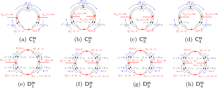
Figure 15: Diagrams $\mathsf{C}$ and $\mathsf{D}$ contributing to the static spin response function.

Now we turn to the localized phase with $\sigma>1$. In this case, the integrals are convergent in both the UV and IR limits, and we can discard the UV cutoffs $\Lambda$ and $\Lambda_{k}$. The $\mathsf{C}$ diagrams are given by

$$-i\Sigma_{\mathsf{sp}}^{R,\mathsf{C}} =2i\pi h^{3}\gamma_{t}\delta_{ij}I_{2}\,,$$ (4.50)

with

$$I_{2} =\frac{1}{4\pi^{2}}\left(\frac{2}{h}\right)^{3}\int_{-\infty}^{\infty}d\Omega\int_{-\infty}^{\infty}dl\frac{1}{\left(D\left|l\right|^{\sigma}-i\Omega\right)^{2}\left[D\left|l\right|^{\sigma}-i\Omega\left(1-\gamma_{t}\right)\right]}\left(B_{\Omega}-B_{0}\right)$$

$$=T^{\frac{1}{\sigma}-1}\frac{1}{\sigma}\left(\frac{1}{D}\right)^{\frac{1}{\sigma}}\frac{1}{2\pi^{3}}\left(\frac{2}{h}\right)^{3}\int_{-\infty}^{\infty}dy\int_{0}^{\infty}dx\frac{x^{\frac{1}{\sigma}-1}\left(y\coth\frac{y}{2}-2\right)}{\left(x-iy\right)^{2}\left[x-iy\left(1-\gamma_{t}\right)\right]}\,.$$ (4.51)

The $\mathsf{D}$ diagrams are given by

$$-i\Sigma_{\mathsf{sp}}^{R,\mathsf{D}} =\frac{\pi^{2}h^{4}\gamma_{t}^{2}\delta_{ij}}{2}I_{3}\,,$$ (4.52)

with

$$I_{3} =\frac{1}{4\pi^{3}}\left(\frac{2}{h}\right)^{4}\int_{-\infty}^{\infty}dl\int_{-\infty}^{\infty}d\Omega\frac{\Omega\left(B_{\Omega}-B_{0}\right)}{\left(D\left|l\right|^{\sigma}-i\Omega\right)^{2}\left[D\left|l\right|^{\sigma}-i\Omega\left(1-\gamma_{t}\right)\right]^{2}}$$

$$=T^{\frac{1}{\sigma}-1}\frac{1}{\sigma}\left(\frac{1}{D}\right)^{\frac{1}{\sigma}}\frac{1}{2\pi^{4}}\left(\frac{2}{h}\right)^{4}\int_{0}^{\infty}dx\int_{-\infty}^{\infty}dy\frac{x^{\frac{1}{\sigma}-1}y\left(y\coth\frac{y}{2}-2\right)}{\left(x-iy\right)^{2}\left[x-iy\left(1-\gamma_{t}\right)\right]^{2}}\,.$$ (4.53)

Thus

$$-i\Sigma_{\mathsf{sp}}^{R,\mathsf{CD}}=-\frac{8i\delta_{ij}}{\pi^{2}}T^{\frac{1}{\sigma}-1}\frac{1}{\sigma}\left(\frac{1}{D}\right)^{\frac{1}{\sigma}}\left[\mathfrak{I}_{1}\gamma_{t}+\mathfrak{I}_{2}\gamma_{t}^{2}\right]\,.$$ (4.54)

Here

$$\mathfrak{I}_{1} =-\int_{0}^{\infty}dx\int_{-\infty}^{\infty}dy\frac{x^{\frac{1}{\sigma}}\left[x^{2}-\left(3-2\gamma_{t}\right)y^{2}\right]\left(y\coth\frac{y}{2}-2\right)}{\left(x^{2}+y^{2}\right)^{2}\left[x^{2}+y^{2}\left(1-\gamma_{t}\right)^{2}\right]}\,,$$ (4.55a)

$$\mathfrak{I}_{2} =-\int_{0}^{\infty}dx\int_{-\infty}^{\infty}dy\frac{x^{\frac{1}{\sigma}}y^{2}\left(2-\gamma_{t}\right)\left[x^{2}-y^{2}\left(1-\gamma_{t}\right)\right]\left(y\coth\frac{y}{2}-2\right)}{\left(x^{2}+y^{2}\right)^{2}\left[x^{2}+y^{2}\left(1-\gamma_{t}\right)^{2}\right]^{2}}\,.$$ (4.55b)

The correction to the spin response function is obtained as,

$$\delta\chi_{ij}^{\mathsf{CD}}\left(\omega,k\right)=-\frac{2\delta_{ij}T^{\frac{1}{\sigma}-1}\left(1-\gamma_{t}\right)^{2}}{\pi^{2}\sigma D^{\frac{1}{\sigma}}}\left(\frac{\frac{\left|k\right|^{\sigma}}{\lambda}-\frac{ih\omega}{2}}{\frac{\left|k\right|^{\sigma}}{\lambda}-\frac{ih\omega}{2}\left(1-\gamma_{t}\right)}\right)^{2}\left(\mathfrak{I}_{1}\gamma_{t}+\mathfrak{I}_{2}\gamma_{t}^{2}\right)\,.$$ (4.56)

In the static limit ($\omega\to 0)$, we have

$$\delta\chi_{ij}=-\frac{2\delta_{ij}T^{\frac{1}{\sigma}-1}\left(1-\gamma_{t}\right)^{2}}{\pi^{2}\sigma D^{\frac{1}{\sigma}}}\left(\mathfrak{I}_{1}\gamma_{t}+\mathfrak{I}_{2}\gamma_{t}^{2}\right)\,.$$ (4.57)

Thus, we obtain the static spin susceptibility in terms of the non-interacting one,

$$\chi_{ij}=\delta_{ij}\chi_{0}\left[1-\frac{2T^{\frac{1}{\sigma}-1}\left(1-\gamma_{t}\right)}{\pi\sigma D^{\frac{1}{\sigma}}h}\gamma_{t}\left(\mathfrak{I}_{1}+\mathfrak{I}_{2}\gamma_{t}\right)\right]\,.$$ (4.58)

Fig. 16 shows $\mathfrak{I}_{1}+\mathfrak{I}_{2}\,\gamma_{t}$ as a function of the spin-triplet interaction strength $\gamma_{t}$ (red line). It is always positive for attractive $\gamma_{t}<0$, and the static spin susceptibility in the localized phase is therefore enhanced compared to its bare value. The blue dashed line in Fig. 16 shows the coefficient $\left(\mathfrak{I}_{1}+\mathfrak{I}_{2}\gamma_{t}\right)(1-\gamma_{t})$, which is almost a constant over the range plotted. At low temperature, the correction to the spin susceptibility diverges in a power-law fashion $\sim T^{1/\sigma-1}$.

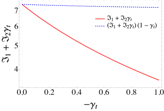
Figure 16: The dependence of the coefficients for the quantum correction to the magnetic susceptibility in the localized phase as a function of the spin-triplet interaction strength $\gamma_{t}$, see Eq. (4.58).

IV.5 RG-improved DOS

The interaction correction to the DOS obtained above in Sec. IV.2 treats the coupling $\lambda$, interactions $\gamma_{s/t}$ and the bare density of states as constant parameters. To more accurately account for the interaction corrections, we should turn to the RG equations, where these quantities are running parameters. The RG equations for the coupling $\lambda$, the DOS $\nu$ and the spin susceptibility can be extracted from Eqs. (2.15),  (2.9) and  (2.19), respectively. At the critical point, the RG flow equations are

$$\frac{d\lambda}{dl} =-\frac{\lambda^{2}}{2\pi}\left[\ln\left(1-\gamma_{s}\right)+3\ln\left(1-\gamma_{t}\right)\right]\,,$$ (4.59a)

$$\frac{d\ln\nu}{dl} =\frac{\lambda}{4\pi}\left[\ln\left(1-\gamma_{s}\right)+3\ln\left(1-\gamma_{t}\right)\right]\,,$$ (4.59b)

$$\frac{d\chi_{t}}{dl} =-\frac{\chi_{t}\lambda\gamma_{t}}{\pi}\,.$$ (4.59c)

The RG equation for $h$ takes the similar form as that in 2D unitary class with SU(2) symmetry,

$$\frac{d\ln h}{dl}=-\frac{\lambda}{4\pi}\left(\gamma_{s}+3\gamma_{t}\right)\,.$$ (4.60)

Thus, we obtain the RG equations for the interactions and the energy (dynamical critical scaling)

$$\frac{d\gamma_{s}}{dl} =-\frac{\lambda}{4\pi}\left(1-\gamma_{s}\right)\left(\gamma_{s}+3\gamma_{t}\right),$$ (4.61a)

$$\frac{d\gamma_{t}}{dl} =\frac{\lambda}{4\pi}\left(1-\gamma_{t}\right)\left(\gamma_{t}-\gamma_{s}\right),$$ (4.61b)

$$\frac{d\ln\varepsilon}{dl} =-d-\frac{d\ln h}{dl}=-1+\frac{\lambda}{4\pi}\left(\gamma_{s}+3\gamma_{t}\right)\,.$$ (4.61c)

The RG coupled equations in general cannot be solved exactly. However, the flow of the parameter $\lambda$ is logarithmically slow in the perturbative regime, and can therefore be initially neglected. Linearizing the flow equations for the interactions to linear order in $\gamma_{s,t}$ reveals a single relevant direction, wherein the triplet interaction $\gamma_{t}\rightarrow-\infty$, indicating the onset of strong magnetic fluctuations near the MIT. We therefore specialize to the following simplified flow equations governing the intermediate-scale flow of the DOS,

$$\frac{d\ln{\nu}}{dl} =3\lambda\ln{\left(1-\gamma_{t}\right)}\,,$$ (4.62a)

$$\frac{d\gamma_{t}}{dl} =\lambda\gamma_{t}\,,$$ (4.62b)

$$\frac{d\ln\varepsilon}{dl} =-1\,.$$ (4.62c)

Here we rescale the coupling $\lambda\to 4\pi\lambda$. We also ignore the spin-singlet interaction $\gamma_{s}$ and focus on the spin-triplet interaction $\gamma_{t}$, which dominates near the MIT. Solving the simplified RG equations, we obtain

$$\gamma_{t}(l) =\gamma_{t}(0)\,e^{\lambda l}\,,$$ (4.63)

$$\ln\left[{\frac{\nu(l)}{\nu(0)}}\right] =-3\left[\mathsf{Li}_{2}(\gamma_{t}^{0}e^{\lambda l})-\mathsf{Li}_{2}(\gamma_{t}^{0})\right]\,,$$ (4.64)

$$\ln\left[{\frac{\varepsilon(l)}{\varepsilon(0)}}\right] =-l\,.$$ (4.65)

Here $\mathsf{Li}_{2}$ is the dilogarithm function and $\gamma_{t}^{0}=\gamma_{t}(l=0)$. Identifying $\nu(l)=\nu(\varepsilon)$ and $\varepsilon(l)=\varepsilon$, we obtain Eq. (2.10). The RG-improved expression for the DOS diverges at zero energy, which is qualitatively consistent with the numerical results shown in Fig. 3.

V Conclusion

We have already summarized our main results and conclusions in the Introduction and in Secs. II.2 and II.3. We close with open questions. We have obtained good qualitative agreement between analytics and numerics in the metallic phase, indicative of a magnetic instability that occurs near the MIT. The identification of spin-glass order in the insulator was obtained numerically. Does this result survive the incorporation of correlation effects for the PRBM-Hubbard model? A natural alternative would be spin-liquid behavior, which arises in quantum spin-glass models such as the Sachdev-Ye and Sachdev-Ye-Kitaev models [68].

Another question concerns the nature of the spin glass. What are the statistics of the self-consistently determined magnetic exchange constants, and does the resulting effective spin model exhibit continuous replica symmetry breaking? It would also be interesting to consider magnonic fluctuations on top of the frozen background, incorporating magnon-magnon scattering in the insulator.

The results employed here suggest that interaction-mediated interference effects and local-moment formation and frustration are two sides of the same coin that merge continuously at the MIT. Is it possible to capture the onset of spin-glass order within the interacting sigma model formalism employed here, by allowing for replica-symmetry-broken saddle-points? Replica symmetry breaking has appeared before in sigma model calculations, but only as a formal device to recover random matrix correlations in the zero-dimensional ($\alpha=0$), non-interacting version of the PRBM model studied here [51].

  

Appendix A Spin configurations in the self-consistent numerics

Fig. 17 shows converged spin configurations of the PRBM-Hubbard model obtained by self-consistent Hartree-Fock numerics. In the extended phase ($\alpha\lesssim 1$), the local spin density is almost $0$ and there are no magnetic moments. Near the MIT ($\alpha\approx 1$), dilute magnetic moments start to form, and the density of local moments increases with $\alpha$ in the localized phase ($\alpha\gtrsim 1$). The spin polarization of the local moments is not ferromagnetic correlated, and the net magnetization is much smaller than the density of local moments, indicating the absence of ferromagnetic ordering. Fig. 18 shows the local density of spins for $\alpha=1.1$ with different initial conditions for the self-consistent calculations. The positions of the local moments are almost independent of the initial conditions. However, the sign of the local spin density is extremely sensitive to the initial conditions. The converged solutions of the PRBM-Hubbard model in the interacting, localized phase consist of a large number of nearly-degenerate states and we obtain one of them in each run of the self-consistent numerics. Each state obtained with different initial conditions can be identified as one “replica,” and the initial condition-dependence of the ground states implies the replica symmetry breaking in the system, as discussed in Sec. II.3.2.

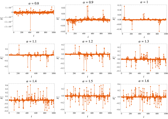
Figure 17: Mean-field converged spin configuration of the PRBM-Hubbard model with $L=1000$ and $U=1$ obtained in self-consistent numerics with different $\alpha$. In the extended phase, the local spin density is $0$ and the ground state is spin unpolarized. Near the MIT ($\alpha=1$), local magnetic moments start to form and peaks arise in the local spin densities. The density and the strength of the local moments both increases with $\alpha$. The local spin densities can be either positive or negative and the overall ferromagnetic order is absent.

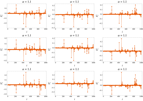
Figure 18: Mean-field converged spin configuration of the PRBM-Hubbard model with $L=1000$ and $U=1$ obtained in self-consistent numerics for $\alpha=1.1$ with different initial conditions. The positions of the local magnetic moments are almost identical for all the ground states, while the sign of their spin polarization depends on the initial conditions. The energies of all these states are nearly the same, with relative differences at the order of $10^{-5}$.