Constraints on the multiplicity of the most massive stars known: R136 a1, a2, a3, and c

Abstract

Context. The upper stellar mass limit is a fundamental parameter for simulations of star formation, galactic chemical evolution, and stellar feedback. An empirical bound on this parameter is therefore highly valuable. The most massive stars known to date are R 136 a1, a2, a3, and c within the central cluster R 136a of the Tarantula nebula in the Large Magellanic Cloud (LMC), with reported masses in excess of $150-200\,M_{\odot}$ and initial masses of up to $\approx 300\,M_{\odot}$. However, the mass estimation of these stars relies on the assumption that they are single.

Aims. Via multi-epoch spectroscopy, we provide for the first time constraints on the presence of close stellar companions to the most massive stars known for orbital periods of up to $\approx 10\,$yr.

Methods. We collected three epochs of spectroscopy for R 136 a1, a2, a3, and c with the Space Telescope Imaging Spectrograph (STIS) of the Hubble Space Telescope (HST) in the years 2020-2021 to probe potential radial-velocity (RV) variations. We combine these epochs with an additional HST/STIS observation taken in 2012. For R 136 c, we also use archival spectroscopy obtained with the Very Large Telescope (VLT). We use cross-correlation to quantify the RVs, and establish constraints on possible companions to these stars up to periods of $\approx 10\,$yr. Objects are classified as binaries when the peak-to-peak RV shifts exceed 50 km ${\rm s}^{-1}$, and when the RV shift is significant with respect to errors.

Results. R 136 a1, a2, and a3 do not satisfy the binary criteria and are thus classified as putatively single, although formal peak-to-peak RV variability on the level 40 km ${\rm s}^{-1}$ is noted for a3. Only R 136 c is classified as binary, in agreement with literature. We can generally rule out massive companions ($M_{2}\gtrsim 50\,M_{\odot}$) to R 136 a1, a2, and a3 out to orbital periods of $\lesssim 1\,$yr (separations $\lesssim 5\,$au) at 95% confidence, or out to tens of years (separations $\lesssim 100$ au) at 50% confidence. Highly eccentric binaries ($e\gtrsim 0.9$) or twin companions with similar spectra could evade detection down to shorter periods ($\gtrsim 10\,$d), though their presence is not supported by the relative X-ray faintness of R 136 a1, a2, and a3. We derive a preliminary orbital solution with a 17.2 d period for the X-ray bright binary R 136 c, though more data are needed to conclusively derive its orbit.

Conclusions. Our study supports a lower bound of $150-200\,M_{\odot}$ on the upper-mass limit at LMC metallicity.

1 Introduction

The upper mass limit of stars ($M_{\rm max}$) as a function of metallicity ($Z$) is one of the most fundamental parameters that dictate the properties of galaxies. This is because the ecology, energy budget, and integrated spectral appearance of galaxies are largely determined by the most massive stars they host ($M\gtrsim 50\,M_{\odot}$; Crowther et al., 2010; Doran et al., 2013; Ramachandran et al., 2019). Moreover, the most massive stars are invoked in the context of a plethora of unique phenomena, from pair-instability supernovae and long-duration $\gamma$-ray bursts (Fryer et al., 2001; Woosley et al., 2007; Langer, 2012; Smartt, 2009; Quimby et al., 2011; Fryer et al., 2001; Woosley et al., 2007) to the early chemical enrichment of globular clusters (Gieles et al., 2018; Bastian & Lardo, 2018). Establishing $M_{\rm max}$ from first principles or simulations of star formation is challenging due to a variety of uncertainties, and estimates vary from $\approx 120$ $M_{\odot}$ to a few $\approx 1000\,M_{\odot}$, depending on $Z$ and modelling assumptions (e.g. Larson & Starrfield, 1971; Oey & Clarke, 2005; Figer, 2005). It is therefore essential to identify and weigh the most massive stars in our Galaxy and nearby lower-metallicity galaxies such as the Small and Large Magellanic Clouds (SMC, LMC).

Stars initially more massive than ${\approx}100\,M_{\odot}$, dubbed very massive stars (VMS), tend to have emission-line dominated spectra stemming from their powerful stellar winds already on the main sequence. Such stars spectroscopically appear as Wolf-Rayet (WR) stars (de Koter et al., 1997). Being N-rich owing to the CNO burning cycle, they belong to the nitrogen WR sequence (WN). Unlike classical WR stars, which are evolved and H-depleted massive stars, VMSs typically show substantial surface hydrogen mass fractions ($X_{\rm H}\gtrsim 40\%$), and are usually classified as WNh to indicate a H-rich atmosphere.

In the case of double-lined spectroscopic binaries (SB2), the mass ratio and minimum masses of both components ($M_{1,2}\sin^{3}i$, where $i$ is the orbital inclination) can be established via Newtonian mechanics. If the inclination is known additionally, then the true masses can be derived. Best constraints are obtained for eclipsing binaries, such as the massive Galactic binaries WR 43a (Schnurr et al., 2008, $M_{1}=116\pm 31\,M_{\odot}$, $M_{2}=89\pm 16\,M_{\odot}$), WR~21a (Tramper et al., 2016; Barbá et al., 2022, $M_{1}=93\pm 2\,M_{\odot}$, $M_{2}=53\pm 1\,M_{\odot}$), WR~20a (Rauw et al., 2004; Bonanos et al., 2004, $M_{1}=83\pm 5\,M_{\odot}$, $M_{2}=82\pm 5\,M_{\odot}$), and the SMC binary HD 5980, which hosts a luminous blue variable (LBV) and a WR star of masses $60-70\,M_{\odot}$ (Koenigsberger et al., 2014). The inclination can also be constrained from interferometry (e.g., Richardson et al., 2016; Thomas et al., 2021) or from spatially resolved structures, such as the Homunculus nebula of of the Galactic binary $η$ Car, a luminous LBV+WR system with masses $\approx 100+60\,M_{\odot}$ (Madura et al., 2012; Strawn et al., 2023). Alternatively, the inclination can be constrained via polarimetry (Brown et al., 1978; Robert et al., 1992) or wind eclipses (Lamontagne et al., 1996), as was the case for the LMC binaries R 144 (alias BAT99 118) and R 145 (alias BAT99 119), which host similar-mass components with current masses of $\approx 70-80\,M_{\odot}$ and initial masses of $\approx 150\,M_{\odot}$ (Shenar et al., 2017b, 2021).

When the inclination cannot be measured, the mass ratio and minimum masses provide nevertheless important parameters, which, in conjunction with other methods, constrain the true masses of the components. Examples include the the LMC colliding-wind binary Melnick~33Na (Bestenlehner et al., 2022, $M_{1}=83\pm 19\,M_{\odot}$, $M_{2}=48\pm 11\,M_{\odot}$), and the most massive binary known to date, Melnick~34 (alias BAT99~116), with derived component masses of $M_{1}=139\pm 20\,M_{\odot}$ and $M_{2}=127\pm 17\,M_{\odot}$ (Tehrani et al., 2019).

In the absence of a companion, the mass of a star is estimated by matching the derived stellar properties (mainly the luminosity $L$, effective temperature $T_{\rm eff}$, and $X_{\rm H}$) with structure or evolution models, yielding the evolutionary current and initial masses. It is important to note that such mass estimates assume an internal structure for the star (e.g., H-burning, He-burning), which is not always trivial for WNh stars (e.g., the case of R 144, Shenar et al., 2021). Prominent examples for putatively single VMS and WNh stars include the LMC WN5h star VFTS 682 (Bestenlehner et al., 2014) and several very massive WNh and Of stars in the Galactic clusters Arches (e.g. Figer et al., 2002; Najarro et al., 2004; Martins et al., 2008; Lohr et al., 2018) and NGC~3603 (Crowther et al., 2010). The latter method was also used to establish the masses of the most massive stars known, which are the subject of this study. These stars, which are classified WN5h and which reside in the dense central cluster R 136 of the Tarantula nebula in the LMC, include R 136~a1 (alias BAT99~108, $M=200-300\,M_{\odot}$, a1 thereafter), R 136~a2 (alias BAT99 109, $M=150-250\,M_{\odot}$, a2 thereafter), R 136~a3 (alias BAT99 106, $M=150-200\,M_{\odot}$, a3 thereafter), and R136~c (alias BAT99~112, VFTS~1025, $M=150-200\,M_{\odot}$, c thereafter).

Earlier studies in the 1980s identified the central region of R 136 as a single star with a mass $\gtrsim 1000\,M_{\odot}$ (Cassinelli et al., 1981; Savage et al., 1983), but later investigations with speckle interferometry and the Hubble Space Telescope (HST) showed that the central region comprised distinct stellar sources, including a1, a2, and a3 (Weigelt & Baier, 1985; Lattanzi et al., 1994; Hunter et al., 1995). First mass measurements of these objects yielded masses of the order of $100\,M_{\odot}$ (e.g., Heap et al., 1994; de Koter et al., 1997; Massey & Hunter, 1998; Crowther & Dessart, 1998). However, Crowther et al. (2010) reported masses in excess of $200\,M_{\odot}$ using modern model atmospheres which account for iron line blanketing. Since then, the masses of a1, a2, a3, and c have been subject to several revisions (Hainich et al., 2014; Crowther et al., 2016; Rubio-Díez et al., 2017; Bestenlehner et al., 2020; Brands et al., 2022), but remain record-breaking in terms of current and initial masses. A visual companion to a1 was identified by Lattanzi et al. (1994) with the HST’s Fine Guidance Sensor (FGS), and later with HST imaging by Hunter et al. (1995). Recently, Khorrami et al. (2017) and Kalari et al. (2022) confirmed the presence of this companion, and detected another faint companion to a3 via speckle imaging. Accounting for these companions potentially lowers the mass estimates of a1 and a3 by $10-20\%$.

A drawback for mass estimates of putatively single stars is the assumption that they are single. The presence of a contaminating companion could substantially alter the derived stellar parameters (especially $L$), and, in turn, the stellar masses. The realisation that the majority of massive stars reside in binary systems (Sana et al., 2012, 2013) forces us to consider that R 136 a1, a2, a3, and c may be members of such binaries. In fact, relying on K-band spectroscopy acquired over 22 d, Schnurr et al. (2009) already identified R 136 c as a potential binary with a 8.2 d period. The relatively high X-ray luminosity ($\approx 10^{35}\,{\rm erg}\,{\rm s}^{-1}$) of R 136 c (Portegies Zwart et al., 2002; Townsley et al., 2006; Guerrero & Chu, 2008; Crowther et al., 2022) suggests that it is a colliding-wind binary, where both companions possess a fast wind, although a compact object companion is also a viable option.

Thus far, a1, a2, and a3 were not probed for multiplicity for periods longer than a few weeks. In this study, we present results from a 1.5 yr spectroscopic monitoring of R 136 a1, a2, a3, and c obtained with the Hubble Space Telescope (HST), combined with a previous epoch obtained in 2012 and archival data for R 136 c. By deriving the radial velocities (RVs) of the stars, we place constraints on potential companions. We additionally derive a new orbital solution for R 136 c. The reduction of the data is described in Sect. 2, and their analysis is described in Sect. 3. We discuss our results in Sect. 4 and provide a brief summary in Sect. 5.

2 Data and reduction

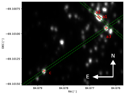
Figure 1: Image of the central 3” $\times$ 5” ($\approx 0.7\times 1.2$ parsec) core of R 136 taken in 2009 with the HST’s Wide Field Camera 3 (WFC3) in the ultraviolet and visible light (UVIS) channel with the F555W filter ($\lambda_{0}\approx 5500\,$Å, proposal ID: 11360). Marked are the positions of our four targets and the two slit positions used to acquire the data.

Our investigation relies primarily on three epochs of spectroscopy obtained with the Space Telescope Imaging Spectrograph (STIS) mounted on the HST (PI: Shenar, proposal ID: 15942). We used a slit aperture of $52^{\prime\prime}\times 0.1^{\prime\prime}$ with the G430M filter at the central wavelengths 3936 (3770-4101Å), 4706 (4540 - 4872Å), and 4961 (4795 - 5127Å). Each pair of stars (a1, a2), (a3, c) defined a STIS slit positioning to enable the acquisition of the spectra of two stars during a single pointing (Fig. 1). The resulting position angles (PA) are 106^∘ (or 286^∘) and 162.2^∘ (or 342.2^∘) for the pairs (a1, a2) and (a3, c), respectively. The PA of the pair (a1, a2) is similar to the PA used by Crowther et al. (2016) in their scanning of the R 136 cluster with STIS (where the PA was 109^∘ or 289^∘). Overall, three epochs of observations were acquired on 28 March 2020 (MJD 58936.20), 28 September 2020 (MJD 59120.07), and 14 September 2021 (MJD 59471.74) for the pair (a1, a2), and on 25 May 2020 (MJD 56023.42), 26 November 2020 (MJD 58994.06), and 14 May 2021 (MJD 59179.31) for the pair (a3, c) for each of the three spectral bands. Each exposure was divided into two dithered subexposures for removal of cosmics. The G430M filter has a spatial dispersion of 0.05”/pixel The signal-to-noise ratio (S/N) of the data is $\approx 20-80$ per pixel, depending on the star and the spectral domain. The spectral resolving power is $R=\lambda/\Delta\lambda\approx 6\,000$ with a dispersion of $\Delta\lambda=0.28\AA$.

The extraction of the spectra of the stars R 136 a3 and c across the slit is straight forward, since they are well separated spatially. The extraction of the pair (a1, a2), however, is less trivial, since the point spread functions (PSFs) of the two sources overlap (see Fig. 1). To extract the spectra, we fit Voigt profiles with identical width parameters (to mimic the PSF) to the flux across the cross-dispersion direction, as shown in Fig. 2. The fitting of the Voigt profile is performed in a wavelength-dependent fashion, such that the flux across the spatial direction was fit for each wavelength bin. We fix the separation between the Voigt profiles to 0.113” (or 2.25 HST pixels), as found by Kalari et al. (2022), and fix the amplitude ratios of the Voigt profiles to the magnitude ratio derived by Kalari et al. (2022). Avoiding the latter resulted in an instrumental wavy pattern that compromised the RV measurements. We fit for the Voigt broadening parameters $\sigma,\gamma$ as a function of wavelength, but enforce both Voigt profiles of a1 and a2 to share the same parameters. The resulting spectral energy distributions are shown in Fig. 3.

The flux levels of the four stars are relatively consistent in the three available epochs, though $\approx$10% variations are seen in a1 and a3. Such discrepancies are typical for the narrow-slit mode of STIS, which does not fully account for slit losses (e.g. Lennon et al., 2021). The overall flux level is consistent between the different epochs and is in agreement with the flux level presented by Crowther et al. (2010). However, we cannot rule out some contamination between a1 and a2 for strong lines such as He ii $\lambda 4686$ (see below), since in this case the PSFs are not well resolved. Results obtained for the He ii $\lambda 4686$ line for these components should be therefore taken with caution.

A similar technique was used by Crowther et al. (2016) for their analysis of STIS spectroscopy of the R 136 cluster. The flux-calibrated spectra show a general agreement with those presented by Crowther et al. (2016), although the underlying spectral energy distribution for a1 and a2 depends on the PA, suggesting that the flux variability observed between the epochs is linked to the observational setup rather than intrinsic. For our study, only normalised spectra were used. The extracted spectra were rectified using a homogeneous set of pre-selected continuum points.

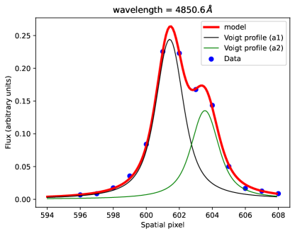
Figure 2: Fit of two Voigt profiles representing the PSFs of a1 and a2 to the flux across the cross-dispersion axis for the 28 March 2022 epoch at 4850.6$\AA$. The Voigt profiles are used to compute the relative weight of each datapoint to the flux of each star at each given wavelength.

To verify our extraction methodology, we newly extracted the spectra of a1, a2, and a3 from observations acquired in 2012 with STIS which were extracted and analysed by Crowther et al. (2016) using the multispec package (Maiz-Apellaniz, 2005; Knigge et al., 2008). The extractions match well with each other. The 2012 spectra for a1, a2, and c are combined with the newly acquired 2020-2021 spectra in our investigation to boost the binary detection probability. We also inspected the interstellar Ca ii K and H lines at 3934.77$\AA$ and 3969.59$\AA$ (wavelengths in vacuum) as a check on the absolute wavelength calibration of the spectra.

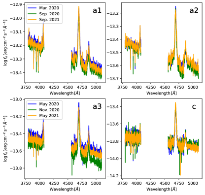
Figure 3: Extracted calibrated fluxes for a1, a2, a3, and c, for the new epochs presented here (see labels and legends).

The extracted spectra (both the new data as well as the original 2012 epochs by Crowther et al. 2016) are shown in Fig. 4. The spectra cover only few features that could correspond to cooler companions (e.g., He i $\lambda 4713$), but these features appear flat for R 136 a1, a2, and a3 (for c, see Sect. 3.2), in agreement with previous studies of these objects. We therefore only show the main diagnostic lines: N iv $\lambda 4058$, N v $\lambda\lambda 4604,4620$, He ii $\lambda 4686$, and N v $\lambda 4945$.

Before advancing to the analysis, it is interesting to already note that no clear indications for RV variability are seen from an inspection of Fig. 4, with the exception of star c. Identifying companions on the basis of spectral appearance (as opposed to RV variability) is not viable here. Companions of interest in this study would have masses $\gtrsim 50\,M_{\odot}$, and such companions show primarily H and He ii lines, which overlap with those of the WR primaries. Searching for RV variability is hence the method of choice with the available data.

For R 136 c, we use 34 archival spectra in addition to the HST data. These data cover five observing epochs (PI: Evans, ID: 182.D-0222) and were acquired in 2008-2010 with the Fibre Large Array Multi Element Spectrograph (FLAMES) ARGUS integral field unit (IFU) mounted on UT2 of the Very Large Telescope (VLT). Each spaxel of ARGUS spatially covers 0.52”. The spectra cover the range $3960-4570\,\AA$ with a resolving power of $R=10\,500$, a dispersion of $\Delta\lambda=0.2\,\AA$, and a typical S/N of 50-100 per pixel. The retrieval and reduction of the data are described in Evans et al. (2011). In addition, we retrieved a single spectroscopic observation acquired in 2001 with the Ultraviolet and Visual Echelle Spectrograph (UVES) mounted on UT2 of the VLT. We only use the spectrum covering the range 3700-5000 Å, which includes the N iv $\lambda 4058$ line. The spectrum has a resolving power of $R=40\,000$ and a S/N of $\approx 20$ per pixel, with a dispersion of $\Delta\lambda=0.015\,\AA$. The data are described in Cox et al. (2005), and are retrieved in reduced form from the European Southern Observatory’s (ESO) archive. We ensure wavelength calibration to within a few km ${\rm s}^{-1}$ using the Ca ii H line at 3969.59$\AA$, which is present in the HST, ARGUS, and UVES datasets.

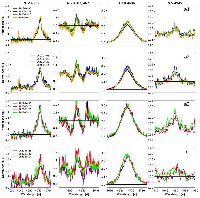
Figure 4: Extracted STIS spectra for a1, a2, a3, and c (from top to bottom), focusing on the diagnostic lines N iv $\lambda 4058$, N v $\lambda\lambda 4604,4620$, He ii $\lambda 4686$, and N v $\lambda 4945$ (from left to right). Epochs are listed in the legends. The spectra of a3 and c are binned at $\Delta\lambda=0.5\,\AA$ for clarity.

3 Analysis

3.1 Cross correlation

The main tool with which our targets are probed for multiplicity is the measurement of RVs via maximisation of cross-correlation functions (CCF). The technique is described by Zucker & Mazeh (1994), and is frequently implemented for WR binaries (e.g., Shenar et al., 2017b, 2019, 2021; Dsilva et al., 2020, 2022, 2023). Briefly, the CCF is computed in a particular spectral range (or multiple ranges) as a function of Doppler shift using a pre-specified template that should represent the star. While for WR stars the template is usually produced by co-adding the individual observations, this does not yield satisfactory results in our case due to the limited number of observations and the modest S/N. Moreover, we refrain from cross-correlating multiple lines simultaneously, since lines in WR spectra are formed in different radial layers and therefore often produce systematic shifts with respect to one another (e.g. Shenar et al., 2017a). Instead, we use a synthetic spectrum computed with the Potsdam Wolf-Rayet (PoWR) model atmosphere code (Hamann & Gräfener, 2003; Sander et al., 2015) tailored for the analysis of these objects by Hainich et al. (2014). While this yields absolute RVs, an absolute RV calibration for WR stars is highly model dependent since the line centroids sensitively depend on the atmosphere parameters. However, this does not impact our study, since the detection of binaries relies on relative RVs. A comparison between the PoWR model used here and the spectrum of a1 is shown in Fig. 5.

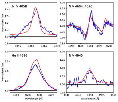
Figure 5: Comparison between the synthetic PoWR model (solid red line) used for cross-correlation and the normalised spectrum of a1 taken in March 2020 (noisy blue line). The line profiles of the PoWR model were shifted by 330 km ${\rm s}^{-1}$ and the equivalent widths of the N iv $\lambda 4058$ and N v $\lambda 4945$ profiles were scaled to the observations for the sake of plotting (the equivalent width has no impact on the cross-correlation algorithm). The spectra of a2, a3, and c are comparable, and so is the match between the model and the data.

The results from the CCF analysis for N iv $\lambda 4058$, N v $\lambda\lambda 4604,4620$, He ii $\lambda 4686$, and N v $\lambda 4945$ are shown in Fig. 6. Tables 2 and 3 in Appendix A provide a compilation of these measurements and the measured EWs of these lines. Upper bounds on the statistical errors on the EWs are computed as in Chalabaev & Maillard (1983). Significant EW variability is noted between the 2012 epoch and the other epochs in the He ii $\lambda 4686$ line belonging to a1. While such variability is not untypical for WR stars (e.g., Moffat & Bobert, 1992; Lépine & Moffat, 1999), this result could also be spurious given the difficulty in the more challenging extraction of the He ii $\lambda 4686$ line (see Sect. 2.

While the nitrogen lines are typically considered as the best RV probes of WN stars as they form relatively close to the stellar surface, the modest S/N becomes a limiting factor. In this context, the He ii $\lambda 4686$ line offers an important high S/N RV probe, but its interpretation should be treated with caution for a1 and a2 given possible cross-contamination in this line. The fact that the RVs of a1 and a2 from the N iv $\lambda 4058$, N v $\lambda\lambda 4604,4620$, and N v $\lambda 4945$ lines are consistent between the epochs, but the those of the He ii $\lambda 4686$ line are strongly variable, suggests that this RV variability is not genuine.

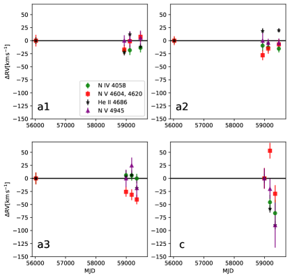
Figure 6: Relative RVs measured for the four diagnostic spectral features in the spectra (when available; see legend). The first RV is always calibrated to zero. Only component c is classified as binary by fulfilling Eqs. (1) and (2).

In principle, to classify RV variables into binaries vs. putatively single, one commonly adopts a significance criteria on the peak-to-peak RV variability (see, e.g., Sana et al. 2013). Due to the intrinsic variability of WR stars, it is often not trivial to find a single criterion. A significance criterion on the peak-to-peak (pp) RV shift which is commonly adopted is

$$\Delta{\rm RV}_{\rm pp,\sigma}=\underset{i\neq j}{\rm max}\left\{\frac{\left|{\rm RV}_{i}-{\rm RV}_{j}\right|}{\sqrt{\sigma_{i}^{2}+\sigma_{j}^{2}}}\right\}>4,$$ (1)

where $\sigma$ is the corresponding error on the RV measurement. The threshold 4 is considered conservative, resulting in a false-positive probability of roughly 0.1% (Sana et al., 2013). However, because of the intrinsic variability of WR stars, $\sigma$ may be underestimated, and this criterion alone can lose validity. Hence, in addition, we also invoke a threshold criterion on the peak-to-peak RV difference, $\Delta{\rm RV}_{\rm pp}={\rm max}\{{\rm RV}_{i}-{\rm RV}_{j}\}$. Dsilva et al. (2023) conducted an RV monitoring survey of 11 late-type WN stars of spectral classes similar to those of a1, a2, a3, and c, and found the threshold $\Delta{\rm RV}_{\rm pp}>50\,$km ${\rm s}^{-1}$ clearly separated spectroscopic binaries from potentially single stars, and that intrinsic variability can lead to apparent RV variations of up to $50\,$km ${\rm s}^{-1}$, depending on the wind and stellar properties. Our second criterion for a binary classification is thus:

$$\Delta{\rm RV}_{\rm pp}=\underset{i\neq j}{\rm max}\left|{\rm RV}_{i}-{\rm RV}_{j}\right|>50\,{\rm km}\,{\rm s}^{-1}$$ (2)

While the choice of this threshold impacts our classification to binary or single, the bias discussion provided in Sect. 4 addresses this issue. Table 1 summarises whether or not Eqs. (1) and (2) are fulfilled for each of the spectral diagnostics. When both conditions are satisfied, we flag the star as binary. Evidently, the only star that satisfies both conditions is R 136 c (with the He ii $\lambda 4686$ line, and marginally with the nitrogen lines). In contrast, a1, a2, and a3 do not satisfy both conditions for any of the lines, and are hence flagged as putative single. The fact that R 136 c is classified as binary is consistent with the findings of Schnurr et al. (2009), who derived a tentative 8.2 d orbital period for this object, and its high X-ray luminosity, suggestive of colliding winds or a compact object in the binary (Portegies Zwart et al., 2002; Crowther et al., 2022).

Table 1: Binary status of R 136 a1, a2, a3, and c

Object	Condition	N iv $4058$	N v $4603,4621$	He ii $4686$	N v $4945$
a1	Eq. (1)	no	no	yes (a)	no
a1	Eq. (2)	no	no	no	no
a1	binary?	no	no	no	no
a2	Eq. (1)	no	no	yes (a)	no
a2	Eq. (2)	no	no	no	no
a2	binary?	no	no	no	no
a3	Eq. (1)	no	no	no	no
a3	Eq. (2)	no	no	no	no
a3	binary?	no	no	no	no
c	Eq. (1)	no	no	yes	no
c	Eq. (2)	yes	yes	yes	yes
c	binary?	no	no	yes	no

Before advancing to the interpretation of these results, one may wonder whether a 1D CCF method is valid if these objects are double-lined spectroscopic binaries (SB2). Given the spectral appearance of our targets, the only companions which could be relevant in terms of contributing sufficient flux to bias the results are O-type stars or WR stars. O-type dwarfs typically have absorption-line dominated spectra with weak to non-existing features belonging to N iv or N v, and much weaker features in the He ii $\lambda 4686$ line compared to a WR star (Walborn & Fitzpatrick, 1990; Walborn et al., 2002). A contamination with an O dwarf therefore poses no danger to our RV measurement methodology.

However, a contamination with an Of star, a transition O/WR star (Crowther & Walborn, 2011), or a WN star could impact our interpretation. For example, consider the case of two WN stars with similar N iv $\lambda 4058$ or He ii $\lambda 4686$ line profiles. Typical peak-to-peak RV amplitudes may fall below the full-width half-maximum (FWHM) of these lines, implying that the line profiles would remain blended and show a marginal or even vanishing RV shift (e.g., Sana et al., 2011). The same argument holds for P-Cygni lines (such as N v $\lambda\lambda 4604,4620$), although the effect is more difficult to quantify. Thus, instead of an RV variation, one would observe a periodic change in the FWHM of the line. Excess emission stemming from wind-wind collisions (WWC) may also be added to this line, further changing its profile (Luehrs, 1997). For this reason, we also measured the FWHMs of the N iv $\lambda 4058$ and He ii $\lambda 4686$ lines for the a1, a2, a3, and c (Fig. 7). To obtain the FWHMs and their respective errors, we fit Gaussian profiles to the N iv $\lambda 4058$ and He ii $\lambda 4686$ lines and generate 1000 spectra with the same underlying Gaussian profile and S/N of the original data. The FWHM is then taken as the average of the FWHMs of these 1000 simulated spectra, and the error is their standard deviation. The results are shown in Fig. 7, and are also provided in Table 4. Neither of the stars exhibits strong variability, with only the He ii $\lambda 4686$ line of R 136 c being significantly variable (on a 4$\sigma$ level). The interpretation of these results will be conducted in Sect. 4.

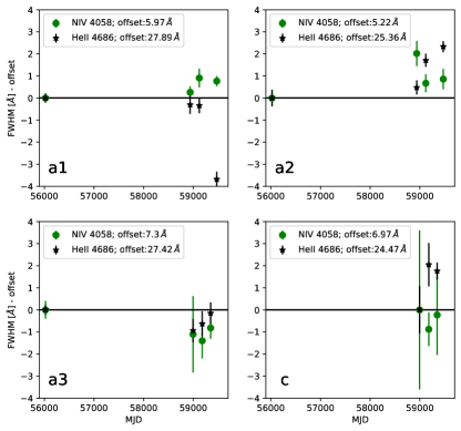
Figure 7: FWHMs of the N iv $\lambda 4058$ and He ii $\lambda 4686$ lines for components a1, a2, a3, and c. The values are offset relative to the FWHMs measured in the first available epoch for each star. The offset values are provided in the legend. Only the FWHMs of He ii $\lambda 4686$ for component c are significantly variable (on a 4$\sigma$ level).

3.2 Orbital analysis of R 136 c

We follow a similar analysis methodology using the 34 calibrated FLAMES spectra and single UVES spectrum available for R 136 c, which probe six distinct observational epochs in addition to the three HST epochs. The only robust RV probe in the available spectral range is the N iv $\lambda 4058$ line, for which the same PoWR template is used as in Sect. 3.1. The full list of RVs is available in Tables 2 and 5. The amplitude of the RV variability is in apparent agreement with the HST data.

Figure 8 shows a Lomb-Scargle periodogram derived for the full set of RVs (HST + FLAMES + UVES). Evidently, multiple peaks are present in the periodogram, with the most prominent peaks at $P=5.277,5.345,5.563,17.20,25.94,47.15$, and $83.06\,$d. For this set of periods, we use Python’s lmfit minimisation package with the differential evolution method to constrain the time of periastron $T_{0}$, systemic velocity $V_{0}$, RV semi amplitude $K_{1}$, argument of periastron $\omega$, and eccentricity $e$ via

$${\rm RV}(\nu)=V_{0}+K_{1}\,\left(\cos\nu+e\,\cos\omega\right).$$ (3)

The lowest reduced $\chi^{2}$ (reduced $\chi^{2}=0.46$) is obtained for $P=17.20$ d, which is refined to $P=17.2051\,$d during the minimisation. We obtain: $T_{0}=54737.8\pm 1.5$ [MJD], $V_{0}=307.6\pm 2.8$ km ${\rm s}^{-1}$, $K_{1}=51\pm 9\,$km ${\rm s}^{-1}$, $\omega=148.5\pm 3.7^{\circ}$, $e=0.31\pm 0.08$. Figures 9 and 10 compare this solution to the measurements. However, that acceptable solutions are found for all the periods listed above. We tried combining these RVs with those published by Schnurr et al. (2009) from IR data, but the period remains poorly constrained. Since the analysis involved a different spectral line than N iv $\lambda 4058$, we refrain from including the RVs from Schnurr et al. (2009) in our final analysis. Moreover, the preliminary 8.2 d period derived by Schnurr et al. (2009) is not supported by our analysis.

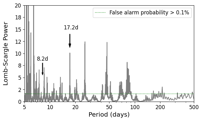
Figure 8: Lomb-Scargle periodogram of the full RV set derived from the HST + FLAMES + UVES data for R 136 c. Our favoured period of 17.2 d is marked, along with the previously published 8.2 d period, which is not supported by this study.

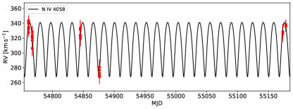
Figure 9: The RVs measured for the FLAMES/ARGUS data for R 136 c as a function of MJD, compared to the best-fitting RV curve corresponding to $P=17.2051\,$d.

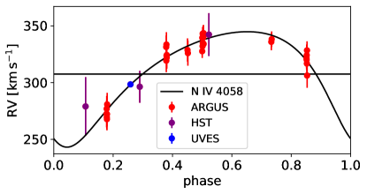
Figure 10: As Fig. 9, but plotted as a function of phase and including the HST data and UVES datapoints.

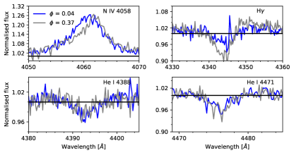
Figure 11: Comparison of ARGUS spectra of R 136 c taken during RV extremes, illustrating the apparent motion of the N iv $\lambda 4058$ line and the presence of seemingly static He i absorption lines.

Another interesting fact is the presence of He i absorption lines in the spectrum of R 136 c (Fig. 11). These He i lines are seemingly static. The standard deviation of their RVs is 9.3 km ${\rm s}^{-1}$, comparable with the mean of the statistical error (7.7 km ${\rm s}^{-1}$). If these lines originate in the physical companion of the WR star in R 136 c, then it must be a few times more massive than the WR star to avoid observed RV variability. This is somewhat in tension with the spectral type of the object, which is suggestive of a late-type O star or an early type B star. More likely, these lines belong to a distant tertiary source. Hénault-Brunet et al. (2012) noted that the ARGUS spaxel (which covers 0.52”, Sect. 2) included two sources, with R 136 c being significantly brighter. It is well possible that the second star produces the He i absorption lines.

The H$\gamma$ line shown in Fig. 11 likely stems from both the WN5h component and the late OB-type component. However, the variability seen in Balmer lines such as H$\gamma$ is likely dominated by the WNh5 component and its motion. WN5h stars, including a1, a2, and a3, typically show a combined emission+absorption profile in H$\beta$, H$\gamma$, and H$\delta$ (Crowther et al., 2010). Additional variability could stem from wind-wind collisions (e.g. Hill et al., 2000), although this remains speculative without knowledge of the nature of the companion of the WN5h component.

The nature of the secondary in R 136 c thus remains unclear, and, in light of the discrepant RVs among the spectral lines (Fig. 6) and the multiple possible periods (Fig. 8), more data will be necessary to unambiguously derived the orbit. The fact that it is X-ray bright (Portegies Zwart et al., 2002) implies that the secondary is either another star with a strong wind (presumably an Of star or a WR star), or a compact object.

4 Discussion

We can use the RVs measured in Sect. 3 to place constraints on possible companions to a1, a2, a3, and c. We use the RVs obtained for the N iv $\lambda 4058$ line, which has the smallest measurement errors after the He ii $\lambda 4686$ line, for which cross-contamination between a1 and a2 cannot be ruled out. We perform Monte Carlo simulations to estimate the likelihood of specific binary configurations in reproducing the observed peak-to-peak RV variability. Specifically, for each pair of period $P$ and companion mass $M_{2}$ in the range $0.3\leq\log P[\,{\rm d}]\leq 4.5$ and $2\leq M_{2}\,[M_{\odot}]\leq 150$, respectively, we draw 1000 binaries from the following distributions: the eccentricities are drawn from a Gaussian distribution with a mean of 0.3 and a standard deviation of 0.2. In Appendix B, we explore the impact of highly eccentric binaries. The primary mass is drawn from a uniform distribution in the range $100-300\,M_{\odot}$, the inclination $i$ is drawn uniformly on $\cos i$ (corresponding to a random orientation of the orbital plane), the argument of periastron $\omega$ is drawn uniformly in the range $0-2\,\pi$, and the time of periastron $T_{0}$ is drawn uniformly in the interval $0-P$. The mass range $100-300\,M_{\odot}$ for the primaries is justified by WNh classification of our targets, which typically corresponds to $M\gtrsim 100\,M_{\odot}$, as well as by their previous mass determinations. For each star and for each mock binary, the RVs are computed using the actual dates of observations for that star. For each mock binary, the errors on the set of RVs are assumed to be identical to the actual measured errors, and the mock RVs are modified assuming these errors. Like this, we form a series of 1000 peak-to-peak measurements corresponding to Eqs. (1) and (2) for each $P,M_{2}$ pair.

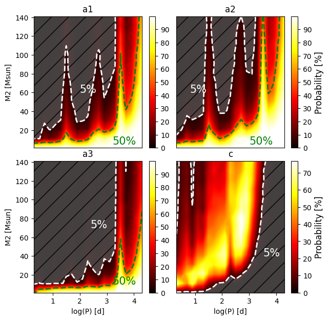
Figure 12: Allowed configurations for companions for a1, a2, a3, and c using the RV measurements for the N iv $\lambda 4058$ line. The panels for a1, a2, and a3, which were not classified as binaries here, show the probability of a binary with the given $M_{2},P$ to produce values of $\Delta{\rm RV}_{{\rm pp},\sigma}$ and $\Delta{\rm RV}_{{\rm pp}}$ below our observed values. The 5% and 50% thresholds are marked. For star c, which is classified as binary here, shown is the probability that a binary in the given configuration would reproduce the observed $\Delta{\rm RV}_{\rm pp}$ within $\pm\sqrt{\sigma_{i}^{2}+\sigma_{j}^{2}}$. Only 5% thresholds are marked for clarity (see text for details).

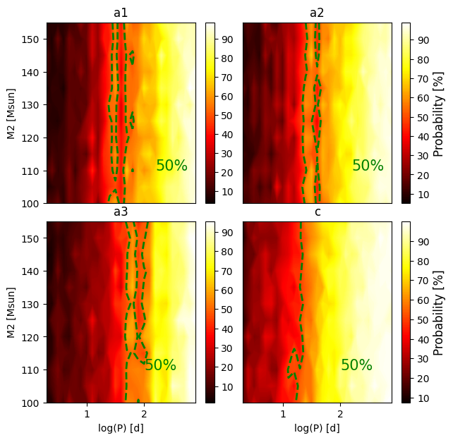
Figure 13: Allowed configurations for companions for a1, a2, a3, and c for the case of two WR stars with identical spectra. Shown are the probabilities that the ratios between the largest and smallest FWHM values for the N iv $\lambda 4058$ line are less than the observed values (Fig. 7). The 5% and 50% thresholds are marked. The probabilities drop sharply in comparison with the RV case (Fig. 12 ). See text for details.

Since stars a1, a2, and a3 are not flagged as binaries in our study, for these stars, Fig. 12 shows the probability that a binary of a given $P,M_{2}$ would yield values of $\Delta{\rm RV}_{{\rm pp},\sigma}$ and $\Delta{\rm RV}_{{\rm pp}}$ that are lower than those observed here for the N iv $\lambda 4058$ line. The shaded areas correspond to configurations that can be rejected at 95% probability, corresponding to the probability of such binaries to produce peak-to-peak RV variations larger than those observed. The probabilities for star c, which was flagged as binary in our study, are discussed below. Evidently, companions with masses $M_{2}\lesssim 10\,M_{\odot}$ (corresponding to mass ratios $\lesssim 0.1$) cannot be ruled out at arbitrarily short periods. However, since our main focus is companions that could contribute significantly to the flux and bias the original mass estimates of these components, it is fair to focus our attention to $M_{2}\gtrsim 50\,M_{\odot}$. For such stars, we can confidently rule out companions up to periods of a few years (separations $a\lesssim 10\,$au) at 95% confidence, and up to tens of years ($a\lesssim 100\,$au) at 50% confidence, unless the periods coincide with one of the aliases of the limited HST time series. Constraints for a3 are somewhat less stringent.

Kalari et al. (2022) obtained Speckle imaging of the R 136 cluster and identified a companion at a projected separation of 2000 au to a1 and a3, the former of which also identified by Lattanzi et al. (1994), Hunter et al. (1995), and Khorrami et al. (2017). From figure 1 in Kalari et al. (2022), we expect their study to be sensitive down to $\approx 1000\,$au. Hence, in conjunction with Kalari et al. (2022), we cannot exclude massive companions in the range $10\lesssim a\,[{\rm au}]\lesssim 1000$.

For star c, Fig. 12 shows the probability as a function of $P,M_{2}$ that a star would reproduce the observed peak-to-peak variability. Specifically, we require that $\left|\Delta{\rm RV}_{\rm pp,mock}-\Delta{\rm RV}_{\rm pp,obs}\right|<\sqrt{\sigma_{i}^{2}+\sigma_{j}^{2}}$, where $\sigma_{i},\sigma_{j}$ are the errors on the RVs which produce $\Delta{\rm RV}_{\rm pp,obs}$. This limits, within 95% confidence, the range of acceptable companion masses and periods to R 136 c. The results are consistent with the period of 17.20 d derived in our study.

Finally, we consider the case of two WR-like stars with similar line profiles and light contributions, and consider the FWHM variability that could be expected in this case (see discussion in Sect. 3). We focus on the N iv $\lambda 4058$ line, to prevent possible cross-contamination between a1 and a2 in the He ii $\lambda 4686$ line impacting our results. Like the exercise above, for each pair of $M_{2},P$, we draw 1000 binaries following the same distributions as before, focusing on $100\leq M_{2}/M_{\odot}\leq 150$ and $0.3\leq\log P\,[{\rm d}]\leq 3$. We fit the underlying N iv $\lambda 4058$ profile of a1, a2, a3, and c with Gaussians. Then, we compute the FWHM of a Gaussian comprising of the sum of two such Gaussians that are shifted relative to one another by $\Delta{\rm RV}$. We fit a quadratic function to FWHM($\Delta{\rm RV}$) to obtain an analytical relation between the FWHM and $\Delta{\rm RV}_{\rm pp}$ for each star. For each $\Delta{\rm RV}_{\rm pp}$ value in a given simulation of a $M_{2},P$ pair, we classify the mock binary as binary if the ratio of the FWHM of the N iv $\lambda 4058$ line to that of the unshifted Gaussian exceeds the values we observe. The results are shown in Fig. 13.

Evidently, the probability to detect companions with similar spectra sharply drops in comparison with binaries containing only one WR star. Only very short period ($\lesssim 3\,$d) can be rejected at high probability (90%); the 50% thresholds lie at periods of the order of 10-100 d. The results are insensitive to $M_{2}$, recalling that the underlying assumption here is that the two stars have similar spectra. If the secondary is significantly fainter or does not show N iv $\lambda 4058$ or He ii $\lambda 4686$ in emission, then the RVs become a sensitive probe, and Fig. 12 becomes the relevant diagnostic. We conclude that close companions of a similar spectral type cannot be readily excluded from the current data. A longer time coverage and higher data quality should allow for more stringent constraints in this case.

The absence of strong X-ray emission in a1, a2, and a3 does not favour the presence of close massive companions. For example, the X-ray luminosity of the WN5+WN5 binary Mk 34, with orbital period of 155 d, is $\approx 10^{35}\,{\rm erg}\,{\rm s}^{-1}$ (Pollock et al., 2018; Tehrani et al., 2019), which exceeds the combined X-ray luminosity of a1, a2, and nearby targets by an order of magnitude (Crowther et al., 2022). However, the colliding wind phenomenon occurs only in a subset of massive binaries – the X-ray emission of a majority of known spectroscopic binaries does not exceed average value $L_{\rm X}/L_{\rm bol}\sim 10^{-7}$ (Oskinova, 2005; Sana et al., 2006; Rauw & Nazé, 2016; Nebot Gómez-Morán & Oskinova, 2018; Crowther et al., 2022). For example, R 144 is a colliding-wind binary hosting two WR stars bound on a 74 d period which does not exhibit strong X-ray excess (Shenar et al., 2021). Nazé (2009) noted that, for the short period massive binaries ($P_{\rm orb}\lesssim 30$ d), the prevalence of enhanced X-rays is lower compared to longer period binaries. The physical reason could be the braking of stellar winds by the radiation of companions in close binaries which dramatically reduces the strength of the wind collision (Gayley et al., 1997), or that the collision occurs withing the wind acceleration zone (Sana et al., 2004). Furthermore, Krtička et al. (2015) suggest that intrinsic X-ray emission could lead to wind inhibition in massive binaries. Hence, generally, while X-ray excess provides indirect support for a companion with a powerful wind, lack of X-ray excess does not suffice to reject such a companion.

5 Summary

We investigated whether some of the most massive stars reported to date – R 136 a1, a2, a3, and c – may be binaries that host two massive stars, which would affect their previous mass determinations. To this end, we collected three epochs of optical spectroscopy over 1.5 yr in the years 2020-2021 with the STIS instrument on the HST to search for RV and EW variations or other indications for binary motion. These data were combined with an additional epoch in 2012 acquired by Crowther et al. (2016) to form a 10-year baseline for our study. For R 136 c, we combined these data with archival FLAMES and UVES data to derive a preliminary orbital solution.

The data are not readily suggestive of close companions to the stars a1, a2, or a3. We can rule out companions more massive than $\approx 50\,M_{\odot}$ out to orbital periods $\lesssim 1-3$ years ($a\lesssim 5-10\,$au) at 95% confidence, or periods of tens of years ($a\lesssim 100\,$au) at 50% confidence. In conjunction with previous imaging studies (Khorrami et al., 2017; Kalari et al., 2022), additional companions could only reside in the range $\approx 10-1000\,$au. However, ”twin companions” with similar light contributions and spectral appearance could avoid detection down to much shorter periods ($P\gtrsim 10\,$d), though no direct indications for such companions (e.g., from the spectral appearance or X-ray behaviour) are noted. Hence, the masses of a1, a2, and a3 may still be considered to be $\gtrsim 150\,M_{\odot}$ (Crowther et al., 2010; Bestenlehner et al., 2020; Brands et al., 2022), although the faint visual companions to a1 and a3 (Hunter et al., 1995; Kalari et al., 2022) may lead to a modest downward revision of the masses.

In contrast, R 136 c is classified as a binary in our study. This is consistent with previous indications for binarity reported by Schnurr et al. (2009) and Hénault-Brunet et al. (2012) , who reported this object to be a binary candidate based on IR and VIS spectroscopy. Combining archival data with the new one, we propose a tentative period of 17.2 d for R 136 c, though more data will be needed to robustly constrain the orbital configuration and the true nature of the companion. Given the X-ray brightness of the system and the rarity of such very massive binaries, future monitoring of R 136 c would yield important constraints on the masses of the most massive stars and on massive binary evolution.

Appendix A Observation log and RV measurements

Tables 2 and 5 compile the RV measurements for a1, a2, a3, and c using the STIS/HST data and the ARGUS/FLAMES data, respectively. Table 3 compiles the EWs of several lines in the STIS/HST data, while Table 4 provides the FWHM of the N iv $\lambda 4058$ and He ii $\lambda 4686$ lines for the STIS/HST dataset.

Table 2: RVs (in ${\rm km}\,{\rm s}^{-1}$) for a1, a2, a3, and c, as derived from the STIS/HST data

Object	MJD	S/N	RV (N iv $4058$)	RV (N v $\lambda\lambda 4603,4621$)	RV (He ii $\lambda 4686$)	RV(N v $\lambda 4945$)
a1	56023.44	36	354.4 $\pm$ 6.2	327.1 $\pm$ 11.2	307.6 $\pm$ 6.2	-
	58936.20	36	335.0 $\pm$ 7.3	310.0 $\pm$ 9.1	285.4 $\pm$ 6.0	346.7 $\pm$ 10.3
	59120.06	47	336.1 $\pm$ 9.2	325.9 $\pm$ 10.0	319.6 $\pm$ 5.5	348.3 $\pm$ 16.4
	59471.74	34	340.6 $\pm$ 8.7	334.5 $\pm$ 9.6	296.0 $\pm$ 5.3	352.1 $\pm$ 13.9
a2	56023.84	134	350.9 $\pm$ 6.5	335.2 $\pm$ 8.4	220.3 $\pm$ 4.0	-
	58936.20	29	341.4 $\pm$ 10.3	307.2 $\pm$ 9.5	239.0 $\pm$ 5.0	356.8 $\pm$ 14.7
	59120.07	64	337.7 $\pm$ 8.5	320.1 $\pm$ 9.9	215.5 $\pm$ 3.7	352.5 $\pm$ 7.8
	59471.73	38	335.5 $\pm$ 7.1	328.1 $\pm$ 10.0	240.2 $\pm$ 4.0	352.3 $\pm$ 8.6
a3	56023.42	33	341.3 $\pm$ 11.3	301.9 $\pm$ 11.4	231.1 $\pm$ 4.3	-
	58994.06	21	347.3 $\pm$ 9.4	276.2 $\pm$ 9.4	234.5 $\pm$ 5.2	334.3 $\pm$ 16.5
	59179.31	19	346.9 $\pm$ 9.9	270.6 $\pm$ 10.4	237.4 $\pm$ 5.8	359.1 $\pm$ 15.0
	59348.22	42	341.0 $\pm$ 9.0	261.5 $\pm$ 9.2	212.8 $\pm$ 4.7	315.7 $\pm$ 23.7
c	58994.06	14	393.1 $\pm$ 19.1	290.0 $\pm$ 20.0	333.7 $\pm$ 8.5	393.4 $\pm$ 19.4
	59179.31	19	347.4 $\pm$ 14.3	343.0 $\pm$ 15.0	275.5 $\pm$ 7.4	373.4 $\pm$ 19.3
	59348.22	14	326.4 $\pm$ 25.5	260.4 $\pm$ 16.5	244.1 $\pm$ 7.9	303.8 $\pm$ 43.1

Table 3: EWs for diagnostic lines of a1, a2, a3, and c, as derived from the STIS/HST data (in units of $\AA$) ^(a)

Object	MJD	EW (N iv $4058$)	EW (N v $\lambda\lambda 4603,4621$)	EW (He ii $\lambda 4686$)	EW(N v $\lambda 4945$)
a1	56023.44	-2.1$\pm 0.4$	0.5$\pm 0.5$	-30.8$\pm 0.9$	-
	58936.20	-2.2$\pm 0.5$	0.1$\pm 0.6$	-38.5$\pm 2.4$	-0.22$\pm 0.08$
	59120.06	-2.4$\pm 0.7$	-0.1$\pm 0.7$	-35.0$\pm 1.5$	-0.15$\pm 0.05$
	59471.74	-2.8$\pm 1.2$	0.8$\pm 0.9$	-36.6$\pm 2.5$	-0.07$\pm 0.08$
a2	56023.84	-1.7$\pm 0.4$	0.5$\pm 0.4$	-33.8$\pm 1.8$	-
	58936.20	-2.4$\pm 0.7$	0.4$\pm 0.7$	-40.8$\pm 1.4$	-0.33$\pm 0.09$
	59120.07	-2.2$\pm 0.6$	0.1$\pm 0.6$	-37.5$\pm 1.3$	-0.42$\pm 0.10$
	59471.73	-2.1$\pm 0.7$	0.8$\pm 0.6$	-37.9$\pm 2.4$	-0.22$\pm 0.08$
a3	56023.42	-3.0$\pm 1.0$	0.7$\pm 0.5$	-52.8$\pm 1.6$	-
	58994.06	-3.7$\pm 1.6$	0.5$\pm 1.5$	-58.3$\pm 4.5$	-0.41$\pm 0.09$
	59179.31	-3.0$\pm 1.3$	1.1$\pm 2.1$	-55.1$\pm 6.1$	-0.40$\pm 0.12$
	59348.22	-3.0$\pm 1.1$	-1.0$\pm 1.5$	-58.0$\pm 5.4$	-0.68$\pm 0.13$
c	58994.06	-2.4$\pm 1.8$	1.3$\pm 2.5$	-48.0$\pm 6.3$	-0.12$\pm 0.08$
	59179.31	-2.5$\pm 1.0$	-2.3$\pm 3.0$	-55.9$\pm 4.7$	-0.43$\pm 0.08$
	59348.22	-2.9$\pm 1.3$	-0.5$\pm 2.7$	-53.2$\pm 5.1$	-0.24$\pm 0.11$

Table 4: FWHMs (in Å) of the N iv $\lambda 4058$ and He ii $\lambda 4686$ lines in the STIS/HST datasets

Object	MJD	FWHM (N iv $\lambda 4058$)	FWHM (He ii $\lambda 4686$)
a1	58936.20	6.33$\pm 0.51$	27.26$\pm 0.37$
	59471.74	7.18$\pm 0.83$	24.77$\pm 0.46$
	59120.06	6.80$\pm 0.57$	25.69$\pm 0.40$
	56023.44	5.81$\pm 0.37$	27.60$\pm 0.37$
a2	58936.20	7.60$\pm 0.94$	25.83$\pm 0.42$
	59120.07	6.42$\pm 0.51$	27.13$\pm 0.52$
	56023.84	5.65$\pm 0.39$	24.90$\pm 0.37$
	59471.73	6.37$\pm 0.59$	27.56$\pm 0.39$
a3	58994.06	6.74$\pm 0.84$	26.55$\pm 0.52$
	59348.22	6.67$\pm 0.75$	26.59$\pm 0.56$
	56023.42	7.58$\pm 0.41$	27.79$\pm 1.28$
	59179.31	6.43$\pm 0.67$	26.77$\pm 0.52$
c	58994.06	7.66$\pm 1.92$	24.90$\pm 0.67$
	59179.31	6.50$\pm 1.26$	26.39$\pm 0.58$
	59348.22	8.24$\pm 1.41$	26.05$\pm 0.62$

Table 5: RVs (in ${\rm km}\,{\rm s}^{-1}$) for R 136 c, as derived from the UVES and FLAMES data

Instrument	MJD	S/N	RV (N iv $4058$)
UVES	52176.296	40	298.5 $\pm$ 2.2
FLAMES	54761.217	86	327.7 $\pm$ 5.9
FLAMES	54761.224	46	339.5 $\pm$ 5.9
FLAMES	54761.230	57	339.6 $\pm$ 6.6
FLAMES	54761.237	43	332.1 $\pm$ 5.6
FLAMES	54761.244	97	343.2 $\pm$ 6.0
FLAMES	54761.251	76	335.1 $\pm$ 5.7
FLAMES	54761.267	35	340.4 $\pm$ 6.4
FLAMES	54761.273	117	339.7 $\pm$ 6.2
FLAMES	54761.280	51	340.6 $\pm$ 5.5
FLAMES	54761.287	39	342.5 $\pm$ 7.8
FLAMES	54761.293	59	343.6 $\pm$ 7.2
FLAMES	54761.300	75	334.1 $\pm$ 7.0
FLAMES	54767.263	93	321.5 $\pm$ 8.1
FLAMES	54767.270	76	320.2 $\pm$ 8.6
FLAMES	54767.277	79	324.1 $\pm$ 9.4
FLAMES	54767.283	110	316.8 $\pm$ 8.0
FLAMES	54767.290	67	328.4 $\pm$ 7.9
FLAMES	54767.297	23	306.2 $\pm$ 10.8
FLAMES	54845.157	59	331.4 $\pm$ 10.1
FLAMES	54845.163	109	319.4 $\pm$ 10.2
FLAMES	54845.170	69	333.6 $\pm$ 10.9
FLAMES	54845.177	70	323.8 $\pm$ 9.7
FLAMES	54845.183	57	321.9 $\pm$ 9.8
FLAMES	54845.190	36	324.4 $\pm$ 11.8
FLAMES	54876.111	75	272.5 $\pm$ 11.9
FLAMES	54876.118	65	276.9 $\pm$ 11.3
FLAMES	54876.124	134	269.6 $\pm$ 10.2
FLAMES	54876.131	60	267.8 $\pm$ 9.8
FLAMES	54876.138	38	272.2 $\pm$ 10.8
FLAMES	54876.144	122	280.8 $\pm$ 10.2
FLAMES	55173.288	210	328.7 $\pm$ 10.2
FLAMES	55173.310	144	326.0 $\pm$ 11.1
FLAMES	55178.145	183	335.9 $\pm$ 7.4
FLAMES	55178.167	95	338.3 $\pm$ 6.8

Appendix B Detection probabilities for highly eccentric binaries

Some known massive binaries in the LMC exhibit high eccentricities (e.g., R 145, $e=0.79$, Shenar et al. 2017a; R 144, $e=0.56$, Shenar et al. 2021; Mk 34, $e=0.76$, Tehrani et al. 2019), while others exhibit more moderate eccentricities (e.g., Mk 33Na, $e=0.33$, Bestenlehner et al. 2022; R~139, $e=0.38$, Taylor et al. 2011; Mahy et al. 2020). To explore the impact of potential high eccentricity in our targets, we repeat the exercise performed in Sect. 4 for a Gaussian eccentricity distribution with a mean of $\langle e\rangle=0.8$ and a standard deviation of 0.1 (Fig. 14). As could be anticipated, the detection probability drops, though the exclusion domains are still comparable. Only highly eccentric binaries ($e>0.9$) would have an appreciable likelihood to evade detection even at shorter ($\lesssim 100\,$d) orbital periods. More epochs would certainly improve the detection probability of high eccentricity binaries.

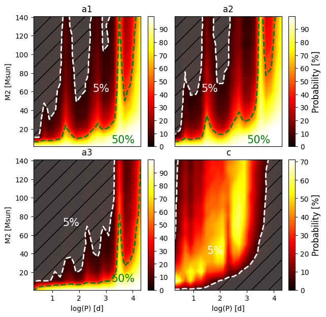
Figure 14: As Fig. 12 but for an underlying Gaussian eccentricity distribution with a mean of $<e>=0.8$ and standard deviation of 0.1