Distributed Optimisation with Linear Equality and Inequality Constraints using PDMM

Abstract

In this paper, we consider the problem of distributed optimisation of a separable convex cost function over a graph, where every edge and node in the graph could carry both linear equality and/or inequality constraints. We show how to modify the primal-dual method of multipliers (PDMM), originally designed for linear equality constraints, such that it can handle inequality constraints as well. In contrast to most existing algorithms for optimisation with inequality constraints, the proposed algorithm does not need any slack variables. Using convex analysis, monotone operator theory and fixed-point theory, we show how to derive the update equations of the modified PDMM algorithm by applying Peaceman-Rachford splitting to the monotonic inclusion related to the extended dual problem. To incorporate the inequality constraints, we impose a non-negativity constraint on the associated dual variables. This additional constraint results in the introduction of a reflection operator to model the data exchange in the network, instead of a permutation operator as derived for equality constraint PDMM. Convergence for both synchronous and stochastic update schemes of PDMM are provided. The latter includes asynchronous update schemes and update schemes with transmission losses.

I Introduction

In the last decade, distributed optimisation [1] has drawn increasing attention due to the demand for either distributed signal processing or massive data processing over a pear-to-pear (P2P) network of ubiquitous devices. Its basic principle is to first formulate an optimisation problem from the collected or manually allocated data in the devices, and then performing information spreading and fusion across the devices collaboratively and iteratively until reaching a global solution of the optimisation problem. Examples include training a machine learning model, target localisation and tracking, healthcare monitoring, power grid management, and environmental sensing. In general, the typical challenges faced by distributed optimisation over a network, in particular ad-hoc networks, are the lack of infrastructure, limited connectivity, scalability, data heterogeneity across the network, data-privacy requirements, and heterogeneous computational resources [2, 3].

Depending on the applications, various methods have been developed for addressing one or more challenges in the considered network. For instance, the work [4, 5] proposed a pairwise gossip method to allow for asynchronous message-exchange in the network, while [6] describes a combination of gossip and geographic routing. In [7], the authors proposed a broadcast-based distributed consensus method to save communication energy. Alternatively, [8, 9] describes a belief propagation/message passing approach and [10, 11, 12] considers signal processing on graphs. The work in [13] considered distributed optimisation over a directed graph. A special class of distributed optimisation, called federated learning, focuses on collaboratively training of a machine learning model over a centralised network (i.e., a server-client topology) [14, 15].

A method of particular interest to this work is to approach the task of distributed signal processing via its connection with convex optimisation since it has been shown that many classical signal processing problems can be recast in an equivalent convex form [16]. Here we model the problem at hand as a convex optimisation problem and solve the problem using standard solvers like dual ascent, method of multipliers or ADMM [1] and PDMM [17, 18]. The solvers ADMM and PDMM, although at first sight suggested to be different due to their contrasting derivations, are closely related [18]. The derivation of PDMM, however, directly leads to a distributed implementation where no direct collaboration is required between nodes during the computation of the updates. For this reason we will take the PDMM approach to derive update rules for distributed optimisation with linear equality and inequality constraints.

PDMM was originally designed to solve the following separable convex optimisation problem

$$\begin{array}[]{ll}\text{minimise}&{\displaystyle\sum_{i\in{\cal V}}f_{i}(x_{i})}\\ \rule[11.38109pt]{0.0pt}{0.0pt}\text{subject to}&A_{ij}x_{i}+A_{ji}x_{j}=b_{ij},\quad(i,j)\in\cal E,\end{array}$$

in a synchronous setting, where the graph $G=(\mathcal{V},\mathcal{E})$ represents a P2P network from practice. The recent work [19] shows theoretically that PDMM can also be implemented asynchronously, and that it is resilient to transmission losses. In [20], PDMM is modified for federated learning over a centralised network, where it is found that PDMM is closely related to two methods SCAFFOLD [15] and FedSplit [21]. In addition, PDMM can be used for privacy-preserving distributed optimisation where a certain amount of privacy can be guaranteed by exploiting the fact that the (synchronous) PDMM updates take place in a certain subspace so that the orthogonal complement can be used to obfuscate the local (private) data, a method referred to a subspace perturbation [22, 23, 24]. Moreover, it has been shown in [25] that PDMM is robust against data quantisation, thereby making it a communication efficient algorithm.

I-A Related work

In recent years, a number of research works (e.g., [26, 27, 28]) have considered applying ADMM for distributed optimisation with linear inequality constraints. The basic idea is to introduce slack variables and to reformulate the inequality constraints into equality ones. The most recent work [29] is an exception and tackles the linear inequality constraints differently. The authors of [29] avoid introducing slack variables and extend ADMM to handle both equality and inequality constraints via a prediction-correction updating strategy. In this work, we revisit PDMM for dealing with both equality and inequality constraints by applying Peaceman-Rachford Splitting to the monotonic inclusion related to the extended dual problem. Similar to [29], no slack variables are introduced in PDMM to avoid any additional transmission or computation overhead between neighbours in a P2P network.

I-B Main contribution

In this work, we consider applying PDMM for distributed optimisation with both linear equality and inequality constraints. To this purpose, we make two main contributions. Firstly, to incorporate the inequality constraints, we impose nonnegativity constraints on the associated dual variables and then, inspired by [18], derive closed-form update expressions for the dual variables via Peacheman-Rachford splitting of the monotonic inclusion related to the extended dual problem. Secondly, we perform a convergence analysis for both synchronous and stochastic PDMM. The latter is based on stochastic coordinate descent and includes asynchronous update schemes and update schemes with transmission losses.

I-C Organisation of the paper

The remainder of this paper is organized as follows. Section II introduces appropriate nomenclature and the problem formulation. Section III introduces a monotone operator derivation of PDMM with inequality constraints and demonstrates its relation with ADMM. In Section IV we derive convergence results of the proposed algorithm and in Section V we consider a stochastic updating scheme, which includes asynchronous PDMM and PDMM with transmission losses as a special case. Finally, Section VI describes experimental results obtained by computer simulations to verify and substantiate the underlying claims of the document and the final conclusions are drawn in Section VII.

II Problem Setting

In this section, we first introduce basic notations needed in the paper. We then present the problem.

II-A Notations and functional properties

We first introduce notations for a graphic model. We denote a graph as $G=(\mathcal{V},\mathcal{E})$, where $\mathcal{V}$ is the set of vertices representing the nodes in the network and $\mathcal{E}=\{(i,j)\,|\,i,j\in\mathcal{V}\}$ is the set of (undirected) edges in the graph representing the communication links in the network. We use ${\cal E}_{\rm d}$ to denote the set of all directed edges (ordered pairs). Therefore, $|\mathcal{E}_{\rm d}|=2|\mathcal{E}|$. We use $\mathcal{N}_{i}$ to denote the set of all neighbouring nodes of node $i$, i.e., $\mathcal{N}_{i}=\{j\,|\,(i,j)\in\mathcal{E}\}$. Hence, given a graph $G=(\mathcal{V},\mathcal{E})$, only neighbouring nodes are allowed to communicate with each other directly.

Next we introduce notations for mathematical description in the remainder of the paper. The symbols $\succ,\succeq,\prec$ and $\preceq$ denote generalised inequality; between vectors, it represents component wise inequality. Given a vector $x$, we use $\|x\|$ to denote its $\ell_{2}$-norm. When $x$ is updated iteratively, we write $x^{(k)}$ to indicate the update of $x$ at the $k$th iteration. When we consider $x^{(k)}$ as a realisation of a random variable, the corresponding random variable will be denoted by $X^{(k)}$ (corresponding capital). Finally, we introduce the conjugate function. Suppose $f:\mathbb{R}^{n}\rightarrow\mathbb{R}\cup\{+\infty\}$ is a closed, proper and convex (CCP) function. Then the conjugate of $f$ is defined as [30, Definition 2.1.20]

$$f^{\ast}(y)\stackrel{{\scriptstyle\Delta}}{{=}}\sup_{x\in{\rm dom}(f)}\left(y^{T}x-f(x)\right),$$

where the conjugate function $f^{\ast}$ is again CCP.

II-B Problem definition

To simplify the discussion, we will first consider the minimisation of a separable convex cost function subject to a set of inequality constraints of the form $Ax\preceq b$, and later generalise this to include equality constraints as well. That is, we first consider the following problem

$$\begin{array}[]{ll}\text{minimise}&{\displaystyle\sum_{i\in{\cal V}}f_{i}(x_{i})}\\ \rule[11.38109pt]{0.0pt}{0.0pt}\text{subject to}&A_{ij}x_{i}+A_{ji}x_{j}\preceq b_{ij},\quad(i,j)\in\cal E,\end{array}$$ (1)

where $f_{i}:{\mathbb{R}}^{n_{i}}\mapsto{\mathbb{R}}\cup\{\infty\}$ are CCP functions, $A_{ij}\in{\mathbb{R}}^{m_{ij}\times n_{i}}$ and $b_{ij}\in{\mathbb{R}}^{m_{ij}}$. We can compactly express (1) as

$$\begin{array}[]{ll}\text{minimise}&f(x)\\ \rule[11.38109pt]{0.0pt}{0.0pt}\text{subject to}&Ax\preceq b,\end{array}$$ (2)

where $A\in{\mathbb{R}}^{m\times n},b\in{\mathbb{R}}^{m}$ with $n=\sum_{i}n_{i}$ and $m=\sum_{(i,j)}m_{ij}$. With (2), the dual problem is given by

$$\begin{array}[]{ll}\text{minimise}&f^{*}(-A^{T}\lambda)+b^{T}\lambda,\\ \rule[11.38109pt]{0.0pt}{0.0pt}\text{subject to}&\lambda\succeq 0,\end{array}$$ (3)

with optimisation variable $\lambda\in{\mathbb{R}}^{m}$, where $\lambda=(\lambda_{ij})_{(i,j)\in\cal E}$ and $\lambda_{ij}\in{\mathbb{R}}^{m_{ij}}$ denotes the Lagrange multipliers associated to the constraints on edge $(i,j)\in\cal E$. At this point we would like to highlight that the only difference between inequality and equality constraint optimisation is that with inequality constraint optimisation we have the additional requirement that $\lambda\succeq 0$. In the case the constraints are of the form $Ax=b$, the dual problem is simply an unconstrained optimisation problem.

III Operater splitting of extended dual function

Let $A=(a_{1},a_{2},\ldots,a_{|\mathcal{V}|})$, where $a_{i}\in\mathbb{R}^{m\times n_{i}}$. Since

$$f(x)=\sum_{i\in{\cal V}}f_{i}(x_{i})\quad\Leftrightarrow\quad f^{*}(y)=\sum_{i\in{\cal V}}f_{i}^{*}(y_{i}),$$

that is, the conjugate function of a separable CCP function is itself separable and CCP, we have

$$f^{*}(-A^{T}\lambda)=\sum_{i\in{\cal V}}f^{*}_{i}(-a_{i}^{T}\lambda)=\sum_{i\in{\cal V}}f^{*}_{i}\bigg{(}\!-\!\sum_{j\in{\cal N}_{i}}A_{ij}^{T}\lambda_{ij}\bigg{)}.$$ (4)

By inspection of (4) we conclude that every $\lambda_{ij}$, associated to edge $(i,j)$, is used by two conjugate functions: $f_{i}^{*}$ and $f_{j}^{*}$. As a consequence, all conjugate functions depend on each other. We therefore introduce auxiliary variables to decouple the node dependencies. That is, we introduce for each edge $(i,j)\in\cal E$ two auxiliary node variables $\mu_{i|j}$ and $\mu_{j|i}$, one for each node $i$ and $j$, respectively, and require that at convergence $\mu_{i|j}=\mu_{j|i}=\lambda_{ij}$. Collecting all auxiliary variables $\mu_{i|j}$ and $\mu_{j|i}$ into one vector $\mu\in{\mathbb{R}}^{2m}$ and introducing $C=(c_{1},c_{2},\ldots,c_{|\mathcal{V}|})$, $c_{i}\in{\mathbb{R}}^{2m\times n_{i}}$, where $c_{i}(l)=A_{ij}$ and $\mu(l)=\mu_{i|j}$ if and only if $e_{l}=(i,j)\in\cal E$ and $i<j$, and $c_{i}(l+m)=A_{ij}$ and $\mu(l+m)=\mu_{i|j}$ if and only if $e_{l}=(i,j)\in\cal E$ and $i>j$, we can reformulate the dual problem as

$$\begin{array}[]{ll}\text{minimise}&f^{*}(-C^{T}\mu)+d^{T}\mu\\ \rule[11.38109pt]{0.0pt}{0.0pt}\text{subject to}&\mu=P\mu,\\ &\rule[11.38109pt]{0.0pt}{0.0pt}\mu\succeq 0,\end{array}$$ (5)

where $C\in{\mathbb{R}}^{2m\times n},\,d=\frac{1}{2}(b^{T}\;b^{T})^{T}\in{\mathbb{R}}^{2m}$ and $P\in{\mathbb{R}}^{2m\times 2m}$ is a symmetric permutation matrix exchanging the first $m$ with the last $m$ rows. We will refer to (5) as the extended dual problem of (2). Let $M=\{\mu\in{\mathbb{R}}^{2m}\,|\,\mu=P\mu,\,\mu\succeq 0\}$. Hence $M$ is closed and convex. With this, we can reformulate the dual problem as

$$\text{minimise}\;\;f^{*}(-C^{T}\mu)+d^{T}\mu+I_{M}(\mu),$$ (6)

where $I_{M}$ denotes the indicator function on $M$. Again, by comparing inequality vs. equality constraint optimisation, the difference is in the definition of the set $M$; for equality constraint optimisation the set $M$ reduces to $M=\{\mu\in{\mathbb{R}}^{2m}\,|\,\mu=P\mu\}$. The optimality condition for problem (6) is given by the inclusion problem

$$0\in-C\partial f^{*}(-C^{T}\mu)+d+N_{M}(\mu),$$ (7)

where $N_{M}=\partial I_{M}$ is the normal cone operator with respect to $M$.

In order to apply Peaceman-Rachford splitting to (7), we define $T_{1}(\mu)=-C\partial f^{*}(-C^{T}\mu)+d$ and $T_{2}(\mu)=N_{M}(\mu)$. To show that both operators are maximally monotone, we have

$$(T_{1}(\mu) -T_{1}(\eta))^{T}\!(\mu-\eta)$$

$$=-\left(\partial f^{*}(-C^{T}\mu)-\partial f^{*}(-C^{T}\eta)\right)^{T}\!C^{T}(\mu-\eta)\geq 0,$$

since $\partial f^{*}$ is monotone. Similarly,

$$(T_{2}(\mu)-T_{2}(\eta))^{T}\!(\mu-\eta)=\left(\partial I_{M}(\mu)-\partial I_{M}(\eta)\right)^{T}\!(\mu-\eta)\geq 0,$$

and we conclude that both $T_{1}$ and $T_{2}$ are monotone. Maximality follows directly from the maximality of the subdifferential. As a consequence, Peaceman-Rachford splitting to (7) yields the iterates

$$\begin{array}[]{ll}\mu^{(k+1)}&=J_{cT_{1}}(z^{(k)})\\ z^{(k+1)}&=C_{cT_{2}}\circ C_{cT_{1}}(z^{(k)}),\rule[14.22636pt]{0.0pt}{0.0pt}\end{array}$$ (8)

where both $C_{cT_{2}}$ and $C_{cT_{1}}$ are nonexpansive because of the monotonicity of $T_{1}$ and $T_{2}$.

We will first focus on the Cayley operator $C_{cT_{2}}$ in (8), which carries the inequality constraints encapsulated by $M$. To do so, we introduce an intermediate vector $y^{(k+1)}$, such that

$$y^{(k+1)} =C_{cT_{1}}(z^{(k)}),$$

$$z^{(k+1)} =C_{cT_{2}}(y^{k+1}).$$

Note that $C_{cT_{2}}$ is related to the resolvent $J_{cT_{2}}$ as $C_{cT_{2}}=2J_{cT_{2}}-I$. The resolvent can be represented as $J_{cT_{2}}(y)=J_{cN_{M}}(y)={\rm prox}_{cI_{M}}(y)=\arg\min_{u\in M}\|u-y\|^{2}=\Pi_{M}(y)$, the projection of $y$ onto $M$. As a consequence, $C_{cT_{2}}$ is given by $C_{cT_{2}}=2\Pi_{M}-I$, the reflection with respect to $M$, which we will denote by $R_{M}$. We can explicitly compute $\Pi_{M}(y)$, and thus $R_{M}(y)$.

Lemma 1.

$$J_{cT_{2}}(y)=\left[\frac{1}{2}(I+P)y\right]^{+},$$

where $[\cdot]^{+}$ denotes the orthogonal projection onto the non-negative orthant.

Proof.

We have

$$J_{cT_{2}}(y)=\arg\min_{u\in M}\|u-y\|^{2}.$$ (9)

The corresponding Lagrangian is given by $L(u,\eta,\xi)=\|u-y\|^{2}+\eta^{T}(Pu-u)-\xi^{T}u$. Let $\tilde{u}$ denote the optimal point of (9) and let $\tilde{\xi}$ and $\tilde{\eta}$ denote the optimal dual variables. With this, the KKT conditions are given by

$$1.\,\,\, \tilde{u}=P\tilde{u},\,\tilde{u}\succeq 0,$$ (10a)

$$2.\,\,\, \tilde{\xi}\succeq 0,$$ (10b)

$$3.\,\,\, \tilde{\xi}\odot\tilde{u}=0,$$ (10c)

$$4.\,\,\, 2(\tilde{u}-y)+(P-I)^{T}\tilde{\eta}-\tilde{\xi}=0,$$ (10d)

where $\odot$ denotes component-wise multiplication. Combining (10a) and (10d) we obtain $\tilde{u}=\frac{1}{2}(I+P)y+\frac{1}{4}(I+P)\tilde{\xi}$ so that for $\ell=1,\ldots,m:\tilde{u}_{\ell}=\tilde{u}_{\ell+m}=\frac{1}{2}(y_{\ell}+y_{\ell+m})+\frac{1}{4}(\tilde{\xi}_{\ell}+\tilde{\xi}_{\ell+m})$. Hence, if $\frac{1}{2}(y_{\ell}+y_{\ell+m})>0$, then $\tilde{u}_{\ell}>0$ by (10b) and thus $\tilde{\xi}_{\ell}=0$ by (10c). If $\frac{1}{2}(y_{\ell}+y_{\ell+m})<0$, then $\tilde{\xi}_{\ell}>0$ by (10a) and thus $\tilde{u}_{\ell}=0$ by (10c). If $\frac{1}{2}(y_{\ell}+y_{\ell+m})=0$, then $\tilde{u}_{\ell}\geq 0$ by (10b). However, if $\tilde{u}_{\ell}>0$, then $\tilde{\xi}_{\ell}=0$ by (10c), and thus $\tilde{u}_{\ell}=0$, which is a contradiction. Hence $\tilde{u}_{\ell}=0$. This completes the proof. ∎

Recall that $C_{cT_{2}}=2\Pi_{M}-I=R_{M}$. To get some insight in how to implement $R_{M}$, note that $R_{M}(y)=\left[(I+P)y\right]^{+}-y$ where the orthogonal projection onto the non-negative orthant is due to the non-negativity constraint of $\lambda$ (and thus of $\mu$). Without this constraint, we have $J_{cT_{2}}(y)=\frac{1}{2}(I+P)$ and thus $C_{cT_{2}}=P$, which is simply a permutation operator. This permutation operator represents the actual data exchange in the network. That is, we have for all $(i,j)\in{\cal E}:z_{i|j}\leftarrow y_{j|i},\,z_{j|i}\leftarrow y_{i|j}$. In the case of inequality constraints, however, we only exchange data whenever $y_{i|j}+y_{j|i}>0$ and locally update $z_{i|j}\leftarrow-y_{i|j},\,z_{j|i}\leftarrow-y_{j|i}$ otherwise. Figure 1 illustrates the effect of $R_{M}$ for a two-dimensional example, where $\mathbf{1}=(1,\,1)^{T}$. If $y$ is in the halfspace $\{u:u^{T}\mathbf{1}>0\}$ we have $z=Py$, and $z=-y$ otherwise.

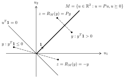
Figure 1: Illustration of the reflection operator $R_{M}$.

The iterates (8) can now be expressed as

$$\mu^{(k+1)} =J_{cT_{1}}(z^{(k)}),$$

$$y^{(k+1)} =2\mu^{(k+1)}-z^{(k)},\rule[11.38109pt]{0.0pt}{0.0pt}$$

$$z^{(k+1)} =R_{M}(y^{(k+1)}).\rule[11.38109pt]{0.0pt}{0.0pt}$$

In order to find a dual expression for $J_{cT_{1}}(z^{(k)})$, we note that

$$\tilde{\mu}=J_{cT_{1}}(z)\quad\Leftrightarrow\quad z-\tilde{\mu}\in cT_{1}(\tilde{\mu}).$$

Hence, $\tilde{\mu}=z+c(C\tilde{x}-d)$ where $\tilde{x}\in\partial f^{*}(-C^{T}\tilde{\mu})$, and thus $0\in\partial f(\tilde{x})+C^{T}\tilde{\mu}=\partial f(\tilde{x})+C^{T}z+cC^{T}(C\tilde{x}-d)$ so that

$$\tilde{x}=\arg\min_{x}\left(f(x)+z^{T}Cx+\frac{c}{2}\|Cx-d\|^{2}\right).$$

With this, the iterates can be expressed as

$$x^{(k+1)} =\displaystyle\arg\min_{x}\left(f(x)+z^{(k)\raisebox{1.99168pt}{\scriptsize$T$\!}}Cx+\frac{c}{2}\|Cx-d\|^{2}\right),$$

$$\mu^{(k+1)} =z^{(k)}+c(Cx^{(k+1)}-d),\rule[11.38109pt]{0.0pt}{0.0pt}$$

$$y^{(k+1)} =2\mu^{(k+1)}-z^{(k)},\rule[14.22636pt]{0.0pt}{0.0pt}$$

$$z^{(k+1)} =R_{M}(y^{(k+1)}),\rule[15.649pt]{0.0pt}{0.0pt}$$

which can be simplified to

$$x^{(k+1)} =\displaystyle\arg\min_{x}\left(f(x)+z^{(k)\raisebox{1.99168pt}{\scriptsize$T$\!}}Cx+\frac{c}{2}\|Cx-d\|^{2}\right),$$ (11a)

$$y^{(k+1)} =z^{(k)}+2c(Cx^{(k+1)}-d),\rule[11.38109pt]{0.0pt}{0.0pt}$$ (11b)

$$z^{(k+1)} =R_{M}(y^{(k+1)}).\rule[15.649pt]{0.0pt}{0.0pt}$$ (11c)

The iterates (11) are collectively referred to as the inequality-constraint primal-dual method of multipliers (IEQ-PDMM).

The distributed nature of PDMM can be made explicit by exploiting the structure of $C$ and $d$ and writing out the update equations (11), which is visualised in the pseudo-code of Algorithm 1. It can be seen that no direct collaboration is required between nodes during the computation of these updates, leading to an attractive (parallel) algorithm for optimisation in practical networks. The update (11c) can be interpreted as one-way transmissions of the auxiliary $y$ variables to neighbouring nodes where the actual update of the $z$ variables is done.

Algorithm 1 Synchronous IEQ-PDMM.

1:Initialise:$\quad z^{(0)}\in\mathbb{R}^{2m}$ $\triangleright$ Initialisation

2:for $k=0,...,$ do

3:     for $i\in\cal V$ do$\triangleright$ Node updates

4:         $\displaystyle x_{i}^{(k+1)}=\arg\min_{x_{i}}\bigg{(}f_{i}(x_{i})+$

5:                     $\sum_{j\in\mathcal{N}_{i}}\!\left(z_{i|j}^{(k)\raisebox{1.99168pt}{\scriptsize$T$\!}}A_{ij}x_{i}+\frac{c}{2}\|A_{ij}x_{i}-\frac{1}{2}b_{ij}\|^{2}\right)\!\!\bigg{)}$

6:         for all $j\in\mathcal{N}_{i}$ do

7:              $y_{i|j}^{(k+1)}=z_{i|j}^{(k)}+2c\left(A_{ij}x_{i}^{(k+1)}-\frac{1}{2}b_{ij}\right)$

8:         end for

9:     end for

10:

11:     for all $i\in{\cal V},j\in{\cal N}_{i}$ do$\triangleright$ Transmit variables

12:         $\textbf{node}_{j}\leftarrow\textbf{node}_{i}(y_{i|j}^{(k+1)})$

13:     end for

14:

15:     for all $i\in{\cal V},j\in{\cal N}_{i}$ do$\triangleright$ Auxiliary updates

16:         if $y_{i|j}^{(k+1)}+y_{j|i}^{(k+1)}>0$ then

17:              $z_{i|j}^{(k+1)}=y_{j|i}^{(k+1)}$

18:         else

19:              $z_{i|j}^{(k+1)}=-y_{i|j}^{(k+1)}$

20:         end if

21:     end for

22:end for

III-A Equality and inequality constraints

As mentioned before the only difference in having equality or inequality constraints is in having a nonnegativity constraint $\lambda\succeq 0$ in the latter case, and thus in the definition of the set $M$. Hence, we can trivially extend our proposed inequality constraint algorithm to include equality constraints as well. In the case of an equality constraint, we simply ignore the thresholding and exchange the associated auxiliary variables along that edge. That is, let $\mu=(\mu^{T}_{\nu},\mu^{T}_{\lambda})^{T}$, where $\mu_{\nu}$ denote the Lagrange multipliers for the equality constraints and $\mu_{\lambda}$ the Lagrange multipliers for the inequality constraints. Then $\mu_{\lambda}\succeq 0$, while $\mu_{\nu}$ is unconstrained. Defining the auxiliary variables $y$ and $z$ in a similar way, (11c) becomes

$$z^{(k+1)}_{\nu} =Py^{(k+1)},$$

$$z^{(k+1)}_{\lambda} =R_{M}(y^{(k+1)}).$$

III-B Node constraints

In the previous sections we considered constraints of the form $A_{ij}x_{i}+A_{ji}x_{j}\preceq b_{ij}$, or $A_{ij}x_{i}+A_{ji}x_{j}=b_{ij}$ in the case of equality constraints. If we set $A_{ji}$ to be the $m_{ij}\times n_{j}$ zero matrix, we have constraints of the form $A_{ij}x_{i}\preceq b_{ij}$ or $A_{ij}x_{i}=b_{ij}$, which are node constraints; it sets constraints on the values $x_{i}$ can take on. Even though $x_{j}$ is not involved in the constraint anymore, there is still communication needed between node $i$ and node $j$ since at the formulation of the extended dual problem (5) we have introduced two auxiliary variables, $\mu_{i|j}$ and $\mu_{j|i}$, one at each node, to control the constraints between node $i$ and $j$. This was done independent of the actual value of $A_{ij}$ and $A_{ji}$. In order to guarantee convergence of the algorithm, these variables need to be updated and exchanged during the iterations. Note that it is irrelevant which of the neighbouring nodes is used to define the node constraint on node $i$. We could equally well define $A_{i\ell}x_{i}\preceq b_{i\ell}$ with $\ell\in{\cal N}_{i}$, in which case there will be communication between node $i$ and node $\ell$. To avoid such communication between nodes, we can introduce dummy nodes, one for every node that has a node constraint. Let $i^{\prime}$ denote the dummy node introduced to define the node constraint on node $i$. That is, we have $A_{ii^{\prime}}x_{i}\preceq b_{ii^{\prime}}$. Since dummy node $i^{\prime}$ is only used to communicate with node $i$, it is a fictive node and can be incorporated in node $i$, thereby avoiding any network communication for node constraints.

III-C Relation with ADMM

Consider the prototype ADMM problem given by

$$\begin{array}[]{ll}\text{minimise}&f(x)+g(u),\\ \rule[11.38109pt]{0.0pt}{0.0pt}\text{subject to}&Ax+Bu=c.\end{array}$$ (12)

Following [18], we can reformulate (2) in the form (12) by introducing auxiliary variables $u_{i|j},u_{j|i}\in{\mathbb{R}}^{m_{ij}}$ such that $u_{i|j}=A_{ij}x_{i}-\frac{1}{2}b_{ij}$ and $u_{j|i}=A_{ji}x_{j}-\frac{1}{2}b_{ij}$. Collecting all auxiliary variables $u_{i|j}$ and $u_{j|i}$ into a vector $u\in{\mathbb{R}}^{2m}$ and using the matrices $C,P$ and $d$ as defined before, the constraints of (2) are given by $u=Cx-d$ and $u+Pu\preceq 0$. Hence, (2) can be equivalently expressed as

$$\begin{array}[]{ll}\text{minimise}&f(x)+g(u)\\ \rule[11.38109pt]{0.0pt}{0.0pt}\text{subject to}&Cx-u=d,\end{array}$$

where $g(u)$ is the indicator function $I_{M^{\prime}}$ on $M^{\prime}=\{u\in{\mathbb{R}}^{2m}\,|\,u+Pu\preceq 0\}$. The dual problem is therefore given by

$$\text{minimise}\;\;f^{*}(-C^{T}\mu)+I^{*}_{M^{\prime}}(\mu)+d^{T}\mu,$$ (13)

where $\mu$, as in the PDMM case, denotes the stacked vector of dual variables $\mu_{i|j}$ and $\mu_{j|i}$ associated with the edges $(i,j)\in\cal E$. The ADMM algorithm is equivalent to applying Douglas Rachford splitting to the dual problem (13). Comparing (6) and (13), we can note that the apparent difference in the dual problems is the use of $I_{M}(\mu)$ in the case of PDMM and $I^{*}_{M^{\prime}}(\mu)$ in the case of ADMM. However, we have

$$I^{*}_{M^{\prime}}(\mu)=\sup_{u}\left(\mu^{T}u-I_{M^{\prime}}(u)\right)=\left\{\begin{array}[]{ll}0,&\mu=P\mu,\,\mu\succeq 0\\ \infty\rule[14.22636pt]{0.0pt}{0.0pt}&\text{otherwise,}\end{array}\right.$$

and thus $I^{*}_{M^{\prime}}(\mu)=I_{M}(\mu)$ and we conclude that the problems (6) and (13) are identical. As Douglas-Rachford splitting is equivalent to a half-averaged form of Peaceman-Rachford splitting, half-averaged PDMM and ADMM will give identical results.

IV Convergence of (in)equality-constraint PDMM

Let $T=C_{cT_{2}}\circ C_{cT_{1}}$. Since both $C_{cT_{2}}$ and $C_{cT_{1}}$ are nonexpansive, $T$ is nonexpansive, and the sequence generated by the Banach–Picard iteration $z^{(k+1)}=T(z^{(k)})$ may fail to produce a fixed point of $T$. A simple example of this situation is $T=-I$ and $z^{(0)}\neq 0$. One way of guaranteeing convergence is to average the operator $T$. That is, let $\alpha\in(0,1)$. Then

$$z^{(k+1)}=(1-\alpha)z^{(k)}+\alpha T(z^{(k)}).$$ (14)

The iteration (14) is called damped, averaged, or Krasnosel’skii-Mann iteration, and converges weakly to a fixed point in ${\rm fix}(T)$, the fixed point set of $T$ [31, Proposition 5.16]. Alternatively, for $\alpha=1$ (no averaging), we can put additional constraints on the objective function $f(x)$ to guarantee primal convergence; if $f$ is differentiable and $m$-strongly convex, then $x^{(k)}\rightarrow x^{*}$ [18]. Note that since $T$ is at best nonexpansive, the auxiliary variables will not converge in general. In fact, they will reach an alternating limit state, similar to what has been shown for equality constraint PDMM [18].

V Stochastic coordinate descent

In order to obtain an asynchronous (averaged) IEQ-PDMM algorithm, we will apply randomised coordinate descent to the algorithms presented in Section III.

Stochastic updates can be defined by assuming that each auxiliary variable $z_{i|j}$ can be updated based on a Bernoulli random variable $U_{i|j}\in\{0,1\}$. Collecting all random variables $U_{i|j}$ in the random vector $U\in\mathbb{R}^{2m}$, following the same ordering as the entries of $z$, let $(U^{(k)})_{k\in\mathbb{N}}$ denote an i.i.d. random process defined on a common probability space $(\Omega,{\cal A},{\cal P})$, such that $U^{(k)}:(\Omega,{\cal A})\mapsto\{0,1\}^{2m}$. Hence, $U^{(k)}(\omega)\subseteq\{0,1\}^{2m}$ indicates which entries of $z^{(k)}$ will be updated at iteration $k$. We assume that the following condition holds:

$$(\forall(i,j)\in{\cal E}_{\rm d})\quad{\cal P}(\{U_{i|j}^{(1)}=1\})>0.$$ (15)

Since $(U^{(k)})_{k\in\mathbb{N}}$ is i.i.d., (15) guarantees that at every iteration, entry $z_{i|j}^{(k)}$ has nonzero probability to be updated. With this, we define the stochastic Banach-Picard iteration [32] as

$$Z^{(k+1)}=\left(I-U^{(k+1)}\right)Z^{(k)}+U^{(k+1)}T(Z^{(k)}),$$

where $Z^{(k)}$ denotes the random variable having realisations $z^{(k)}$.

In Section III we showed that $T=C_{cT_{2}}\circ C_{cT_{1}}$ is nonexpansive. Hence, if $T$ is $\alpha$-averaged, a convergence proof is given in [33, 34], where it is shown that $Z^{(k)}-T(Z^{(k)})\to 0$ almost surely. For $\alpha=1$, in general $Z^{(k)}-T(Z^{(k)})\not\to 0$ since $T$ is at best nonexpansive. However, as shown in [32], when $f$ is differentiable and $m$-strongly convex, we do have $X^{(k)}\to x^{*}$ almost surely .

V-A Asynchronous IEQ-PDMM

In practice, synchronous algorithm operation implies the presence of a global clocking system between nodes. Clock synchronisation, however, in particular in large-scale heterogeneous sensor networks, can be cumbersome. In addition, due to the heterogeneous nature of the sensors/agents, processors that are fast either because of high computing power or because of small workload per iteration, must wait for the slower processors to finish their iteration. Asynchronous algorithms partly overcome these problems as there is much more flexibility regarding the use of the information received from other processors. Here, at each iteration, a single node, or possibly a subset of nodes chosen at random, are activated. More formally, let $(\zeta^{(k)})_{k\in\mathbb{N}}$ denote an i.i.d. random process defined on a common probability space such that $\zeta^{(k)}\subseteq 2^{\cal V}$ denotes a set of indices indicating which nodes will be updated at iteration $k$. Hence, $\zeta^{(k)}$ denotes the set of active nodes at iteration $k$. Asynchronous IEQ-PDMM can be seen as a specific case of stochastic IEQ-PDMM when we define the entries of $U^{(k)}$ as

$$(\forall i\in\zeta^{(k)})(\forall j\in{\cal N}_{i})\quad U_{j|i}^{(k)}=\left\{\begin{array}[]{ll}1&\text{if }i\in\zeta^{(k)},\\ 0&\text{otherwise}.\rule[11.38109pt]{0.0pt}{0.0pt}\end{array}\right.$$

V-B IEQ-PDMM with transmission failures

IEQ-PDMM with transmission losses can also be seen as a special case of stochastic IEQ-PDMM. Let $(\eta^{(k)})_{k\in\mathbb{N}}$ denote an i.i.d. random process defined on a common probability space such that $\eta^{(k)}\subseteq 2^{{\cal E}_{\rm d}}$ denotes a set of ordered pairs of nodes indicating which entries of $z^{(k+1)}$ will be updated at iteration $k$. Hence, $\eta^{(k)}$ denotes the set of active directed edges at iteration $k$; $(i,j)\in\eta^{(k)}$ implies that there has been a successful transmission from node $i$ to node $j$, but we could have a transmission failure from node $j$ to $i$. IEQ-PDMM with transmission losses can thus be seen as a specific case of stochastic IEQ-PDMM when we define the entries of $U^{(k)}$ as

$$(\forall(i,j)\in{\cal E}_{\rm d})\quad U_{j|i}^{(k)}=\left\{\begin{array}[]{ll}1&\text{if }(i,j)\in\eta^{(k)},\\ 0&\text{otherwise}.\rule[11.38109pt]{0.0pt}{0.0pt}\end{array}\right.$$

Obviously, a combination of asynchronous updating and transmission loss can be modelled by defining

$$(\forall(i,j)\in{\cal E}_{\rm d})\quad U_{j|i}^{(k)}=\left\{\begin{array}[]{ll}1&\text{if }i\in\zeta^{(k)}\text{ and }(i,j)\in\eta^{(k)},\\ 0&\text{otherwise}.\rule[11.38109pt]{0.0pt}{0.0pt}\end{array}\right.$$

The pseudocode for lossy asynchronous IEQ-PDMM is given in Algorithm 2.

Algorithm 2 Asynchronous IEQ-PDMM.

1:Initialise:$\quad z^{(0)}\in\mathbb{R}^{2m}$$\triangleright$ Initialisation

2:for $k=0,...,$ do

3:     Select a random subset of active nodes: $\zeta^{(k)}\subseteq 2^{\mathcal{V}}$

4:     Select a random subset of active directed edges: $\eta^{(k)}\in 2^{\mathcal{E}_{\rm d}}$

5:     for $i\in\zeta^{(k)}$ do$\triangleright$ Active node updates

6:         $\displaystyle x_{i}^{(k+1)}=\arg\min_{x_{i}}\bigg{(}f_{i}(x_{i})+$

7:                     $\sum_{j\in\mathcal{N}_{i}}\!\left(z_{i|j}^{(k)\raisebox{1.99168pt}{\scriptsize$T$\!}}A_{ij}x_{i}+\frac{c}{2}\|A_{ij}x_{i}-\frac{1}{2}b_{ij}\|^{2}\right)\!\!\bigg{)}$

8:         for all $j\in\mathcal{N}_{i}$ do

9:              $y_{i|j}^{(k+1)}=z_{i|j}^{(k)}+2c\left(A_{ij}x_{i}^{(k+1)}-\frac{1}{2}b_{ij}\right)$

10:         end for

11:     end for

12:

13:     for all $i\in\zeta^{(k)},j\in{\cal N}_{i}$ do$\triangleright$ Transmit variables

14:         $\textbf{node}_{j}\leftarrow\textbf{node}_{i}(y_{i|j}^{(k+1)})$

15:     end for

16:

17:     for $i\in\zeta^{(k)},j\in\mathcal{N}_{i}:(i,j)\in\eta^{(k)}$ do$\triangleright$ Auxiliary updates

18:         if $y_{i|j}^{(k+1)}+y_{j|i}^{(k+1)}>0$ then

19:              $z_{j|i}^{(k+1)}=y_{i|j}^{(k+1)}$

20:         else

21:              $z_{j|i}^{(k+1)}=-y_{j|i}^{(k+1)}$

22:         end if

23:     end for

24:end for

VI Numerical experiments

In this section we will discuss experimental results obtained by computer simulations. We will first consider an illustrative example where we show results for a quadratic problem over a graph of $n=3$ nodes, to demonstrate convergence results for synchronous and asynchronous IEQ-PDMM, and to verify the robustness against transmission failures. Secondly, we will discuss an application of network linear programming, where we collaboratively compute the intersection of convex polytopes for target localisation. Finally, we will compare the proposed algorithm with an existing (ADMM-based) algorithm and a PDMM variant where we introduced slack variables to handle the inequality constraints.

VI-A An illustrative example

In this section we consider the minimisation of a quadratic function over a graph of $n=3$ nodes as depicted in Figure 2.

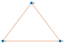
Figure 2: Graph used in the toy problem. Blue dots represent nodes whilst red lines are the edges connecting them.

We will consider the minimisation of

$$f(x)=\sum_{i\in\cal V}\frac{1}{2}(x_{i}-a_{i})^{2},$$

where $a_{i}$ is a scalar observation made at node $i$. We impose the following node constraints

$$x_{1} \geq 0,$$

$$x_{2} =1,$$

and edge constraints

$$x_{1}=x_{2},$$

$$x_{2}\geq x_{3},$$

$$x_{1}+x_{3}\leq 2.$$

Hence, we have both equality and inequality node and edge constraints. The data $a_{i}$ was randomly generated from a zero-mean unit-variance Gaussian distribution.

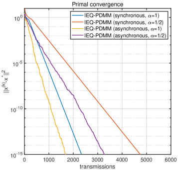
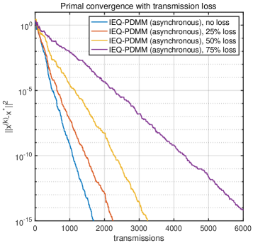
Figure 3: Convergence of IEQ-PDMM for synchronous and asynchronous update schemes with different levels of transmission loss.

Figure 3 shows convergence results for synchronous and asynchronous update schemes (left plot), where the optimal solution $x^{*}$ was computed using the MATLAB quadratic programming routine “quadprog”. In both schemes we considered non-averaged ($\alpha=1$) and averaged ($\alpha=1/2$) updates. We can observe that non-averaged updates converge in general faster than averaged updates (similar to what has been concluded for equality constraint PDMM [18]). The right plot shows convergence results in the case we have transmission losses. The latter results are only given for asynchronous IEQ-PDMM with $\alpha=1$. Hence, the blue curve in the right plot is identical to the orange curve in the left plot. We can observe that the algorithm converges for all loss rates and that the convergence rate decreases proportional to the loss rate, similar to was been observed for equality constraint PDMM [32].

VI-B Target localisation

The second simulation considers an application of network linear programming (LP) for target localisation. We consider a set of $n$ sensors randomly distributed in a unit cube which have to detect a target location $x_{\rm t}\in{\mathbb{R}}^{d}$. The sensors could be, for example, cameras, microphones or radars. We assume that each sensor has focused on the target by steering a beam towards the target, where we have added zero-mean Gaussian noise to the true direction to model uncertainty in the direction-of-arrival. We will model the beam as the intersection of a finite number of half-planes. In our two-dimensional example scenario, we will use two half-planes to model the beam pattern so that the sensing region is modeled by a cone. Figure 4 shows such a set-up, where we have four sensors indicated by the blue dots. The dashed blue lines indicate the hyperplanes (lines in ${\mathbb{R}}^{2}$) modeling the sensing beams.

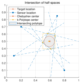
Figure 4: Target location estimation by collaboratively computing the intersection of convex polytopes.

The intersection of the regions detected by the sensors (grey area in Figure 4) can be used to estimate the target location. Since this is the intersection of half-planes, this region is a polytope which itself is convex and non-empty. The goal is to find an inner approximation of the polytope by computing the largest Euclidean ball contained in it. The centre of the optimal ball is called the Chebyshev centre of the polytope and is the point deepest inside the polytope, i.e., farthest from the boundary. A polytope, in general, can be described as

$${\cal P}=\{x\in{\mathbb{R}}^{d}:a_{\ell}^{T}x\leq b_{\ell},\,\ell=1,\ldots,m\},$$

where $m$ is the number of hyperplanes defining the polytope, and a ball as ${\cal B}=\{x_{c}+u:\|u\|<r\}$, where $x_{c}\in{\mathbb{R}}^{d}$ is the centre and $r\in{\mathbb{R}}$ the radius of the ball. Our task is to maximise $r$ subject to the constraint ${\cal B}\subseteq{\cal P}$. Finding the Chebyshev centre can be determined by solving the LP [35]

$$\begin{array}[]{ll}\text{maximise}&r,\\ \rule[11.38109pt]{0.0pt}{0.0pt}\text{subject to}&a_{\ell}^{T}x_{c}+r\|a_{\ell}\|\leq b_{\ell},\;\ell=1,\ldots,m.\end{array}$$

In order to solve this problem distributed, we introduce local variables $x_{i}$ and $r_{i}$ at each node and add the additional constraint that $x_{i}=x_{j}$ and $r_{i}=r_{j}$ for all $(i,j)\in{\cal E}$, where ${\cal E}$ is the set of edges (communication links) in the network. That is, we solve the LP

$$\begin{array}[]{ll}\text{maximise}&\displaystyle\sum_{i=1}^{n}r_{i},\\ \rule[11.38109pt]{0.0pt}{0.0pt}\text{subject to}&a_{\ell}^{T}x_{i}+r_{i}\|a_{\ell}\|\leq b_{\ell},\;\ell=1,\ldots,m,\\ \rule[11.38109pt]{0.0pt}{0.0pt}&x_{i}=x_{j},r_{i}=r_{j},\;(i,j)\in{\cal E}.\end{array}$$ (16)

Obviously, (16) is of the form of our prototypical problem with both linear equality and inequality constraints and can, therefore, be solved using IEQ-PDMM. Figure 4 shows the result (red circle and red triangle) for our two-dimensional example in the case of synchronous IEQ-PDMM. Figure 5 shows convergence results for finding the Chebyshev centre. In this example, we half-averaged the operator $T$ since the objective function is not strongly convex and the algorithm would fail to converge without averaging.

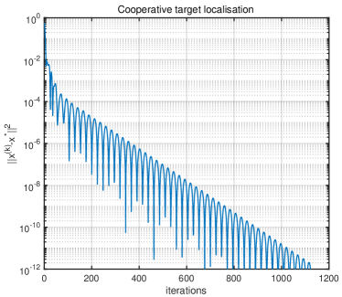
Figure 5: Convergence results for finding the Chebyshev centre.

Alternatively, we could find an outer approximation of the polytope by finding the smallest bounding rectangle (or $k$-polytope) enclosing it. In the case of a bounding rectangle, we need to solve four linear programs. Let $d_{k},k=1,\ldots,4$, denote the normal vector to the $k$th hyperplane defining the bounding rectangle. We then have to solve the following LPs:

$$\begin{array}[]{ll}\text{minimise}&d_{k}^{T}x,\\ \rule[11.38109pt]{0.0pt}{0.0pt}\text{subject to}&a_{\ell}^{T}x\leq b_{\ell},\;\ell=1,\ldots,m,\end{array}$$

for $k=1,\ldots,4$. Again, in order to solver this problem distributed, we introduce local variables $x_{i}$ at each node and add the additional constraint that $x_{i}=x_{j}$ for all $(i,j)\in{\cal E}$. That is, we solve the LPs

$$\begin{array}[]{ll}\text{minimise}&d_{k}^{T}x_{i},\\ \rule[11.38109pt]{0.0pt}{0.0pt}\text{subject to}&a_{\ell}^{T}x_{i}\leq b_{\ell},\;\ell=1,\ldots,m,\\ \rule[11.38109pt]{0.0pt}{0.0pt}&x_{i}=x_{j},\;(i,j)\in{\cal E},\end{array}$$

which are of the standard form suitable to be solved using IEQ-PDMM. The result is shown in Figure 4 (orange rectangle and corresponding centre point), where we again half-averaged the operator $T$ for the same reason as mentioned above.

VI-C Comparison with existing algorithms

In this section we consider a distributed quadratic optimisation problem with inequality constraints over a random geometric graph of $n=50$ nodes where we have set the communication radius $r=\sqrt{2\log(n)/n}$, thereby guaranteeing a connected graph with probability at least $1-1/n^{2}$ [36]. The resulting graph is depicted in Figure 6. The problem we consider here is given by

$$\begin{array}[]{ll}\text{minimise}&{\displaystyle\sum_{i\in{\cal V}}\frac{1}{2}(x_{i}-a_{i})^{2}}\\ \rule[11.38109pt]{0.0pt}{0.0pt}\text{subject to}&x_{i}\leq x_{j}\textrm{ for }i<j,\quad\;\;(i,j)\in\cal E,\end{array}$$ (17)

where the data $a_{i}$ was randomly generated from a Gaussian distribution.

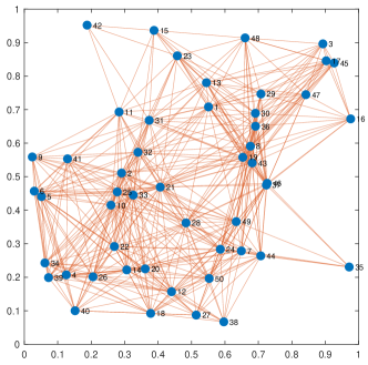
Figure 6: Demonstration of a random geometric graph with 50 nodes.

We compared three methods. First of all we compared the proposed IEQ-PDMM method with a PDMM variant where we introduced, as is commonly done, additional slack variables. The reason for this comparison is to find out if the introduction of slack variables helps accelerating the convergence. For every edge constraint we introduce a slack variable $w_{ij}\geq 0$ such that the inequality constraints in (1) can be expressed as

$$A_{ij}x_{i}+A_{ji}x_{j}+w_{ij}=b_{ij},$$

$$w_{ij}\geq 0.$$

Since standard PDMM can only handle equality constraints, the inequality constraints $w_{ij}\geq 0$ can be included in the objective function by introducing the indicator function $I_{\{w\succeq 0\}}$. However, by doing so, the objective function is not separable anymore. This can be easily overcome by introducing two slack variables per edge, $w_{i|j}\geq 0$ and $w_{j|i}\geq 0$, and add the additional equality constraint $w_{i|j}=w_{j|i}$. With this, the PDMM variant that can handle inequality constraints becomes

$$\begin{array}[]{ll}\text{minimise}&{\displaystyle\sum_{i\in{\cal V}}\left(f_{i}(x_{i})+\sum_{j\in{\cal N}_{i}}{I}_{\{w_{i|j}\geq 0\}}\right)}\\ \text{subject to}&A_{ij}x_{i}+A_{ji}x_{j}+w_{i|j}+w_{j|i}=b_{ij}\rule[11.38109pt]{0.0pt}{0.0pt}\\ &w_{i|j}-w_{j|i}=0\rule[11.38109pt]{0.0pt}{0.0pt}\hskip 85.35826pt\;\;\raisebox{6.99997pt}{$(i,j)\in\cal E$.}\end{array}$$

We will refer to this algorithm as PDMM-slack. Secondly, we will compare our proposed algorithm to a state-of-the-art ADMM-based algorithm that avoids slack variables, referred to as extended ADMM [29]. Since the extended ADMM algorithm is a synchronous update scheme, we only compare synchronous versions of the algorithms. In both IEQ-PDMM and PDMM-slack, the parameter $c$ (see Algorithm 1) was set to $c=0.5$. The two hyper-parameters $\nu$ and $\beta$ in extended ADMM [29] were searched from the discrete set $\{0.1,0.2,\ldots,1.0\}$ to produce the fastest convergence speed. The optimal setup after searching is $(\nu^{\ast},\beta^{\ast})=(0.4,0.3)$. To make a fair comparison between the methods, we set the averaging parameter $\alpha$ in (14) to $\alpha=0.5$ (ADMM). For completeness, we included results for $\alpha=1$ as well.

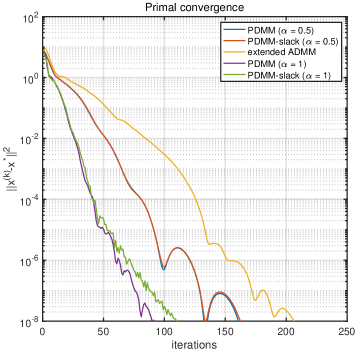
Figure 7: Convergence comparison of PDMM, PDMM-slack, and extended ADMM over the random geometric graph depicted in Figure 6.

Figure 7 visualises the convergence results of the three methods. As can be seen, both PDMM algorithms have similar convergence rates and outperform the extended ADMM algorithm in terms of number of iterations needed to converge to a certain accuracy level. However, the computational complexity of the proposed IEQ-PDMM algorithm is significantly lower than the PDMM-slack and extended ADMM algorithm. This can be seen from Table I which shows the average time (in seconds) needed per iteration for the three methods. Clearly, IEQ-PDMM consumes the least amount of time, demonstrating its efficiency. The PDMM-slack algorithm is most expensive because we have to perform an inequality constraint optimisation problem at each and every iteration (here implemented using the MATLAB program “quadprog”). The above results indicate that the introduction of slack variables does not improve the convergence rate of PDMM and that it is most efficient to handle the inequality constraints directly by imposing non-negativity constraints on the dual variables as is done in (3).

TABLE I: Comparison of computational complexity per iteration (in seconds)

IEQ-PDMM	PDMM-slack	extended ADMM [29]
0.0032	0.2076	0.0479

VII Conclusions

In this paper we have presented a node-based distributed optimisation algorithm for optimising a separable convex cost function with linear equality and ineqaulity node and edge constraints, termed inequality-constraint primal-dual method of multipliers (IEQ-PDMM). Using monotone operator theory and operator splitting, we derived node-based update rules for solving the problem. To incorporate the inequality constraints, we imposed non-negativity constraints on the associated dual variables, resulting in the introduction of a reflection operator to model the data exchange in the network, instead of a permutation operator as derived for equality constraint PDMM. We showed how to avoid unnecessary communication between nodes in the case we have node constraints by introducing fictive nodes in the network and highlighted the relation with Peaceman-Rachford splitting and ADMM. We showed convergence results for both synchronous and stochastic update schemes, where the latter includes asynchronous update schemes and update schemes with transmission losses. The algorithm converges for any CCP cost function when using averaged iterations, and has primal convergence for non-averaged updates in the case the cost function is differentiable and $m$-strongly convex.

References

- [1] S. Boyd, N. Parikh, E. Chu, B. Peleato, and J. Eckstein, “Distributed Optimization and Statistical Learning via the Alternating Direction Method of Multipliers,” In Foundations and Trends® in Machine Learning, vol. 3, no. 1, pp. 1–122, 2011.
- [2] A. G. Dimakis, S. Kar, J. M. F. Moura, M. G. Rabbat, and A. Scaglione, “Gossip Algorithms for Distributed Signal Processing,” Proceedings of the IEEE, vol. 98, no. 11, pp. 1847–1864, 2010.
- [3] T. Li, A. K. Sahu, A. Talwalkar, and V. Smith, “Federated Learning: Challenges, Methods and Future Directions,” Technical Report, arxiv.org/abs/1908.07873, 2019.
- [4] S. Boyd, A. Ghosh, B. Prabhakar, and D. Shah, “Randomized Gossip Algorithms,” IEEE Trans. Information Theory, vol. 52, no. 6, pp. 2508–2530, 2006.
- [5] D. Üstebay, B. Oreshkin, M. Coates, and M. Rabbat, “Greedy gossip with eavesdropping,” IEEE Trans. on Signal Processing, vol. 58, no. 7, pp. 3765–3776, July 2010.
- [6] F. Bénézit, A. Dimakis, P. Thiran, and M. Vetterli, “Order-optimal consensus through randomized path averaging,” IEEE Trans. on Information Theory, vol. 56, no. 10, pp. 5150–5167, October 2010.
- [7] F. Lutzeler, P. Ciblat, and W. Hachem, “Analysis of Sum-Weight-Like Algorithms for Averaging in Wireless Sensor Networks,” IEEE Trans. Signal Processing, vol. 61, no. 11, pp. 2802–2814, 2013.
- [8] M. Wainwright, T. Jaakkola, and A. Willsky, “MAP estimation via agreement on trees: Message-passing and linear programming,” IEEE Trans. Information Theory, vol. 51, no. 11, pp. 3697–3717, November 2005.
- [9] A. Schwing, T. Hazan, M. Pollefeys, and R. Urtasun, “Distributed message passing for large scale graphical models,” Proc. IEEE Conf. Comput.Vision Pattern Recognition, p. 1833–1840, 2011.
- [10] D. Shuman, S. Narang, P. Frossard, A. Ortega, and P. Vandergheynst, “The emerging field of signal processing on graphs: Extending high- dimensional data analysis to networks and other irregular domains,” IEEE Signal Process. Magazine, vol. 30, no. 3, pp. 83–98,, May 2013.
- [11] A. Loukas, A. Simonetto, and G. Leus, “Distributed autoregressive moving average graph filters,” IEEE Signal Process. Letters, vol. 22, no. 11, p. 1931–1935, Nov. 2015.
- [12] E. Isufi, A. Simonetto, A. Loukas, and G. Leus, “Stochastic graph filtering on time-varying graphs,” Proc. IEEE 6th Int. Workshop Comput. Adv. Multi-Sensor Adaptive Process., p. 89–92, 2015.
- [13] R. Xin and U. A. Khan, “A linear Algorithm for optimisation over directed graphs with geometric convergence,” IEEE Control Systems Letters, vol. 2, no. 3, pp. 315–320, 2018.
- [14] H. Yuan and T. Ma, “Federated Accelerated Stochastic Gradient Descent,” in NIPS), 2020.
- [15] S. P. Karimireddy, S. Kale, S. J. Reddi, S. U. Stich, and A. T. Suresh, “SCAFFOLD: Stochastic Controlled Averaging for Federated Learning,” in ICML, 2020.
- [16] Z. Luo and W. Yu, “An introduction to convex optimization for communications and signal processing,” IEEE Journal on Selected Areas in Communications, vol. 24, no. 8, p. 1426–1438, Aug. 2006.
- [17] G. Zhang and R. Heusdens, “Distributed Optimization using the Primal-Dual Method of Multipliers,” IEEE Trans. Signal and Information Processing over Networks, 2017.
- [18] T. W. Sherson, R. Heusdens, and W. B. Kleijn, “Derivation and analysis of the primal-dual method of multipliers based on monotone operator theory,” IEEE Transactions on Signal and Information Processing over Networks, vol. 5, no. 2, pp. 334–347, 2019.
- [19] S. O. Jordan, T. W. Sherson, and R. Heusdens, “Convergence of Stochastic PDMM,” in ICASSP, 2023.
- [20] G. Zhang, N. Kenta, and W. B. Kleijn, “Revisiting the Primal-Dual Method of Multipliers for Optimisation Over Centralised Networks,” IEEE Trans. Signal and Information Processing over Networks, vol. 8, pp. 228–243, 2022.
- [21] R. Pathak and M. J. Wainwright, “FedSplit: An algorithmic framework for fast federated optimization,” in NIPS, 2020.
- [22] Q. Li, R. Heusdens and M. G. Christensen, “Convex optimisation-based privacy-preserving distributed average consensus in wireless sensor networks,” in Proc. Int. Conf. Acoust., Speech, Signal Process., pp. 5895-5899, 2020.
- [23] Q. Li, J. S. Gundersen, R. Heusdens and M. G. Christensen, “Privacy-preserving distributed processing: Metrics, bounds, and algorithms,” in IEEE Trans. Inf. Forensics Security. vol. 16, pp. 2090–2103, 2021.
- [24] Q. Li, R. Heusdens and M. G. Christensen, “Privacy-preserving distributed optimization via subspace perturbation: A general framework,” in IEEE Trans. Signal Process., vol. 68, pp. 5983 - 5996, 2020.
- [25] J. A. G. Jonkman, T. Sherson, and R. Heusdens, “Quantisation effects in distributed optimisation,” in Proc. Int. Conf. Acoust., Speech, Signal Process., pp. 3649–3653, 2018.
- [26] C. Xu, “Generalized Lasso Problem With Equality And Inequality Constraints Using ADMM,” Ph.D. dissertation, Auburn University, 2019.
- [27] J. Giesen and S. Laue, “Combining ADMM and the Augmented Lagrangian Method for Efficiently Handling Many Constraints,” in Proceedings of the Twenty-Eighth International Joint Conference on Artificial Intelligence (IJCAI-19), 2019.
- [28] Y. Chen, M. Santillo, M. Jankovic, and A. D. Ames, “Online decentralized decision making with inequality constraints: an ADMM approach,” in IEEE Control Systems Letters, 2020.
- [29] B. He, S. Xu, and X. Yuan, “Extensions of ADMM for separable convex optimization problems with linear equality or inequality constraints,” Handbook of Numerical Analysis, vol. 24, pp. 511–557, 2023.
- [30] Y. Sawaragi, H. Nakayama, and T. Tanino, Theory of Multiobjective Optimization. Elsevier Science, 1985.
- [31] H. H. Bauschke and P. L. Combettes, Convex Analysis and Monotone Operator Theory in Hilbert Spaces, 2nd ed. Springer, 2017, cMS Books in Mathematics.
- [32] S. O. Jordan, T. W. Sherson, and R. Heusdens, “Convergence of stochastic pdmm,” in Proceedings IEEE International Conference on Acoustics, Speech and Signal Processing (ICASSP), 2023, pp. 1–5.
- [33] F. Iutzeler, P. Bianchi, P. Ciblat, and W. Hachem, “Asynchronous distributed optimizationusing a randomized alternating direction method of multipliers,” 52nd IEEE Conference on Decision and Control, pp. 3671–3676, 2013, firenze, Italy.
- [34] P. Bianchi, W. Hachem, and F. Iutzeler, “A coordinate descent primal-dual algorithmand application to distributedasynchronous optimization,” IEEE Trans. on Automatic Control, vol. 61, no. 10, pp. 2947–2957, October 2016.
- [35] S. Boyd and L. Vandenberghe, Convex Optimization. Cambridge University Press, 2004.
- [36] J. Dall and M. Christensen, “Random geometric graphs,” Phys. Rev. E, vol. 66, p. 016121, Jul 2002. [Online]. Available: https://link.aps.org/doi/10.1103/PhysRevE.66.016121