Thermal modeling of subduction zones with prescribed and evolving 2D and 3D slab geometries

Abstract

The determination of the temperature in and above the slab in subduction zones, using models where the top of the slab is precisely known, is important to test hypotheses regarding the causes of arc volcanism and intermediate-depth seismicity. While 2D and 3D models can predict the thermal structure with high precision for fixed slab geometries, a number of regions are characterized by relatively large geometrical changes. Examples include the flat slab segments in South America that evolved from more steeply dipping geometries to the present day flat slab geometry. We devise, implement, and test a numerical approach to model the thermal evolution of a subduction zone with prescribed changes in slab geometry over time. Our numerical model approximates the subduction zone geometry by employing time dependent deformation of a Bézier spline which is used as the slab interface in a finite element discretization of the Stokes and heat equations. We implement the numerical model using the FEniCS open source finite element suite and describe the means by which we compute approximations of the subduction zone velocity, temperature, and pressure fields. We compute and compare the 3D time evolving numerical model with its 2D analogy at cross-sections for slabs that evolve to the present-day structure of a flat segment of the subducting Nazca plate.

Research

1 Introduction

1.1 The importance of the thermal structure of flat slab segments

Upon subduction the oceanic lithosphere warms and undergoes metamorphic phase changes which release fluids that can lead to arc volcanism and intermediate-depth seismicity. These regions have significant potential for major natural hazards that include underthrusting seismic events along the plate interface and explosive arc volcanism. The geophysical and geochemical processes that cause such hazards are strongly controlled by temperature (for a recent review see van Keken and Wilson, 2023) and it is of great interest to a broad community of Earth scientists to understand the thermal structure of subduction zones.

Of particular interest to us is the intermediate-depth and deep seismicity that occurs at depths below the brittle-ductile transition and require mechanisms other than brittle failure. Shear heating instabilities Kelemen and Hirth (2007), dehydration embrittlement Raleigh and Paterson (1965); Jung et al. (2004), and hydration-related embrittlement (e.g., Shiina et al., 2013; van Keken et al., 2012; Shirey et al., 2021) are three such mechanisms. The difference between the last two is that dehydration embrittlement would limit the seismicity to the location of metamorphic dehydration whereas hydration-related embrittlement may occur wherever fluids that have been liberated by such dehydration reactions migrate. The wide distribution of these fluids that is predicted by fluid flow modeling Wilson et al. (2014), observed at locations of intermediate-depth seismicity Shiina et al. (2013, 2017); Bloch et al. (2018), and seen in petrological studies of exhumed oceanic crust Bebout and Penniston-Dorland (2016) provides strong support for the latter hypothesis. Thermal modeling suggests intermediate-depth seismicity is limited to be above major dehydration reactions such as that of blueschist-out or antigorite-out phase boundaries van Keken et al. (2012); Wei et al. (2017); Sippl et al. (2019). Further indications of petrological controls on the locations of seismicity are provided by Abers et al. (2013) who showed that the upper plane of seismicity in cold subduction zones tends to be limited to the oceanic crust whereas the seismicity in warm subduction zones occurs in the mantle portion of the subducting slab. See van Keken and Wilson (2023) for a broader discussion of the relationship between metamorphic dehydration reactions, fluids, and intermediate-depth seismicity.

The observational evidence, combined with modeling constraints strongly suggests fluids and intermediate-depth earthquakes are related but how can this relationship be further constrained and quantified? Wagner et al. (2020) lays out an elegant motivation that a number of flat slab regions provide natural experiments to study this question. In a number of regions on Earth, such as below Southern Alaska Finzel et al. (2011), Colombia (Wagner et al., 2017), Mexico, Peru, and Chile Manea et al. (2017), subduction zones are characterized by flat slabs where upon subduction the slab top stays flat after it reaches a certain depth below the continental lithosphere over significant distances. Periods of flat slab subduction in the geological past have also been suggested to cause orogenic events and ore deposits far from paleogeographically constrained plate boundaries. These include the late Cretaceous to Paleocene Laramide orogeny (see, e.g., Fan and Carrapa, 2014; Carrapa et al., 2019) and the Mesozoic South China fold belt Li and Li (2007). It is generally understood that these slab segments form by trench rollback with the continental lithosphere overriding the slab at shallow depth causing effective flattening.

Specific modern-day flat slab regions that would allow us to further quantify the fluid-seismicity relationship include the present-day Pampean slab (beneath Chile and Argentina) and the Peruvian flat slab segment. Both likely evolved from steeper subduction to near flat subduction due to the subduction of more buoyant thickened ridges such as the Juan Fernández and Nazca Ridges Gutscher et al. (1999); Antonijevic et al. (2015); Contreras-Reyes et al. (2019). These regions are of particular interest as the intermediate-depth seismicity varies significantly along-trench. This may be caused by a variable hydration state of the incoming lithosphere and the thermal evolution of the subduction crust and mantle (see Wagner et al., 2020, for observational evidence and the development of a testable hypothesis). These locations therefore suggest at least a qualitative correlation between fluids and seismicity. In order to further test and quantify this correlation we need a good understanding of the thermal structure of the flat slab as it evolves.

Numerical modeling provides an important complement to observational studies as it can predict the subduction zone thermal structure by computing approximations of partial differential equations’ solutions that arise from the conservation principles of mass, momentum, and thermal energy. Thermal models of flat slab segments have provided insights into the thermal evolution of the slab and overriding lithosphere but have generally been predicted using 2D cross-sections (e.g., English et al., 2003; Manea and Manea, 2011; Marot et al., 2014; Axen et al., 2018; Liu et al., 2022; Currie and Copeland, 2022). The geological evolution of the South Peruvian and Pampean slabs is influenced by strong temporal changes in 3D geometry over time. This makes reliable predictions of their thermal evolution challenging as it needs to be approached with methods that can prescribe such 3D geometrical evolution in a paleogeographically consistent fashion. A few 3D model simulations exist for flat slab reconstructions Schmid et al. (2002); Liu et al. (2008) or their geodynamical evolution Jadamec et al. (2013); Jadamec and Haynie (2017); Taramón et al. (2015) that are useful for their intended comparisons with, for example, seismic tomography or plate motions. The employed numerical resolution is generally low and it is difficult to precisely determine the slab surface which makes it difficult to use these models for the prediction of the precise thermal structure of the subducting slab needed to understand the relationships between earthquake locations, slab stratigraphy, and water content. For this purpose the slab top location should be precisely known and models should have numerical grid spacings of less than a few km in the thermal boundary layers van Keken et al. (2002, 2008).

Finite element models have the particular advantage of being able to precisely prescribe model interfaces (such as the top of the slab or the Moho of the overriding plate) and to be able to use grid refinement that allows for high resolution near thermal boundary layers with coarse grids where the velocity and temperature solutions have small gradients, allowing for high precision and computational efficiency at the same time (see, e.g., Peacock and Wang, 1999; Wada and Wang, 2009; van Keken et al., 2002; Syracuse et al., 2010; van Keken et al., 2019). In this paper we will lay the computational groundwork for such high-resolution finite element models that, due to advances in computational methods and software design, can be used to study the thermal structure of subduction zones in both 2D and 3D and with time-varying geometry in a consistent fashion. This modeling approach will allow us (and other researchers) to study the relationship between intermediate-depth seismicity, mineralogy, and water content as laid out in, for example, Wagner et al. (2020). While the examples presented here are specific for models that evolve from intermediate dip to flat slab, the open-source modeling framework we present here is sufficiently general to be used for the thermal modeling of any deforming slab geometry.

1.2 Finite element modeling of subduction zones

Thermal modeling of subduction zones aids in the interpretation of the chemical and physical processes that take place in the descending slab. To study the thermal structure of present-day subduction zones with known geometry and forcing functions (such as age of the oceanic lithosphere at the trench and convergence speed), most existing 2D models (see summary in van Keken and Wilson, 2023) combine a kinematically prescribed slab (or slab surface) and a dynamic mantle wedge (in addition to a dynamic slab if only the slab surface velocity is kinematically prescribed). This approach works well for regions where the slab geometry is fixed (even if the forcing functions may change with time). The use of finite element methods also allows for the exploration of 3D geometries enabling the study of subduction obliquity, along-trench variations in slab geometry, and interactions between multiple slabs Kneller and van Keken (2012); Bengtson and van Keken (2012); Rosas et al. (2016); Wada and He (2017); Plunder et al. (2018) that can lead to complicated 3D wedge flow that regionally affect the temperature distribution in the subducting slab.

The kinematic-dynamic approach described above has significant limitations when changes in geometry occur over the lifetime of a subduction zone. This occurs, for example, when slabs change from intermediate or steep dip to shallower dip or even to flat slab subduction.

The thermal structure of flat slabs has been investigated with 2D steady-state kinematic-dynamic models (e.g., Gutscher and Peacock, 2003; Manea et al., 2017) but the steady-state nature of these models may obscure important effects of the geometrical evolution of the slab. An alternative approach is to model subduction evolution with dynamical models (e.g. Gerya et al., 2009; Liu et al., 2022) but the modeled evolution may not conform closely to paleogeographic constraints and models of slab evolution. It may also be difficult to precisely trace out the subducting oceanic crust within the evolving slab. The inherent and complex 3D nature of these regions also suggests the best approach to understanding the thermal evolution is achieved in a framework that allows for 3D time-dependent modeling where both geometry and forcing functions can be described.

Developing such a framework lays forth a number of requirements which extend beyond the standard Finite Element (FE) discretization scheme. The subduction zone computational model must support: a) a flexible description of the time-dependent slab interface geometry; b) imposition of arbitrary geometry dependent boundary conditions; and c) scalable distribution of the discretized problem for solution with parallel linear algebra packages (i.e., support efficient computation of small 2D models on local machines and large 3D models on high performance computers).

To address these requirements we use the components of the FEniCS project for assembly of our FE systems Logg et al. (2012). The work presented here builds on our extensive experience using FEniCS for flexible solution of the equations governing subduction zone thermal structure and mantle dynamics. This includes the modeling of the thermal structure of the subduction slab with and without shear heating van Keken et al. (2019); Abers et al. (2020) and the role of fluid transport through the slab and mantle wedge Wilson et al. (2014, 2017); Cerpa et al. (2017). We have demonstrated the precision of the FEniCS applications by comparison to semi-analytical approaches (with comparisons, for example, to solutions from Molnar and England (1990) as in van Keken et al. (2019)), published subduction zone benchmarks van Keken et al. (2008), and intercode comparisons involving detailed reproductions of published models (e.g. Syracuse et al., 2010) that were made using fully independent finite element software such as Sepran van den Berg et al. (2015). Other useful geodynamical applications using FEniCS include studies of oceanic crust formation and recycling in mantle convection models Jones et al. (2021) and the accurate modeling of buoyancy driven flows in incompressible and slightly compressible media Sime et al. (2021, 2022).

In this paper we will use FEniCS for evolving subduction zone models where the final subduction zone geometry is defined by the approximation of a seismically determined slab surface position (see, e.g., figure 1) by a Bézier spline (B-spline). These B-splines may be manipulated such that a time evolving geometry may be defined. The specification of the B-spline further provides convenient interfacing with Computer–Aided Design (CAD) software such that 2D and 3D volumes of the domain of interest may be generated. These CAD geometries furthermore interface with mesh generators in a straightforward manner yielding the spatial tessellation of the domain necessary for discretization of the model by the FE method. The nature of the flow on the slab interface is handled by employing Nitsche’s method for the weak imposition of boundary data Nitsche (1971). This provides us with a much greater flexibility in the prescribed geometry-dependent flow direction along the slab interface. Finally, interfacing with the linear algebra solvers provided by the Portable, Extensible Toolkit for Scientific Computation (PETSc) library gives us the ability to tailor scalable solution methods for the underlying discretized FE linear system Balay et al. (2023).

In the remainder of this paper we will provide the mathematical and technical description for this new modeling approach, describe the numerical implementation, provide examples of the new approach to modeling the evolution of a flat segment loosely modeled on the Chilean/Argentinian geometry in both 2D and 3D, and provide a detailed comparison how the 3D models compares to the simplified 2D cross-sectional model to show that the 3D time-dependent evolution is important for determining the thermal structure of the subducting crust. In a future article we will use this new modeling ability to specifically test the hypotheses regarding the cause of intermediate-depth seismicity as laid out in Wagner et al. (2020).

2 Model

2.1 Time evolving domain

Let $t\in\mathcal{I}=[0,t_{\text{slab}}]$ be the time domain of the model where $t_{\text{slab}}$ is the total time for the slab surface to deform from its initial to final state. Let $\Omega(t)\subset\mathbb{R}^{\mathcal{d}}$ be the spatial domain of interest at a given time $t$, where $\mathcal{d}\in\{2,3\}$ is the spatial dimension. The domain has boundary $\partial\Omega(t)$ with outward pointing normal unit vector $\hat{\boldsymbol{n}}(t)$ and tangential unit vectors $\hat{\boldsymbol{\tau}}_{i}(t)$, $i=1,\ldots,\mathcal{d}-1$. For brevity of notation we assume that all quantities deriving from the domain are functions of time and write $\Omega=\Omega(t)$. Furthermore we uniquely define each point in $\Omega$ according to the standard Cartesian reference frame with coordinate tuples and orthogonal unit directions $\boldsymbol{x}=(x,z)$ and $(\hat{\boldsymbol{x}},\hat{\boldsymbol{z}})$ when $\mathcal{d}=2$ and $\boldsymbol{x}=(x,y,z)$ and $(\hat{\boldsymbol{x}},\hat{\boldsymbol{y}},\hat{\boldsymbol{z}})$ when $\mathcal{d}=3$. We further define the radial distance from the origin $r=\|\boldsymbol{x}\|_{2}$, the unit vector pointing in the radial direction $\hat{\boldsymbol{r}}$, and given the radius of the Earth $r_{0}$ we define the depth $d=r_{0}-r$.

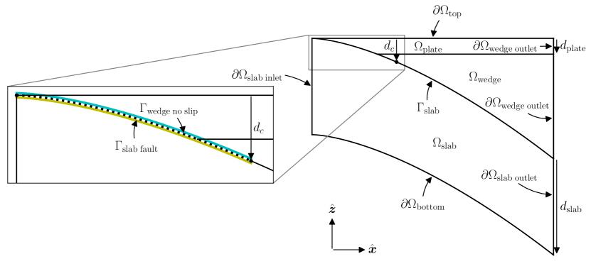
Figure 2: Schematic diagram of the subduction zone geometry employed in the model when $\mathcal{d}=2$. The inset axis highlights the subdivision of the slab interface above the coupling depth $d_{c}$. Extension to $\mathcal{d}=3$ can be envisaged as the extrusion of this geometry in the $\hat{\boldsymbol{y}}$ direction.

The exterior boundary is divided into components $\partial\Omega_{i}$ such that $\partial\Omega=\cup_{i}\partial\Omega_{i}$ and no component overlaps $\cap_{i}\partial\Omega_{i}=\emptyset$. On the interior of the geometry we prescribe an interior boundary, $\Gamma_{\text{slab}}$, with unit normal $\hat{\boldsymbol{n}}_{\text{slab}}$. This interior boundary aligns with an approximation of the subduction zone’s slab interface geometry. This interface defines the surface of bisection of the domain $\Omega$ into $\Omega_{\text{slab}}$ and $\Omega_{\text{wedge}}\cup\Omega_{\text{plate}}$ such that $\Omega=\Omega_{\text{slab}}\cup\Omega_{\text{wedge}}\cup\Omega_{\text{plate}}$ (see figure 2). $\Omega_{\text{slab}}$ extends a depth $d_{\text{slab}}$ beneath $\Gamma_{\text{slab}}$ while $\Omega_{\text{plate}}$ occupies a thickness of $d_{\text{plate}}$ at the top of the domain and above $\Gamma_{\text{slab}}$. Each of these subdomains has boundary with outward pointing unit normal vector $\hat{\boldsymbol{n}}_{\text{slab}}$, $\hat{\boldsymbol{n}}_{\text{wedge}}$ and $\hat{\boldsymbol{n}}_{\text{plate}}$, respectively.

The interior boundary $\Gamma_{\text{slab}}$ is further subdivided into components above a coupling depth, $d_{c}$, which is embedded in $\Gamma_{\text{slab}}$ (a point when $\mathcal{d}=2$ or a curve when $\mathcal{d}=3$). This coupling depth is the component of $\Gamma_{\text{slab}}$ below which the slab and wedge velocities will become fully coupled, and above which a fault discontinuity will be modeled. To facilitate this the slab and wedge domains are separated above $d_{c}$ such that the slab interface is labeled $\Gamma_{\text{slab fault}}$ from the slab side and $\Gamma_{\text{wedge no slip}}$ from the wedge side. The specific boundary conditions to be applied on each of these components will be introduced in section 2.3. A schematic diagram of an abstract representation of the $\mathcal{d}=2$ subduction zone domain is shown in figure 2. The extrusion of the shown domain in the $\hat{\boldsymbol{y}}$ direction yields a $\mathcal{d}=3$ subduction zone domain. In this case we label the near and far faces $\partial\Omega_{\text{near}}$ and $\partial\Omega_{\text{far}}$, respectively.

2.2 Underlying Partial Differential Equations (PDEs)

Quantity	Symbol	Values, reference values and/or SI units
Velocity	$\boldsymbol{u}$	$u_{\text{conv}}=$5\text{\,}\mathrm{cm}\text{\,}{\mathrm{yr}}^{-1}$$
Dynamic pressure	$p$	$\mathrm{Pa}$
Temperature	$T$	$T_{0}=$273\text{\,}\mathrm{K}$$, $T_{\text{max}}=$1573\text{\,}\mathrm{K}$$
Time	$t$	$t_{\text{slab}}=$11\text{\,}\mathrm{Myr}$$
Position	$\boldsymbol{x}$	$\mathrm{km}$
Radial distance	$r$	$r=\|\boldsymbol{x}\|_{2}$
Radius of the Earth	$r_{0}$	$6371\text{\,}\mathrm{km}$
Depth	$d$	$d=r_{0}-r$
Plate depth	$d_{\text{plate}}$	$50\text{\,}\mathrm{km}$
Coupling depth	$d_{c}$	$75\text{\,}\mathrm{km}$
Slab thickness	$d_{\text{slab}}$	$200\text{\,}\mathrm{km}$
Dynamic viscosity	$\eta$	$\mathrm{Pa}\text{\,}\mathrm{s}$ (equation 5)
Stress tensor	$\sigma$	$\mathrm{Pa}$
Density	$\rho$	$\begin{cases}$2700\text{\,}\mathrm{kg}\text{\,}{\mathrm{m}}^{-3}$&\boldsymbol{x}\in\overline{\Omega}_{\text{plate}}\text{ and }$0\text{\,}\mathrm{km}$\leq d<$40\text{\,}\mathrm{km}$\\ $3300\text{\,}\mathrm{kg}\text{\,}{\mathrm{m}}^{-3}$&\text{otherwise}\end{cases}$
Thermal conductivity	$k$	$\begin{cases}$2.5\text{\,}\mathrm{W}\text{\,}{\mathrm{m}}^{-1}\text{\,}{\mathrm{K}}^{-1}$&\boldsymbol{x}\in\overline{\Omega}_{\text{plate}}\text{ and }$0\text{\,}\mathrm{km}$\leq d<$40\text{\,}\mathrm{km}$\\ $3\text{\,}\mathrm{W}\text{\,}{\mathrm{m}}^{-1}\text{\,}{\mathrm{K}}^{-1}$&\text{otherwise}\end{cases}$
Heat capacity	$c_{p}$	$1250\text{\,}\mathrm{J}\text{\,}{\mathrm{kg}}^{-1}\text{\,}{\mathrm{K}}^{-1}$
Radiogenic heat source	$Q$	$\begin{cases}$1.3\text{\,}\mathrm{\SIUnitSymbolMicro W}\text{\,}{\mathrm{m}}^{-3}$&\boldsymbol{x}\in\overline{\Omega}_{\text{plate}}\text{ and }$0\text{\,}\mathrm{km}$\leq d<$15\text{\,}\mathrm{km}$\\ $0.27\text{\,}\mathrm{\SIUnitSymbolMicro W}\text{\,}{\mathrm{m}}^{-3}$&\boldsymbol{x}\in\overline{\Omega}_{\text{plate}}\text{ and }$15\text{\,}\mathrm{km}$\leq d\leq$40\text{\,}\mathrm{km}$\\ $0$&\text{otherwise}\\ \end{cases}$
Surface heat flux	$q_{\text{surf}}$	$65\text{\,}\mathrm{mW}\text{\,}{\mathrm{m}}^{-2}$

Table 1: Summary of physical quantities and reference values used in the model.

The subduction zone evolution is modeled by the incompressible approximation where we seek velocity $\boldsymbol{u}\mathrel{\mathop{\ordinarycolon}}\Omega\rightarrow\mathbb{R}^{\mathcal{d}}$, pressure $p\mathrel{\mathop{\ordinarycolon}}\Omega\rightarrow\mathbb{R}$ and temperature $T\mathrel{\mathop{\ordinarycolon}}\Omega\rightarrow\mathbb{R}$ which satisfy

$$-\nabla\cdot\sigma =\boldsymbol{0},$$ (1)

$$\nabla\cdot\boldsymbol{u} =0,$$ (2)

$$\rho c_{p}\mathinner{\left(\mathinner{\dfrac{\partial{}T}{\partial{t}}}+\boldsymbol{u}\cdot\nabla T\right)}-\nabla\cdot(k\nabla T) =Q,$$ (3)

with a stress tensor

$$\sigma=\eta\mathinner{\left(\nabla\boldsymbol{u}+\nabla\boldsymbol{u}^{\top}\right)}-p\boldsymbol{I}.$$ (4)

Here $\rho$ is the density, $c_{p}$ is the heat capacity, and $k$ is the thermal conductivity, which are all considered piecewise constant across the domain. $\boldsymbol{I}\in\mathbb{R}^{\mathcal{d}\times\mathcal{d}}$ is the identity tensor, $\eta\mathrel{\mathop{\ordinarycolon}}\Omega\rightarrow\mathbb{R}^{+}$ is the viscosity, and $Q\mathrel{\mathop{\ordinarycolon}}\Omega\rightarrow\mathbb{R}^{+}\cup\{0\}$ is the volumetric heat production rate. Equations 1 and 2 comprise the Stokes system of equations conserving momentum and mass, respectively. Equation 3 expresses the conservation of energy of the system under our incompressible approximation. In our numerical simulations we solve a rescaled formulation of equations 1, 2 and 3 as described in appendix A.

The viscosity model employed is that of diffusion creep combined with a near-rigid crust modeled by high viscosity such that

$$\eta(\boldsymbol{x},T)=\begin{cases}\min\mathinner{\left(\eta_{\text{max}},A_{\text{diff}}\exp\mathinner{\left(\frac{E_{\text{diff}}}{RT}\right)}\right)}&\boldsymbol{x}\in\Omega_{\text{slab}}\cup\Omega_{\text{wedge}},\\ ${10}^{5}$\eta_{\text{max}}&\boldsymbol{x}\in\Omega_{\text{plate}}.\end{cases}$$ (5)

Here $A_{\text{diff}}=$1.320\,43\text{\times}{10}^{9}\text{\,}\mathrm{Pa}\text{\,}\mathrm{s}$$ is a constant prefactor, $E_{\text{diff}}=$335\text{\times}{10}^{3}\text{\,}\mathrm{kJ}\text{\,}{\mathrm{mol}}^{-1}$$ is the activation energy, $R=$8.3145\text{\,}\mathrm{J}\text{\,}{\mathrm{mol}}^{-1}\text{\,}{\mathrm{K}}^{-1}$$ is the gas constant and $\eta_{\text{max}}=${10}^{26}\text{\,}\mathrm{Pa}\text{\,}\mathrm{s}$$ is the maximum viscosity within $\Omega_{\text{slab}}$ and $\Omega_{\text{wedge}}$. We are limiting ourselves to this temperature-dependent rheology that is based on diffusion creep in olivine Karato and Wu (1993). Detailed comparisons have shown that the near-steady state thermal structure is very similar to that when olivine dislocation creep rheology is used van Keken et al. (2008).

2.3 Boundary conditions

Description	Condition	Location
Velocity
Free slip	$\boldsymbol{u}\cdot\hat{\boldsymbol{n}}=0$ and $(\sigma\cdot\hat{\boldsymbol{n}})\cdot\hat{\boldsymbol{\tau}}_{i}=\boldsymbol{0}$, $i=1,\ldots,\mathcal{d}-1$	$\partial\Omega_{\text{top}}\cup\partial\Omega_{\text{near}}\cup\partial\Omega_{\text{far}}\cup\partial\Omega_{\text{bottom}}$
Natural in/outlet	$\sigma\cdot\hat{\boldsymbol{n}}=\boldsymbol{0}$	$\partial\Omega_{\text{slab inlet}}\cup\partial\Omega_{\text{slab outlet}}\cup\partial\Omega_{\text{wedge outlet}}$
Velocity coupled driven slab	$\boldsymbol{u}=u_{\text{conv}}\hat{\boldsymbol{\tau}}_{\text{conv}}+\boldsymbol{u}_{\text{slab}}$	$\Gamma_{\text{slab}}\cup\Gamma_{\text{slab fault}}$
Fault zone no slip	$\boldsymbol{u}=\boldsymbol{u}_{\text{slab}}$	$\Gamma_{\text{wedge no slip}}$
Temperature
Surface temperature	$T=T_{0}$	$\partial\Omega_{\text{top}}$
Inlet slab temperature	$T=T_{\text{in}}$	$\partial\Omega_{\text{slab inlet}}$
Outlet temperature influx	$T=T_{\text{out}}$	$\partial\Omega_{\text{wedge outlet}}\cup\partial\Omega_{\text{slab outlet}}$ where $\boldsymbol{u}\cdot\hat{\boldsymbol{n}}<0$
Outlet temperature outflux	$k\nabla T\cdot\hat{\boldsymbol{n}}=0$	$\partial\Omega_{\text{wedge outlet}}\cup\partial\Omega_{\text{slab outlet}}$ where $\boldsymbol{u}\cdot\hat{\boldsymbol{n}}\geq 0$
Zero heat flux	$k\nabla T\cdot\hat{\boldsymbol{n}}=0$	$\partial\Omega_{\text{near}}\cup\partial\Omega_{\text{far}}\cup\partial\Omega_{\text{bottom}}$
Temperature coupling	$T_{\text{slab}}\hat{\boldsymbol{n}}_{\text{slab}}=-T_{\text{plate}}\hat{\boldsymbol{n}}_{\text{plate}}$ and $T_{\text{slab}}\hat{\boldsymbol{n}}_{\text{slab}}=-T_{\text{wedge}}\hat{\boldsymbol{n}}_{\text{wedge}}$	$\Gamma_{\text{slab}}\cup\Gamma_{\text{wedge no slip}}\cup\Gamma_{\text{slab fault}}$

Table 2: Boundary conditions imposed in the subduction zone model domain. See section 2.3 regarding specific choices of the functions to impose.

The domain boundary $\partial\Omega$ is subdivided into components as shown in figure 2 (plus $\partial\Omega_{\text{near}}$ and $\partial\Omega_{\text{far}}$ when $\mathcal{d}=3$). The conditions to be imposed on the velocity and temperature fields are tabulated in table 2. Here we specify the functions which are imposed.

2.3.1 Slab convergence and deformation direction

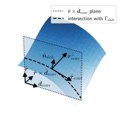
Figure 3: Schematic of the slab convergence direction. The surface $\Gamma_{\text{slab}}$ is colored by depth for visual aid. The plane defined by $\hat{\boldsymbol{r}}\times\hat{\boldsymbol{d}}_{\text{conv}}$ and its intersection with $\Gamma_{\text{slab}}$ are highlighted. The slab surface normal vector $\hat{\boldsymbol{n}}_{\text{slab}}$, the slab convergence direction $\hat{\boldsymbol{\tau}}_{\text{conv}}$ and the perpendicular vector $\hat{\boldsymbol{\tau}}^{\bot}_{\text{conv}}$ are drawn as arrows on the surface.

The down going slab velocity is decomposed into two components, a convergence speed $u_{\text{conv}}$ acting in the direction $\hat{\boldsymbol{\tau}}_{\text{conv}}$ and the velocity of the geometry’s time evolving deformation, $\boldsymbol{u}_{\text{slab}}$, such that $\boldsymbol{u}=u_{\text{conv}}\hat{\boldsymbol{\tau}}_{\text{conv}}+\boldsymbol{u}_{\text{slab}}$ on $\Gamma_{\text{slab}}\cup\Gamma_{\text{slab fault}}$. We define $\hat{\boldsymbol{\tau}}_{\text{conv}}$ in terms of a prescribed direction, $\hat{\boldsymbol{d}}_{\text{conv}}$. The vector $\hat{\boldsymbol{\tau}}_{\text{conv}}$ is the unit vector lying tangential to $\Gamma_{\text{slab}}$, parallel to $\hat{\boldsymbol{d}}_{\text{conv}}$ and in the direction of $\hat{\boldsymbol{d}}_{\text{conv}}$. This may also be interpreted as $\hat{\boldsymbol{\tau}}_{\text{conv}}$ is the vector pointing in direction $\hat{\boldsymbol{d}}_{\text{conv}}$ and tangential to the intersection of the surface $\Gamma_{\text{slab}}$ and the surface defined by the normal vector $\hat{\boldsymbol{r}}\times\hat{\boldsymbol{d}}_{\text{conv}}$ (see figure 3). We therefore define

$$\hat{\boldsymbol{\tau}}_{d} =\hat{\boldsymbol{n}}_{\text{slab}}\times\mathinner{\left(\hat{\boldsymbol{r}}\times\hat{\boldsymbol{d}}_{\text{conv}}\right)},$$ (6)

$$\hat{\boldsymbol{\tau}}_{\text{conv}} =\begin{cases}\hat{\boldsymbol{\tau}}_{d}&\hat{\boldsymbol{\tau}}_{d}\cdot\hat{\boldsymbol{d}}_{\text{conv}}\geq 0,\\ -\hat{\boldsymbol{\tau}}_{d}&\hat{\boldsymbol{\tau}}_{d}\cdot\hat{\boldsymbol{d}}_{\text{conv}}<0.\end{cases}$$ (7)

Furthermore we define the remaining vector lying tangential to $\Gamma_{\text{slab}}$ and perpendicular to $\hat{\boldsymbol{\tau}}_{\text{conv}}$ and $\hat{\boldsymbol{n}}_{\text{slab}}$.

$$\hat{\boldsymbol{\tau}}^{\bot}_{\text{conv}}=\hat{\boldsymbol{n}}_{\text{slab}}\times\hat{\boldsymbol{\tau}}_{\text{conv}}.$$ (8)

A schematic diagram of these vectors is shown in figure 3.

In addition to the prescribed slab convergence velocity we include the slab deformation velocity as a result of time-dependent geometry changes. We write $\boldsymbol{u}_{\text{slab}}$ and $\hat{\boldsymbol{d}}_{\text{slab}}$ to be the slab deformation velocity and direction, respectively. These quantities will be fully defined in section 3 where we will also describe the mathematical representation of $\Gamma_{\text{slab}}$.

2.3.2 Temperature models

The surface temperature is assumed to be a constant value

$$T_{0}=$273\text{\,}\mathrm{K}$.$$ (9)

The slab inlet temperature is selected from a half space cooling model

$$T_{\text{in}}=T_{0}+(T_{\text{max}}-T_{0})\operatorname*{erf}\mathinner{\left(\frac{d}{2\kappa_{\text{in}}t_{$50\text{\,}\mathrm{Myr}$}}\right)},$$ (10)

where $T_{\text{max}}=$1573\text{\,}\mathrm{K}$$ is the maximum temperature, $\operatorname*{erf}(\cdot)$ is the error function, $\kappa_{\text{in}}=\left.k/(\rho c_{p})\right|_{\boldsymbol{x}\in\partial\Omega_{\text{slab inlet}}}$ is the thermal diffusivity at the slab inlet and $t_{$50\text{\,}\mathrm{Myr}$}$ is $50\text{\,}\mathrm{Myr}$.

The outlet temperature is

$$T_{\text{out}}=\min\left\{T_{\text{1D}},T_{\text{max}}\right\},$$ (11)

where $T_{\text{1D}}(d)$ is the solution of the initial value problem

$$-\frac{\operatorname{d\!}}{\operatorname{d\!}d}\mathinner{\left(k\mathinner{\dfrac{\operatorname{d\!}{}T_{\text{1D}}}{\operatorname{d\!}{d}}}\right)}=Q,\quad T_{\text{1D}}(d=0)=T_{0},\quad\left.\mathinner{\left(k\mathinner{\dfrac{\operatorname{d\!}{}T_{\text{1D}}}{\operatorname{d\!}{d}}}\right)}\right|_{d=0}=q_{\text{surf}},$$ (12)

where $q_{\text{surf}}$ is the surface heat flux (see table 1 for values used in this work).

3 Discretization and solution

In this section we introduce the discretization and solution schemes we employ to compute numerical approximations of the evolving subduction zone model. We summarize our procedure in algorithm 1.

Obtain point clouds from assumed slab geometry (e.g. figure 1)

Transform point cloud data to Cartesian coordinates (section 3.1)

Project data to B-spline s as final surface approximation (section 3.2)

Generate sequence of domains and meshes of time evolving slab surface (sections 3.3 and 3.4)

Compute initial velocity, pressure and temperature approximation (section 3.6)

for each time step do

     Compute velocity, pressure and temperature approximation using algorithm 2 (section 3.6)

     Transfer temperature field to next mesh (section 3.5)

end for

Algorithm 1 Computational model summary.

3.1 Mapping slab surface geometries to coordinate data

Seismic readings provide observations of the slab interface geometry. These data consist of coordinate tuples of longitude, latitude and depth. Our aim is to transform these data into a Cartesian system where a central radial vector aligns with the $\hat{\boldsymbol{z}}$ direction.

Let the set of $N_{i}$ longitude $\lambda_{i}$, latitude $\mu_{i}$ and depth $d_{i}$ data points for a given point on the slab surface be

$$\Lambda_{\text{slab}}=\{\lambda_{i},\mu_{i},d_{i}\}_{i=1}^{N_{i}},$$ (13)

where longitude and latitude are measured in degrees and depth in kilometers. Initially these data are transformed to align the central radial vector with the $\hat{\boldsymbol{z}}$ axis of the Cartesian system. We define

$$\lambda_{\text{mid}}=\frac{1}{2}\mathinner{\left(\max_{i=1,\ldots,N_{i}}\lambda_{i}+\min_{i=1,\ldots,N_{i}}\lambda_{i}\right)}\text{ and }\mu_{\text{mid}}=\frac{1}{2}\mathinner{\left(\max_{i=1,\ldots,N_{i}}\mu_{i}+\min_{i=1,\ldots,N_{i}}\mu_{i}\right)}$$ (14)

such that

$$\overline{\Lambda}_{\text{slab}}=\{\lambda_{i}-\lambda_{\text{mid}},\mu_{i}-\mu_{\text{mid}},d_{i}\}_{i=1}^{N_{i}},$$ (15)

with spherical and Cartesian coordinate representations

$$\Phi_{\text{slab}}=\{r_{i},\theta_{i},\phi_{i}\}_{i=1}^{N_{i}},\quad X_{\text{slab}}=\{x_{i},y_{i},z_{i}\}_{i=1}^{N_{i}},$$ (16)

respectively. The transform to each system is given by

$$\Phi_{\text{slab}}=\begin{pmatrix}r_{i}\\ \theta_{i}\\ \phi_{i}\end{pmatrix}=\begin{pmatrix}r_{0}-d_{i}\\ \mathrm{radians}(\lambda_{i}-\lambda_{\text{mid}})\\ \mathrm{radians}(90-(\mu_{i}-\mu_{\text{mid}}))\end{pmatrix},\quad X_{\text{slab}}=\begin{pmatrix}x_{i}\\ y_{i}\\ z_{i}\end{pmatrix}=\begin{pmatrix}r_{i}\cos\theta_{i}\sin\phi_{i}\\ r_{i}\sin\theta_{i}\sin\phi_{i}\\ r_{i}\cos\phi_{i}\end{pmatrix}.$$ (17)

3.2 Surface data to B-spline approximation

We seek a smooth and continuous approximation of the slab interface surface from the seismic observation data $X_{\text{slab}}$. To this end, the data $X_{\text{slab}}$ are approximated by an $l_{2}$ projection to a non-periodic B-spline of order $\mathcal{p}$ (see, e.g., Piegl and Tiller, 1997).

We define a non-periodic B-spline by

$$S_{(\mathcal{p},\Xi)}(\xi)=\sum_{i=0}^{n}\boldsymbol{C}_{i}B_{i,\mathcal{p}}(\xi),$$ (18)

where $\mathcal{p}=m-n-1$ is the B-spline order, $\boldsymbol{C}_{i}$, $i=0,\ldots,n$, are the control points, $\Xi=\{\xi_{i}\}_{i=0}^{m}$ is the knot vector where each knot lies in the unit interval $\xi_{i}\in\mathinner{\left[0,1\right]}$, $i=0,\ldots,m$, each knot is ordered such that $\xi_{i}\leq\xi_{i+1}$, $i=0,\ldots,m-1$, and $B_{i,\mathcal{p}}(\xi)$, $i=0,\ldots,m$, are the B-spline basis functions. On the unit interval $\xi\in\mathinner{\left[0,1\right]}$ these basis functions are

$$B_{i,0}(\xi) =\begin{cases}1&\text{if }\xi_{i}\leq\xi<\xi_{i+1},\\ 0&\text{otherwise},\end{cases}$$ (19)

$$B_{i,k}(\xi) =\mathinner{\left(\frac{\xi-\xi_{i}}{\xi_{i+k}-\xi_{i}}\right)}B_{i,k-1}(\xi)+\mathinner{\left(\frac{\xi_{i+k+1}-\xi}{\xi_{i+k+1}-\xi_{i+1}}\right)}B_{i+1,k-1}(\xi),\quad k>0.$$ (20)

A B-spline surface of order $\boldsymbol{\mathcal{p}}=(\mathcal{p}_{1},\mathcal{p_{2}})$ is defined by a tensor product of B-spline s on the orthogonal coordinates $\boldsymbol{\xi}=(\xi_{1},\xi_{2})\in\mathinner{\left[0,1\right]}^{2}$ such that

$$S_{(\boldsymbol{\mathcal{p}},\boldsymbol{\Xi})}(\boldsymbol{\xi})=\sum_{i=0}^{n_{1}}\sum_{j=0}^{n_{2}}\boldsymbol{C}_{i,j}B_{i,\mathcal{p}_{1}}(\xi_{1})B_{j,\mathcal{p}_{2}}(\xi_{2}).$$ (21)

With the definition of the B-spline surface in place we define the evolution of the slab surface with time. Let $\vartheta(t)\mathrel{\mathop{\ordinarycolon}}\mathcal{I}\rightarrow\mathinner{\left[0,1\right]}$ be a parametrization of the evolution period of the slab. We write the slab surface B-spline

$$S^{\text{slab}}_{(\boldsymbol{\mathcal{p}},\boldsymbol{\Xi})}(\boldsymbol{\xi},t)=(1-\vartheta(t))S^{\text{initial}}_{(\boldsymbol{\mathcal{p}},\boldsymbol{\Xi})}(\boldsymbol{\xi})+\vartheta(t)S^{\text{final}}_{(\boldsymbol{\mathcal{p}},\boldsymbol{\Xi})}(\boldsymbol{\xi})$$ (22)

where $S^{\text{initial}}_{(\boldsymbol{\mathcal{p}},\boldsymbol{\Xi})}(\boldsymbol{\xi})$ and $S^{\text{final}}_{(\boldsymbol{\mathcal{p}},\boldsymbol{\Xi})}(\boldsymbol{\xi})$ are the initial and final slab geometries, respectively. We emphasize that $S^{\text{initial}}$ and $S^{\text{final}}$ share a common order, $\boldsymbol{\mathcal{p}}$, and knot vector, $\boldsymbol{\Xi}$. Their individual definition is determined by their distinct control points $\boldsymbol{C}^{\text{initial}}_{i,j}$ and $\boldsymbol{C}^{\text{final}}_{i,j}$.

With appropriate choices of $\vartheta(t)$ the putative evolution of the slab may be prescribed in the model. In our experiments we employ a straightforward linear transition such that

$$\vartheta(t)=\frac{t}{t_{\text{slab}}}.$$ (23)

This linear transition also favors a simple definition of the deformation path undertaken by the modeled slab surface

$$\boldsymbol{d}_{\text{slab}}=S^{\text{final}}_{(\boldsymbol{\mathcal{p}},\boldsymbol{\Xi})}(\boldsymbol{\xi})-S^{\text{initial}}_{(\boldsymbol{\mathcal{p}},\boldsymbol{\Xi})}(\boldsymbol{\xi})$$ (24)

along with the velocity of the slab deformation

$$\boldsymbol{u}_{\text{slab}}=\frac{1}{t_{\text{slab}}}\boldsymbol{d}_{\text{slab}}.$$ (25)

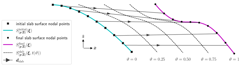
Figure 4: Schematic diagram of the slab interface geometry designed as a B-spline in physical space, $(x,z)$, evolving over parametrized time, $\vartheta$. The putative initial and observed final coordinates of points on the assumed slab surface are interpolated to splines with an equal number of control points and equal number of knot vectors yielding $\Gamma_{\text{slab}}(\vartheta=0)$ and $\Gamma_{\text{slab}}(\vartheta=1)$. The slab interface surface at intermediate time is generated according to equation 22. The displacement vector of the slab surface, $\boldsymbol{d}_{\text{slab}}$, is shown from the initial to the final configuration.

A schematic of the evolution of $S^{\text{slab}}_{(\boldsymbol{\mathcal{p}},\boldsymbol{\Xi})}$ is shown in figure 4. We highlight that this method may be extended to arbitrary numbers of prescribed initial, intermediate, and final subduction zone geometries yielding more sophisticated evolution.

3.3 Enveloping the slab surface

With the representation of the slab evolution using a B-spline we now require its envelopment in a model volume geometry as described in figure 2. A motivating advantage of a B-spline representation of $\Gamma_{\text{slab}}$ is its typical compatibility with CAD software (e.g., Open CASCADE Technology, 2022), which leverage splines to describe complicated geometries. These splines may be manipulated with a number of geometric operations, of which we employ:

• Extrusion: Transform a spline along a path generating a higher dimensional shape from the swept path.

• Union, intersection and difference: On a collection of shapes generate a single shape composed of their boolean union, intersection or difference, respectively.

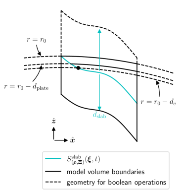
Figure 5: Schematic of the slab surface envelopment into a volume by employing spline manipulations typically offered by CAD software.

With these operations we describe the process we employ, in a qualitative sense, which provides us with the geometry volumes demonstrated in this work. A diagram of this process is shown in figure 5.

To generate the slab volume, $\Omega_{\text{slab}}$, the spline $S^{\text{slab}}_{(\boldsymbol{p},\boldsymbol{\Xi})}(\boldsymbol{\xi},t)$ is extruded in the $-\hat{\boldsymbol{z}}$ direction by a distance of $d_{\text{slab}}$. To generate the plate and wedge volumes, $\Omega_{\text{plate}}\cup\Omega_{\text{wedge}}$, the spline $S^{\text{slab}}_{(\boldsymbol{p},\boldsymbol{\Xi})}(\boldsymbol{\xi},t)$ is extruded in the $\hat{\boldsymbol{z}}$ direction by a distance greater than the maximum extent of the depth of the spline. This volume is then intersected with a sphere of radius $r_{0}$ yielding $\Omega_{\text{plate}}\cup\Omega_{\text{wedge}}$. The distinct volumes $\Omega_{\text{plate}}$ and $\Omega_{\text{wedge}}$ are then formed by embedding the surface of a sphere of radius $r_{0}-d_{\text{plate}}$. The coupling depth is also embedded in $S^{\text{slab}}_{(\boldsymbol{\mathcal{p}},\boldsymbol{\Xi})}$ by finding the intersection with a sphere of radius $r_{0}-d_{c}$.

3.4 Spatial and temporal discretization

The time interval $\mathcal{I}=\mathinner{\left[0,t_{\text{slab}}\right]}$ is discretized into time steps $\mathcal{I}_{\Delta t}=\mathinner{\left\{t_{0},t_{1},\ldots,t_{\text{slab}}\right\}}$ where $t_{0}<t_{1}<\ldots<t_{\text{slab}}$. We write the time step size $\Delta t_{n}=t_{n+1}-t_{n}$ and we use the superscript index $n$ to denote the evaluation of a function at a particular time step, e.g., $T^{n}=T(t_{n})$. At each time step, the domain $\Omega^{n}=\Omega(t_{n})$ is subdivided into a tessellation of simplices (triangles when $\mathcal{d}=2$ and tetrahedra when $\mathcal{d}=3$) which we call a mesh. Each simplex in the mesh is named a cell and denoted $\kappa$ such that the tessellation $\mathcal{T}^{n}=\{\kappa^{n}\}$. The meshing procedure accounts for the internal boundary $\Gamma_{\text{slab}}(t_{n})$ ensuring facets of cells are aligned with the surface providing an appropriate approximation.

The spatial components of equations 1, LABEL:, 2, LABEL: and 3 are discretized by the FE method. We employ a $P2$-$P1$ Taylor-Hood element pair for the Stokes system’s velocity and pressure approximations Taylor and Hood (1973) and a standard quadratic continuous Lagrange element for the temperature approximation. The boundary conditions enforced on $\Gamma_{\text{slab fault}}$ and $\Gamma_{\text{wedge no slip}}$ require a discontinuous velocity solution. Furthermore a discontinuous pressure solution is required on $\Gamma_{\text{slab fault}}$, $\Gamma_{\text{wedge no slip}}$ and $\Gamma_{\text{slab}}$. The jump conditions of the temperature approximation are satisfied by enforcing $C^{0}$ continuity across $\Gamma_{\text{slab fault}}$, $\Gamma_{\text{wedge no slip}}$ and $\Gamma_{\text{slab}}$. To this end we define the following spaces:

1. $\boldsymbol{V}^{h,n}=\{\mathcal{d}$-dimensional piecewise polynomials of degree $2$ defined in each cell of the mesh $\mathcal{T}^{n}$ and continuous across cell boundaries except those which overlap the interior boundaries $\Gamma_{\text{slab fault}}$ and $\Gamma_{\text{wedge no slip}}$ $\}$,

2. $Q^{h,n}=\{$scalar piecewise polynomials of degree $1$ defined in each cell of the mesh $\mathcal{T}^{n}$ and continuous across cell boundaries except those which overlap the interior boundaries $\Gamma_{\text{slab fault}}$, $\Gamma_{\text{wedge no slip}}$ and $\Gamma_{\text{slab}}$ $\}$,

3. $S^{h,n}=\{$scalar piecewise polynomials of degree $2$ defined in each cell of the mesh $\mathcal{T}^{n}$ and continuous across all cell boundaries$\}$.

On $\mathcal{I}_{\Delta t}$ the time derivative in the the heat equation is discretized using a finite difference scheme such that

$$\mathinner{\dfrac{\partial{}T}{\partial{t}}}\approx\frac{(T^{n+1}-T^{n})}{\Delta t_{n}}.$$ (26)

Using a backward Euler discretization allows us to write the fully discrete FE formulation for the model: find $(\boldsymbol{u}^{n+1}_{h},p^{n+1}_{h},T^{n+1}_{h})\in(\boldsymbol{V}^{h,n+1}\times Q^{h,n+1}\times S^{h,n+1})$ such that

$$\mathcal{F}^{\text{momentum}}(\boldsymbol{u}^{n+1}_{h},p^{n+1}_{h},T^{n+1}_{h})=$$

$$\quad\quad(\sigma^{n+1}_{h},\nabla\boldsymbol{v}_{h})+A^{\text{momentum}}_{\partial\Omega}((\boldsymbol{u}^{n+1}_{h},p^{n+1}_{h},T^{n+1}_{h}),\boldsymbol{v}_{h})\equiv 0,$$ (27)

$$\mathcal{F}^{\text{mass}}(\boldsymbol{u}^{n+1}_{h},p^{n+1}_{h},T^{n+1}_{h})=$$

$$\quad\quad(\nabla\cdot\boldsymbol{u}^{n+1}_{h},q_{h})+A^{\text{mass}}_{\partial\Omega}((\boldsymbol{u}^{n+1}_{h},p^{n+1}_{h},T^{n+1}_{h}),q_{h})\equiv 0,$$ (28)

$$\mathcal{F}^{\text{energy}}(\boldsymbol{u}^{n+1}_{h},p^{n+1}_{h},T^{n+1}_{h})=$$

$$\quad\quad\mathinner{\left(\rho c_{p}\mathinner{\left((T^{n+1}_{h}-T^{n}_{h})/\Delta t_{n}+\boldsymbol{u}^{n+1}_{h}\cdot\nabla T^{n+1}_{h}\right)},s_{h}\right)}+(k\nabla T^{n+1}_{h},\nabla s_{h})$$

$$\quad\quad\quad\quad+A^{\text{energy}}_{\partial\Omega}((\boldsymbol{u}^{n+1}_{h},p^{n+1}_{h},T^{n+1}_{h}),s_{h})-\mathinner{\left(Q,s_{h}\right)}\equiv 0,$$ (29)

for all $(\boldsymbol{v}_{h},q_{h},s_{h})\in(\boldsymbol{V}^{h,n+1}\times Q^{h,n+1}\times S^{h,n+1})$. Here $(a,b)=\sum_{\kappa\in\mathcal{T}^{n+1}}\int_{\kappa}a\mathrel{\mathop{\ordinarycolon}}b\operatorname{d\!}\boldsymbol{x}$ is the inner product on the mesh and the terms $A^{i}_{\partial\Omega}(\cdot,\cdot)$ are the terms arising from the weak imposition of the boundary conditions via Nitsche’s method stated in section 2.3. We refer to Houston and Sime (2018) regarding the formulation of these terms. With this discretization scheme we also define the discretized slab deformation velocity component used in the velocity boundary condition

$$\boldsymbol{u}^{n+1}_{\text{slab}}(\boldsymbol{x})=\frac{1}{\Delta t_{n}}\mathinner{\left(S^{\text{slab}}_{(\boldsymbol{p},\boldsymbol{\Xi})}(\boldsymbol{\xi}(\boldsymbol{x}),t^{n+1})-S^{\text{slab}}_{(\boldsymbol{p},\boldsymbol{\Xi})}(\boldsymbol{\xi}(\boldsymbol{x}),t^{n})\right)}.$$ (30)

3.5 Nonmatching mesh interpolation

An operator $\mathcal{P}(\cdot)$ is necessary to transfer the temperature field from the previous time step, $T^{n}_{h}(\mathcal{T}^{n})$, to the mesh at the subsequent time step, $T^{n}_{h}(\mathcal{T}^{n+1})$, such that

$$T^{n}_{h}(\mathcal{T}^{n+1})=\mathcal{P}(T^{n}_{h}(\mathcal{T}^{n})).$$ (31)

The choice of $\mathcal{P}(\cdot)$ must account for cases where subsequent meshes do not overlap. In this work we design $\mathcal{P}(\cdot)$ to be a nearest-neighbor interpolation such that $\mathcal{P}(T^{n}_{h}(\mathcal{T}^{n}))$ interpolates $T^{n}_{h}(\mathcal{T}^{n})$ in the overlapping volume $\mathcal{T}^{n+1}\cap\mathcal{T}^{n}$. In the remaining volume, $\mathcal{T}^{n+1}\setminus\mathcal{T}^{n}$, $\mathcal{P}(T^{n}_{h}(\mathcal{T}^{n}))$ interpolates the value of $T^{n}_{h}(\mathcal{T}^{n})$ which lies closest to the interpolation point. Specifically for each interpolation point $\boldsymbol{x}_{i}$ of $T^{n}_{h}(\mathcal{T}^{n+1})$ we have

$$T^{n}_{h}(\mathcal{T}^{n+1})(\boldsymbol{x}_{i})=\mathcal{P}(T^{n}_{h}(\mathcal{T}^{n}))(\boldsymbol{x}_{i}) =\begin{cases}T^{n}_{h}(\mathcal{T}^{n})(\boldsymbol{x}_{i})&\forall\boldsymbol{x}_{i}\in\mathcal{T}^{n},\\ T^{n}_{h}(\mathcal{T}^{n})(\operatorname*{arg\,min}_{\boldsymbol{y}\in\mathcal{T}^{n}}(\|\boldsymbol{x}_{i}-\boldsymbol{y}\|))&\text{otherwise},\end{cases}$$

$$i =1,\ldots,\dim(S^{h,n+1}).$$ (32)

Our choice of $\mathcal{P}(\cdot)$ here is the motivation for selecting the backward Euler finite difference scheme in the temporal discretization. A higher order finite difference scheme will have to carefully account for fields defined on both $\mathcal{T}^{n+1}$ and $\mathcal{T}^{n}$ in the FE formulation.

3.6 Picard iteration and computational linear algebra solvers

The fully discrete system in equations 27, 28 and 29 is nonlinear. We use a Picard iterative scheme to compute their solutions’ approximations and minimize the residual formulations. This requires us to split the solution of the Stokes system from the energy equation. Therefore we introduce a subscript index, $\ell$, corresponding to the Picard iteration number. Given an initial guess of the temperature field $T^{n+1}_{h,\ell=0}=\mathcal{P}(T^{n}_{h})$, we compute the sequence as shown in algorithm 2.

The linear systems which underlie the FE discretization are typically too large to compute in reasonable time with direct factorization due to the spatial fidelity required from the mesh. This is especially pertinent in the $\mathcal{d}=3$ case where computation by direct factorization is unfeasible. We employ an iterative scheme for both the Stokes and heat equation sub problems in each Picard iteration. The Stokes system is solved by full Schur complement reduction using FGMRES iterative method Saad (1993). The velocity block is preconditioned using the algebraic multigrid method with near-nullspace informed smoothed aggregation as provided by PETSc Balay et al. (2019). The pressure block is preconditioned with the inverse viscosity weighted pressure mass matrix. The heat equation is solved using GMRES iterative method Saad and Schultz (1986) and preconditioned with incomplete LU (iLU) factorization. For more details on solving such systems using iterative schemes and devising appropriate preconditioners see, for example, May and Moresi (2008).

$\ell=0$

Initialize $T^{n+1}_{h,\ell=0}=\mathcal{P}(T^{n}_{h})$

do

     $\ell\leftarrow\ell+1$

     Solve for $\boldsymbol{u}^{n+1}_{h,\ell}$ and $p^{n+1}_{h,\ell}$:

          $\mathcal{F}^{\text{momentum}}(\boldsymbol{u}^{n+1}_{h,\ell},p^{n+1}_{h,\ell},T^{n+1}_{h,\ell-1})+\mathcal{F}^{\text{mass}}(\boldsymbol{u}^{n+1}_{h,\ell},p^{n+1}_{h,\ell},T^{n+1}_{h,\ell-1})=0$

     Solve for $T^{n+1}_{h,\ell}$:

          $\mathcal{F}^{\text{energy}}(\boldsymbol{u}^{n+1}_{h,\ell},p^{n+1}_{h,\ell},T^{n+1}_{h,\ell})=0$

while $\|T^{n+1}_{h,\ell}-T^{n+1}_{h,\ell-1}\|_{L_{2}}/\|T^{n+1}_{h,\ell}\|_{L_{2}}<\mathrm{TOL}$

Algorithm 2 Picard iterative scheme employed to compute the approximate solution of the nonlinear system equations 27, 28 and 29. Here $\|\cdot\|_{L_{2}}=\sqrt{(\cdot,\cdot)}$ is the $L_{2}$ norm measure and $\mathrm{TOL}\ll 1$ is the convergence threshold tolerance (selected to be $\mathrm{TOL}=${10}^{-6}$$ in this work).

4 Implementation

In this section we list the computational tools and libraries which facilitate our computational model. The FE system assembly is enabled by the FEniCS project, this includes:

1. Basix for pre-computation of FE bases Scroggs et al. (2022),

2. Unified Form Language (UFL) for the computational symbolic algebra representation of FE formulations Alnæs et al. (2014),

3. FEniCS Form Compiler (FFC) for translation to efficient FE kernels Kirby and Logg (2006),

4. DOLFINx for the data structures and algorithms necessary for computing FE functions, tabulating their degrees of freedom, managing meshes and facilitating the solution of FE linear systems by third party linear algebra packages Logg and Wells (2010).

The components of the FEniCS project have been demonstrated to be scalable in the context of thermomechanical analysis in Richardson et al. (2019), where the linear operators underlie the momentum and energy FE discretizations in this work also.

DOLFINx-MPC Dokken (2022) is used in combination with DOLFINx to construct the function spaces $\boldsymbol{V}^{h,n}$, $Q^{h,n}$ and $S^{h,n}$. Specifically DOLFINx-MPC facilitates strong imposition of equality of the FE functions’ degrees of freedom at the $\Gamma_{\text{slab}}$, $\Gamma_{\text{slab fault}}$ and $\Gamma_{\text{wedge no slip}}$ boundaries as required by the velocity and temperature boundary conditions.

The Python library NURBS-Python (geomdl) Bingol and Krishnamurthy (2019) is employed for the B-spline approximation of $\Gamma_{\text{slab}}$. Its data structures and functions are necessary for B-spline initialization and manipulation along with its facilitation of the $l_{2}$ minimization of point cloud positional data to the B-spline surface geometry.

The computational domain is defined using the CAD framework offered by Open CASCADE Technology (2022). These geometries are then interpreted by the meshing library gmsh Geuzaine and Remacle (2009) for generation of the sequence of simplicial meshes for each time step between the initial and final slab geometry configurations.

The PETSc library Balay et al. (2023, 2019) is used for its data structures and algorithms facilitating distributed parallel computation of the linear algebra systems’ solutions. This includes the implementations of the Flexible Generalized Minimal Residual (FGMRES) and Generalized Minimal Residual (GMRES) methods, along with construction of iLU factorization and construction of algebraic multigrid preconditioners.

Automatic formulation of variational formulation terms arising from the weak imposition of Dirichlet boundary data in equations 27, 28 and 29 is provided by dolfin_dg Houston and Sime (2018). Finally, to build the necessary environment required to run our model on a high performance computer we use the Spack package manager Gamblin et al. (2015).

5 Examples

Our examples derive their geometric definition of $S^{\text{final}}_{(\boldsymbol{\mathcal{p}},\boldsymbol{\Xi})}$ from a flat slab geometry within the subducting Nazca plate shown in figure 1. The initial slab geometry, $S^{\text{initial}}_{(\boldsymbol{\mathcal{p}},\boldsymbol{\Xi})}$, is defined by a straight slab dipping at an angle of $30\text{\,}\mathrm{\SIUnitSymbolDegree}$ with the trench aligned with the final state. These initial and final states will describe the evolution of the slab from the reference frame of a stationary trench. The $\mathcal{d}=3$ volumes for each time step are constructed as described in section 3.3 with $d_{\text{plate}}=$50\text{\,}\mathrm{km}$$, $d_{c}=$75\text{\,}\mathrm{km}$$, and $d_{\text{slab}}=$200\text{\,}\mathrm{km}$$. We choose the slab convergence direction $\hat{\boldsymbol{d}}_{\text{conv}}=\hat{\boldsymbol{x}}$ and speed $u_{\text{conv}}=$5\text{\,}\mathrm{cm}\text{\,}{\mathrm{yr}}^{-1}$$. The total slab deformation time is $t_{\text{slab}}=$11\text{\,}\mathrm{Myr}$$ which is appropriate for the modeled subduction zone Antonijevic et al. (2015).

From this $\mathcal{d}=3$ geometry we further form $\mathcal{d}=2$ slices by taking cross-sections along the planes defined by constant $y=$-200\text{\,}\mathrm{km}$$, $0\text{\,}\mathrm{km}$, and $200\text{\,}\mathrm{km}$. We seek to compare the $\mathcal{d}=2$ model solutions with corresponding cross sections of the $\mathcal{d}=3$ results found by post processing.

The splines $S^{\text{initial}}_{(\boldsymbol{p},\boldsymbol{\Xi})}$, $S^{\text{final}}_{(\boldsymbol{p},\boldsymbol{\Xi})}$ and implicitly $S^{\text{slab}}_{(\boldsymbol{p},\boldsymbol{\Xi})}$ are defined with order $\boldsymbol{p}_{i}=2$ and number of control points $n_{i}+1=8$, $i=1,\ldots,\mathcal{d}-1$. In each model the meshes are generated with cell size constraints of $2\text{\,}\mathrm{km}$ within $25\text{\,}\mathrm{km}$ of the velocity coupling depth $d_{c}$, $5\text{\,}\mathrm{km}$ along the slab interface $\Gamma_{\text{slab}}$, and $10\text{\,}\mathrm{km}$ in the remaining volume. This means the nodal point spacing varies from $1\text{\,}\mathrm{t}$o $5\text{\,}\mathrm{km}$ in the model. The degree 2 piecewise polynomials used for the velocity and temperature function spaces $\boldsymbol{V}^{h,n}$ and $S^{h,n}$ yield a distance between FE Degree of Freedom (DoF) coordinates of approximately half the cell size. Furthermore in each model the initial temperature field $T^{n=0}_{h}$ is prescribed from the computation of the steady state solution of the nonlinear model, $(\boldsymbol{u}^{n=0}_{h},p^{n=0}_{h},T^{n=0}_{h})$, on the initial mesh $\mathcal{T}^{n=0}$.

5.1 2D slab

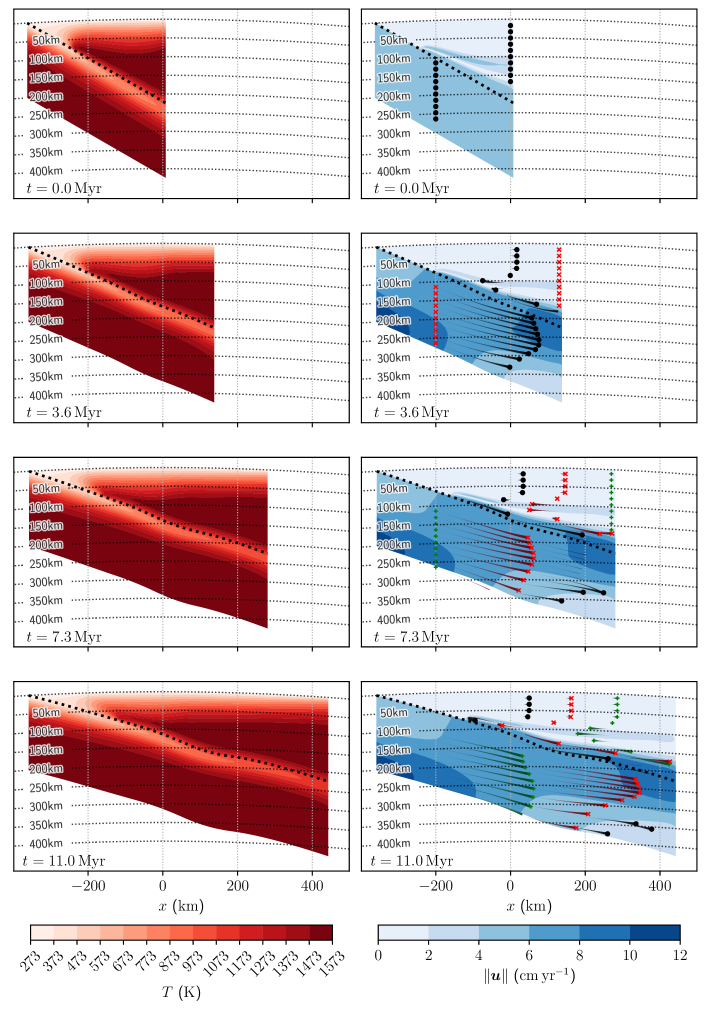
Figure 6: Temperatures and speeds around the evolving slab over $11\text{\,}\mathrm{Myr}$. The model is solved with $\mathcal{d}=2$ where the geometry is taken from a cross-section of the $\mathcal{d}=3$ volume parallel to the $y$-axis at location $y=$-200\text{\,}\mathrm{km}$$. The time interval is discretized with $100$ time steps such that $\Delta t=$0.11\text{\,}\mathrm{Myr}$$. Tracers are added in the speed plots showing pathlines between the time snapshots.

The temperature and velocity fields computed on the $\mathcal{d}=2$ cross-sections of the $\mathcal{d}=3$ geometry are shown in figures 6, LABEL:, 7, LABEL: and 8, respectively. Each row corresponds to time snapshots taken over the $t_{\text{slab}}=$11\text{\,}\mathrm{Myr}$$ model maximum time which has been discretized with $100$ time steps such that $\Delta t=$0.11\text{\,}\mathrm{Myr}$$. The slab B-spline is overlaid in each plot as a dotted line. Tracers are added in the velocity plots showing pathlines between the shown time snapshots. Should a tracer leave the geometry between each snapshot, it is removed from the visualization leaving only its remaining tail. The geometry deformation is not shown between snapshots and the tracers do not cross over $\Gamma_{\text{slab}}$ at any time in the simulation (though their pathlines may appear to do so).

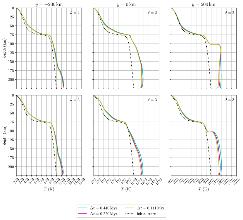
Figure 9: Temporal convergence test of the $\mathcal{d}=2$ models shown in figures 6, 7 and 8 and $\mathcal{d}=3$ models shown in figures 12, 13 and 14. Here, in each case, we plot the surface temperatures as a function of depth along $\Gamma_{\text{slab}}$ at final time $t(\vartheta=1)=$11\text{\,}\mathrm{Myr}$$. We also overlay the initial temperature along the slab at $t=0$ as a dotted line. For each case the temporal domain is discretized by $25$, $50$ and $100$ time steps yielding the time step sizes shown in the legend.

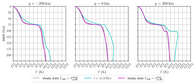
Figure 10: Comparison of the $\mathcal{d}=2$ model slab surface temperatures as a function of depth in the steady state on the initial geometry, time dependent $t=$11\text{\,}\mathrm{Myr}$$ and steady state on the final geometry.

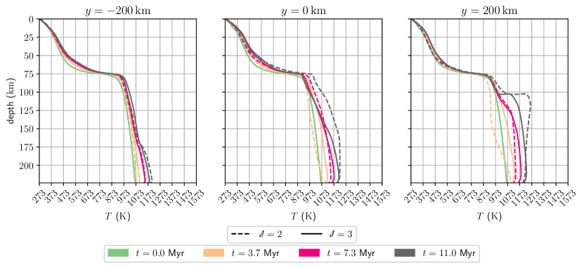
Figure 15: Comparison of the slab surface temperatures as a function of depth as modeled in the $\mathcal{d}=2$ and $\mathcal{d}=3$ cases. In each case, we plot the surface temperatures as a function of depth along $\Gamma_{\text{slab}}$ at the time steps shown in the $\mathcal{d}=2$ models in figures 6, 7 and 8 and the cross-sections of the $\mathcal{d}=3$ model in figures 12, 13 and 14. The difference between the $\mathcal{d}=2$ and $\mathcal{d}=3$ models at time $t=$0.0\text{\,}\mathrm{Myr}$$ is indistinguishable at this scale.

Convergence of the surface temperature as a function of time step size in the temporal discretization is shown in figure 9. In figure 10 we show the slab surface temperature as a function of depth as computed in the steady state on the initial geometry $S^{\mathrm{initial}}_{(\boldsymbol{\mathcal{p}},\boldsymbol{\Xi})}$, as computed in the full time dependent $\mathcal{d}=2$ model at time $t=t_{\text{slab}}$ and as the steady state on the final geometry $S^{\mathrm{final}}_{(\boldsymbol{\mathcal{p}},\boldsymbol{\Xi})}$. Finally, the temperature as a function of depth along $\Gamma_{\text{slab}}$ at the final time $t=t_{\text{slab}}$ are shown in figure 15.

5.2 3D slab

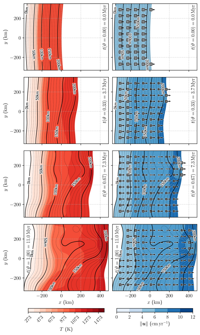
Figure 11: Computed $\mathcal{d}=3$ model slab surface temperatures and velocities with an initial $30\text{\,}\mathrm{\SIUnitSymbolDegree}$ straight dip evolving into the Nazca slab geometry over $11\text{\,}\mathrm{Myr}$ (cf. figure 1). The time interval is discretized with $100$ time steps such that $\Delta t=$0.11\text{\,}\mathrm{Myr}$$. In the instantaneous velocity plot, crosses represent velocity in the $-\hat{\boldsymbol{z}}$ direction (into the page) and arrows correspond to the velocity component acting in the $\hat{\boldsymbol{x}}$ and $\hat{\boldsymbol{y}}$ directions.

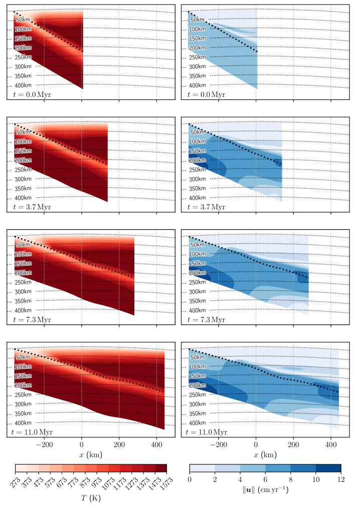
Figure 12: Cross-sectional temperature and speeds of the computed $\mathcal{d}=3$ model. The data presented is measured at the cross-section of the full volume parallel to the $y$-axis at location $y=$-200\text{\,}\mathrm{km}$$ (compare to $\mathcal{d}=2$ model in figure 6). The time domain is discretized with $100$ time steps such that $\Delta t=$0.11\text{\,}\mathrm{Myr}$$.

Snapshots of the $\mathcal{d}=3$ case temperature and velocity approximations evaluated on the slab interface are shown in figure 11. As in the $\mathcal{d}=2$ case we discretize the temporal domain with $100$ time steps such that $\Delta t=$0.11\text{\,}\mathrm{Myr}$$. Overlaid on the velocity plot are arrows indicating the direction of flow on the surface in the $\hat{\boldsymbol{x}}$ and $\hat{\boldsymbol{y}}$ directions along with cross markers with size corresponding to normalized speed in the $-\hat{\boldsymbol{z}}$ direction (into the page). Cross-sections of the temperature and velocity solution at $y=$-200\text{\,}\mathrm{km}$$, $0\text{\,}\mathrm{km}$, and $200\text{\,}\mathrm{km}$ are shown in figures 12, LABEL:, 13, LABEL: and 14, respectively. Tracers and their pathlines are not added to these velocity cross-sections due to the inability to visualize their $\hat{\boldsymbol{y}}$ component.

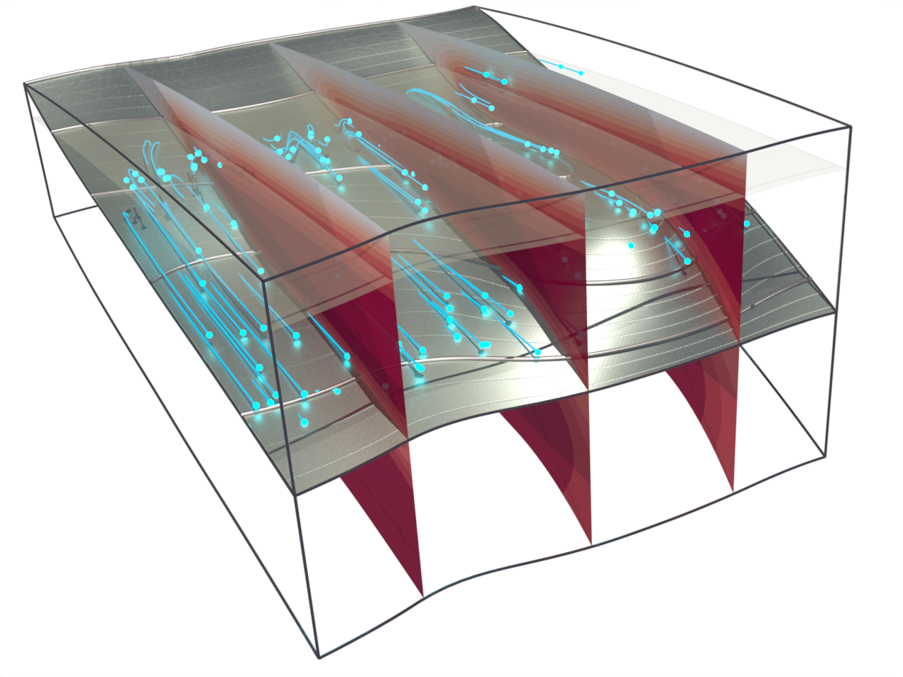
Figure 16: Rendering of the $\mathcal{d}=3$ model at time $t=t_{\text{slab}}$. Tracers are added where tails show $5.5\text{\,}\mathrm{Myr}$ long pathlines. Some pathlines cross through the slab interface shown; however, this is not an indication that the tracers have passed through the interface as the time evolving slab is not shown. There is very minor movement in the tracers located in the $\Omega_{\text{plate}}$, their displacement is dictated by the slab deformation above the plate depth $d_{\text{plate}}$ highlighted as a translucent layer. Pathlines close to the slab surface are dominated by the convergence component of the velocity boundary condition direction $\hat{\boldsymbol{d}}_{\text{conv}}=\hat{\boldsymbol{x}}$.

Cross-sections of the temperature field taken at constant $y=$-200\text{\,}\mathrm{km}$$, $0\text{\,}\mathrm{km}$, and $200\text{\,}\mathrm{km}$ as a function of depth along $\Gamma_{\text{slab}}$ at final time $t=t_{\text{slab}}$ is shown in figure 15. These data overlay the slab surface temperatures as a function of depth computed from the corresponding $\mathcal{d}=2$ models. Furthermore, convergence of the surface temperatures as a function of time step size in the temporal discretization at these cross sections is shown in figure 9. The volume of the $\mathcal{d}=3$ model at $t=t_{\text{slab}}$ with these cross-sections and additional path tracers is shown in figure 16.

5.3 Discussion

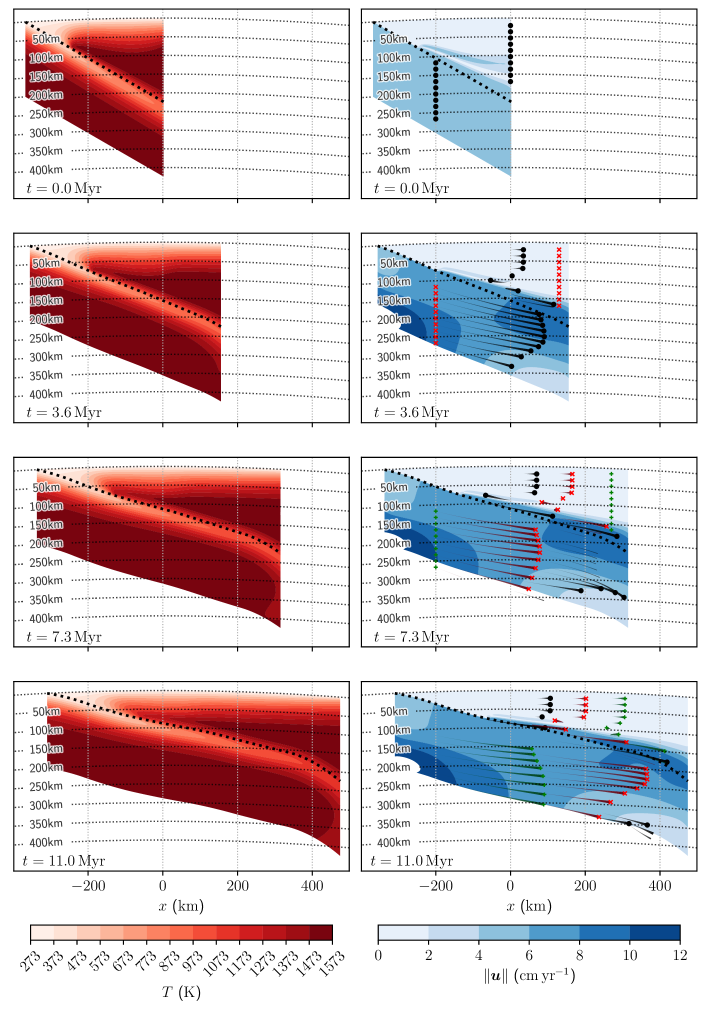
Figure 7: As Figure 6 but now for $y=$0\text{\,}\mathrm{km}$$.

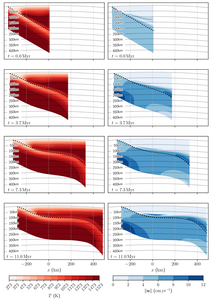
Figure 14: As figure 12 but now at $y=$200\text{\,}\mathrm{km}$$ (compare to $\mathcal{d}=2$ model in figure 8).

The surface temperatures computed from the $\mathcal{d}=2$ and $\mathcal{d}=3$ models shown in figure 15 indicate a warming of the slab above the coupling point. This appears to be caused by the slab surface transitioning to a shallower angle than the initial condition, pushing the surface into a warmer region of the wedge (see figures 6, 7, 8, 12, 13 and 14). Examining the $y=$200\text{\,}\mathrm{km}$$ cross-section in figure 14 the slab surface does not evolve to a much shallower depth as in the $y=$-200\text{\,}\mathrm{km}$$ and $y=$0\text{\,}\mathrm{km}$$ cross-section cases. This corresponds with the less significant warming of the slab surface above $d_{c}$. Consider also the slab surface temperatures shown in figure 10 which increase as the slab evolves from the initial steady state to $t=t_{\text{slab}}$, and cools when evolved to the steady state with no further slab deformation.

In all cases the steady state solution used for the initial temperature field $T_{h}^{n=0}$ exhibits a diffusive thickening of the plate within the approximate depths of $50\text{\,}\mathrm{km}$ and $100\text{\,}\mathrm{km}$. This feature persists through the simulation and is displaced by the slab deformation. Future models may be improved by prescribing the initial temperature field computed from an unsteady simulation run to a time just after transient effects become negligible.

The configuration of the slab surface temperature in the $\mathcal{d}=3$ case shown in figure 11 is largely dictated by the velocity boundary condition applied to $\Gamma_{\text{slab}}$. Choosing $\hat{\boldsymbol{d}}_{\text{conv}}=\hat{\boldsymbol{x}}$ restricts the velocity profile to be very similar to the $\mathcal{d}=2$ cases along $\Gamma_{\text{slab}}$. Deviating from this decision, one avenue is to choose $\hat{\boldsymbol{d}}_{\text{conv}}=-\hat{\boldsymbol{z}}$ which would yield a convergence velocity in the direction of steepest descent. However in this case, the flow above and below $\Gamma_{\text{slab}}$ will become unreasonable for the subduction zone model as a result of satisfying mass conversation, $\nabla\cdot\boldsymbol{u}=0$. These flows, which are not realistic in a subduction zone model, typically form as velocity fields impinging or jetting out from $\Gamma_{\text{slab}}$ in order to account for diverging and converging flows on the $\Gamma_{\text{slab}}$ topology, respectively. An approach to alleviate this issue is to solve for some component of the flow, $\boldsymbol{u}$, on $\Gamma_{\text{slab}}$ implicitly. For example, the velocity prescription on $\Gamma_{\text{slab}}$ could be changed such that only the $\hat{\boldsymbol{\tau}}_{\text{conv}}$ component is imposed allowing the remaining tangential component in the $\hat{\boldsymbol{\tau}}^{\bot}_{\text{conv}}$ direction to be implicit in the model. This however introduces an issue where the deformation velocity component, $(\boldsymbol{u}_{\text{slab}}\cdot\hat{\boldsymbol{\tau}}^{\bot}_{\text{conv}})\hat{\boldsymbol{\tau}}^{\bot}_{\text{conv}}$, must be neglected. Another approach would be to impose a convergence velocity $\boldsymbol{u}_{\text{conv}}$, such that $\boldsymbol{u}|_{\Gamma_{\text{slab}}}=\boldsymbol{u}_{\text{conv}}+\boldsymbol{u}_{\text{slab}}$, which is computed from a Stokes problem of topological dimension $\mathcal{d}-1$ defined on $\Gamma_{\text{slab}}$. The divergence free constraint defined on the topology of the surface would then ensure no regions of converging or diverging flow. However, the complexity of the mathematical formulation of this problem as well as its implementation for parallel computation is challenging.

The slab temperature approximation close to $\partial\Omega_{\text{slab outlet}}$ and $\partial\Omega_{\text{wedge outlet}}$ is significantly affected by the non-overlapping component of the interpolation operation $\mathcal{P}(\cdot)$ described in section 3.5. This is indicated, for example, in the $t>0$ cases of figure 15 at depths below $215\text{\,}\mathrm{km}$ (i.e. the component of the $\Gamma_{\text{slab}}$ closest to $\partial\Omega_{\text{slab outlet}}$ and $\partial\Omega_{\text{wedge outlet}}$). One can see a small downturn in the temperature which arises from interpolation of $T_{\text{out}}$ (equation 11) which is colder than the material in the volume which is displaced by the moving slab. This issue could be addressed by ensuring all meshes overlap such that the overall volume remains consistent negating the need for non-overlapping interpolation. However, this would introduce a large computational cost resolving a volume which is largely spatially removed from the domain of interest close to $\Gamma_{\text{slab}}$.

The decision to choose the B-spline properties $\boldsymbol{p}_{i}=2$ and $n_{i}+1=8$, $i=1,\ldots,\mathcal{d}-1$, was made to balance production of a robust numerical model against the performance of iterative solvers applied to the linear system underlying the Stokes problem. Choosing a greater fidelity in the knot vector lead to degradation of the rate of convergence of the FGMRES method for seismic data which exhibit rapid non-smooth changes in the slab geometry. Future development of the model would investigate methods to retain the robust solution of the velocity and pressure approximations with greater spatial fidelity of $\Gamma_{\text{slab}}$. Additionally the geometric operations required to define the volume using CAD as described in section 3.3 become prohibitively expensive as the B-spline approximation order and control point vectors’ cardinality increases.

We finish discussion on the caution that these models are in sensu stricto based on a toy model (if admittedly a complicated one). The results presented here should be interpreted to indicate that precise description of the slab evolving geometry leads to significant differences between 3D models and 2D cross-sections, but the temperature-pressure paths should not be used to compare directly to existing slab models or observations of flat slab subduction. In future work we will apply this modeling frame work to regions of flat slab subduction with locally adjusted parameters for geometry, coupling point, structure of the overriding plate, etc.

6 Conclusion

We have devised, implemented, and demonstrated a numerical model of a subduction zone which accounts for a kinematic prescription of a geometry evolving slab surface. We do this by approximating seismic observation of slab geometries with a B-spline. By constructing a deformation path for the B-spline surface from an initial to a final slab geometry, we are able to evolve this prescribed slab surface geometry over time. Enveloping the slab surface spline in a volume using CAD allows us to create a sequence of meshes in which we compute approximations of velocity, pressure and temperature of a subduction zone model discretized by the FE method.

Appendix A Model equations rescaling

Using velocity, length and viscosity scales $u_{r}$, $h_{r}$ and $\eta_{r}$, respectively we define the rescaled quantities

$$\boldsymbol{u} =u_{r}\boldsymbol{u}^{\prime},\quad\boldsymbol{x}=h_{r}\boldsymbol{x}^{\prime},\quad\eta=\eta_{r}\eta^{\prime},$$

$$\nabla =\frac{1}{h_{r}}\nabla^{\prime},\quad t=\frac{h_{r}}{u_{r}}t^{\prime},\quad k=h_{r}u_{r}k^{\prime},\quad Q=\frac{u_{r}}{h_{r}}Q^{\prime}.$$ (33)

Employing these quantities we arrive at the rescaled Stokes-energy formulation of equations 1, 2 and 3 where we seek $\boldsymbol{u}^{\prime}$, $p^{\prime}$ and $T^{\prime}$ such that

$$-\eta_{r}\frac{u_{r}}{h_{r}^{2}}\nabla^{\prime}\cdot\sigma^{\prime} =\boldsymbol{0},$$ (34)

$$\frac{u_{r}}{h_{r}}\nabla^{\prime}\cdot\boldsymbol{u}^{\prime} =0,$$ (35)

$$\rho c_{p}\left(\frac{u_{r}}{h_{r}}\mathinner{\dfrac{\partial{}T}{\partial{{t^{\prime}}}}}+\frac{u_{r}}{h_{r}}\boldsymbol{u}^{\prime}\cdot\nabla^{\prime}T\right)-\frac{h_{r}u_{r}}{h_{r}^{2}}\nabla^{\prime}\cdot\left(k^{\prime}\nabla^{\prime}T\right) =\frac{u_{r}}{h_{r}}Q^{\prime},$$ (36)

which after simplification reads

$$-\nabla^{\prime}\cdot\sigma^{\prime} =\boldsymbol{0},$$ (37)

$$\nabla^{\prime}\cdot\boldsymbol{u}^{\prime} =0,$$ (38)

$$\rho c_{p}\left(\mathinner{\dfrac{\partial{}T}{\partial{{t^{\prime}}}}}+\boldsymbol{u}^{\prime}\cdot\nabla^{\prime}T\right)-\nabla^{\prime}\cdot\left(k^{\prime}\nabla^{\prime}T\right) =Q^{\prime}.$$ (39)

The numerical values used in our computations are $h_{r}=$1\text{\,}\mathrm{km}$$, $u_{r}=$5\text{\,}\mathrm{cm}\text{\,}{\mathrm{yr}}^{-1}$$ and $\eta_{r}=${10}^{21}\text{\,}\mathrm{Pa}$$.

Abbreviations

B-spline: Bézier spline; CAD: Computer-Aided Design; DoF: Degree of Freedom; FE: Finite element; FFC: FEniCS Form Compiler; FGMRES: Flexible Generalized Minimal Residual; GMRES: Generalized Minimal Residual; iLU: incomplete LU; PDE: Partial Differential Equation; PETSc: Portable Extensible Toolkit for Scientific computation; UFL: Unified Form Language.

Availability of data and material

An implementation of the subduction zone model is provided at https://github.com/nate-sime/mantle-convection.

The data generated by the subduction zone model code and presented in this paper is available in Sime et al. (2023).

Competing interests

The authors declare that they have no competing interest.

Funding

This work was supported by National Science Foundation grant 2021027.

Authors’ contributions

NS developed and tested the FEniCS finite element approach in collaboration with CW. PvK aided in benchmarking the 2D subduction zone models. All contributed to writing the manuscript.

Endnotes

Figure 1: Subduction zone interface geometry data points as retrieved from seismological observations. The resolution of the data is highlighted along the border of Chile and Argentina. Geometry of the present-day structure of the flat slab segment is based on Anderson et al. (2007).

Figure 8: As Figure 6 but now for $y=$200\text{\,}\mathrm{km}$$.

Figure 13: As figure 12 but now at $y=$0\text{\,}\mathrm{km}$$ (compare to $\mathcal{d}=2$ model in figure 7).

References

- Abers et al. (2013) Abers, G.A, Nakajima, J, van Keken, P.E, Kita, S, Hacker, B.R (2013) Thermal-petrological controls on the location of earthquakes within subducting plates. Earth Planet Sci Lett 369–370, 178–187. doi:10.1016/j.epsl.2013.03.022
- Abers et al. (2020) Abers, G.A, van Keken, P.E, Wilson, C.R (2020) Deep decoupling in subduction zones: Observations and temperature limits. Geosphere 16, 1408–1424. doi:10.1130/GES02278.1
- Alnæs et al. (2014) Alnæs, M.S, Logg, A, Ølgaard, K.B, Rognes, M.E, Wells, G.N (2014) Unified Form Language: A domain-specific language for weak formulations of partial differential equations. ACM Trans Math Softw 40, 1–37. doi:10.1145/2566630
- Anderson et al. (2007) Anderson, M, Alvarado, P, Zandt, G, Beck, S (2007) Geometry and brittle deformation of the subducting Nazca Plate, Central Chile, and Argentina. Geophys J Inter 171, 419–434. doi:10.1111/j.1365-246X.2007.03483.x
- Antonijevic et al. (2015) Antonijevic, S.K, Wagner, L.S, Beck, S.L, Long, M.D, Zandt, G, Tavera, H (2015) The role of ridges in the formation and longevity of flat slabs. Nature 524, 212–215. doi:10.1038/nature14648
- Axen et al. (2018) Axen, G.J, van Wijk, J.W, Currie, C.A (2018) Basal continental mantle lithosphere displaced by flat-slab subduction. Nat Geosci 11, 961–964. doi:10.1038/s41561-018-0263-9
- Balay et al. (2019) Balay, S, Abhyankar, S, Adams, M.F, Brown, J, Brune, P, Buschelman, K, Dalcin, L, Dener, A, Eijkhout, V, Gropp, W.D, Karpeyev, D, Kaushik, D, Knepley, M.G, May, D.A, McInnes, L.C, Mills, R.T, Munson, T, Rupp, K, Sanan, P, Smith, B.F, Zampini, S, Zhang, H, Zhang, H (2019) PETSc Users Manual. https://www.mcs.anl.gov/petsc
- Balay et al. (2023) Balay, S, Abhyankar, S, Adams, M.F, Benson, S, Brown, J, Brune, P, Buschelman, K, Constantinescu, E.M, Dalcin, L, Dener, A, Eijkhout, V, Faibussowitsch, J, Gropp, W.D, Hapla, V, Isaac, T, Jolivet, P, Karpeev, D, Kaushik, D, Knepley, M.G, Kong, F, Kruger, S, May, D.A, McInnes, L.C, Mills, R.T, Mitchell, L, Munson, T, Roman, J.E, Rupp, K, Sanan, P, Sarich, J, Smith, B.F, Zampini, S, Zhang, H, Zhang, H, Zhang, J (2023) PETSc Web page. https://www.mcs.anl.gov/petsc
- Bebout and Penniston-Dorland (2016) Bebout, G.E, Penniston-Dorland, S.C (2016) Fluid and mass transfer at subduction interfaces – The field metamorphic record. Lithos 240–243, 228–258. doi:10.1016/j.lithos.2015.10.007
- Bengtson and van Keken (2012) Bengtson, A.K, van Keken, P.E (2012) Three-dimensional thermal structure of subduction zones: effects of obliquity and curvature. Solid Earth 3, 365–373. doi:10.5194/se-3-365-2012
- Bingol and Krishnamurthy (2019) Bingol, O.R, Krishnamurthy, A (2019) NURBS-Python: An open-source object-oriented NURBS modeling framework in Python. SoftwareX 9, 85–94. doi:10.1016/j.softx.2018.12.005
- Bloch et al. (2018) Bloch, W, John, T, Kummerow, J, Salazar, P, Krüger, O, Shapiro, S (2018) Watching dehydration: Seismic indication for transient fluid pathways in the oceanic mantle of the subducting Nazca slab. Geochem Geophys Geosys 19, 3189–3207. doi:10.1029/2018GC007703
- Carrapa et al. (2019) Carrapa, B, DeCelles, P.G, Romero, M (2019) Eartly inception of the Laramide Orogeny in Southwestern Monta and Northern Wyoming: Implications for models of flat-slab subduction. J Geophys Res: Solid Earth 124, 2102–2123. doi:10.1029/2018JB016888
- Cerpa et al. (2017) Cerpa, N.G, Wada, I, Wilson, C.R (2017) Fluid migration in the mantle wedge: Influence of mineral grain size and mantle compaction. J Geoph Res: Solid Earth 122, 6247–6268. doi:10.1002/2017JB014046
- Contreras-Reyes et al. (2019) Contreras-Reyes, E, Muñoz-Linford, P, Cortes-Rivas, V, Bello-Gonzales, J.P, Ruiz, J.A, Krabbenhöft, A (2019) Structure of the collision zone between the Nazca Ridge and the Peruvian convergent margin: Geodynamic and seismotectonic implications. Tectonics 38, 3416–3435. doi:10.1029/2019TC005637
- Currie and Copeland (2022) Currie, C.A, Copeland, P (2022) Numerical models of Farallon plate subduction: Creating and removing a flat slab. Geosphere 18, 476–502. doi:01.1130/GES02391.1
- Dokken (2022) Dokken, J.S DOLFINx-MPC v0.5.0. https://github.com/jorgensd/dolfinx_mpc
- English et al. (2003) English, J.M, Johnston, S.T, Wang, K (2003) Thermal modeling of the Laramide orogeny: testing the flat slab subduction hypothesis. Earth Planet Sci Lett 214, 619–632. doi:10.1016/S0012-821X(03)00399-6
- Fan and Carrapa (2014) Fan, M, Carrapa, B (2014) Late Cretaceous-early Eocene Laramide uplift, exhumation, and basin subsidence in Wyoming: Crustal responses to flat slab subduction. Tectonics 33, 509–529. doi:10.1002/2012TC003221
- Finzel et al. (2011) Finzel, E.S, Trop, J.M, Ridgway, K.D, Enkelmann, E (2011) Upper plate proxies for flat-slab subduction processes in southern Alaska. Earth Planet Sci Lett 303, 348–360. doi:10.1016/j.epsl.2011.01.014
- Gamblin et al. (2015) Gamblin, T, LeGendre, M.P, Collette, M.R, Lee, G.L, Moody, A, de Supinski, B.R, Futral, W.S (2015) The Spack Package Manager: Bringing order to HPC software chaos. In: Supercomputing 2015 (SC’15), Austin, Texas. Art No 40, doi:10.1145/2807591.2807623
- Gerya et al. (2009) Gerya, T.V, Fossati, D, Cantieni, C, Seward, D (2009) Dynamic effects of aseismic ridge subduction: numerical modeling. Eur J Miner 21, 649–661. doi:10.1127/0935-1221/2009/0021-1931
- Geuzaine and Remacle (2009) Geuzaine, C, Remacle, J-F (2009) Gmsh: A 3-D finite element mesh generator with built-in pre- and post-processing facilities. Int J Numer Meth Engin 79, 1309–1331. doi:10.1002/nme.2579
- Gutscher and Peacock (2003) Gutscher, M-A, Peacock, S.M (2003) Thermal models of flat subduction and the rupture zone of great subduction earthquakes. J Geoph Res: Solid Earth 108. Art No 2009, doi:10.1029/2001JB000787
- Gutscher et al. (1999) Gutscher, M-A, Olivet, J-L, Aslanian, D, Eissen, J-P, Maury, R (1999) The ”lost Inca Plateau”: cause of flat subduction beneath Peru. Earth Planet Sci Lett 14, 395–410. doi:10.1130/GES01537.1
- Houston and Sime (2018) Houston, P, Sime, N (2018) Automatic symbolic computation for discontinuous Galerkin finite element methods. SIAM J Sci Comp 40, 327–357. doi:10.1137/17M1129751
- Jadamec and Haynie (2017) Jadamec, M.A, Haynie, K.L (2017) Tectonic drives of the Wrangell block: Insights on fore-arc sliver processes from 3-D geodynamic models of Alaska. Tectonics 36, 1180–1206. doi:10.1002/2016TC004410
- Jadamec et al. (2013) Jadamec, M.A, Billen, M.I, Roeske, S.M (2013) Three-dimensional numerical models of flat slab subduction and the Denali fault driving deformation in south-central Alaska. Earth Planet Sci Lett 376, 29–42. doi:10.1016/j.epsl.2013.06.009
- Jones et al. (2021) Jones, T.D, Sime, N, van Keken, P.E (2021) Burying Earth’s primitive mantle in the slab graveyard. Geochem Geophys Geosys 22. Art No e2020GC009396, doi=10.1029/2020GC009396
- Jung et al. (2004) Jung, H, Green II, H.W, Dobrzhinetskaya, L.F (2004) Intermediate-depth earthquake faulting by dehydration embrittlement with negative volume change. Nature 428, 545–549. doi:10.1038/nature02412
- Karato and Wu (1993) Karato, S, Wu, P (1993) Rheology of the upper mantle: A synthesis. Science 260, 771–778. doi:10.1126/science.260.5109.771
- Kelemen and Hirth (2007) Kelemen, P.B, Hirth, G (2007) A periodic shear-heating mechanism for intermediate-depth earthquakes in the mantle. Nature 446, 787–790. doi:10.1038/nature05717
- Kirby and Logg (2006) Kirby, R.C, Logg, A (2006) A compiler for variational forms. ACM Trans Math Softw 32, 417–444. doi:10.1145/1163641.1163644
- Kneller and van Keken (2012) Kneller, E.A, van Keken, P.E (2012) The effects of three-dimensional slab geometry on deformation in the mantle wedge: Implications for shear wave anisotropy. Geochem Geophys Geosys 9. Art No Q01006, doi:10.1029/2008GC002151
- Li and Li (2007) Li, Z-X, Li, X-H (2007) Formation of the 1300-km-wide intracontinental orogen and postorogenic magmatic province in Mesozoic South China. Geology 35, 179–182. doi:10.10130/G23193A.1
- Liu et al. (2008) Liu, L, Spasojevič, S, Gurnis, M (2008) Reconstructing Farallon plate subduction beneath North America back to the late Cretaceous. Science 322, 934–938. doi:11.126/science.1162921
- Liu et al. (2022) Liu, X, Currie, C.A, Wagner, L.S (2022) Cooling of the continental plate during flat-slab subduction. Geosphere 18, 49–68. doi:10.1130/GES02402.1
- Logg and Wells (2010) Logg, A, Wells, G.N (2010) DOLFIN: Automated finite element computing. ACM Trans Math Softw 37, 1–28. doi:10.1145/1731022.1731030
- Logg et al. (2012) Logg, A, Mardal, K-A, Wells, G.N (eds.) (2012) Automated Solution of Differential Equations by the Finite Element Method. Lecture Notes in Computational Science and Engineering, vol 84. Springer, Heidelberg, Germany
- Manea and Manea (2011) Manea, V.C, Manea, M (2011) Flat-slab thermal structure and evolution beneath Central Mexico. Pure Appl Geophys 168, 1475–1487. doi:10.1007/s00024-010-0207-9
- Manea et al. (2017) Manea, V.C, Manea, M, Ferrari, L, Orozco-Esquivel, T, Valenzuela, R.W, Husker, A, Kostoglodov, V (2017) A review of the geodynamic evolution of flat slab evolution in Mexico, Peru, and Chile. Tectonophysics 695, 27–52. doi:10.1016/j.tecto.2016.11.037
- Marot et al. (2014) Marot, M, Monfret, T, Gerbault, M, Nolet, G, Ranalli, G, Pardo, M (2014) Flat versus normal subduction zones: a comparison based on 3-D regional traveltime tomography and petrological modelling of central Chile and western Argentia (29∘C–35∘S). Geophys J Int 199, 1633–1654. doi:10.1093/gji/ggu355
- May and Moresi (2008) May, D.A, Moresi, L (2008) Preconditioned iterative methods for Stokes flow problems arising in computational geodynamics. Phys Earth Planet Inter 171, 33–47
- Molnar and England (1990) Molnar, P, England, P (1990) Temperature, heat flux, and frictional stress near major thrust faults. J Geoph Res: Solid Earth 95, 4833–4856. doi:10.1029/JB095iB04p04833
- Nitsche (1971) Nitsche, J (1971) Über ein Variationsprinzip zur Lösung von Dirichlet-Problemen bei Verwendung von Teilräumen, die keinen Randbedingungen unterworfen sind. In: Abhandlungen aus dem Mathematischen Seminar der Universität Hamburg, vol 36, pp 9–15
- Open CASCADE Technology (2022) Open CASCADE Technology Open CASCADE Technology. www.opencascade.com
- Peacock and Wang (1999) Peacock, S.M, Wang, K (1999) Seismic consequences of warm versus cool subduction metamorphisms: Examples from southwest and northeast Japan. Science 286, 937–939. doi:10.1126/science.286.5441.937
- Piegl and Tiller (1997) Piegl, L, Tiller, W (1997) The NURBS Book, Second Edition. Monographs in Visual Communication. Springer, Heidelberg, Germany
- Plunder et al. (2018) Plunder, A, Thieulot, C, van Hinsbergen, D.J.J (2018) The effect of obliquity on temperature in subduction zones: insights from 3-D numerical modeling. Solid Earth 9, 759–776. doi:10.5194/se-9-759-2018
- Raleigh and Paterson (1965) Raleigh, C.B, Paterson, M.S (1965) Experimental deformation of serpentinite and its tectonic implications. J Geophys Res: Solid Earth 70, 3965–3985. doi:10.1029/JZ070i016p03965
- Richardson et al. (2019) Richardson, C.N, Sime, N, Wells, G.N (2019) Scalable computation of thermomechanical turbomachinery problems. Fin Elem Analys Design 155, 32–42. doi:10.1016/j.finel.2018.11.002
- Rosas et al. (2016) Rosas, J.C, Currie, C.A, He, J (2016) Three-dimensional thermal model of the Costa Rica-Nicaragua subduction zone. Pure Appl Geophys 173, 3317–3339. doi:10.1007/s00024-015-1197-4
- Saad (1993) Saad, Y (1993) A flexible inner-outer preconditioned GMRES algorithm. SIAM J Sci Comp 14, 461–469. doi:10.1137/0914028
- Saad and Schultz (1986) Saad, Y, Schultz, M.H (1986) GMRES: A generalized minimal residual algorithm for solving nonsymmetric linear systems. SIAM J Sci Stat Comp 7, 856–869. doi:10.1137/0907058
- Schmid et al. (2002) Schmid, C, Goes, S, van der Lee, S, Giardini, D (2002) Fate of the Cenozoic Farralon slab from a comparison of kinematic thermal modeling with tomographic images. Earth Planet Sci Lett 204, 17–32. doi:10.1016/S0012-821X(02)00985-8
- Scroggs et al. (2022) Scroggs, M.W, Dokken, J.S, Richardson, C.N, Wells, G.N (2022) Construction of arbitrary order finite element degree-of-freedom maps on polygonal and polyhedral cell meshes. ACM Trans Math Softw 48. Art No 18, doi:10.1145/3524456
- Shiina et al. (2013) Shiina, T, Nakajima, J, Matsuzawa, T (2013) Seismic evidence for high pore pressures in oceanic crust: Implications for fluid-related embrittlement. Geoph Res Lett 40, 2006–2010. doi:10.1002/grl.50468
- Shiina et al. (2017) Shiina, T, Nakjima, J, Matsuzawa, T, Toyokuni, G, Kita, S (2017) Depth variations in seismic velocity in the subducting crust: Implications for fluid-related embrittled for intermediate-depth earthquakes. Geophys Res Lett 44, 810–817. doi:10.1002/2016GL071798
- Shirey et al. (2021) Shirey, S.B, Wagner, L.S, Walter, M.J, Pearson, D.G, van Keken, P.E (2021) Slab transport of fluids to deep focus earthquake depths – thermal modeling constraints and evidence from diamonds. AGU Advances 2. Art No e2020AV000304, doi:10.1029/2020AV000304
- Sime et al. (2021) Sime, N, Maljaars, J.M, Wilson, C.R, van Keken, P.E (2021) An exactly mass conserving and pointwise divergence free velocity method: Application to compositional buoyancy driven flow problems in geodynamics. Geochem Geophys Geosys 22. Art No e2020GC009349, doi:10.1029/2020GC009349
- Sime et al. (2022) Sime, N, Wilson, C.R, van Keken, P.E (2022) A pointwise conservative method for thermochemical convection under the compressible anelastic liquid approximation. Geochem Geophys Geosys 23. Art No e2021GC009922, doi:10.1029/2021GC009922
- Sime et al. (2023) Sime, N, Wilson, C.R, van Keken, P.E (2023) Thermal modeling of subduction zones with prescribed and evolving 2D and 3D slab geometries data (1.0) [Data set]. Zenodo. doi:10.5281/zenodo.8350532
- Sippl et al. (2019) Sippl, C, Schurr, B, John, T, Hainzl, S (2019) Filling the gap in a double seismic zone: Intraslab seismicity in northern Chile. Lithos 346–347. Art No 105155, doi:10.1016/j.lithos.2019.105155
- Syracuse et al. (2010) Syracuse, E.M, van Keken, P.E, Abers, G.A (2010) The global range of subduction zone thermal models. Phys Earth Planet Inter 183, 73–90. doi:10.1016/j.pepi.2010.02.004
- Taramón et al. (2015) Taramón, J.M, Rodríguez-González, J, Negredo, A.M, Billen, M.I (2015) Influence of cratonic lithosphere on the formation and evolution of flat slabs: Insights from 3-D time-dependent modeling. Geochem Geophys Geosys 16, 2933–2948. doi:doi.1002/2015GC005940
- Taylor and Hood (1973) Taylor, C, Hood, P (1973) A numerical solution of the Navier–Stokes equations using the finite element technique. Comput Fluids 1, 73–100
- van den Berg et al. (2015) van den Berg, A.P, Segal, G, Yuen, D.A (2015) SEPRAN: A versatile finite-element package for a wide variety of problems in geosciences. J Earth Sci 26, 89–95. doi:10.1007/s12583-015-0508-0
- van Keken and Wilson (2023) van Keken, P.E, Wilson, C.R (2023) An introductory review of the thermal structure of subduction zones: I – motivation and selected examples. Prog Earth Planet Sci 10. Art No 42, doi:10.1186/s40645-023-00573-z
- van Keken et al. (2002) van Keken, P.E, Kiefer, B, Peacock, S.M (2002) High-resolution models of subduction zones: Implications for mineral dehydration reactions and the transport of water to the deep mantle. Geochem Geophys Geosys 3. Art No 1056, doi=10.1029/2001GC000256
- van Keken et al. (2012) van Keken, P.E, Kita, S, Nakajima, J (2012) Thermal structure and intermediate-depth seismicity in the Tohoku-Hokkaido subduction zones. Solid Earth 3, 355–364. doi:10.5194/se-3-355-2012
- van Keken et al. (2019) van Keken, P.E, Wada, I, Sime, N, Abers, G.A (2019) Thermal structure of the forearc in subduction zones: A comparison of methodologies. Geochem Geophys Geosys 20, 3268–3288. doi:10.1029/2019GC008334
- van Keken et al. (2008) van Keken, P.E, Currie, C, King, S.D, Behn, M.D, Cagnioncle, A, He, J, Katz, R.F, Lin, S-C, Parmentier, E.M, Spiegelman, M, Wang, K (2008) A community benchmark for subduction zone modeling. Phys Earth Planet Inter 171, 187–197. doi:10.1016/j.pepi.2008.04.015
- Wada and He (2017) Wada, I, He, J (2017) Thermal structure of the Kanto region, Japan. Geoph Res Lett 44, 7194–7202. doi:10.1002/2017GL073597
- Wada and Wang (2009) Wada, I, Wang, K (2009) Common depth of slab-mantle decoupling: Reconciling diversity and uniformity of subduction zones. Geochem Geophys Geosys 10. Art No Q10009, doi:10.1029/2009GC002570
- Wagner et al. (2017) Wagner, L.S, Jaramillo, S, Ramirez-Hoyos, L.F, Monsalve, A, Cardona, A, Becker, T.W (2017) Transient slab flattening beneath Colombia. Geophys Res Lett 44, 6616–6623. doi:10.1002/2017GL073981
- Wagner et al. (2020) Wagner, L.S, Caddick, M.J, Kumar, A, Beck, S.L, Long, M.D (2020) Effects of oceanic crustal thickness on intermediate depth seismicity. Front Earth Sci 8. Art No 244, doi:10.3389/feart.2020.00244
- Wei et al. (2017) Wei, S.S, Wiens, D.A, van Keken, P.E, Cai, C (2017) Slab temperature control on the Tonga double seismic zone and slab mantle dehydration. Sci Adv 3. Art No e1601755, doi:10.1126/sciadv.1601755
- Wilson et al. (2017) Wilson, C.R, Spiegelman, M, van Keken, P.E (2017) TerraFERMA: The Transparent Finite Element Rapid Model Assembler for multiphysics problems in Earth sciences. Geochem Geophys Geosys 18, 769–810. doi:10.1002/2016GC006702
- Wilson et al. (2014) Wilson, C.R, Spiegelman, M, van Keken, P.E, Hacker, B.R (2014) Fluid flow in subduction zones: The role of solid rheology and compaction pressure. Earth Planet Sci Lett 401, 261–274. doi:10.1016/j.epsl.2014.05.052