Bayesian optimisation approach to quantify the effect of input parameter uncertainty on predictions of numerical physics simulations

Abstract

An understanding of how input parameter uncertainty in the numerical simulation of physical models leads to simulation output uncertainty is a challenging task. Common methods for quantifying output uncertainty, such as performing a grid or random search over the model input space, are computationally intractable for a large number of input parameters, represented by a high-dimensional input space. It is therefore generally unclear as to whether a numerical simulation can reproduce a particular outcome (e.g. a set of experimental results) with a plausible set of model input parameters. Here, we present a method for efficiently searching the input space using Bayesian Optimisation to minimise the difference between the simulation output and a set of experimental results. Our method allows explicit evaluation of the probability that the simulation can reproduce the measured experimental results in the region of input space defined by the uncertainty in each input parameter. We apply this method to the simulation of charge-carrier dynamics in the perovskite semiconductor methyl-ammonium lead iodide MAPbI₃ that has attracted attention as a light harvesting material in solar cells. From our analysis we conclude that the formation of large polarons, quasiparticles created by the coupling of excess electrons or holes with ionic vibrations, cannot explain the experimentally observed temperature dependence of electron mobility.

The following article has been submitted to APL Machine Learning. After it is published, it will be found at https://publishing.aip.org/resources/librarians/products/journals/

1 Introduction

Numerical simulation of physical models typically require a large number of input parameters that must be derived from previous theoretical calculations or measured experimentally [5, 7]. It is therefore inevitable that model input parameters suffer from uncertainty, and the effect of this uncertainty on the simulation output is not often discussed. Quantifying the functional relationship between the model input parameters and simulation output, in the $N$-dimensional input space where a set of $N$ model input parameters is a point in this space, is computationally challenging due to the combination of a high-dimensional input space and expensive numerical simulation times [32]. The effect of input uncertainty is thus routinely ignored given that naive methods for exploring the input space, such as grid or random search, require a computationally intractable number of simulations. It is therefore difficult to establish whether it is possible to generate a particular outcome, e.g. matching a set of experimental results, from a numerical simulation with a plausible set of input parameter values.

Machine learning, specifically Bayesian Optimisation [13, 41], can be used to efficiently search the input space in the region defined by the uncertainty in each input parameter, while minimising the difference between the simulation output and the experimentally measured result. During optimisation a probabilistic function is learned that maps the input parameters to the simulation output. This function explicitly evaluates the probability that the simulation can reproduce the experimental result in the region of input parameter space defined by the uncertainty. With this approach, informed conclusions can be drawn from the simulation output that allow for the uncertainty present in the input parameters. The method presented here falls into the wider field of statistical emulation for sensitivity and uncertainty analysis [8, 9, 10].

In the field of semiconductor physics, previous methods have attempted to manually minimise the error between simulation and experiment in the context of device parameter estimation for organic light-emitting diodes (OLEDs) [35, 27, 37]. However, a machine-learning method for automatically quantifying the effect of input parameter uncertainty on simulation prediction by minimising the error between simulation and experiment has not been established. A related problem, of utilising simulation prediction to find device parameters from experimental measurements, was demonstrated by Knapp et al. [39].

We demonstrate the method with application to the simulation of charge-carrier dynamics in lead-halide perovskites, LHPs. LHPs as light-harvesting layers in solar cells have been the focus of intense research activity due to power conversion efficiency increases of 9-27$\%$ since 2009 [33, 17] and low-energy low-cost manufacturing [21]. However, a comprehensive theoretical understanding of the mechanisms responsible for a number of their electronic properties is currently lacking [25, 26]. Specifically, the fundamental physical mechanisms controlling transport of photogenerated charge carriers is actively debated, see for example the measurements of Kobbekaduwa et al [42] on ultrafast dynamics that address the carrier mobility dependence on temperature in LHPs. Mesoscale simulation models of charge transport in LHPs, such as BoltMC - an ensemble Monte Carlo approach using Boltzmann transport theory [38], can provide insight into these mobility-limiting mechanisms.

Here we investigate the possibility that the formation of large polarons [22], quasi-particles resulting from the coupling of charge carriers with the surrounding polarised ionic lattice, affects the temperature dependence of the carrier mobility in methyl-ammonium lead iodide, MAPbI₃. A large polaron is an itinerant particle, with a mobility that decreases with temperature [38]. Prior theoretical work has utilised many approaches for calculating this dependence [22, 29, 4], parameterised from electronic structure calculations and/or experimental measurements of material parameters. Yet, the effect of uncertainty in these material input parameters has been largely ignored. Here we show, with calculations from BoltMC, that the temperature dependence of polaron mobility is a non-linear function of the input parameters in the region of input space defined by the uncertainty in each parameter. This finding indicates that strong conclusions derived from a single point (i.e. a single set of material input parameters) in the input space are unjustified. Bayesian Optimisation has thus been used to efficiently explore the effect of uncertain inputs on simulation predictions of the temperature dependence of polaron mobilities in comparison to experiment. This approach strengthens any conclusions drawn from the simulation output as the effect of input parameter uncertainty has been considered. And, in context, aids our understanding of the fundamental physical mechanisms influencing charge transport in MAPbI₃.

2 Results and Discussion

2.1 Polaron mobility temperature exponent

Assuming the polaron mobility varies with temperature as a power law, Bayesian Optimisation was used to minimise the absolute value of the difference between the predicted temperature exponent and an experimentally measured exponent of $-1.5$ (see Figure 1). This power law dependence was assumed to be linear in the high-temperature limit, found in previous studies to be for temperatures $>200$K [38]. The predicted temperature exponent was determined from the polaron mobility at three temperatures towards the lower temperature end of this limit ($200$K, $250$K and $300$K) in order for the procedure to be computationally efficient; the simulation time increases with temperature due to increased scattering at higher temperatures.

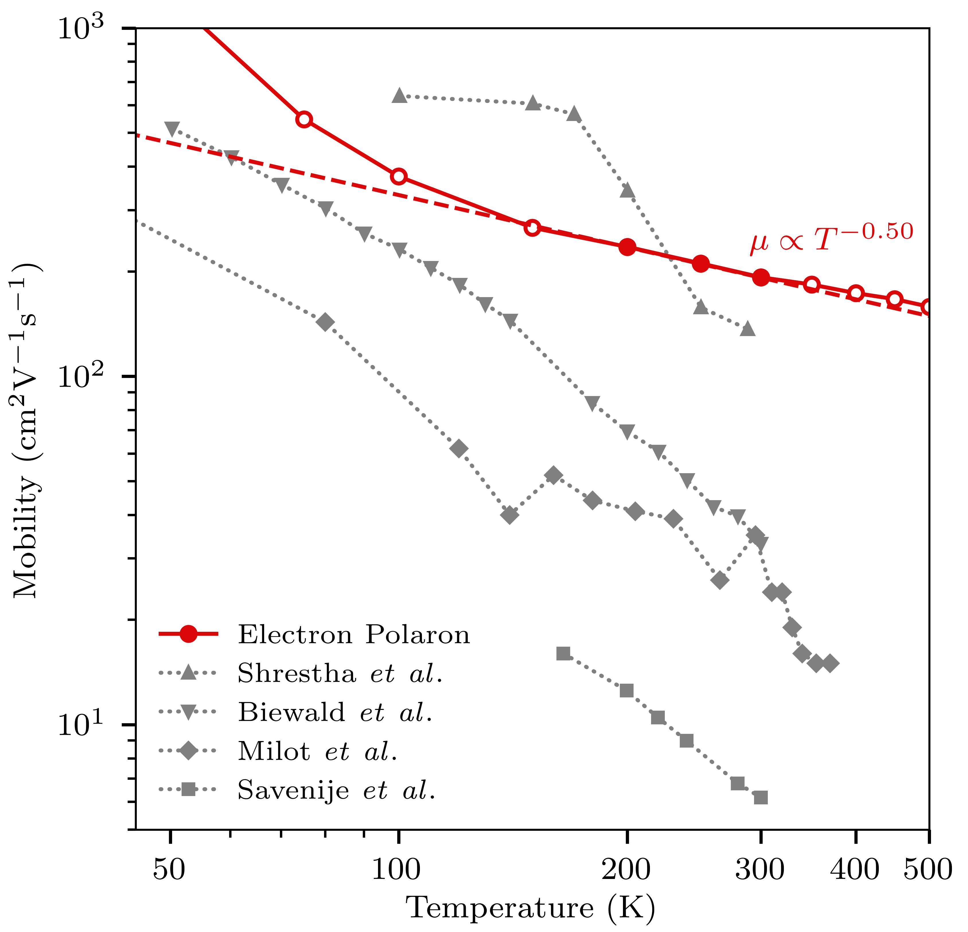
Figure 1: Temperature dependent mobilities of electron polarons in MAPbI₃ associated with material parameters found to minimise the polaron mobility temperature exponent (see Table 1). Solid red points show mobilities used during optimisation; open red points show mobilities calculated after optimisation to confirm exponential temperature dependence (for $T\geq 200K$). Errors in the mobility ensemble average are comparable to the data point size. Experimental data points are shown in grey with the symbols shown in the legend and are linked by dashed lines: Shrestha [30], Biewald [31], Milot [19], Savenije [18].

Using the approach described in section 3, 1269 simulations were required from 423 points (including initial set) in the 6-D simulation input parameter space at temperatures $200$K, $250$K and $300$K. The minimum temperature exponent of polaron mobility in MAPbI₃ was found to be $-0.50\pm 0.04$. This prediction resulted from optimisation in the hypervolume of input space defined by the uncertainty in each of the six material simulation input parameters. The optimisation procedure was terminated due to Gaussian Process Regression (GPR) predicting the probability of obtaining a temperature exponent equal to or more negative than $-1.5$ of $\sim 10^{-24}$. Table 1 shows the material parameters associated with the minimum temperature exponent found during minimisation. All material parameters lie within the assumed uniform uncertainty, except the effective mass $m^{*}$ which was found to minimise the temperature exponent at 0.12 $m_{e}$ (bottom of uncertainty range). This suggests that the temperature exponent may be further minimised by decreasing $m^{*}$. On increasing the prior uncertainty range to $\pm 40\%$ and allowing the minimisation procedure to continue, it was found that the temperature exponent may be further minimised to $-0.54$ with $m^{*}=0.098m_{e}$. This value of $m^{*}$ is well within the $\pm 40\%$ range, indicating that the temperature exponent may not be further minimised by decreasing $m^{*}$ (within this range). Additionally, a temperature exponent of $-0.54$ is within one standard error of the temperature exponent found within the $\pm 20\%$ uncertainty range and therefore does not affect any conclusions drawn below. Finally, increasing the material parameter uncertainty range to $\pm 40\%$ also leads to material parameters that are un-physical for MAPbI₃ (see [22, 14, 16, 28]).

An accurate prediction of the probability of reproducing a temperature exponent of $-1.5$ relies strongly on the accuracy of the output variance predicted by GPR. A measure of this accuracy is easily obtained and is described as follows. In the 6-D simulation input space, $100$ points were randomly generated and the temperature exponent of the polaron mobility calculated. Using the trained Gaussian Process Regressor, the predicted normal distribution (see Equation 3) over the temperature exponent for the $100$ points in input space was determined and $\pm 2\sigma,\pm 3\sigma$ $(95.5\%,99.7\%)$ confidence bounds were calculated. $88\%$ of simulated temperature exponents, for the $100$ points in input space, fell within $95.5\%$ predicted bounds, with $100\%$ of simulated temperature exponents within $99.7\%$ bounds. This indicates that the uncertainty of the GP (Gaussian Process) model is reasonably accurate and does not require further uncertainty calibration [34].

The accuracy of predicted GP model uncertainties provides strong evidence that the probability of obtaining a temperature exponent more negative than $-1.5$ is indeed vanishingly small, $\sim 10^{-24}$. Therefore, this modelling indicates that polaron formation in MAPbI₃ cannot explain the observed temperature dependence of electron mobility, even once the effect of a large uncertainty in the material simulation input parameters is considered. Other mechanisms that regulate charge-carrier dynamics in MAPbI₃ must be investigated, such as trapping and recombination, as polaron formation has been shown to be more limited in its effect on electron mobilities than previously hypothesised in the literature [20, 23, 24].

Table 1: Material parameters for electrons in MAPbI₃. Mean values sourced from ab initio calculations reported in the literature and summarised in reference [38]. Also shown are parameter values associated with the minimum discrepancy found during optimisation between the temperature exponent calculated from simulation and an experimental exponent of $-1.5$. Here m_e is electron mass, $\varepsilon_{0}$ vacuum electric permittivity.

Parameter	Mean value	Minimum exponent discrepancy value
Conduction band effective mass $m^{*}$	0.15 $m_{e}$	0.12 $m_{e}$
Polar optical phonon frequency $\omega_{\mathrm{pop}}/2\pi$	2.25 THz	2.67 THz
Low frequency permittivity $\varepsilon_{\mathrm{LF}}$	25.7 $\varepsilon_{0}$	27.1 $\varepsilon_{0}$
High frequency permittivity $\varepsilon_{\mathrm{HF}}$	4.5 $\varepsilon_{0}$	5.4 $\varepsilon_{0}$
Acoustic deformation potential $\Xi$	2.13 eV	1.7 eV
Elastic constant $c_{\mathrm{L}}$	32 GPa	32 GPa

2.2 Band electron and polaron mobility at 298K

Additionally, GPR was fit to both the band electron and polaron mobility as a function of the 6-D simulation input space at 298K, with mobilities calculated as described in section 3.2. A training set of 1000 simulations was obtained from randomly generated sets of simulation input parameters and their calculated band electron and polaron mobilities. A mean absolute percentage error of $0.5\%$ was achieved for both model predictions of band electron and polaron mobility on an unseen test set of 200 simulations. The trained length-scales of the covariance function of the GP for the two models provide information regarding the physical scattering mechanisms present in MAPbI₃. Specifically, a measure of the sensitivity of the band electron and polaron mobility to each of the six input parameters (normalised by removing mean and scaling to unit variance) is quantified by the inverse of the length-scale for each parameter (see Figure 2) [36].

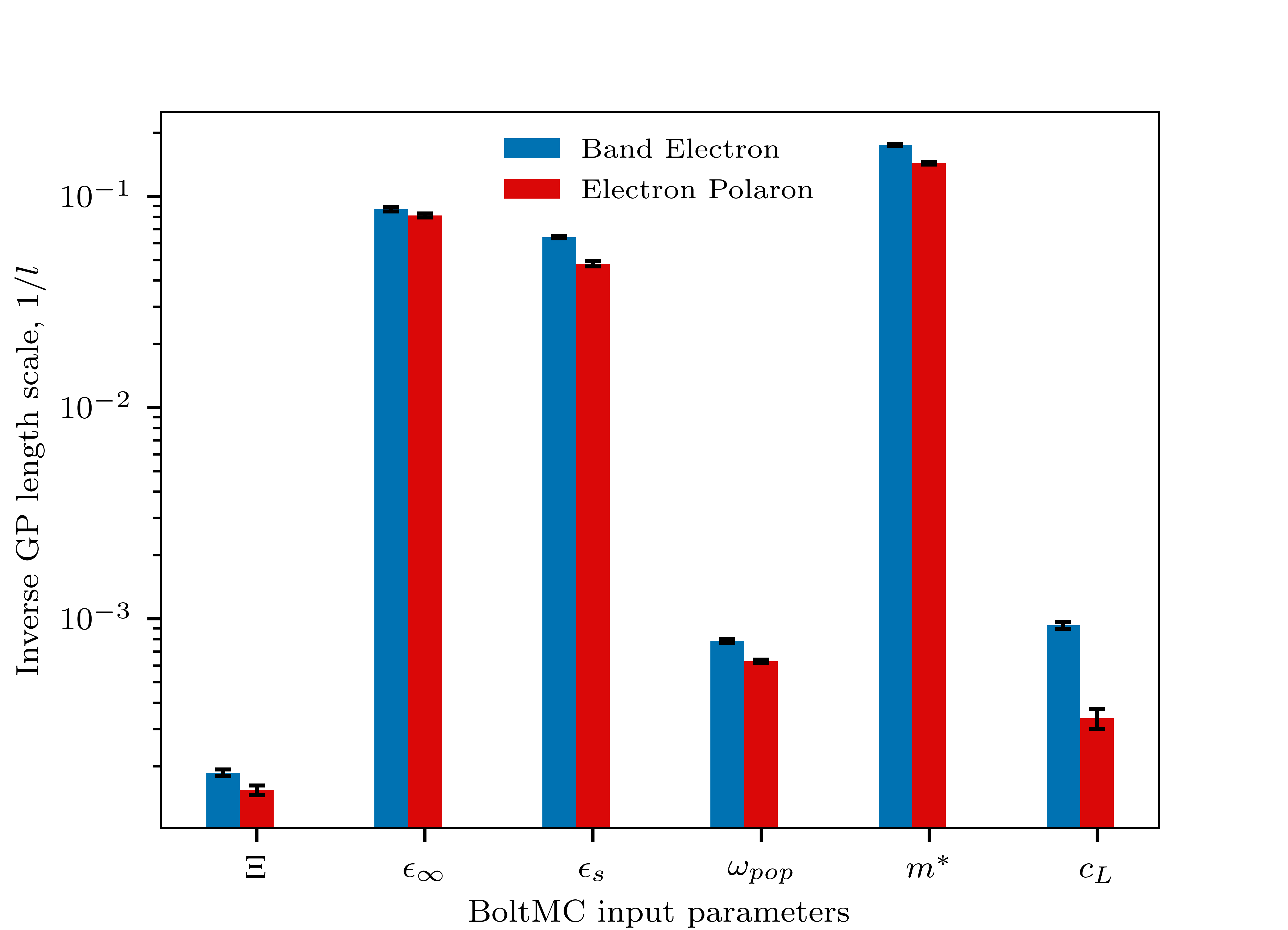
Figure 2: The inverse length-scales of covariance function (RBF) for each simulation input parameter, defined by mean values in Table 1, taken from two trained GPs predicting band electron and polaron mobility from simulation input parameters at 298K. The inverse length-scales are plotted such that larger values indicate larger output (mobility) sensitivity to that parameter. Error bars show standard error in the mean in black and were calculated by 10-fold cross validation over the training set.

An understanding of the effect of a small perturbation to an input parameter on the band electron and polaron mobility is therefore obtained, here providing insight into the physical mechanisms controlling polaron mobility in lead-halide perovskites. For MAPbI₃, this analysis suggests that the polaron mobility is less sensitive to a perturbation in any input parameter than seen for bare band electron mobility. Given the six input parameters define the polaron scattering rates for acoustic phonons, optical phonons and ionised impurities [38], this in turn suggests that the polaron mobility is less sensitive to perturbations in the scattering rates.

Furthermore, comparison across the magnitude of length-scales for each parameter (note that comparison between length-scales for different parameters is possible only as the input data was normalised before fitting GPR) indicate which perturbed scattering rates the electron mobility is most sensitive to, within the uncertainty in each input parameter. For example, a perturbation in the conduction band effective mass $m^{*}$ has the largest influence on the mobility. This can be rationalised from simple Drude theory $\mu=\tau(m^{*})/m^{*}$, where the mobility is mediated by the magnitude of $m^{*}$ directly as well as implicitly through the relaxation time $\tau(m^{*})$, arising from the dependence of the scattering rates on $m^{*}$. The effective mass can be seen to strongly regulate electron mobility, a result that is confirmed by this analysis.

Large mobility sensitivity to both low and high frequency permittivity, $\epsilon_{s}$ and $\epsilon_{\infty}$, is indicated by large inverse length-scales for both parameters. This suggests that the band electron/polaron mobility in MAPbI₃ has increased sensitivity to a perturbation in scattering rates strongly dependent on these parameters; namely, the scattering rates for polar optical phonons and ionised impurities due to their functional dependence on $(1/\epsilon_{\infty}-1/\epsilon_{s})$ and $1/\epsilon_{s}^{2}$, respectively [6]. Walsh [40] discussed the importance of dielectric screening for defect tolerance of perovskites, and, we infer, to charge transport. While, despite the dependence of the acoustic phonon scattering rate on $\Xi^{2}$ and $1/c_{L}$, the mobility sensitivity (inverse length-scale) to each parameter ($\Xi$, $c_{L}$) remains low - suggesting that a perturbation in the acoustic phonon scattering rate has a reduced effect on the band electron mobility. This effect on mobility is significantly decreased for polarons, indicated by the smaller inverse length-scale. Indeed, previous studies of polaron formation in MAPbI₃ have concluded that scattering due to acoustic phonons is the mechanism most significantly decreased in comparison to bare band electrons [38], a result confirmed by this analysis.

However, one must be careful in the physical insight derived from an analysis of the input parameter length-scales. Specifically, it is not clear that an input parameter with a larger length-scale has reduced significance in determining the band electron/polaron mobility; only that a perturbation in the parameter, and therefore perturbation in the scattering rate, has a smaller effect on the mobility. For example, it may be found that the magnitude of electron mobility is not significantly changed with a perturbation in one scattering rate. Yet this does not mean that electron mobility would be unchanged if this scattering mechanism was not present in the simulation, only that its contribution to the mobility is approximately constant over the range that the material parameters were varied.

Finally, this analysis is useful for guiding future uncertainty reduction, whereby reducing uncertainty in input parameters with smaller length scales will result in a greater decrease in the uncertainty over the simulation output. Similarly, an analysis of the length-scale for each input parameter may be used to determine a reduction in dimensionality of the simulation input space, by excluding parameters with comparatively large length-scales, in turn improving the efficiency of search/optimisation methods.

3 Methods

3.1 Efficient simulation input space search

Global optimisation of an expensive-to-evaluate ’black box’ function is a common problem across many disciplines [12]. Here, the ’black box’ function refers to a numerical simulation of a parameterized physical model. Bayesian Optimisation [13, 41] is frequently used in this setting and utilises a learned probabilistic model of the function that is being optimised. No knowledge of the functional form is assumed - e.g. the function is not assumed to be convex and gradients are not directly accessible. GPR has been used to model the functional relationship between the simulation input parameters $\mathbf{x}$ and output $g(\mathbf{x})$. GPs [11] can be viewed as specifying a distribution over functions,

$$g(\mathbf{x})\sim\mathcal{GP}(m(\mathbf{x}),k(\mathbf{x},\mathbf{x^{\prime}})),$$ (1)

where $m(\mathbf{x})$ defines the mean function and $k(\mathbf{x},\mathbf{x^{\prime}})$ the covariance function of the GP. The radial basis function (RBF) was used in this work to calculate $k(\mathbf{x},\mathbf{x^{\prime}})$, specifying the $i$’th row and $j$’th column of the covariance matrix with the addition of additive noise along the diagonal,

$$k(\mathbf{x}_{i},\mathbf{x}_{j})=\sigma_{f}^{2}\exp\Big(-\frac{|\mathbf{x}_{i}-\mathbf{x}_{j}|^{2}}{2l^{2}}\Big{missing})+\sigma_{n}^{2}\delta_{ij}.$$ (2)

The free parameters of the RBF, $\sigma_{f}^{2}$ and $l$, define the output signal variance and input length-scales respectively and $\sigma_{n}^{2}$ specifies the variance of additional Gaussian measurement noise. These parameters are optimised during training to maximise the log-marginal likelihood of the data. he choice of covariance function quantifies certain modelling assumptions that the underlying numerical function is expected to obey, such as smoothness, non-stationarity and periodicity [15]. The RBF kernel encodes a prior assumption that the output of the function to be approximated smoothly varies with respect to function input parameters.

For a GP, the predicted marginal distribution of any single function value $y$ (simulation output) is univariate normal [11]

$$p(y|\mathbf{x})=\mathcal{N}(y;\mu,\sigma^{2}),\hskip 14.22636pt\mu=m(\mathbf{x}),\hskip 14.22636pt\sigma^{2}=k(\mathbf{x},\mathbf{x}).$$ (3)

Bayesian Optimisation utilises this predicted distribution by determining the optimal next input location with which to query the ground truth function (here, simulation model), such that the probability of finding an optimum is maximised. Specifically, an acquisition function $\alpha(\mathbf{x})$ is defined over the input space and the next input location with which to query the ground truth function is determined by maximising this acquisition function,

$$\mathbf{x}_{n+1}=\arg\max_{\mathbf{x}}\alpha(\mathbf{x}).$$ (4)

Here, the acquisition function is defined by the probability of improvement (PI), and if minimisation of the ground truth function is desired, is given by [11]

$$\alpha(\mathbf{x})=P(g(\mathbf{x})\leq g(\mathbf{x}^{+})-\kappa),$$ (5)

where $\mathbf{x}^{+}$ represents the input location associated with the minimum function value observed thus far during optimisation and $\kappa$ is a hyper-parameter that defines the exploration-exploitation trade-off of the optimisation policy.

In this application, the function minimised during optimisation is the absolute value of the difference between predicted simulation output and the experimental result. The optimisation procedure can be terminated once either a simulation output is found that reproduces the experimental result below a pre-specified error, or the probability of obtaining an output equal to the experimental result falls below a threshold. This probability can be explicitly evaluated from predicted variance of the simulation output from GPR at each point in the input space; a method for determining the accuracy of the predicted variances is reported in section 3. Note that the probability of reproducing the experimental result may increase or decrease on the addition of a further simulation. The threshold probability must therefore be defined conservatively (i.e. sufficiently low) to avoid incorrect early stopping and/or performing a minimum number of iterations before terminating due to low probability.

3.2 Simulation of polaron dynamics

To demonstrate this method, polaron dynamics were simulated by solving an augmented form of Kadanoff’s semiclassical Boltzmann transport equation [2] using the ensemble Monte Carlo method [6, 3]. For an ensemble of polarons subject to a constant electric field $\mathbf{E}$, the Boltzmann transport equation is given by

$$\frac{\partial f}{\partial t}-\frac{e}{\hbar}\mathbf{E}\cdot\frac{\partial f}{\partial\mathbf{k}}=\Big{(}\frac{\partial f}{\partial t}\Big{)}_{pop}+\Big{(}\frac{\partial f}{\partial t}\Big{)}_{aco}+\Big{(}\frac{\partial f}{\partial t}\Big{)}_{imp},$$ (6)

where $\mathbf{k}$ is the polaron wavevector and $f(\mathbf{k},t)$ defines the one-particle distribution function. The partial derivatives on the right hand side of Equation (6) represent the change to the distribution function due to the scattering of polarons by optical phonons (pop), acoustic phonons (aco), and ionised impurities (imp). The scattering rates for each of these three mechanisms were calculated using Fermi’s golden rule,

$$S(\mathbf{k}_{i}\rightarrow\mathbf{k}_{j})=\frac{2\pi}{\hbar}|\bra{\mathbf{k}_{f}}H^{\prime}\ket{\mathbf{k}_{i}}|^{2}\delta(\epsilon_{f}-\epsilon_{i}-\Delta\epsilon),$$ (7)

where $H^{\prime}$ is the time-dependent perturbing Hamiltonian for each scattering mechanism in the bulk of a polar semiconductor [6]. $\epsilon_{i}$, $\epsilon_{f}$ are the energies of the initial and final states respectively and $\Delta\epsilon$ represents the quanta of energy exchanged as a result of the scattering. A derivation of the scattering rates for the three scattering mechanisms considered here for both band electrons and polarons can be found in [38].

Calculation of the scattering rates requires the polaron eigenstates $\ket{\mathbf{k}}$. These eigenstates were obtained from the Feynman model of a polaron where an electron is coupled to a second particle via a harmonic potential that represents the cloud of virtual phonons associated with the surrounding polarised ionic lattice [1]. The Hamiltonian of this system is given by [2]

$$\begin{split}H_{F}&=\frac{\hbar^{2}|\mathbf{k_{e}}|^{2}}{2m_{e}^{*}}+\frac{\hbar^{2}|\mathbf{k}_{c}|^{2}}{2m_{c}^{*}}+\frac{1}{2}\kappa(\mathbf{r}-\mathbf{r}_{c})^{2}\\ &=\frac{\hbar^{2}|\mathbf{k}|^{2}}{2m^{*}}+\hbar\omega_{osc}\sum_{i=1}^{3}\Big{(}(a_{osc})_{i}^{\dagger}(a_{osc})_{i}+\frac{1}{2}\Big{)}\end{split}$$ (8)

where $\mathbf{r},\mathbf{k}$ and $m^{*}$ are the position, wavevector and effective mass for the electron (subscript ’e’), phonon cloud (subscript ’c’) and polaron (no subscript). The polaron’s internal harmonic oscillator state is defined by the angular frequency $\omega_{osc}$, with $(a_{osc})_{i}^{\dagger}$ and $(a_{osc})_{i}$ representing the ladder operators for this harmonic oscillator system for the three cartesian directions, indexed by $i$.

Finally, steady-state solutions to the Boltzmann transport equation were obtained by the ensemble Monte Carlo method [6, 3] (additional information of this calculation and its computational implementation can be found in [38]) and the polaron mobility $\mu$ determined from the ensemble average of the polaron wavevector,

$$\mu=\frac{\hbar|\mathbf{\overline{k}|}}{|\mathbf{E}|m^{*}}.$$ (9)

Band electron dynamics were also simulated and the mobility calculated as described above but with the band electron state $\mathbf{k_{e}}$ determined from the effective mass Hamiltonian,

$$H_{0}=\frac{\hbar^{2}|\mathbf{k_{e}}|^{2}}{2m_{e}^{*}}.$$ (10)

3.3 Polaron dynamics under input uncertainty

To calculate the polaron scattering rates, six material parameters were required that define the semiconductor to be simulated and can be viewed as specifying a 6-D input space. These parameters for MAPbI₃, as predicted by electronic structure calculations, can be seen in Table 1. The uncertainty in each of the six MAPbI₃ input parameters was assumed to be $\pm 20\%$, in the absence of uncertainty estimation accompanying ab initio prediction [38]. This assumed uncertainty results in input parameter values that align with values presented in a range of previous studies, both theoretical predictions and experimental measurements [22, 14, 16, 28]. In the hypervolume of the 6-D input space defined by the uncertainty in each input parameter, $300$ points (sets of input parameters) were randomly generated and the polaron mobility calculated at $200$K, $250$K and $300$K. The temperature dependence of the polaron mobility has been characterised by fitting the power-law relationship,

$$\mu(T)=\mu_{0}T^{\beta}$$ (11)

where $\beta$ is the temperature exponent obtained from the gradient of a linear fit performed on log-log axes,

$$\log(\mu(T))=\log(\mu_{0})+\beta\log(T).$$ (12)

The temperature exponent $\beta$ was used as the predicted variable $y$ for GPR, as a function of the 6-D input space $\mathbf{x}$. As noted in section 3.1, Bayesian Optimisation could then be used to minimise the absolute value of the difference between the predicted temperature exponent and an experimentally measured exponent of $-1.5$ (see Figure 1). The Python codes used for performing this procedure, with the supporting data used to run the code, can be found in [43]. Correlations between input parameters have not been considered during optimisation as constraining the optimisation procedure by considering parameter correlations would only decrease the searched parameter space. In this specific application, reducing the searched parameter space may result in a temperature exponent optimum further from the experimental exponent but never closer (as the space considered is inclusive of the correlation constrained space). While any correlations between input parameters will be important in other applications, their inclusion here would not affect any conclusions drawn.

4 Conclusions

We have demonstrated that Bayesian Optimisation can efficiently search a region of the simulation input space defined by the uncertainty in each input parameter to minimise the difference between the simulation output and a set of experimental results. This was achieved through explicit evaluation of the probability that the simulation can reproduce the measured experimental results in this region of input space. With this method, 1269 simulations using the code BoltMC were required from 423 points in the 6-D simulation input parameter space (three temperatures at each point in input space). A naive grid search of any simulation input space would require $n^{d}$ points, for $n$ discrete parameter values along each input dimension $d$, rendering a quantification of input uncertainty computationally intractable for most numerical physics simulations. Here, a coarse grid ($n=10$) would require $2\times 10^{6}$ simulations. Given the generality of the method, application to other numerical simulations (in semiconductor physics and other fields) is straightforward. For physical models known to exhibit a non-linear functional dependence on model inputs, this method allows for more complete conclusions to be drawn from results as the effect of input parameter uncertainty on the simulation output has been determined.

The minimum temperature exponent of the polaron mobility found during optimisation was $-0.50\pm 0.04$, with the probability of reproducing an experimental exponent of $-1.5$ found to be $\sim 10^{-24}$. This result suggests that the formation of large polarons in MAPbI₃ cannot explain the observed temperature dependence of electron mobility; other mechanisms that regulate charge-carrier dynamics in lead-halide perovskites, such as trapping and recombination, must therefore be investigated.

Additionally, with analysis of the length-scales of the covariance function for GPR, polaron mobility was found to be less sensitive to perturbations in the scattering rates than observed for band electrons. Both band electrons and polarons in MAPbI₃ displayed greater mobility sensitivity to perturbations in the scattering rates for polar optical phonons and ionised impurities, with the effect on mobility of a perturbation in the acoustic phonon scattering rate significantly decreased.

Data Availability

Data that supports the findings of this study is available within the article. The article has no supplementary material. The code with supporting data for this article is publicly available at https://github.com/sammccallum/BoltMC-Bayes-Opt where the datasets and code files are described in README.md.

References

- [1] R.. Feynman “Slow Electrons in a Polar Crystal” In Phys. Rev. 97 American Physical Society, 1955, pp. 660–665 DOI: 10.1103/PhysRev.97.660
- [2] Leo P. Kadanoff “Boltzmann Equation for Polarons” In Phys. Rev. 130 American Physical Society, 1963, pp. 1364–1369 DOI: 10.1103/PhysRev.130.1364
- [3] W. Fawcett, A.D. Boardman and S. Swain “Monte Carlo determination of electron transport properties in gallium arsenide” In Journal of Physics and Chemistry of Solids 31.9, 1970, pp. 1963–1990 DOI: https://doi.org/10.1016/0022-3697(70)90001-6
- [4] Ken’ichi Okamoto and Shigeo Takeda “Polaron Mobility at Finite Temperature in the Case of Finite Coupling” In Journal of the Physical Society of Japan 37.2, 1974, pp. 333–339 DOI: 10.1143/JPSJ.37.333
- [5] R. Car and M. Parrinello “Unified Approach for Molecular Dynamics and Density-Functional Theory” In Phys. Rev. Lett. 55 American Physical Society, 1985, pp. 2471–2474 DOI: 10.1103/PhysRevLett.55.2471
- [6] C. Jacoboni and P. Lugli “The Monte Carlo Method for Semiconductor Device Simulation” Springer Vienna, 1989
- [7] M.. Payne et al. “Iterative minimization techniques for ab initio total-energy calculations: molecular dynamics and conjugate gradients” In Rev. Mod. Phys. 64 American Physical Society, 1992, pp. 1045–1097 DOI: 10.1103/RevModPhys.64.1045
- [8] J. Oakley and A. O’Hagan “Bayesian inference for the uncertainty distribution of computer model outputs” In Biometrika 89, 2002, pp. 769–784
- [9] J. Oakley and A. O’Hagan “Probabilistic sensitivity analysis of complex models: A Bayesian approach” In J. Royal Statistical Society, Series B 66, 2004, pp. 751–769
- [10] A. O’Hagan “Bayesian analysis of computer code outputs: A tutorial” The Fourth International Conference on Sensitivity Analysis of Model Output (SAMO 2004) In Reliability Engineering & System Safety 91.10, 2006, pp. 1290–1300 DOI: https://doi.org/10.1016/j.ress.2005.11.025
- [11] Carl Edward Rasmussen and Christopher K.. Williams “Gaussian Processes for Machine Learning” MIT Press, 2006
- [12] Songqing Shan and Gary Wang “Survey of modeling and optimization strategies to solve high-dimensional design problems with computationally-expensive black-box functions” In Structural and Multidisciplinary Optimization 41, 2010, pp. 219–241 DOI: 10.1007/s00158-009-0420-2
- [13] Jasper Snoek, Hugo Larochelle and Ryan P. Adams “Practical Bayesian Optimization of Machine Learning Algorithms” arXiv, 2012 DOI: 10.48550/ARXIV.1206.2944
- [14] Federico Brivio, Alison B. Walker and Aron Walsh “Structural and electronic properties of hybrid perovskites for high-efficiency thin-film photovoltaics from first-principles” In APL Mater 1, 2013, pp. 042111 DOI: https://doi.org/10.1063/1.4824147
- [15] Andrew Gelman et al. “Bayesian Data Anlysis” CRC Press, 2013
- [16] Federico Brivio, Keith T. Butler, Aron Walsh and Mark Schilfgaarde “Relativistic quasiparticle self-consistent electronic structure of hybrid halide perovskite photovoltaic absorbers” In Phys. Rev. B 89 American Physical Society, 2014, pp. 155204 DOI: 10.1103/PhysRevB.89.155204
- [17] M. Green, A. Ho-Baillie and H. Snaith “The emergence of perovskite solar cells.” In Nature Photon 8, 2014, pp. 506–514 DOI: https://doi.org/10.1038/nphoton.2014.134
- [18] Tom J. Savenije et al. “Thermally Activated Exciton Dissociation and Recombination Control the Carrier Dynamics in Organometal Halide Perovskite” In The Journal of Physical Chemistry Letters 5.13, 2014, pp. 2189–2194 DOI: 10.1021/jz500858a
- [19] Rebecca L. Milot et al. “Temperature-Dependent Charge-Carrier Dynamics in CH3NH3PbI3 Perovskite Thin Films” In Advanced Functional Materials 25.39, 2015, pp. 6218–6227 DOI: https://doi.org/10.1002/adfm.201502340
- [20] X.-Y. Zhu and V. Podzorov “Charge Carriers in Hybrid Organic–Inorganic Lead Halide Perovskites Might Be Protected as Large Polarons” In The Journal of Physical Chemistry Letters 6.23, 2015, pp. 4758–4761 DOI: 10.1021/acs.jpclett.5b02462
- [21] Stefano Razza, Sergio Castro-Hermosa, Aldo Di Carlo and Thomas M. Brown “Research Update: Large-area deposition, coating, printing, and processing techniques for the upscaling of perovskite solar cell technology” In APL Materials 4.9, 2016, pp. 091508 DOI: 10.1063/1.4962478
- [22] Jarvist Moore Frost “Calculating polaron mobility in halide perovskites” In Phys. Rev. B 96 American Physical Society, 2017, pp. 195202 DOI: 10.1103/PhysRevB.96.195202
- [23] Kanatzidis M. al. Mante PA. “Electron–acoustic phonon coupling in single crystal CH3NH3PbI3 perovskites revealed by coherent acoustic phonons.” In Nat. Commun. 8, 2017, pp. 195203 DOI: https://doi.org/10.1038/ncomms14398
- [24] Mingliang Zhang et al. “Charge transport in hybrid halide perovskites” In Phys. Rev. B 96 American Physical Society, 2017, pp. 195203 DOI: 10.1103/PhysRevB.96.195203
- [25] David A. Egger et al. “What Remains Unexplained about the Properties of Halide Perovskites?” In Advanced Materials 30.20, 2018, pp. 1800691 DOI: https://doi.org/10.1002/adma.201800691
- [26] Laura M. Herz “How Lattice Dynamics Moderate the Electronic Properties of Metal-Halide Perovskites” In The Journal of Physical Chemistry Letters 9.23, 2018, pp. 6853–6863 DOI: 10.1021/acs.jpclett.8b02811
- [27] S. Jenatsch et al. “Quantitative analysis of charge transport in intrinsic and doped organic semiconductors combining steady-state and frequency-domain data” In Journal of Applied Physics 124.10, 2018, pp. 105501 DOI: https://doi.org/10.1063/1.5044494
- [28] Jung-Hoon Lee et al. “The competition between mechanical stability and charge carrier mobility in MA-based hybrid perovskites: insight from DFT” In J. Mater. Chem. C 6 The Royal Society of Chemistry, 2018, pp. 12252–12259 DOI: 10.1039/C8TC04750B
- [29] Martin Schlipf, Samuel Poncé and Feliciano Giustino “Carrier Lifetimes and Polaronic Mass Enhancement in the Hybrid Halide Perovskite from Multiphonon Fröhlich Coupling” In Phys. Rev. Lett. 121 American Physical Society, 2018, pp. 086402 DOI: 10.1103/PhysRevLett.121.086402
- [30] Shreetu Shrestha et al. “Assessing Temperature Dependence of Drift Mobility in Methylammonium Lead Iodide Perovskite Single Crystals” In The Journal of Physical Chemistry C 122.11, 2018, pp. 5935–5939 DOI: 10.1021/acs.jpcc.8b00341
- [31] Alexander Biewald et al. “Temperature-Dependent Ambipolar Charge Carrier Mobility in Large-Crystal Hybrid Halide Perovskite Thin Films” In ACS Applied Materials & Interfaces 11.23, 2019, pp. 20838–20844 DOI: 10.1021/acsami.9b04592
- [32] Otten S. al. Caron S. “Constraining the parameters of high-dimensional models with active learning.” In Eur. Phys. J. 79, 2019, pp. 944 DOI: 10.1140/epjc/s10052-019-7437-5
- [33] A.. Jena, A. Kulkarni and T. Miyasaka “Halide Perovskite Photovoltaics: Background, Status, and Future Prospects” In Chem Rev. 13, 2019, pp. 3036–3103 DOI: 10.1021/acs.chemrev.8b00539
- [34] A. Kumar, P.S Liang and T. Ma “Verified Uncertainty Calibration” In Advances in Neural Information Processing Systems 32 (NeurIPS 2019), 2019 URL: https://papers.nips.cc/paper_files/paper/2019
- [35] Martin T. Neukom et al. “Consistent Device Simulation Model Describing Perovskite Solar Cells in Steady-State, Transient, and Frequency Domain” In ACS Applied Materials & Interfaces 11.26, 2019, pp. 23320–23328 DOI: 10.1021/acsami.9b04991
- [36] Topi Paananen, Juho Piironen, Michael Riis Andersen and Aki Vehtari “Variable selection for Gaussian processes via sensitivity analysis of the posterior predictive distribution” In Proceedings of the Twenty-Second International Conference on Artificial Intelligence and Statistics 89, Proceedings of Machine Learning Research PMLR, 2019, pp. 1743–1752 URL: https://proceedings.mlr.press/v89/paananen19a.html
- [37] S. Jenatsch, S. Züfle, B. Blülle and B. Ruhstaller “Combining steady-state with frequency and time domain data to quantitatively analyze charge transport in organic light-emitting diodes” In Journal of Applied Physics 127.3, 2020, pp. 031102 DOI: https://doi.org/10.1063/1.5132599
- [38] Lewis A.. Irvine, Alison B. Walker and Matthew J. Wolf “Quantifying polaronic effects on the scattering and mobility of charge carriers in lead halide perovskites” In Phys. Rev. B 103 American Physical Society, 2021, pp. L220305 DOI: 10.1103/PhysRevB.103.L220305
- [39] Evelyne Knapp et al. “XGBoost Trained on Synthetic Data to Extract Material Parameters of Organic Semiconductors” In 2021 8th Swiss Conference on Data Science (SDS), 2021, pp. 46–51 DOI: 10.1109/SDS51136.2021.00015
- [40] Aron Walsh “Concluding remarks: emerging inorganic materials in thin-film photovoltaics” In Faraday Discuss. 239 The Royal Society of Chemistry, 2022, pp. 405–412 DOI: 10.1039/D2FD00135G
- [41] Roman Garnett “Bayesian Optimization” Cambridge University Press, 2023
- [42] Kanishka Kobbekaduwa et al. “Ultrafast Carrier Drift Transport Dynamics in CsPbI3 Perovskite Nanocrystalline Thin Films” In ACS Nano 17.14, 2023, pp. 13997–14004 DOI: 10.1021/acsnano.3c03989
- [43] Samuel G. McCallum and James E. Lerpiniére “”sammccallum/BoltMC-Bayes-Opt””, 2023 URL: https://github.com/sammccallum/BoltMC-Bayes-Opt