Impact of architecture on robustness and interpretability of multispectral deep neural networks

Abstract

Including information from additional spectral bands (e.g., near-infrared) can improve deep learning model performance for many vision-oriented tasks. There are many possible ways to incorporate this additional information into a deep learning model, but the optimal fusion strategy has not yet been determined and can vary between applications. At one extreme, known as “early fusion,” additional bands are stacked as extra channels to obtain an input image with more than three channels. At the other extreme, known as “late fusion,” RGB and non-RGB bands are passed through separate branches of a deep learning model and merged immediately before a final classification or segmentation layer.

In this work, we characterize the performance of a suite of multispectral deep learning models with different fusion approaches, quantify their relative reliance on different input bands and evaluate their robustness to naturalistic image corruptions affecting one or more input channels.

1 INTRODUCTION

Many datasets of overhead imagery, in particular those collected by satellites, contain spectral information beyond red, blue and green (RGB) channels (i.e. visible light). With the development of new sensors and cheaper launch vehicles, the availability of such multispectral overhead images has grown rapidly in the last 5 years. Deep learning applied to RGB images is at this point a well-established field, but by comparison, the application of deep learning techniques to multispectral imagery is in a comparatively nascent state. From an implementation perspective, the availability of additional spectral bands expands the space of neural network architecture design choices, as there are a plethora of ways one might “fuse” information coming from different input channels. From an evaluation perspective, multispectral imagery provides a new dimension in which to study model robustness. While in a recent years there has been a large amount of research on robustness of RGB image models to naturalistic distribution shifts such as image corruptions, our understanding of the robustness of multispectral neural networks is still limited. Such an understanding will be quite valuable, as an honest assessment of the trustworthiness of multispectral deep learning models will allow for more informed decisions about deployment of these models in high-stakes applications and use of their predictions in downstream analyses.

We take a first step in this direction, studying multispectral models operating on RGB and near-infrared (NIR) channels on two different data sets and tasks (one involving image classification, the other image segmentation). In addition, for each dataset/task we consider two different multispectral fusion architectures, early and late (to be described below). Our findings include:

1. Even when different fusion architectures achieve near-identical performance as measured by test accuracy, they leverage information from the various spectral bands to varying degrees: we find that for classification models trained on a dataset of RGB+NIR overhead images, late fusion models place far more importance on the NIR band in their predictions than their early fusion counterparts.

2. In contrast, for segmentation models we observe that both fusion styles resulted in models that place greater importance on RGB channels, and this effect is more pronounced for late fusion models.

3. Perhaps unsurprisingly, these effects are mirrored in an evaluation of model robustness to naturalistic image corruptions affecting one or more input channels — in particular, early fusion classification models are more sensitive to corruptions of RGB inputs, and segmentation models with either architecture are comparatively immune to corruptions affecting NIR inputs alone.

4. On the whole, our experiments suggest that segmentation models and classification models use multispectral information in different ways.

2 RELATED WORK

The perceptual score metric discussed in section 4 was introduced in [1], and it can be viewed as a member of a broader family of model evaluation metrics based on “counterfactual examples.” For a (by no means comprehensive) sample of the latter, see [2, 3], and for some cautionary tales about the use of certain counterfactual inputs see [4].

For a look at the state of the art of machine learning model robustness, we refer to [5]. The work most directly related to this paper was the creation of the ImageNet-C dataset [6], obtained from the ImageNet [7] validation split by applying a suite of naturalistic image corruptions at varying levels of severity. The original ImageNet-C paper [6] showed that even state-of-the-art image classifiers that approach human accuracy on clean images suffer severe performance degradation on corrupted images (even those that remain easily recognizable to humans). More recent work [8] evaluated the corruption robustness image segmentation models, finding that their robust accuracy tends to be correlated with clean accuracy and that some architectural features have a strong impact on robustness. All of the research in this paragraph deals with RGB imagery alone.

There is a limited amount of work on robustness of multispectral models, and most of the papers we are aware of investigate adversarial robustness, i.e. robustness to worst case perturbations of images [9, 10, 11] generated by a hypothetical attacker exploiting the deep learning model in question. It is worth noting that there is a lively ongoing discussion about the realism of the often-alleged security threat posed by adversarial examples [12]. The only research we are aware of addressing robustness of multispectral deep learning models to naturalistic distribution shift is [13], which studies the robustness of land cover segmentation models evaluated on images with varying level of occlusion by clouds.

3 DATASETS, TASKS AND MODEL ARCHITECTURES

The RarePlanes dataset [14] includes 253 Maxar Worldview-3 satellite scenes including $\approx 15,000$ human annotated aircraft. Crucially for our purposes this data includes RGB, multispectral and panchromatic bands. In addition to bounding boxes identifying the locations of aircraft, annotations contain meta-data features providing information about each aircraft. Of particular interest is the role of an aircraft, for which the possible values are displayed in LABEL:tbl:role-feat.

Table 1: The RarePlanes role meta-data feature. Sub-attributes marked with $\ast$ have fewer than 10 training examples and are omitted from our classification dataset.

() Attribute	Sub-attribute
()
Civil	{Large, Medium, Small} Transport
Military	Fighter, Bomber,* Transport, Trainer*
()

Using this information, we create an RGB+NIR image classification data set with the following processing pipeline: beginning with the 8-band, 16-bit multispectral scenes, we apply pansharpening, rescaling from 16- to 8-bit, contrast stretching, and gamma correction (for further details see appendix A). This results in 8-band, 8-bit scenes, from which we obtain the RGB and NIR channels. To extract individual plane images or "chips" from the full satellite images, we clip the image around each plane using the bounding box annotations. We use the plane role sub-attributes (from the right column of LABEL:tbl:role-feat) as classification labels, and omit the "Military Trainer" and "Military Bomber" classes, which only have 15 and 6 examples, respectively. The remaining five classes have approximately 14,700 datapoints.

We create a train-test split at the level of full satellite images. Note that this this presumably results in a more challenging machine learning task (compared with randomly splitting after creating chips), since it requires a model to generalize to new geographic locations, azimuth and sun elevation angles, and weather. We further divide the training images into a training and validation split, and keep the test images for unseen, hold-out evaluations. The final data splits are spread 74%/13%/13% between training, validation, and test, with class examples as evenly distributed as possible. The RarePlanes data set also includes a large amount of synthetic imagery — however, the synthetic data only includes RGB imagery. Thus, in our experiments we only use the real data.

We train four different types of image classifiers on the RGB+NIR RarePlanes chips, all assembled from ResNet backbones [15]:

RGB

A standard ResNet34 operating on the RGB channels (NIR is ignored)

NIR

A ResNet34 operating on the NIR channel alone (RGB is ignored)

early fusion

RGB and NIR channels are concatenated to create a four channel input image, and passed into a 4 channel ResNet34

late fusion

RGB and NIR channels are passed into separate ResNet34 models, and the pentultimate hidden feature vectors of the respective models are concatenated — the concatenated feature factor is then passed to a final classification head.

The two fusion architectures are illustrated in fig. 1.

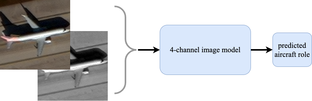
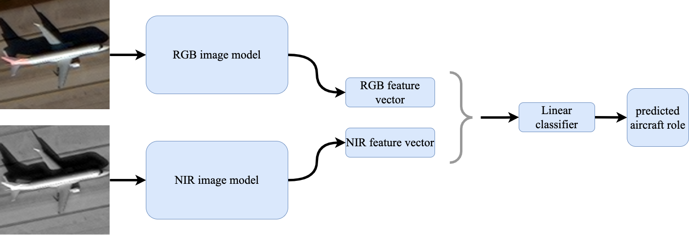
Figure 1: RGB+NIR fusion architectures. Top: early, Bottom: late. Braces denote image/feature concatenation.

We train these RarePlanes image classifiers using transfer learning: rather than beginning with randomly initialized weights, wherever possible we start with ResNet34 weights pre-trained on the ImageNet dataset [7], and then fine-tune with continued stochastic gradient descent to minimize cross entropy loss on RarePlanes. Notably, for models with NIR input, the first layer convolution weights are initialized with the Red channel weights trained on ImageNet. Further architecture, initialization and optimization details can be found in appendix B. All model accuracies lie in the range $91.8-92.5\%$.

We also use the Urban Semantic 3D (hereafter US3D) dataset [16, 17, 18, 19] of overhead 8-band, 16-bit multispectral images and LiDAR point cloud data with segmentation labels. The US3D segmentation labels consist of seven total classes, including ground, foliage, building, water, elevated roadway, and two "unclassified" classes, corresponding to difficult or bad pixels. From this data we create an image segmentation dataset via the following procedure: First, the 8-band, 16-bit multispectral images are converted to 8-bit RGB+NIR images with a pipeline similar to the one used for RarePlanes above. The resulting images are quite large, and are subdivided into 27,021 $1024\times 1024$ non-overlapping “tiles” with associated segmentation labels. Again, train/validation/test splits are created at the level of parent satellite images, and care is taken to ensure that the distributions of certain meta-data properties (location, view-angle and azimuth angle) are relatively similar from one split to the next. Further details can be found in appendix A.

Our segmentation models use the DeepLabv3 architecture [20]. To obtain neural networks taking both RGB and NIR images as inputs, we can apply the strategy described in fig. 1 to the backbone of DeepLabv3 (for a more detailed description of DeepLabv3’s components see appendix B). More precisely, we consider four different backbones:

RGB

A ResNet50 operating on the RGB channels (NIR is ignored)

NIR

A ResNet50 operating on the NIR channel alone (RGB is ignored)

early fusion

RGB and NIR channels are concatenated to create a four channel input image, and passed into a 4 channel ResNet50

late fusion

RGB and NIR channels are passed into separate ResNet50 models, and the resulting feature vectors of the respective models are concatenated — the concatenated feature factor is then passed to the DeepLabv3 segmentation head.

As in the case of our RarePlanes experiments, we fine-tune pre-trained weights, beginning with segmentation models pretrained on the COCO datatset [21] and again initializing both the first-layer R and NIR convolution weights with the R channel weights trained on COCO. In comparison to training the RarePlanes models, this optimization problem is far more computationally demanding, due to the larger tiles, larger networks and more challenging learning objective. We used (data parallel) distributed training on a cluster computer to scale batch size and reduce training and evaluation time. All model validation IoU scores lie in the range $0.53-0.55$ — for details and hyper parameters see appendix B.

4 PERCEPTUAL SCORES OF MULTISPECTRAL MODELS

Given a neural network processing multispectral (in our case RGB+NIR) images, one can ask is which bands the model is leveraging to make its predictions. More generally, we may want to know the relative importance of each spectral band for a given model prediction. This information is of potential interest for a number of reasons:

• For many objects of interest, reflectance properties vary widely between spectral bands (for example, plants appear vividly in the NIR band). Depending on the machine learning task and underlying data, this phenomenon could cause a multispectral model to prioritize one of its input channels.

• Some spectral bands are less affected by adverse weather or environmental conditions. For example, NIR light can penetrate haze, and NIR imagery is often used by human analysts to help discern detail in smoky or hazy scenes.

• In some applications, the different bands included in a multispectral dataset could have been captured by different sensors. For example, an autonomous vehicle may be equipped with an RGB camera and a thermal IR camera mounted side-by-side. In such a situation, technical issues affecting one sensor could result in image corruptions that only affect a subset of channels, and the performance of the downstream model predictions would depend on the relative importance of the corrupted channels.

A simple baseline for assessing the relative the importance of input channels for the predictions of a multispectral model is provided by the perceptual score metric [1], computed for RGB and NIR channels as follows: let $f(x_{\text{RGB}},x_{\text{NIR}})$ be an RGB+NIR model, where $x_{\text{RGB}}$ and $x_{\text{NIR}}$ denote the RGB and NIR inputs respectively. Let

$$\mathcal{D}=\{(x_{\text{RGB},i},x_{\text{NIR},i},y_{i})\,|\,i=1,\dots,N\}$$ (4.1)

be the test data set, where the $y_{i}$ are classification or segmentation labels, and let $\ell(f(x_{\text{RGB}},x_{\text{NIR}}),y)$ be the relevant accuracy function (0-1 loss for classification, Intersection-over-Union (IoU) for segmentation). The test accuracy of $f$ is then

$$\operatorname{Acc}(f,\mathcal{D})=\frac{1}{N}\sum_{i=1}^{N}\ell(f(x_{\text{RGB},i},x_{\text{NIR},i}),y_{i}).$$ (4.2)

To assess the importance of NIR information for model predictions, we use a counterfactual dataset

$$\mathcal{D}_{\text{NIR},\sigma}=\{(x_{\text{RGB},i},x_{\text{NIR},\sigma(i)},y_{i})\,|\,i=1,\dots,N\}$$ (4.3)

obtained by shuffling the NIR “column” of $\mathcal{D}$ with a random permutation $\sigma$ of $\{1,\dots,N\}$. In other words, the data points $(x_{\text{RGB},i},x_{\text{NIR},\sigma(i)},y_{i})$ consist of a labelled RGB image $(x_{\text{RGB},i},y_{i})$ together with the NIR channel $x_{\text{NIR},\sigma(i)}$ of some other randomly selected data point in $\mathcal{D}$. The perceptual score of the NIR input is then

$$\operatorname{PS}(f,\mathcal{D},\text{NIR},\sigma):=\frac{\operatorname{Acc}(f,\mathcal{D})-\operatorname{Acc}(f,\mathcal{D}_{\text{NIR},\sigma})}{\operatorname{Acc}(f,\mathcal{D})}.$$ (4.4)

In words, this is the relative accuracy drop incurred by evaluating $f$ on the dataset $\mathcal{D}_{\text{NIR},\sigma}$ — intuitively, if NIR input is important to $f$, replacing the NIR channel $x_{\text{NIR},i}$ with the NIR channel $x_{\text{NIR},\sigma(i)}$ of some other randomly chosen image will significantly damage the accuracy of $f$, resulting in a large relative drop in eq. 4.4.

The RGB perceptual score $\operatorname{PS}(f,\mathcal{D},\text{NIR},\sigma)$ is defined analogously, permuting the RGB column instead of the NIR. In practice, we average these metrics over several (e.g. 10) randomly selected permutations $\sigma$ of $\{1,\dots,N\}$, and henceforth $\sigma$ will be suppressed. In fact [1] defines two variants of perceptual score and refers to the one in eq. 4.4 as “model normalized”; their “task normalized” variant uses majority vote accuracy (i.e. accuracy of a naïve baseline) in the denominator instead of $\operatorname{Acc}(f,\mathcal{D})$. We include both score normalizations for completeness, but note that in all cases the normalization did not change our qualitative conclusions. Figure 2 displays these metrics for RarePlanes classifiers, and shows that from the perspective of perceptual score, early fusion models pay more attention to RGB channels whereas late fusion models pay more attention to NIR.

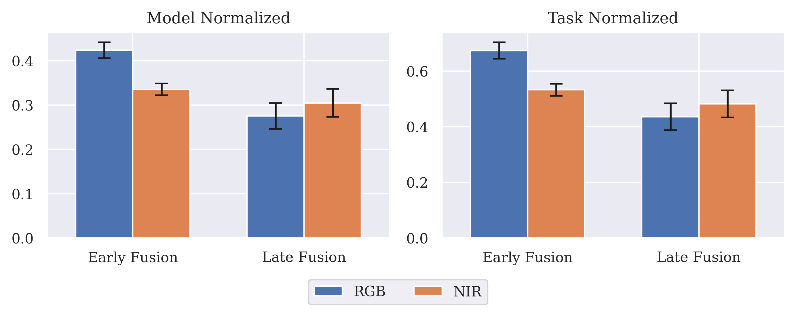
Figure 2: Perceptual scores for the RarePlanes multispectral classifiers. The early fusion models have a higher perceptual score for RGB channels (i.e., more reliance on RGB inputs), whereas the late fusion models have higher perceptual score for NIR channels (i.e., more reliance on NIR input). Error bars are obtained from five evaluations of the experiment with independent random number generator seeds.

There is a simple heuristic explanation for these results: for both model architectures, RGB channels occupy $75\%$ of the input space dimensions. In contrast, in the late fusion models the RGB and NIR inputs are both encoded as 512-dimensional feature vectors which are concatenated before being passed to the classification head (a 2 layer MLP); hence from the perspective of the classification head, RGB and NIR each account for half of the feature dimensions.

Our measurements of perceptual score for segmentation models on US3D, shown in fig. 3 are quite different: they suggest the late fusion model pays even less attention (again, from the perspective of perceptual score) to NIR

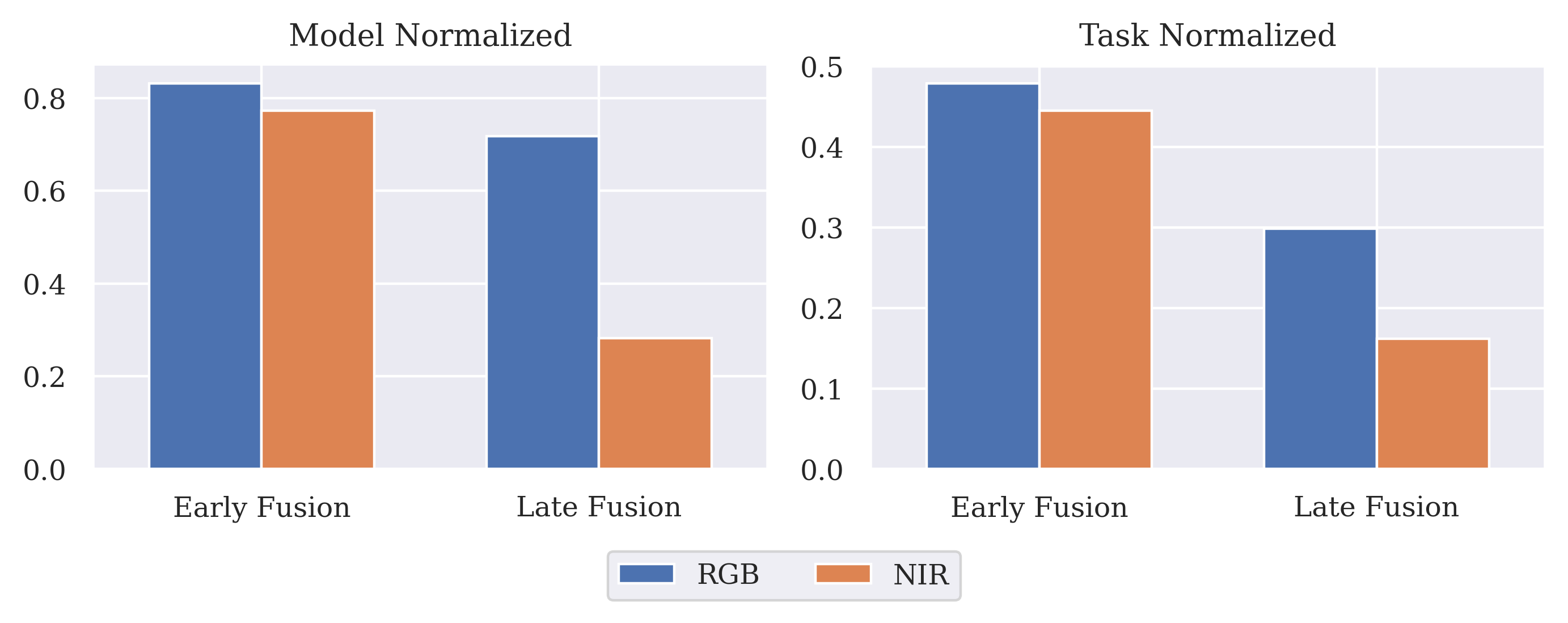
Figure 3: Perceptual scores for the US3D multispectral segmentation models. Both early and late fusion models have higher perceptual scores for RGB data, demonstrating that model performance relies more strongly on the RGB inputs. For late fusion models this effect is even more dramatic, suggesting that the NIR input is less important, in contrast to the classification model scores shown in fig. 2.

information than the early fusion model. This finding is in tension with both fig. 2 and the heuristic explanation thereof. One challenge encountered in interpreting fig. 3 is that due to the computational cost of training we only trained one model for each architecture. We leave a larger experiment allowing for estimation of statistical significance to future work.

5 ROBUSTNESS TO NATURALISTIC CORRUPTIONS

The perceptual scores presented in the previous section aim to quantify our models’ dependence on RGB and NIR inputs. A related question is how robust these models are to naturally occurring corruptions that affect either (or both) of the RGB or NIR inputs. With this in mind, we create corrupted variants of RarePlanes and US3D by applying a suite of image transformations simulating the effects of noise, blur, weather and digital corruptions. This is accomplished using a fork of the code that generated ImageNet-C,[6] with modifications allowing for larger images and more than 3 image channels. Each of the corruptions applied comes with varying levels of severity (1 to 5). Where appropriate, we ensured that these corruptions were applied consistently between the RGB and NIR channels (e.g., snow is added to the same part of the image for all channels). Visualizations of the corruptions considered for a sample RarePlanes chip can be found in section A.3.

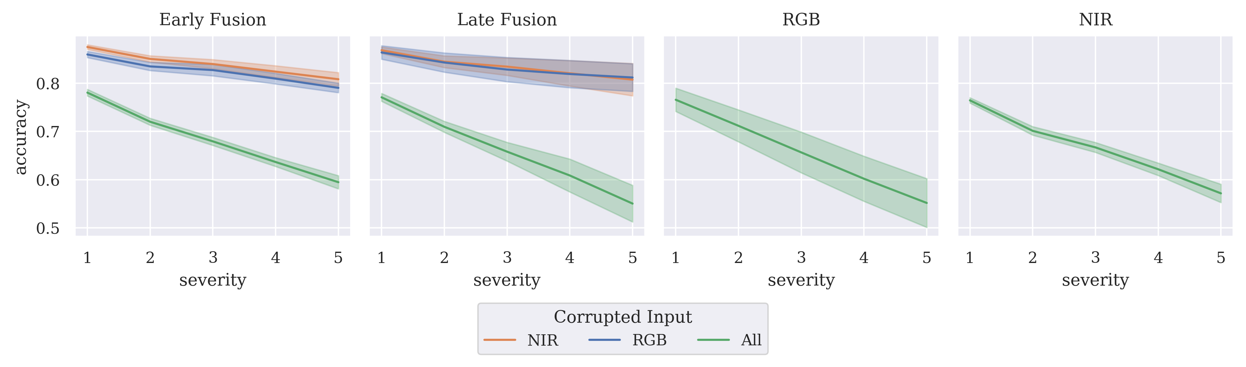
Figure 4: Corruption robustness of RarePlanes classifiers. Each subplot corresponds to a model architecture, and each line corresponds to a choice of input (RGB, NIR or both) to corrupt. Accuracy is averaged over all 15 types of corruptions, and confidence intervals are obtained from five evaluations of the experiment with independent random number generator seeds.

We evaluate each model on the corrupted images. Figure 4 shows how accuracy of RarePlanes classifiers degrades with increasing corruption severity. We can see that when all channels in an image are corrupted, there is a similar drop in performance for all of the models considered (i.e., all four channels input to an early fusion model or all three channels input to an RGB model). This suggests that none of the architectures considered provides a significant increase in overall robustness to natural corruptions.

For the early and late fusion models, we also test model performance when either RGB or NIR (but not both) inputs are corrupted. For the late fusion model, the effects of corrupting one (but not both) of {RGB, NIR} are more or less equal, while the early fusion model suffers a slightly greater drop in performance when RGB (but not NIR) channels are corrupted. We note that the confidence intervals in the early fusion model overlap; however, these results point in the same general direction as our perceptual score conclusions fig. 2: for early fusion models, RGB channels are weighted more heavily in predictions, and hence performance suffers more when RGB inputs are corrupted.

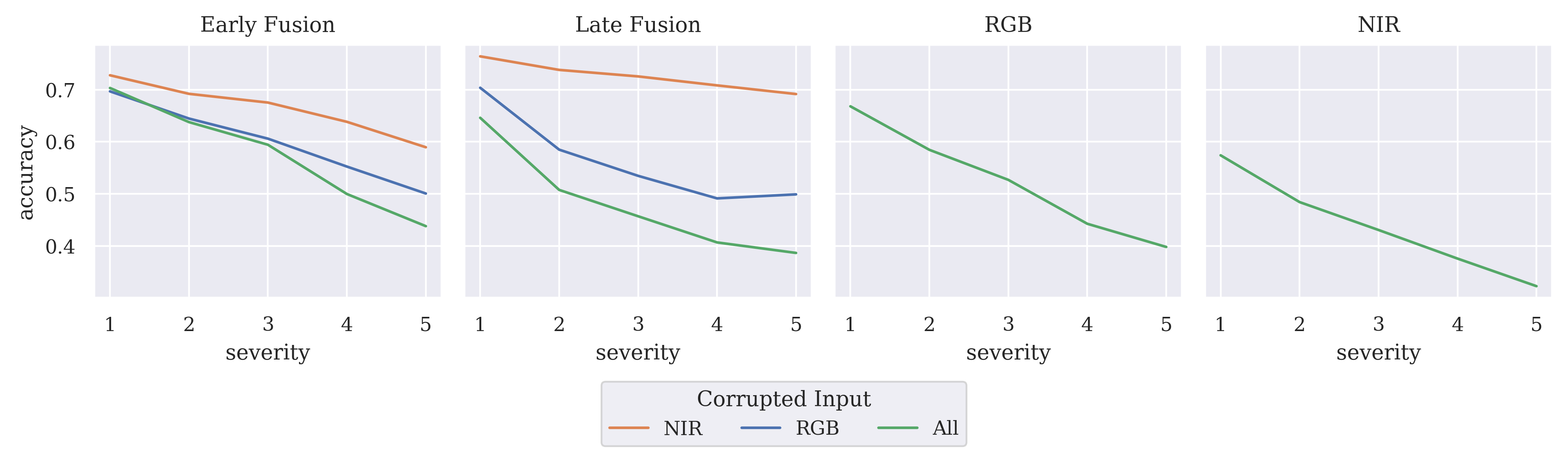
Figure 5: Corruption robustness of US3D segmentation models. Each subplot corresponds to a model architecture, and each line corresponds to a choice of input (RGB, NIR or both) to corrupt. IoU is averaged over all 15 types of corruptions.

Figure 5 shows how performance of US3D segmentation models (as measured by IoU) degrades with increasing corruption severity. When all input channels are corrupted (green line), the models show similar overall drops in performance, with the exception of the NIR-only model. The NIR-only model shows a larger drop in performance at all corruption severities, potentially suggesting that single-channel models are less robust to these kinds of natural corruptions. For both early and late fusion architectures, a greater performance drop is incurred when RGB (but not NIR) channels are corrupted. In fact, corrupting only RGB channels is almost as damaging as corrupting all inputs (both RGB+NIR). Notably in the case of late fusion, there is a large gap in robustness to corruptions of NIR inputs alone or RGB inputs alone. As was the case for the RarePlanes experiments, these corruption robustness results point in the same general direction as the perceptual score calculations in fig. 3. For example, the late fusion model had lower NIR perceptual scores than its early fusion counterpart (i.e., less reliant on NIR inputs), and it is more robust to NIR corruptions than the early fusion model.

We reiterate that due to computational costs we only train one US3D segmentation model of each architecture, but with this caveat it does appear that overall robustness in the case where all input channels are corrupted is decreasing from left to right in fig. 5. That is, the ranking of models according to corruption robustness is: early, late, rgb, nir. One potential explanation is that having more input channels (and hence more parameters) provides more robustness, although this would not explain why early fusion models seem to be more robust. Another possible explanation is that our models exhibit (positive) correlation between accuracy on clean test data and accuracy on corrupted data, as has been previously observed in the literature on robust RGB image classifiers [23]. Indeed, in fig. 10 we see that the ranking of our US3D segmentation models by test IoU is: early, late (tied), rgb, nir.

6 LIMITATIONS AND OPEN QUESTIONS

One limitation of our experiments is that the tasks considered are already tractable by a deep learning model using only RGB images; incorporating additional spectral bands offers at most incremental improvement. It would be interesting to carry out the evaluations of sections 4 and 5 for datasets and models that more obviously benefit from additional multispectral information beyond RGB. These might include ML models designed for tasks involving materials that can not be distinguished by RGB colors alone or environmental conditions in which NIR information is inherently valuable (such as pedestrian detection at night with RGB+NIR).

In this work we considered two basic forms of multispectral fusion (early and late), and although these arguably represent two interesting extremes there are many more sophisticated architectural designs for fusing multiple model inputs [24, 25, 24].

Evaluating robustness of image segmentation models to naturalistic corruptions is more complicated than in the case of classification tasks — In particular, there are some corruptions for which one might consider modifying segmentation labels in parallel with the underlying images (one example is the “elastic transform” corruption used in our experiments). In this work we did not apply any modifications to segmentation labels.

Finally, while we apply the same corruption algorithm to both the RGB and NIR channels, in some cases this is not physically realistic, for example snow is in fact dark in infrared channels. For a study of test-time robustness to more physically realistic corruptions of multispectral images, as well as robustness (or lack thereof) of multispectral deep learning models to adversarial corruptions of training data (i.e. data poisoning), we refer to [26].

7 CONCLUSION

This work evaluates the extent to which multispectral fusion neural networks with different underlying architectures

1. pay differing amounts of attention to different input spectral bands (RGB and NIR) as measured by the perceptual score metric and

2. exhibit varying levels of robustness to naturalistic corruptions affecting one or more input spectral bands.

We find that the answers to (i) and (ii) correlate as one might expect: paying more attention to RGB channels results in greater sensitivity to RGB corruptions. Interestingly, our experimental results for segmentation models on the US3D dataset contrast with those for classification models on the RarePlanes datsets: In the classification experiments, early fusion models had higher perceptual scores for RGB inputs, and late fusion models had slightly higher perceptual scores for NIR inputs, whereas both types of fusion segmentation models had higher perceptual scores for RGB inputs and the effect was more extreme for late fusion (results for corruption robustness follow this trend). This suggests that classification and segmentation models may make use of multispectral information in quite different ways.

Appendix A IMAGE PROCESSING

A.1 RarePlanes

The RarePlanes dataset includes both 8-bit RGB satellite imagery and 16-bit 8-band multispectral imagery, plus a panchromatic band. One of the goals of this work is to assess the utility of including additional channels as input to image segmentation models (e.g., near-infrared channels). In order to include channels beyond Red, Green, or Blue, we must work from the 16-bit 8-band images. We briefly describe our process for creating 8-bit, 8-band imagery, which consists of pansharpening, rescaling, contrast stretching, and gamma correcting the pixels in each channel independently. Specifically, the multispectral image is pansharpened to the panchromatic band resolution using a weighted Brovey algorithm [27]. The original 16-bit pixel values are rescaled to 8-bit, and a gamma correction is applied using $\gamma=2.2$ [28]. The bottom 1% of the pixel cumulative distribution function is clipped, and the pixels are rescaled such that the minimum and maximum pixel values are 0 and 255.

We note that when applied to the R, G, and B channels of the multispectral image products to generate 8-bit RGB images, this process produces images that are visually similar but not identical to the RGB images provided in Rare Planes. As such, the RGB model presented in this work cannot be perfectly compared to models published elsewhere trained on the RGB imagery included in RarePlanes. However, we felt that this approach provided the most fair comparison of model performance for different input channels, since the same processing was applied identically to each channel.

A.2 Urban Semantic 3D

US3D builds upon the SpaceNet Challenge 4 dataset (hereafter SN4) [29]. SN4 was originally designed for building footprint estimation in off-nadir imagery, and includes satellite imagery from Atlanta, GA for view angles between 7 an 50 degrees. US3D uses the subset of Atlanta, GA imagery from SN4 for which there exist matched LiDAR observations, and adds additional matched satellite imagery and LiDAR data in Jacksonville, FL and Omaha, NE. The Atlanta imagery is from Worldview-2, with ground sample distances (GSD) between 0.5m and 0.7m, and view angles between 7 and 40 degrees. The Jacksonville and Omaha imagery from Worldview-3, with GSD between 0.3m and 0.4m, and view angles between 5 and 30 degrees. As described below, we train and evaluate models using imagery from all three locations. We note however, that models trained solely on imagery from a single location will show variation in overall performance due to the variations in the scenery between locations (e.g., building density, seasonal changes in foliage and ground cover).

US3D includes both 8-bit RGB satellite imagery and 16-bit pansharpened 8-band multispectral imagery. Our process for creating 8-bit, 8-band imagery is similar to the process we used for RarePlanes, the main exception being that we omit pansharpening since it has already been applied to the multispectral images in US3D. The original 16-bit pixel values are rescaled to 8-bit, and a gamma correction is applied using $\gamma=2.2$. The bottom 1% of the pixel cumulative distribution function is clipped, and the pixels are rescaled such that the minimum and maximum pixel values in each channel are 0 and 255.

The US3D images are quite large (hundreds of thousands of pixels on a side) and must be broken up into smaller images in order to be processed by a segmentation deep learning model, a process sometimes called "tiling." Each of the large satellite images (and matched labels) was divided into 1024 pixel x 1024 pixel "tiles" without any overlap, producing 27,021 total images. All tiles from the same parent satellite image are kept together during the generation of training and validation splits to avoid cross contamination that could artificially inflate accuracies. An iterative approach was used to divide the satellite images into training, validation, and unseen hold-out (i.e., test) splits to ensure that the distributions of certain meta-data properties (location (Atlanta, Jacksonville, Omaha), view-angle, and azimuth angle) are relatively similar from one split to the next; in particular, this avoids the possibility that all images from a single location land in a single split. The final data splits included 21,776 tiles in training (70%), 2,102 tiles in validation (8%), and 3,142 tiles in the unseen, hold-out test split (12%). Models with near-infrared (NIR) input use the WorldView NIR2 channel, which covers 860-1040nm. The NIR2 band is sensitive to vegetation but is less affected by atmospheric absorption when compared with the NIR1 band. Segmentation labels are stored as 8-bit unsigned integers between 0 and 255 in TIF files; during training and evaluation we re-index these labels to integers between 0 and 6. We retain the "unclassified" labels during model training and evaluation, but do not include these classes in any metrics that average across all classes.

As in the case of RarePlanes, when this process is applied to the R, G, and B channels of the multispectral image products to generate 8-bit RGB images, it produces images that are visually similar but not identical to the RGB images provided in US3D. As such, the RGB model presented in this work cannot be perfectly compared to models published elsewhere trained on the RGB imagery included in US3D. Again, we felt that this approach provided the most fair comparison of model performance between different input channels, since the same processing technique is applied identically to each channel.

A.3 Applying Corruptions

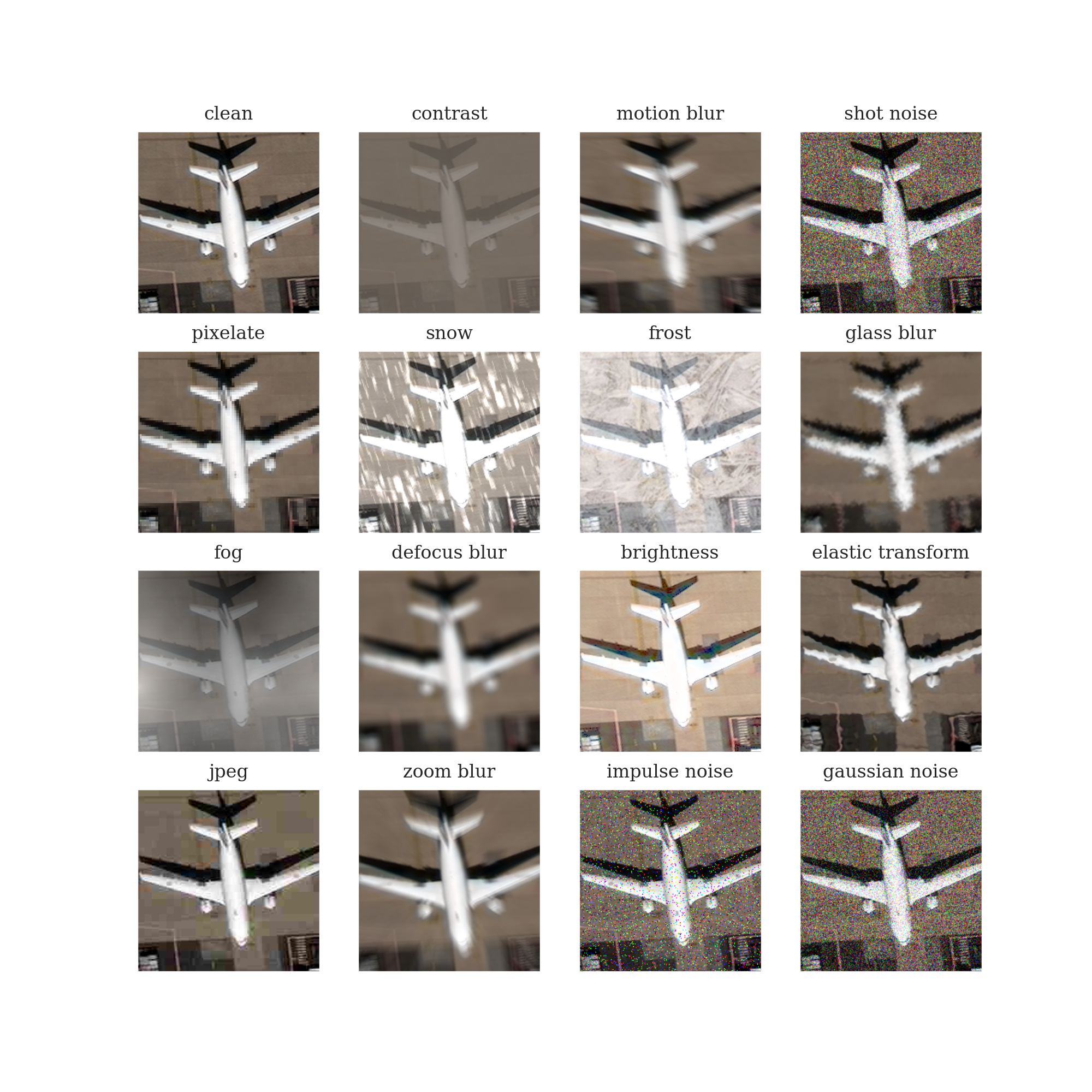
Figure 6: RGB corruptions of a RarePlane chip from our test set (severity level 3).

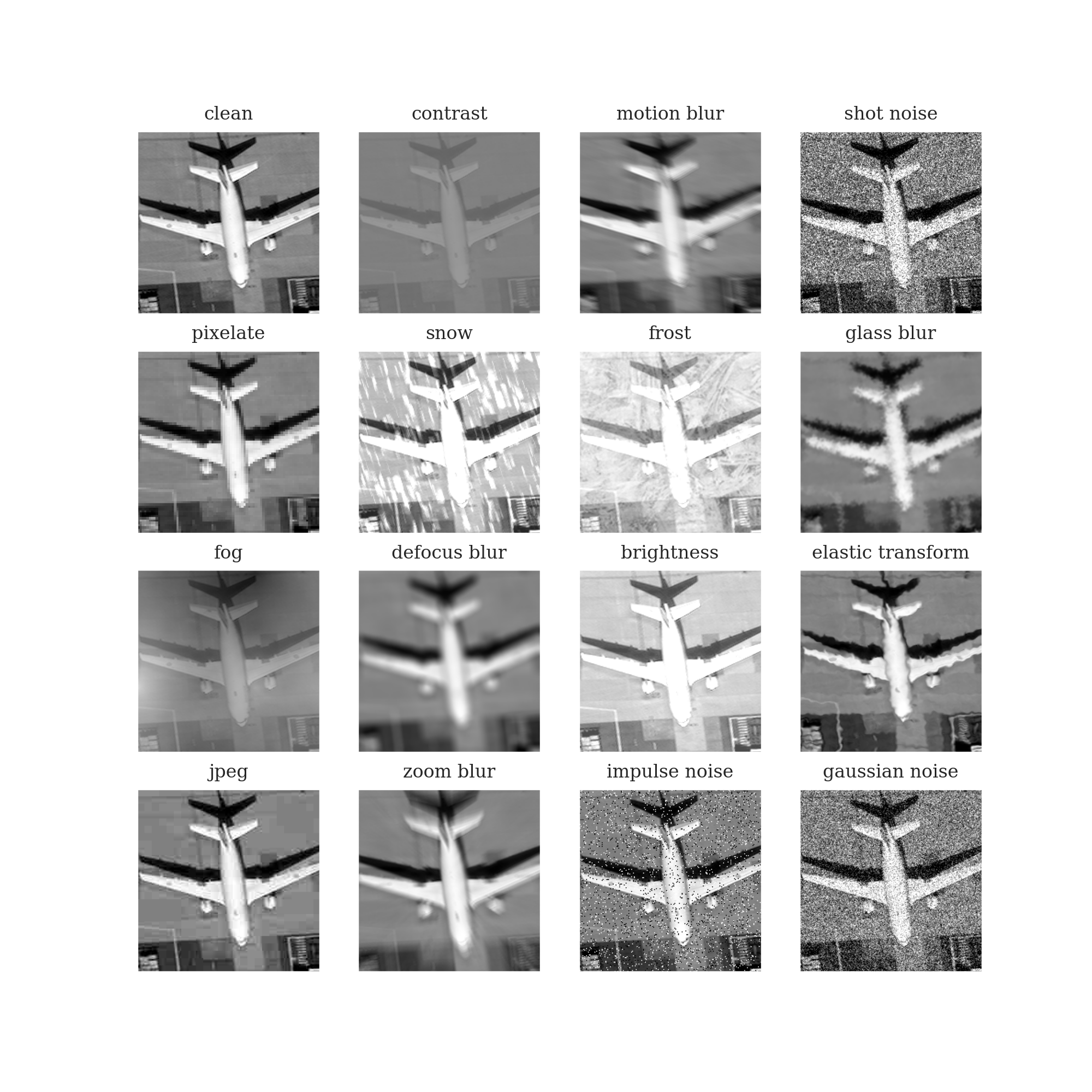
Figure 7: NIR corruptions of a RarePlane chip from our test set (severity level 3). Note that the motion blur (2nd row, 3rd column) is applied in the same direction as in fig. 6.

As mentioned above, we modify the code available at github.com/hendrycks/robustness (hereafter referred to as “the robustness library” or simply “robustness”), which was originally designed for $224\times 224$ RGB images, to achieve the following goals:

1. Arbitrary image resolution and aspect ratio (in fact this feature was already implemented in [30], though we did not discover that repository until after this work was completed). This was essential as the RarePlanes “chips” have varying resolution and aspect ratio, and while all US3D tiles are of shape $1024\times 1024$, that differs from the $224\times 224$ shape considered in robustness.

2. Input channels beyond RGB.

When applying corruptions to RGB+NIR images, we separate the 4-channel image into two 3-channel images, one containing the RGB channels and the other consisting of three stacked copies of the NIR channel. We then apply corruptions from robustness separately to each of these 3-channel images, with the following consideration: wherever physically sensible, we use the same randomness for both the RGB and NIR input. For example in the case of motion blur, we use the same velocity vector for both — not doing so would correspond to a physically unrealistic situation where the RGB and NIR sensors are moving in independent directions. On the other hand for corruptions such as shot noise modeling random processes affecting each pixel independently we use independent randomness for RGB and NIR. Corruptions of a RarePlanes test image can be seen in figs. 6 and 7.

We do not modify labels in any way. In the case of US3D one could argue that for some corruptions the segmentation labels should be modified. For example, “elastic transform” is implemented by applying localized permutations of some pixels and then blurring. Here it would make sense to apply at the exact same localized permutations to the per-pixel segmentation labels and then possibly blur them using soft labels (where each pixel is assigned to a probability distribution over segmentation classes). One could also imagine using soft label blurring for e.g. zoom or motion blur. Our reason for leaving segmentation labels fixed is pragmatic: in most cases we found where an argument could be made for modifying labels, doing so seemed to require working with $\text{num. classes}\times H\times W$ soft label tensors (possibly at an intermediate stage), and this would require modifications to multiple components of our pipeline, which (in keeping with standard practice) stores and utilizes labels as 8-bit RGB images with segmentation classes encoded as certain colors. Moreover, we emphasize that for most corruptions most severity levels the unmodified labels fairly reflect ground truth. With all of that said, in the case of elastic transform mentioned above we observed the bizarre experimental accuracy increasing as corruption severity increased — see fig. 8. Determining whether the results in that figure persist even after more care is taken with segmentation labels is a high priority item for future work.

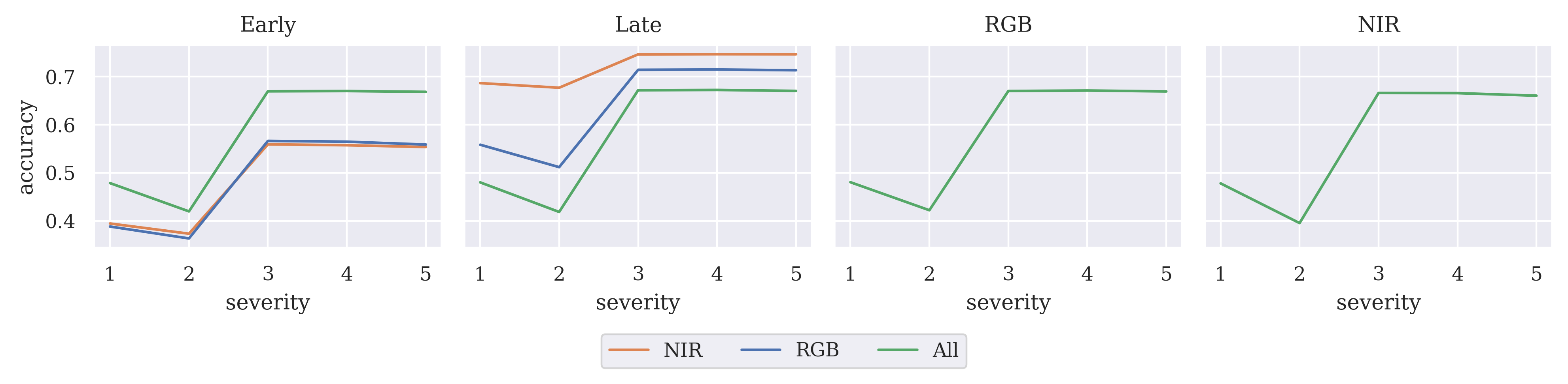
Figure 8: Results from the experiments summarized in fig. 5, restricting attention to the elastic transform corruption of [6].

Appendix B MODEL ARCHITECTURE AND TRAINING

For the RarePlanes experiments, all models are based on the ResNet34 architecture [15], pretrained on ImageNet (we use the weights from [31]).

For the early fusion model, we stack the RGB and NIR input channels to obtain a $4\times H\times W$ input tensor, and replace the ResNet34 first layer convolution weight, originally of shape $3\times C\times H\times W$, with a weight of shape $4\times C\times H\times W$ by repeating the red channel twice (i.e., we initialize the convolution weights applied to the NIR channel with those that were applied to the red channel in the ImageNet pretrained ResNet). For the pure NIR channel, we adopt a similar initialization strategy, but discarding the RGB weights since we only use one-channel NIR inputs (so in this case the first convolution weight has shape $1\times C\times H\times W$). For the pure RGB model of course no modifications are required.

In the late fusion model, we take a pure RGB and pure NIR architecture as described above, and remove their final fully connected layers: call these $f_{\text{rgb}}$ and $f_{\text{nir}}$. Given an input of the form $(x_{\text{rgb}},x_{\text{nir}})$, we use $f_{\text{rgb}}$ and $f_{\text{nir}}$ to compute two 512-dimensional feature vectors $f_{\text{rgb}}(x_{\text{rgb}})$ and $f_{\text{nir}}(x_{\text{nir}})$. These are then concatenated to obtain a 1024-dimensional feature vector $\mathrm{cat}(f_{\text{rgb}}(x_{\text{rgb}}),f_{\text{nir}}(x_{\text{nir}}))$. Finally, this is passed through a multi-layer perceptron with two 512-dimensional hidden layers.

For all training and evaluation, we “pixel normalize” input images, subtracting the a mean RGB+NIR four-dimensional vector, and dividing by a corresponding standard deviation. In the RarePlanes experiments we use the mean and standard deviation of the pretraining dataset (ImageNet) for RGB channels, and a mean and standard deviation computed from our RarePlanes images for the NIR channel. We fine tune on RarePlanes for 100 epochs using stochastic gradient descent with initial learning rate $10^{-3}$, weight decay $10^{-4}$ and momentum 0.9. We use distributed data parallel training with effective batch size 256 (128 $\times$ 2 GPUs). We use a “reduce-on-plateau” learning rate schedule that multiplies the learning rate by $0.1$ if training proceeds for 10 epochs without a $1\%$ increase in validation accuracy. We train five models of each fusion architecture with independent random seeds (randomness in play includes new model layers (all models include at least a new final classification layers) and SGD batching).

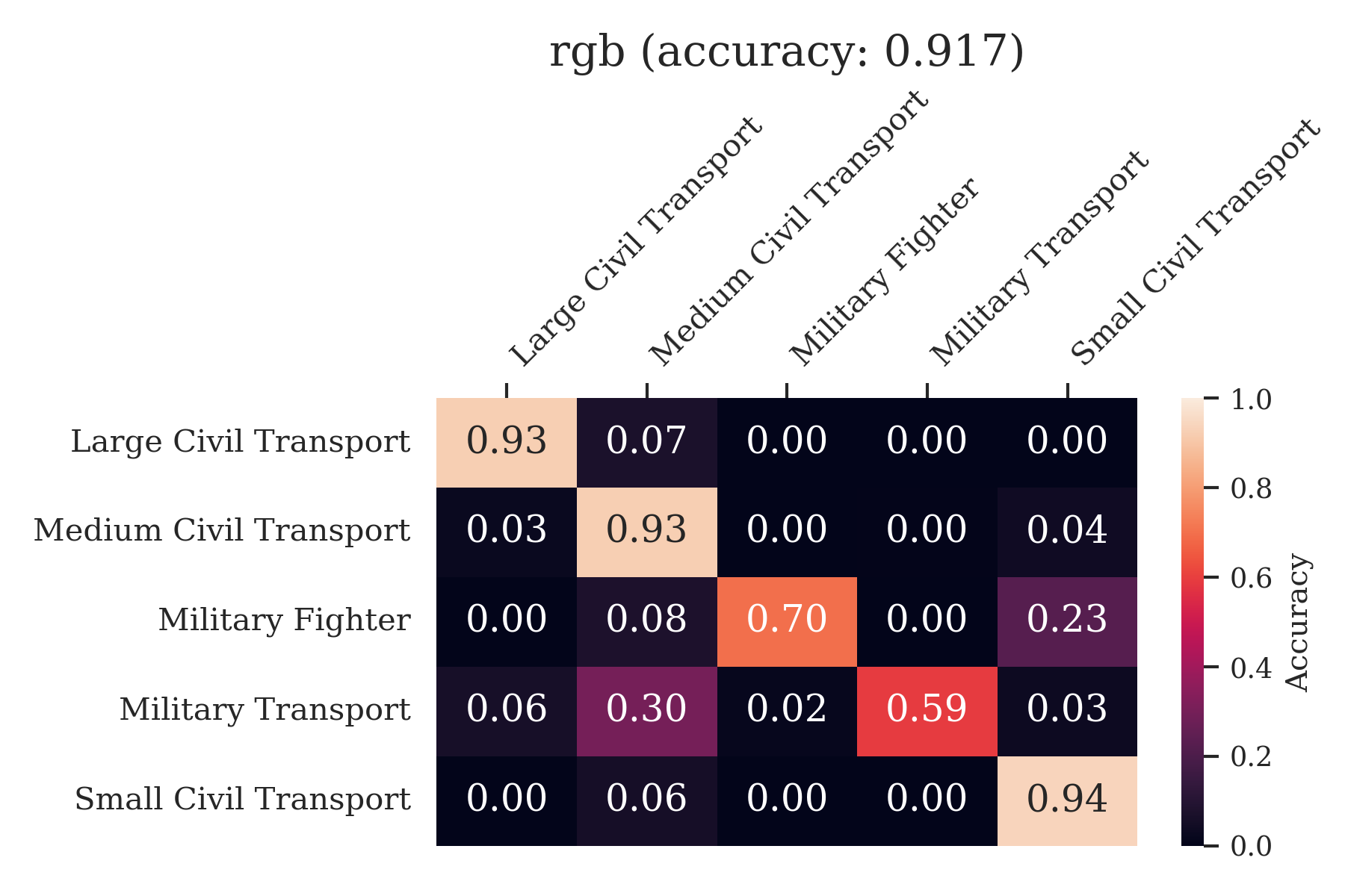
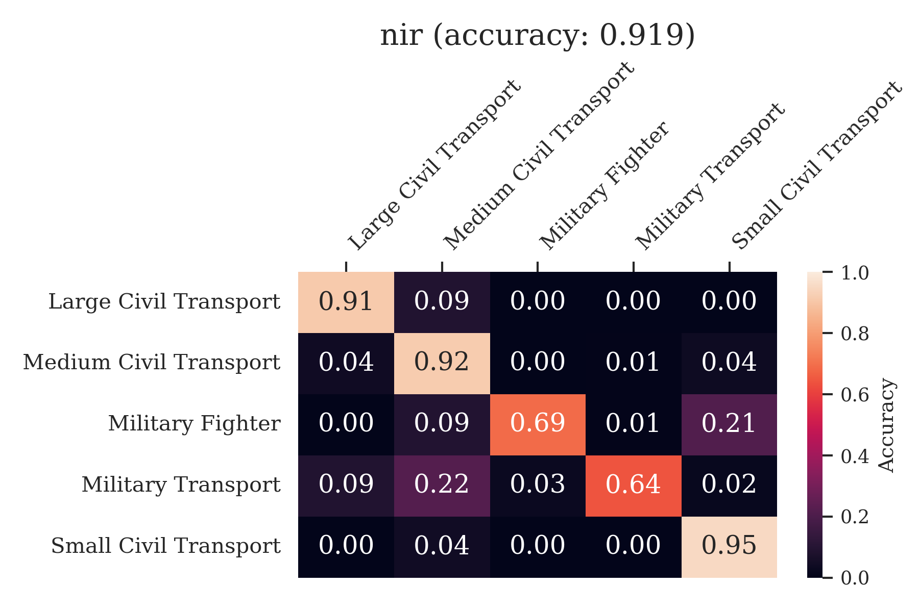
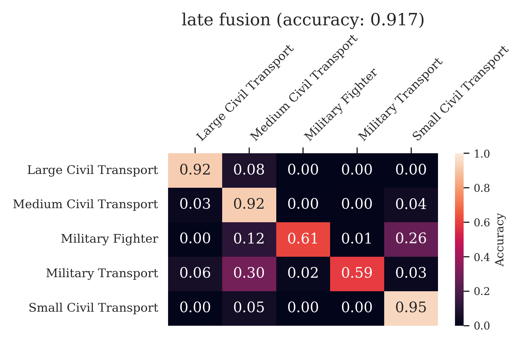
Figure 9: Test accuracies and confusion matrices for RGB+NIR RarePlanes models.

Figure 9 displays test accuracies and class confusion matrices of our trained RarePlanes classifiers. The accuracies of $\approx 92\%$ are respectable but by no means state-of-the-art.

All of our US3D segmentation models are based on DeepLabv3 with a ResNet50 backbone, pretrained on COCO [21] (again obtained from [31]). Our methods for defining RGB+NIR fusion architectures are similar to those described above for image classifiers, the difference being that we modify the ResNet50 backbone. In the case of early fusion and pure NIR models, we only need to modify the first layer convolution weights as described for the RarePlanes classifiers (and of course for the pure RGB model no modifications are necessary).

For the late fusion segmentation model, we start with pure RGB and pure NIR ResNet50 backbones: call these $f_{\text{rgb}}$ and $f_{\text{nir}}$. Given an input of the form $(x_{\text{rgb}},x_{\text{nir}})$, we use $f_{\text{rgb}}$ and $f_{\text{nir}}$ to compute two 2048-dimensional feature vectors $f_{\text{rgb}}(x_{\text{rgb}})$ and $f_{\text{nir}}(x_{\text{nir}})$. These are then concatenated to obtain a 4096-dimensional feature vector $\mathrm{cat}(f_{\text{rgb}}(x_{\text{rgb}}),f_{\text{nir}}(x_{\text{nir}}))$ which is then passed through the DeepLabv3 atrous convolution segmentation “head.”

In the US3D experiments we use the mean and standard deviation of ImageNet for RGB channels, and a mean and standard deviation of the ImageNet R channel for the NIR channel. We fine tune on US3D for 400 epochs using the Dice loss function optimized with Adam [32] with initial learning rate $5\times 10^{-4}$ and weight decay $10^{-5}$ (and PyTorch [33] defaults for all other Adam hyperparameters). We use distributed data parallel training with effective batch size 32 (4 $\times$ 8 GPUs). We use a “reduce-on-plateau” learning rate schedule that multiplies the learning rate by $0.5$ if training proceeds for 25 epochs without a relative $1\%$ increase in validation accuracy.

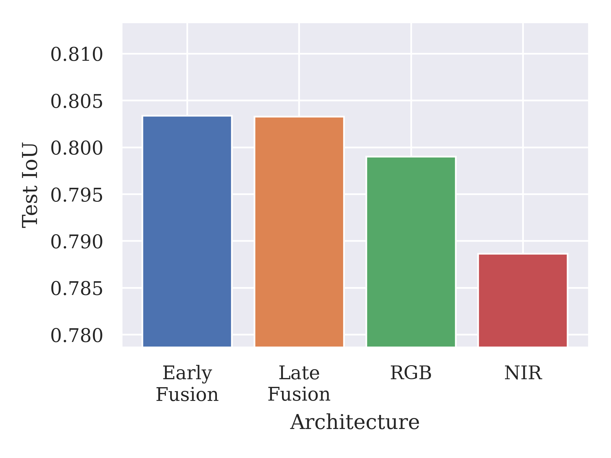
Figure 10: Intersection-over-Union (IoU) of US3D segmentation models.

Figure 10 displays test Intersection-over-Union (IoU) of our trained US3D segmentation models.

References

- [1] Gat, I., Schwartz, I., and Schwing, A., “Perceptual score: What data modalities does your model perceive?,” in [Advances in Neural Information Processing Systems ], Beygelzimer, A., Dauphin, Y., Liang, P., and Vaughan, J. W., eds. (2021).
- [2] Goyal, Y., Wu, Z., Ernst, J., Batra, D., Parikh, D., and Lee, S., “Counterfactual Visual Explanations,” in [Proceedings of the 36th International Conference on Machine Learning ], 2376–2384, PMLR (May 2019).
- [3] Chang, C.-H., Creager, E., Goldenberg, A., and Duvenaud, D., “Explaining Image Classifiers by Counterfactual Generation,” in [International Conference on Learning Representations ], (Feb. 2022).
- [4] Jain, S., Salman, H., Wong, E., Zhang, P., Vineet, V., Vemprala, S., and Madry, A., “Missingness Bias in Model Debugging,” (June 2022).
- [5] Hendrycks, D., Carlini, N., Schulman, J., and Steinhardt, J., “Unsolved Problems in ML Safety,” (June 2022).
- [6] Hendrycks, D. and Dietterich, T., “Benchmarking Neural Network Robustness to Common Corruptions and Perturbations,” (Mar. 2019).
- [7] Deng, J., Dong, W., Socher, R., Li, L.-J., Li, K., and Fei-Fei, L., “ImageNet: A large-scale hierarchical image database,” in [CVPR09 ], (2009).
- [8] Kamann, C. and Rother, C., “Benchmarking the Robustness of Semantic Segmentation Models,” 2020 IEEE/CVF Conference on Computer Vision and Pattern Recognition (CVPR) , 8825–8835 (June 2020).
- [9] Ortiz, A., Fuentes, O., Rosario, D., and Kiekintveld, C., “On the Defense Against Adversarial Examples Beyond the Visible Spectrum,” in [MILCOM 2018 - 2018 IEEE Military Communications Conference (MILCOM) ], 1–5 (Oct. 2018).
- [10] Yu, Y., Lee, H. J., Kim, B. C., Kim, J. U., and Ro, Y. M., “Investigating Vulnerability to Adversarial Examples on Multimodal Data Fusion in Deep Learning,” arXiv:2005.10987 [cs] (May 2020).
- [11] Du, A., Law, Y. W., Sasdelli, M., Chen, B., Clarke, K., Brown, M., and Chin, T.-J., “Adversarial Attacks against a Satellite-borne Multispectral Cloud Detector,” (Dec. 2021).
- [12] Gilmer, J., Adams, R. P., Goodfellow, I., Andersen, D., and Dahl, G. E., “Motivating the Rules of the Game for Adversarial Example Research,” (July 2018).
- [13] Podsiadlo, I., Paris, C., and Bruzzone, L., “A study of the robustness of the long short-term memory classifier to cloudy time series of multispectral images,” in [Image and Signal Processing for Remote Sensing XXVI ], 11533, 335–343, SPIE (Sept. 2020).
- [14] Shermeyer, J., Hossler, T., Etten, A. V., Hogan, D., Lewis, R., and Kim, D., “Rareplanes: Synthetic data takes flight,” 2021 IEEE Winter Conference on Applications of Computer Vision (WACV) , 207–217 (2020).
- [15] He, K., Zhang, X., Ren, S., and Sun, J., “Deep Residual Learning for Image Recognition,” arXiv:1512.03385 [cs] (Dec. 2015).
- [16] Christie, G., Munoz, R., Foster, K. H., Hagstrom, S. T., Hager, G. D., and Brown, M. Z., “Learning geocentric object pose in oblique monocular images,” in [CVPR ], (2020).
- [17] Christie, G., Foster, K. H., Hagstrom, S., Hager, G. D., and Brown, M. Z., “Single view geocentric pose in the wild,” in [CVPRW ], (2021).
- [18] Le Saux, B., Yokoya, N., Haensch, R., and Brown, M., “2019 ieee grss data fusion contest: Large-scale semantic 3d reconstruction [technical committees],” IEEE Geoscience and Remote Sensing Magazine 7(4), 33–36 (2019).
- [19] Bosch, M., Foster, K., Christie, G., Wang, S., Hager, G., and Brown, M., “Semantic stereo for incidental satellite images,” in [Proceedings - 2019 IEEE Winter Conference on Applications of Computer Vision, WACV 2019 ], Proceedings - 2019 IEEE Winter Conference on Applications of Computer Vision, WACV 2019, 1524–1532, Institute of Electrical and Electronics Engineers Inc. (Mar. 2019).
- [20] Chen, L.-C., Papandreou, G., Schroff, F., and Adam, H., “Rethinking Atrous Convolution for Semantic Image Segmentation,” (Dec. 2017).
- [21] Lin, T.-Y., Maire, M., Belongie, S., Hays, J., Perona, P., Ramanan, D., Dollár, P., and Zitnick, C. L., “Microsoft COCO: Common Objects in Context,” in [Computer Vision – ECCV 2014 ], Fleet, D., Pajdla, T., Schiele, B., and Tuytelaars, T., eds., Lecture Notes in Computer Science, 740–755, Springer International Publishing, Cham (2014).
- [22] Bubeck, S. and Sellke, M., “A universal law of robustness via isoperimetry,” in [Advances in Neural Information Processing Systems ], Ranzato, M., Beygelzimer, A., Dauphin, Y., Liang, P., and Vaughan, J. W., eds., 34, 28811–28822, Curran Associates, Inc. (2021).
- [23] Miller, J. P., Taori, R., Raghunathan, A., Sagawa, S., Koh, P. W., Shankar, V., Liang, P., Carmon, Y., and Schmidt, L., “Accuracy on the line: on the strong correlation between out-of-distribution and in-distribution generalization,” in [International Conference on Machine Learning ], 7721–7735, PMLR (2021).
- [24] Jayakumar, S. M., Menick, J., Czarnecki, W. M., Schwarz, J., Rae, J. W., Osindero, S., Teh, Y., Harley, T., and Pascanu, R., “Multiplicative Interactions and Where to Find Them,” in [ICLR ], (2020).
- [25] Baltrušaitis, T., Ahuja, C., and Morency, L.-P., “Multimodal Machine Learning: A Survey and Taxonomy,” IEEE Transactions on Pattern Analysis and Machine Intelligence (2019).
- [26] Bishoff, E., Godfrey, C., McKay, M., and Byler, E., “Quantifying the robustness of deep multispectral segmentation models against natural perturbations and data poisoning,” (May 2023).
- [27] Gillespie, A. R., Kahle, A. B., and Walker, R. E., “Color enhancement of highly correlated images. ii. channel ratio and “chromaticity” transformation techniques,” Remote Sensing of Environment 22(3), 343–365 (1987).
- [28] “Gamma correction,” Wikipedia (Feb. 2023).
- [29] Etten, A. V., Lindenbaum, D., and Bacastow, T. M., “Spacenet: A remote sensing dataset and challenge series,” CoRR abs/1807.01232 (2018).
- [30] Michaelis, C., Mitzkus, B., Geirhos, R., Rusak, E., Bringmann, O., Ecker, A. S., Bethge, M., and Brendel, W., “Benchmarking robustness in object detection: Autonomous driving when winter is coming,” arXiv preprint arXiv:1907.07484 (2019).
- [31] Marcel, S. and Rodriguez, Y., “Torchvision the machine-vision package of torch,” in [Proceedings of the 18th ACM International Conference on Multimedia ], MM ’10, 1485–1488, Association for Computing Machinery, New York, NY, USA (2010).
- [32] Kingma, D. P. and Ba, J., “Adam: A method for stochastic optimization,” in [3rd International Conference on Learning Representations, ICLR 2015, San Diego, CA, USA, May 7-9, 2015, Conference Track Proceedings ], Bengio, Y. and LeCun, Y., eds. (2015).
- [33] Paszke, A., Gross, S., Massa, F., Lerer, A., Bradbury, J., Chanan, G., Killeen, T., Lin, Z., Gimelshein, N., Antiga, L., Desmaison, A., Köpf, A., Yang, E., DeVito, Z., Raison, M., Tejani, A., Chilamkurthy, S., Steiner, B., Fang, L., Bai, J., and Chintala, S., [PyTorch: An Imperative Style, High-Performance Deep Learning Library ], Curran Associates Inc., Red Hook, NY, USA (2019).