Quantum Confusions, Cleared Up (or so I hope)

Abstract

I use an instrumental approach to investigate some commonly made claims about interpretations of quantum mechanics, especially those that pertain questions of locality. The here presented investigation builds on a recently proposed taxonomy for quantum mechanics interpretations [1].

1 Introduction

The major problem with quantum mechanics, it seems, is that we can’t agree what the problem is. Non-locality? Determinism? Realism? Incompleteness? The emergence of the classical world? All of those? None? For any possible position you could have on these points, you can find a scholar defending it. And how can we possibly solve a problem if we can’t agree on what the problem is in the first place?

Underlying this disagreement about what requires our attention is a conflation of terminology, a tower of Babel that has split our people into those who speak the language of Bohmian Mechanics, and those who understand only Many Worlds, settlements of natives who grew up with a disdain for philosophy and now correspond only in maths, immigrants who are fluent in causal models but can’t pronounce “phenomenology”, experimentalists who communicate solely with grunts and grins, and nomadic iconoclasts who have invented their own language. We fight over the meaning of words, not over physics. It’s what we’ve been doing for a century, it’s not getting us anywhere, and it’s about time we clean up our act.

In this paper, I want to look at some common confusions in the foundations of quantum mechanics using a purely instrumentalist approach. In particular, I want to address the questions whether the Collapse Postulate is necessary (it is, see Section 3), whether decoherence solves the measurement problem (partially, see Section 4), whether the Many Worlds Interpretation is Locally Causal (it is not, see Section 5), and whether Bohmian Mechanics solves the measurement problem (partially, see Section 6).

Throughout this paper, I use the convention $\hbar=1$.

2 Terminology

Before we start, we need to define some terms that will be used later on.

2.1 Instrumentalism

In this paper, I will take a purely instrumentalist approach. For me, quantum mechanics is a tool that we use to make predictions for our observations, no more, and no less. This does not imply that we only talk about what we can observe. Certainly an instrumentalist has their eyes on explaining observations, but if non-observable entities are useful to that end, of course the instrumentalist will happily employ them.

The instrumentalist approach will allow us to study the different interpretations and representations of quantum mechanics, using the taxonomy introduced in [1]. For this, we will need to carefully keep track of the assumptions that we make, of the input we require, and of the observations that we can predict.

The axioms of quantum mechanics can summarised as follows (see eg [2, 3]):

• The state of a system is described by a vector $|\Psi\rangle$ in a Hilbert space $\mathscr{H}$.

• Observables are described by Hermitian operators $\hat{O}$. Possible measurement outcomes correspond to one of the mutually orthogonal eigenvectors of the measurement observable $|O_{I}\rangle$.

• In the absence of a measurement, the time-evolution of the state is determined by the Schrödinger equation $i\partial_{t}|\Psi\rangle=\hat{H}|\Psi\rangle$.

• In the event of a measurement, the state of the system is updated to the eigenvector that corresponds to the measurement outcome $|\Psi\rangle\to|O_{I}\rangle$. This axiom is often called the “Collapse Postulate”.

• The probability of obtaining outcome $|O_{I}\rangle$ is given by $|\langle\Psi|O_{I}\rangle|^{2}$. This axiom is known as “Born’s Rule”.

• The state of a composite system is described by a vector $|\Psi\rangle$ in the tensor product of the Hilbert-spaces of the individual systems.

This list of axioms is not sufficient to make predictions. To do that, one also needs to at least define the Hamiltonian and the operator that corresponds to the variable that one wants to measure. However, we will in the following not need to talk about these, so we leave them aside here and just imagine that the system is sufficiently specified.

Once one has all those axioms in place, one inputs an initial state into the mathematical machinery of quantum mechanics. The output is then a final state, and from that—using Born’s Rule—a prediction for the probability of a particular measurement outcome. In the terms of [1], our list of axioms is a calculational model. For the rest of this paper, I will refer to this particular calculational model as the Copenhagen Model.

Following the terminology of [1], the Copenhagen Interpretation is then the set of all axiomatic formulations that are mathematically equivalent to the Copenhagen Model, and Standard Quantum Mechanics is further the set of all physically equivalent sets, that is, those who result in the same predictions for observables.

The Copenhagen Model is neither the best nor only approach to quantum mechanics. To begin with, its axioms could be rewritten into many other, mathematically equivalent, sets. A simple example might be that in the Heisenberg picture the state has no time evolution, but instead the operators do.

It is also quite possibly the case that there are axiomatic approaches to quantum mechanics which simplify the above axioms. This is because it has been pointed out previously (see eg [4] and [5]) that the probabilistic calculus we use in quantum mechanics is in some sense the simplest such calculus we could put onto a vector space. This is an interesting thought, but for our purposes it is not all that important. I here use the formulation with axioms A1 – A6 just because I believe it is one most readers will be familiar with, and it will be sufficient to make my points.

There are a few approaches to derive Born’s Rule from other assumptions, some more, some less convincing [6, 7, 4, 5, 8, 9, 10, 11]. While these are certainly worthwhile, we won’t need them here either. For our purposes we just need to note that there is no known derivation of Born’s Rule from the other 5 axioms on our list. To date, all known derivations require other assumptions in addition.

2.2 Local Causality

The Copenhagen Model—and because of that, the Copenhagen Interpretation—is not locally causal in Bell’s sense [12]. This is because making a measurement in one location—let’s call it $B$—can reveal information about what happens at another, space-like separated, region $A$, and that information was not contained on all hypersurfaces ($S$) in the backward lightcone of $A$ where they did not overlap with that of $B$. In mathematical terms, Local Causality requires $P(A|S,B)=P(A|S)~{}~{}\forall~{}~{}S$, where $P$ denotes probability (see Figure 1, after [12]).

The reason for this failure of Local Causality is that the wave-function does not contain sufficient information to calculate the measurement outcome at $A$, combined with the fact that the outcome at $B$ tells us something about the outcome at $A$. For an excellent summary of what Local Causality does and does not mean, see [13].

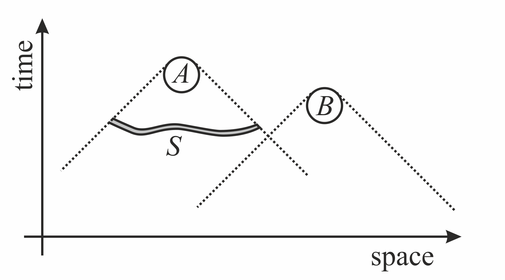
Figure 1: Local Causality means that given complete information on $S$, what happens at $B$ tells us nothing new about what happens at $A$. The Copenhagen Interpretation does not have this property.

The key reason quantum mechanics is non-local is therefore that the wave-function does not contain the entire information to predict the measurement outcome at $A$. The Collapse Postulate is a consequence of this: Once one has made a measurement at $B$, the information about the outcome must be included into the description of the system, otherwise the information is incomplete and the model is unable to correctly predict conditional probabilities.

Local Causality, defined in this way, is a property of a (mathematical) model, it is not a priori also a property of an (assumed to exist) underlying reality, and it is indeed perfectly suited for instrumentalists. Bell himself expressed this sentiment in [14]:

“I would insist here on the distinction between analyzing various physical theories, on the one hand, and philosophising about the unique real world on the other…I insist that [Bell’s theorem] is primarily an analysis of certain kinds of physical theory.”

Understanding that non-locality is a property of a model, we see that the non-locality of the Copenhagen Interpretation can be remedied by positing the existence of unknown information—usually called the “hidden variables”—that are added to $S$ (see Figure 1), propagate locally to $A$, and thereby make the information from the space-like separated measurement $B$ redundant for calculating the outcome of a measurement at $A$. This, in a nutshell, was the EPR argument [15], according to which the requirement of locality implies that quantum mechanics is incomplete.

We now know from Bell’s theorem [14] that any such model with hidden variables which returns us to Local Causality must violate Measurement Independence (aka non-contextuality), but that’s another story which has been told elsewhere [16, 17, 18].

2.3 Bell’s Theorem

Since Local Causality is a property of a model, observing violations of Bell’s inequality cannot tell us anything about nature itself, but merely about the properties of the model that we use to describe nature. As worthwhile as Bell’s theorem is, its implications are often overstated. For example in [19] we can read:

“Bell’s theorem actually shows that the observed probabilities in certain experiments (Einstein-Podolsky-Rosen-Bell experiments) are incompatible with locality, so our world must be non-local, and every theory in agreement with experiment must be non-local.”

The correct statement would have been: “Bell’s theorem shows that the observed probabilities in certain experiments are incompatible with the assumptions of Bell’s theorem. This means that any model which fulfils Local Causality and is in agreement with observation must violate Measurement Independence.”

I want to stress that this is not a matter of interpretation, it is merely a question of what can be concluded from observations and the mathematics that (correctly) describes these observations. A theorem about a certain class of models—those which fulfil the assumptions of the theorem, that is, Local Causality and Measurement Independence—can only tell us something about those models.

3 Is the Collapse Postulate Necessary?

It is sometimes questioned whether the Collapse Postulate is actually necessary (e.g. [2]). Especially defenders of the Many World’s Interpretation and its variants seem to think that the Collapse Postulate can be discarded. This question is a good starting point for our discussion because it makes clear why the instrumentalist approach is beneficial.

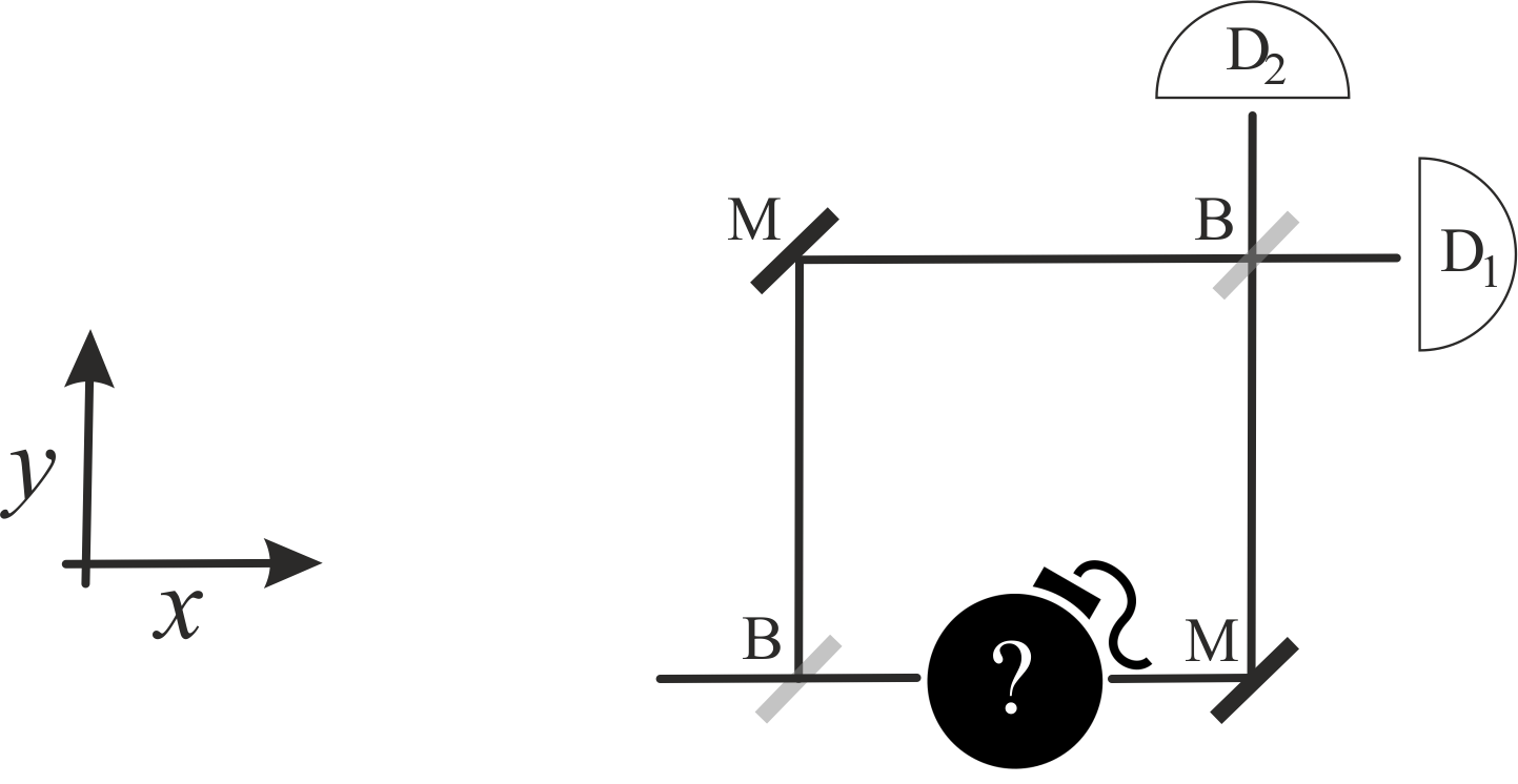
Figure 2: Sketch of the bomb experiment. Black bars marked M are mirrors, semi-transparent grey bars marked B are beam-splitters. Detector D₂ only registers a photon if the bomb was live and didn’t explode. The experiment can thus reveal information about a counterfactual event which didn’t happen.

Let us use as an example the Elitzur-Vaidman bomb detector [20] (Figure 2). In this experiment, one uses a single photon source and a Mach-Zehnder interferometer. The two paths are adjusted so that the signal always goes to detector D₁ by constructive interference, whereas the path to D₂ remains empty due to destructive interference. Then one places a “bomb” on one of the paths; in our example the lower path. If the bomb is live, it explodes if a photon hits it; if it’s a dud, it does nothing and the photon goes through undisturbed. While the bomb is certainly a memorable and illustrative example it really just plays the role of a detector that makes a which-path measurement. If the bomb is live, the detector is on; otherwise, it is off.

If the which-path detector is on (the bomb in live), there’s a 50% chance that it detects the photon (the bomb explodes). In the other 50% of cases, however, the photon goes to the second beam splitter and then has again a 50% chance (so 25% in total) to go to detector D₂.

The interesting thing about the bomb experiment (and similar setups like counterfactual computation [21]) is that the measurement outcomes on detectors D₁ and D₂ reveal something about a path that the photon did not take. This is because the only way that a photon can go to detector D₂ is to not take the lower path, and yet we learn from it that a live bomb was on that path.

Calculating the probabilities for the bomb experiment is straight forward using the Copenhagen Model. We will mark the wave-functions by the directions that they go, either $|x\rangle=(1,0)^{\rm T}$ for the horizontal direction or $|y\rangle=(0,1)^{\rm T}$ for the vertical one. The wave-function going in at the bottom right is $|\Psi\rangle_{\rm in}=|x\rangle$. The action of the beam splitters and mirrors is

$$B=B^{-1}=\frac{1}{\sqrt{2}}\left(\begin{array}[]{cc}1&1\\ 1&-1\end{array}\right)~{},~{}M=\left(\begin{array}[]{cc}0&1\\ 1&0\end{array}\right)~{}.$$ (5)

Without the bomb, the photon leaves the interferometer as $|\Psi\rangle_{\rm out}=BMB|\Psi\rangle_{\rm in}=|x\rangle$, so it goes into detector D₁ with probability 1, as expected.

If we place a detector on the lower arm and that does not detect the photon, we use the Collapse Postulate and update the wave-function to $|\Psi^{\prime}\rangle=|y\rangle$ before it hits the mirrors. The output of the interferometer is then $|\Psi\rangle_{\rm out}=BM|\Psi^{\prime}\rangle=(|x\rangle+|y\rangle)/\sqrt{2}$. We can then use Born’s Rule on this state to calculate the conditional probability for the case that the photon was not detected on the lower arm and correctly get a probability of $1/2$ in D₂ and D₁ likewise, or $1/4$ and $1/4$ for the total probabilities (the other $1/2$ being detected on the lower path). But without the Collapse Postulate, we have no instructions for what to do in case of a measurement. For all we can tell, the wave-function remains unchanged, but then Born’s Rule gives a wrong prediction.

Now you might argue that leaving the wave function unchanged when the photon is not detected on the lower path is not the proper way to to take into account the new information that we have obtained by making a measurement because Bayes’ Theorem should be applied here. And this is entirely correct, but how do you know that? Without the Collapse Postulate our axiomatic system does not contain such an instruction.

Again, please put yourself in the shoes of an instrumentalist. The instrumentalist just wants to know what to calculate. He or she does not know what you think the wave-function means. Therefore, if not the Collapse Postulate itself, the instrumentalist needs another instruction to account for the change in case of a measurement.

I believe the reason this fact sometimes becomes muddied up is that the Collapse Postulate describes exactly how one would expect conditional probabilities in a statistical ensemble to behave, so it seems obviously true. Indeed, it would be, if we were dealing with a statistical ensemble. If we had a statistical ensemble, then we could derive conditional probabilities from it. But we are dealing with one wave-function of one single photon. And whether or not it seems obvious to you, given what you know about probabilities and quantum mechanics, one still has to take this update rule into account in the formulation of the theory, somehow. This is exactly what the Collapse Postulate does, and this is exactly why quantum mechanics is not locally causal.

You could argue that maybe “Collapse Postulate” is not a particularly good name (and I would agree), but you will still need this—or an equivalent—assumption in the axioms to obtain the correct conditional probabilities. The axioms need to somehow contain the information that the wave-function updates as if we were dealing with a statistical ensemble. (One way to do this is just by stating that this is how it updates, which is how the Statistical Interpretation works [3].)

For the instrumentalist, the maths is clear: One cannot simply discard the Collapse Postulate from the Copenhagen Model and make do with the remaining 5 axioms. It just does not work. If one removes the Collapse Postulate, at least it needs to be replaced with something else, otherwise there are cases for which the model is unable to give correct predictions.

4 Does Decoherence Solve the Measurement Problem?

Let us move on to a related question, that is whether decoherence solves the measurement problem.

The measurement problem has many aspects [22, 23, 24]. We will here focus on two of them. First, there’s the question what a measurement is (beyond the ”we know it when we see it” take) and second, whether we can get rid of the non-locality of the measurement process.

Decoherence is often described as the result of interactions with an environment that lead to a loss of quantum properties, mathematically captured by the transition from a pure to a mixed state. For example, according to Zurek “Environment can destroy coherence between the states of a quantum system. This is decoherence.” [25] (emph original). But interactions with the environment—as all interactions in quantum mechanics—are unitary transformations. They cannot transform pure to mixed states.

Since interactions alone cannot bring about mixed states, in decoherence approaches one follows up on the increase of entanglement by the operation of mathematically “tracing out” (basically: summing over) that part of the system which was designated as the environment. Tracing out is usually not interpreted as a physical process but as reflecting the experimentalist’s lack of knowledge. Again, however, we take an instrumentalist approach and do not care about interpretations. We simply note that if we want to use traces to calculate probabilities, then we need to add this procedure to the axioms. And then we will need further assumptions about just what to trace out.

If one adds these assumptions, this will indeed produce a mixed state. But in the Copenhagen Model, the outcome of a measurement is not a mixed state. It is another pure state, one that is an eigenstate of the measurement variable. Decoherence therefore does not replace the Collapse Postulate. Consequently, it cannot restore Local Causality.

Let us draw again on our earlier example of the bomb experiment to see that. After the photon goes through the first beam-splitter its wave-function is $|\Psi\rangle=(|x\rangle+|y\rangle)/\sqrt{2}$. The corresponding density matrix is

$$\hat{\rho}=|\Psi\rangle\langle\Psi|=\frac{1}{2}\left(\begin{array}[]{cc}1&1\\ 1&1\end{array}\right)~{}.$$ (8)

Decoherence with a suitably defined entanglement followed by tracing out the environment effectively removes the off-diagonal entries of the density matrix. So, after the which-path measurement we have

$$\hat{\rho}^{\prime}=\frac{1}{2}\left(\begin{array}[]{cc}1&0\\ 0&1\end{array}\right)~{},$$ (11)

which describes a state that is no longer in a superposition, but instead in either upper or lower path with probability $1/2$. This density matrix, importantly, no longer corresponds to a wave-function. But what are we to do with it now?

We can apply the actions of mirrors and beam splitters and calculate $\hat{\rho}^{\prime\prime}=BMB\hat{\rho}^{\prime}BMB$, but this would give us probability $1/2$ for each of the detectors (rather than $1/4$, which would be correct). ”Yes, but,” I image you objecting exasperated, ”Of course we need to take into account that we are now only looking at the case in which the photon was not detected on the lower path! We need to update the probabilities accordingly!” And this is entirely correct—if you already know how quantum mechanics works. But without the Collapse Postulate, there is no such instruction in the axioms, hence the instrumentalist does not know what to do.

The problem is, decoherence in and of itself keeps all possible measurement outcomes, indefinitely, and that just gives incorrect probabilities once we observed a particular outcome. A photon that was not detected on the lower path has probability zero to be on the lower path. This needs to reflect somehow in the description of the system. Throwing out the Collapse Postulate makes this impossible. Consequently, even with decoherence we still need the Collapse Postulate, in the sense that once we know the photon is not on the lower path, we need update the density matrix (or at least readjust the final probabilities to conditional ones). Either way you do it, this update is exactly as non-local as the Collapse Postulate itself.

This should not be surprising because we already saw earlier that non-locality of the Copenhagen Model has nothing to do with the Collapse Postulate per se. It is rather the lack of information in the wave-function together with the fact that an observation in one location can tell us something about the measurement outcome in another location. Describing this observation is what requires some non-local update, regardless of how one wants to express it mathematically. The only thing we can do is to prevent this non-locality from being a fundamental property of reality (rather than just a property of a model which describes knowledge) by introducing hidden variables which can locally transport the information.

Another way to see that decoherence cannot possibly restore locality is to note that if the interactions that create entanglement are to be local, then they can start at the earliest when the prepared state reaches the detector. At that point, however, it is simply too late for the wave-function to locally go into an eigenstate. (One can imagine cases where decoherence starts earlier because particles do not propagate through vacuum, but this generically does not work.)

We have seen that decoherence cannot restore Local Causality, but does it explain in which cases a measurement takes place? One could argue that decoherence at least tells us when the measurement process is completed, and what the variable is that one measures. Alas, this is not the case because decoherence requires one to specify what the “environment” is. We need to know what to trace out to get the mixed state to begin with. Indeed, the notion of entanglement itself makes no sense unless we divide up the system into at least two partitions. That decoherence does not resolve this aspect of the measurement problem has been discussed previously in more detail in [26, 27].

To put this problem in somewhat simpler terms, suppose that I give you a wave-function that I tell you contains a prepared state and all the particles of the detector and their environment, but I don’t tell you which part is which. To solve the measurement problem you would have to know whether this combined system is going to perform a measurement and if so, of which variable. Saying “decoherence” does not suffice to answer this question.

There have been many attempts to try and find a definition that would break up a generic state into the prepared state (that one wants to measure), the environment, and the pointer states of the detector. If one knew how to do that, then one would know what to trace out, and decoherence could be used to identify the measurement variable and the circumstances under which to apply the Collapse Postulate. I would say that as to date none of these approaches have been entirely convincing, and somewhat vaguely conclude that while decoherence has the potential to solve this aspect of the measurement problem, it hasn’t yet been satisfactorily done.

This is not to belittle the achievements of the decoherence program. Studying decoherence has been extremely useful in experimental settings, e.g. to understand the effects of the environment [28].

Some physicists have tried to “solve” the measurement problem by simply redefining the Collapse Postulate to mean that a measurement results in a mixed density operator. A prominent example of this confusion can be found in [29]. Needless to say, taking something else and naming it “Collapse Postulate” does not solve any problems.

5 Is the Many Worlds Interpretation Local?

Understanding the shortcomings of the decoherence approach also useful to putting the Many Worlds Interpretation into perspective, which we will turn to now.

5.1 Many Worlds Recap

There are many Many Worlds Interpretations [30, 31, 32, 33, 34, 35, 36, 37, 38, 39], but they have one thing in common: The idea that it is possible to remove the Collapse Postulate from the axioms of quantum mechanics. In the Many Worlds approach one posits that all possible outcomes of an experiment happen, each in its own universe, it’s just that we only ever experience one possible outcome. The process in which the other possible outcomes become inaccessible to us is referred to as the “branching” or “splitting” of worlds.

We put on our instrumentalist hat and remember that we cannot simply throw out the Collapse Postulate if we want to get correct predictions for conditional probabilities, and that decoherence does not solve the problem because it is missing an update rule. Consequently, if one does calculations in any Many Worlds approach, one must effectively replace the Collapse Postulate by other assumptions, notably about what happens to observers and/or measurement devices when worlds branch. Suitably done, the outcome for the measurement probabilities is then the same as in the Copenhagen Model.

Unfortunately, the new assumptions which must be added to make the Many Worlds Interpretation work are often not explicitly stated but implicitly appear in elaborations on what an observer is. To make a long story short, the relevant property of an observer in a Many Worlds Interpretation is that they can still can only see one outcome of an experiment. This property cannot be derived from axioms A1 – A5. If it was only for those assumptions then any object (including observers) would deterministically split into superpositions with any experiment for which the forward evolution of the initial state is not an eigenstate of the measurement operator. The Many Worlds Interpretation therefore must sneak back in the Collapse Postulate somehow. Usually this is done by implicitly assuming that an observer is not something that exists in multiple branches at the same time.

A typical example of how this happens can be found in [38] where we can read:

“Because these environment states are and will be orthogonal […] each component evolving in accordance with the Schrödinger equation as if the other were not present. They can thus be treated as separate worlds (or collections of worlds) since they are effectively causally isolated and within each of them there are versions of Alice having clear and determinate experiences.”

In this paragraph, the authors of the paper use decoherence (that, as usual, draws on a pre-defined environment) to motivate a statement about mathematically ill-defined terms like “Alice” and her “experience”. It remains unexplained why the time-evolution of an object once called Alice is later no longer just Alice but multiple versions of something also called Alice. (According to the authors, “This is a tricky metaphysical question upon which we will not speculate.”) The rest of the paper is then dedicated to developing a rule to update probabilities in the Many Worlds Interpretation, so that they agree with the Collapse Postulate of the Copenhagen Model. Well done.

I would like to make clear that I have no issue with the way that Carroll et al interpret what is effectively the Collapse Postulate. My point is merely that it does not mathematically follow from the Schrödinger equation and the other 4 axioms, excluding the Collapse Postulate. If the Collapse Postulate would mathematically follow from the other 5 axioms of the Copenhagen Model, then it would do so regardless of how one interprets the mathematics. It does not. Hence, if we want a mathematical procedure with the same result as the Collapse Postulate, that will require new assumptions. If one does not make those extra assumptions, one has a theory that does not make correct predictions.

Once one equips the Many Worlds Interpretation with suitable assumptions to reproduce the Collapse Postulate, it makes the same predictions as the Copenhagen Model. Because of the extra assumptions about observers, it is however not mathematically equivalent. In the terms of [1], therefore, it is not a representation of the Copenhagen Model, but a physically equivalent interpretation, and can be understood as standard quantum mechanics.

The Many Worlds Interpretation is temporally deterministic, again using the terms of [1]. This means that the final state can be predicted with certainty from the initial state. Determinism is reestablished by positing that all possible outcomes of an experiment happen, we just only see one, whose outcome we can then not predict. The Many Worlds Interpretation is therefore not predictive, again in the terms of [1]. We note that this has nothing to do with quantum theory in particular—any non-deterministic theory could be converted to a deterministic yet non-predictive theory in this way, it is just that the need usually does not arise.

5.2 Locality in the Many Worlds Interpretation

It follows from the above that the Many Worlds Interpretation is exactly as non-local as the Copenhagen Model. This can be seen as follows.

Remember that the reason the Copenhagen Model is non-local is that a measurement in one location can reveal information about a measurement in another, space-like separated region, and that this information could not be obtained from the wave-function.

Well, the only information we have in the Many Worlds Interpretation is also that in the wave-function, and for what our observations are concerned, it give the same predictions as the Copenhagen Model. Hence, it is also non-local. You can believe in as many other universes as you wish, making a measurement on one end of the wave-function will de facto reveal something about the outcome on the other end. If you know a particle was measured in one place, you know it wasn’t measured in another place. This, combined with the impossibility of predicting the measurement outcome from the wave-function alone, makes the Copenhagen Model non-local, and the Many Worlds Interpretation changes nothing about that.

I believe the reason that Many World supporters are confused about this point is the following. If you think that the origin of non-locality in the Copenhagen Model is the Collapse Postulate, and you discard of the Collapse Postulate, then what’s left should be local.

However, the non-locality of the Copenhagen Model does not come from the Collapse Postulate per se, it comes from the lack of information about measurement outcomes in the wave-function, combined with the fact that making a measurement in one place reveals something about another place. And the Many Worlds Interpretation doesn’t change either. It does not help that, as pointed out in [40, 41], the word “locality” in the context of Many Worlds Interpretations has been used with different meanings.

Neither does it help to add more complicated stories about how the branching occurs. The local branching idea (of which, again, there are several variants [42, 10, 43]) has it that the splitting of the worlds obeys the speed-of-light limit. For this reason, a measurement in $B$ in Figure 1 does not split the world in $A$ instantaneously. It is only when the two come into causal contact and observers from both places can compare their measurements that the split must have been completed.

But for us instrumentalist this story is irrelevant. We take the measurement results from $A$ and $B$ and apply our definition of Local Causality. It is violated, and that’s that. Whether you think there were multiple different universes with different outcomes at $A$ before we compared both records is irrelevant for the fact that the records which we do have in our universe show these correlations. And since there is not enough information in the wave-function to predict $A$ without the information from $B$, Local Causality is violated. Stories about local branchings do not matter. (Unless the branching contains additional information about the measurements that will be made, in which case Local Causality can be restored by violating Measurement Independence instead.)

If one makes the mistake of thinking that the Many Worlds Interpretation is locally causal, then one has another problem, which is Bell’s theorem. According to Bell’s theorem, a theory can only be locally causal if it introduces hidden variables which violate Measurement Independence. The Many Worlds Interpretation does not do that, so what gives?

Hence emerged the idea of an additional assumption in Bell’s theorem which is that measurements have only one definite outcome. It is sometimes called the “one world” [39] assumption,“single world” assumption [44], or the “definite outcome” assumption [40]. This peculiar idea has it that the Many Worlds Interpretation evades the conclusion of Bell’s theorem by allowing more than one measurement outcome, each in a separate universe.

But all that throwing out the assumption of a definite outcome does is render Bell’s theorem useless. Bell’s theorem is a statement about correlations that we observe. It is a fact, not merely a mathematical assumption, that we observe only one outcome of an experiment. If one removes this assumption, then one is left with a theorem about something that does not describe our observations.

My experience with Many Worlds enthusiasts is that they follow a motte-and-bailey approach. For those not familiar with this logical fallacy, it consists of first building up an easy to defend argument (the motte) and then using mutual agreement on that easy argument to claim victory on a different argument (the bailey). It’s an example of what is also known as the bait-and-switch tactic.

The argument of Many Worlds defenders goes like this. First, they will claim that discarding of the Collapse Postulate creates a model which is axiomatically simpler than the Copenhagen Model. Dropping this postulate moreover removes the non-local element of the dynamical law. And this is both correct, but fails to mention that removing the Collapse Postulate leaves one with a model that may be simple and local, but generically gives wrong predictions.

Then happens the switch, in which the Many Worlds fan needs to add new assumptions to make the same predictions as the Copenhagen Model does. It is highly questionable that the total of their new assumptions is any simpler than the Collapse Postulate, but this is not an argument I want to make here. However, any set of assumptions that leads to the same observational outcome as the Collapse Postulate without also equipping the wave-function with more information about the measurement outcome, will inevitably be exactly as non-local as the Copenhagen Model.

The trick of Many Worlds defenders is now to first get you to agree to take their bait argument—a model which may be simple and local but does not make correct predictions—and then claim you agreed to their elaborations on different versions of Alice.

All of this is not to say that there is something wrong with the Many Worlds Interpretation (in the bailey-version equipped with sufficient assumptions to produce correct predictions). As an interpretation of quantum mechanics it is not necessarily any worse than the Copenhagen Model. Though personally I think using the Collapse Postulate is simpler than bothering with splitting worlds and such. I would recommend to anyone who thinks that the Many Worlds Interpretation is simpler than using the Collapse Postulate that they read this paper [38], track all assumptions, and decide for themselves.

It is indeed possible to formulate some variants of Many Worlds models that are local, but these violate Measurement Independence. This should not be surprising because this follows from Bell’s theorem. For a discussion of examples, see [40]. Note that in the example for a local version of Many Worlds in the last section of [40], the branching depends on the measurement settings, and hence violates Measurement Independence—as one expects.

6 Does Bohmian Mechanics Solve the Measurement Problem?

6.1 Bohmian Mechanics Recap

Bohmian Mechanics [45, 46] uses the Schrödinger equation (A3) for the wave-function $\psi$ in configuration space

$${\rm i}\frac{\partial\psi(\boldsymbol{q},t)}{\partial t}=-\sum_{k=1}^{N}\frac{1}{2m_{k}}\Delta_{k}\psi(\boldsymbol{q},t)+V(\boldsymbol{q},t)\psi(\boldsymbol{q},t)~{},$$ (12)

where ${\boldsymbol{q}}=(q_{1},q_{2}\dots q_{N})$ are spatial coordinates, $V$ is a potential, and $m_{k}$ are the particle masses. So far, this looks like ordinary quantum mechanics. But then one posits that the state of a system is described by $N$ particles whose actual position is described by $\boldsymbol{Q}=\{Q_{1}(t),Q_{2}(t)\dots Q_{N}(t)\}$. The particles are assumed to have velocities given by

$$m_{k}\frac{dQ_{i}}{dt}={\rm Im}\frac{\psi*\nabla_{k}\psi}{\psi^{*}\psi}(\boldsymbol{Q}(t),t)~{}.$$ (13)

In Bohmian Mechanics, one reformulates Born’s Rule (A5) into the “quantum equilibrium hypothesis”, according to which the probability distribution of the particles described by $\boldsymbol{Q}$ is of the form $|\psi(\boldsymbol{q},t)|^{2}$. One can then show that if this equilibrium hypothesis is fulfilled at one time, it will be fulfilled at all times. One hence only needs it as an assumption about the initial state. One further assumes that the state of the system is really one particular value of $\boldsymbol{Q}$, though one does not know which. $\boldsymbol{Q}$ serves the role of the hidden variables.

The picture that Bohmian Mechanics offers is that the wave-function of the Copenhagen Model serves as a guiding field for point-like particles. The indeterminism of quantum mechanics arises from our lack of knowledge about the exact initial state of the Bohmian particle (or particles, if there are several).

Bohmian Mechanics then does not need the Collapse Postulate. This is because introducing the new variables $Q_{i}$ and positing that the state is only in one of the possible configurations, means that a measurement merely reveals which state the system was really in. The pilot wave itself is not updated upon measurement. This gives rise to what has been dubbed “empty waves” [47, 48, 49]. These are valleys in the pilot wave where a particle might have gone but did not, and which seemingly continue forever.

Bohmian Mechanics also does not use axiom A2. Instead, one assumes that the only variable one can measure is the position of the Bohmian particles. Any other measurement variable that one might use in quantum mechanics must be converted into a position measurement (see e.g. [50]). This is an extremely important assumption of Bohmian Mechanics, because it means that all details of the measurement settings—which play a key role in Bell’s notion of Local Causality—must be encoded as transformations of the state that occur before the actual measurement. The measurement settings hence become part of the Hamiltonian evolution.

This axiomatic form of Bohmian Mechanics is not mathematically equivalent to the Copenhagen Model. One way to see this is to note that there is no equivalent to the particle positions $Q_{k}(t)$ in the Copenhagen Model. An easier way to see it is that if the two were equivalent, then the pilot wave should not have empty branches. However, Bohmian Mechanics in its original form is generally believed to make the same predictions as the Copenhagen Model, at least for a non-relativistic Hamiltonian (see e.g. [51]). In the terms of [1] then, Bohmian Mechanics is an interpretation of the Copenhagen Model, but not a representation.

Bohmian Mechanics is also a temporally deterministic model, using the terminology of [1]. The theory is, however, not predictable because while the initial state predicts the final state, one also cannot know the initial state exactly, hence not predict the final state. This trade-off can be done for any non-deterministic theory: By introducing hidden variables that are unmeasurable out of principle, the temporally non-deterministic time-evolution can be converted into a deterministic, yet unpredictable one.

There are today many slightly different formulations of Bohmian Mechanics [52, 53, 54, 55, 56, 57, 58, 59, 60, 61, 62, 63], and it is beyond the scope of this paper to go through all of them, but I believe they are mostly interpretations of the Copenhagen Model. An exception are those variants which do not use quantum equilibrium as one of their assumptions [64, 65]. Since they give under certain circumstances different predictions from the Copenhagen Model, they are modifications instead of interpretations (again using the terminology of [1]). Those modifications will not be considered below.

6.2 Contextuality in Bohmian Mechanics

It is generally acknowledged that Bohmian Mechanics is not local because the particle velocities at one location depend on the particle positions on all other locations. This is apparent from Eq. (13), because it implies that the dynamical evolution of the $k$-th particle depends on the position of all other particles—regardless of how far away they might be. If we apply Bell’s criterion of Local Causality, $P(A|S,B)=P(A|S)$ (see Figure 1), then Bohmian Mechanics does not fulfill it. This is because if we fully specify an initial state on $S$, then information from the measurement in $B$ will leak into the backward light cone of $A$ later via the velocity equation.

The generally accepted version of Bohmian Mechanics is non-relativistic, so one might object that we should not expect it to respect light-cones anyway. We may however note that the known (if not accepted) relativistic versions of Bohmian Mechanics still use a non-local velocity equation, see e.g. [66].

Bohmian Mechanics therefore does not resolve the aspect of the measurement problem that concerns locality. While a Bohmian particle goes on one continuous path from the preparation site to the detector, the only reason this path is continuous is that it relies on a non-local guiding field.

This explains how Bohmian Mechanics can reproduce the predictions of quantum mechanics without running afoul of Bell’s theorem, but just because one assumption of Bell’s theorem is violated does not mean the other ones are fulfilled.

Notably, it has been demonstrated in [67] that Bohmian Mechanics is contextual, that is, the paths of the particles depend on the measurement setting. Contextuality is also sometimes being referred to as a violation of Measurement Independence, which again has been associated with superdeterminism [68]. This might raise the impression that Bohmian Mechanics is superdeterministic, but I want to argue here that this isn’t so. It rather shows that locality should be part of the definition of superdeterminism for otherwise the definition of superdeterminism is meaningless.

To see why I say this, let us first illustrate why Bohmian Mechanics is contextual. For this, we follow the example in [67] but use it for the case that we previously discussed, the bomb experiment. The key to understanding how the bomb experiment works in Bohmian Mechanics is to note that since the evolution law for the Bohmian particles Eq. (13) is a first order differential equation in time, the possible trajectories of one Bohmian particle cannot cross. We therefore imagine that the bomb experiment has no spatial dependence in the third direction of space (the one pointing out of the page), then we can visually classify the possible paths just by drawing them.

It becomes immediately apparent that there is only one way the particles can move without the lines crossing, both for the case with and without the bomb (see Figure 3). As pointed out in [67], the Bohmian trajectories that get closest to the mirror need to turn around last to avoid crossing those that come later. If encountering a beam splitter, the trajectories coming first go through while those coming later are reflected.

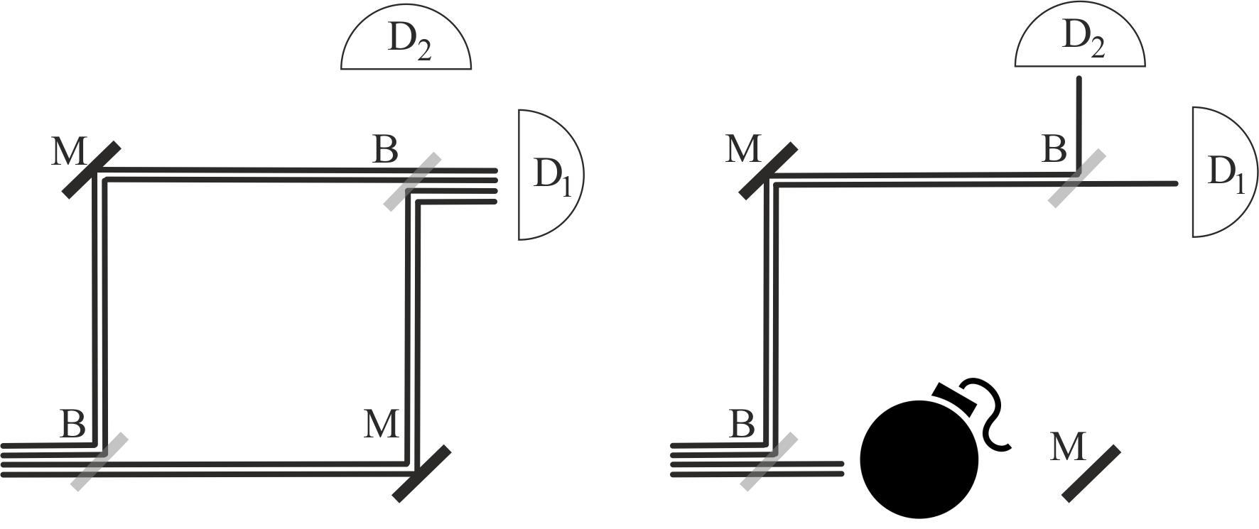
Figure 3: Sketch of the bomb experiment with Bohmian trajectories. Black bars marked M are mirrors, semi-transparent grey bars marked B are beam-splitters. One of the trajectories on the upper path needs to change direction on the second beam splitter when a live bomb is put into place (or a which-path measurement is made on the lower path, respectively).

This reveals that one of the the Bohmian trajectories on the path without the bomb must do two different things at the second beam splitter, depending on what one measures. This makes sense because we have to interpret the bomb as a detector which effectively decoheres the incoming part of the pilot wave. It can then no longer recombine with the upper path to cancel out the wave going to detector D₂. That is, in Bohmian mechanics the pilot wave “feels out” the path with the bomb even though the Bohmian particle does not go there.

This example however does not require non-locality because there’s only one particle involved and so the paths recombine at the second beam splitter. To get an example that requires non-locality, we could use a Bell-type experiment with spin measurements. However, the treatment of spin in Bohmian Mechanics is somewhat controversial.

We will therefore instead use an example previously proposed in [72]. It is a modified version of the quantum eraser experiment [73, 74], in which the two different spin states of a Bell-experiment are represented as two different paths. This example has the benefit of revealing the non-locality visually because the paths are both different, whereas in the usual Bell experiments the different spins states all go on the same path.

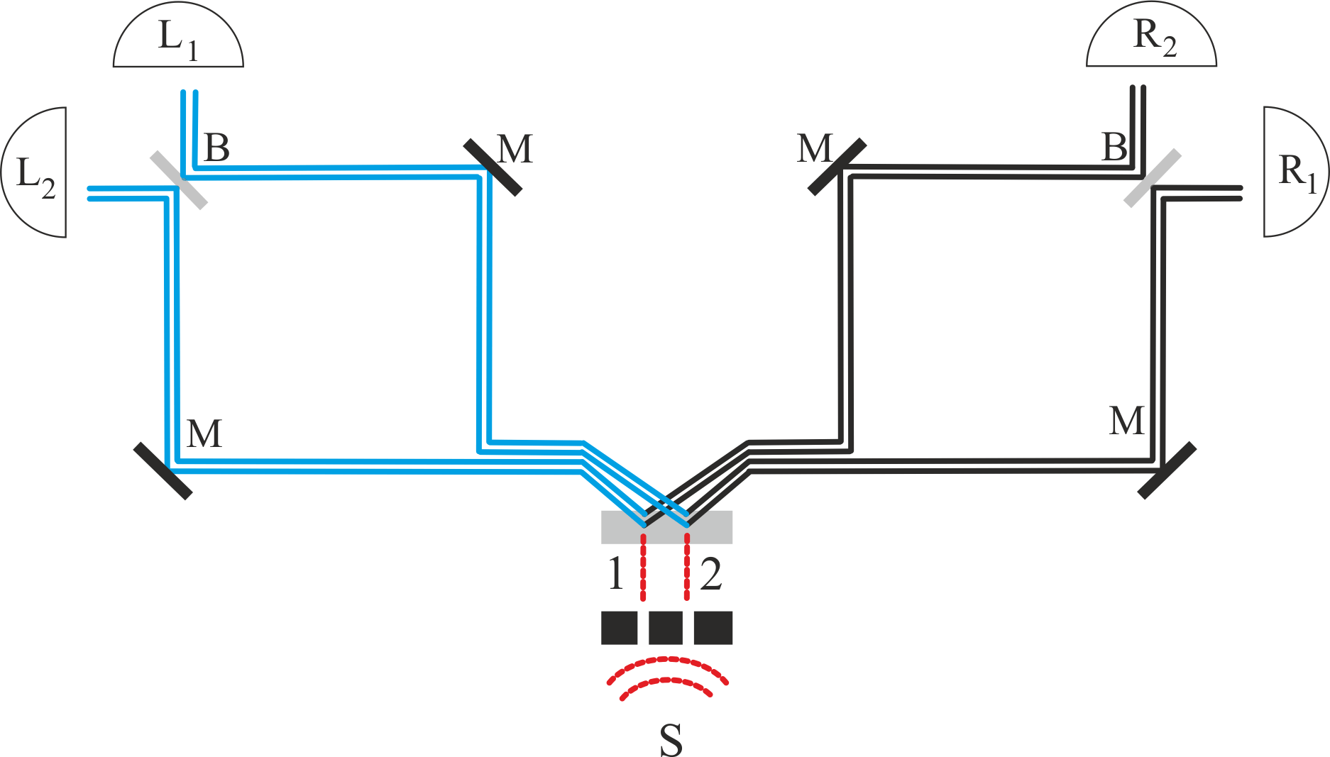
Figure 4: Sketch of the modified eraser experiment with Bohmian trajectories.

In this experiment (Figure 4), photons are emitted from a single photon source (S) and sent through a double slit (black). After the double-slit, the photons hit a nonlinear optical crystal (light grey) which, by spontaneous parametric down conversion, creates an entangled pair of photons from each photon incident on the crystal. Note that this creates two new particles (lines in black and blue, respectively). Trajectories of Bohmian particles belonging to different photons can cross because they obey different differential equations.

The photon pairs which emerge from the optical crystal are phase-matched and we denote them with $|{\rm 1}\rangle=(1,0)^{\rm T}$ and $|{\rm 2}\rangle=(0,1)^{\rm T}$, depending on which slit they came from. The photons on each side then each enter a Mach-Zehnder interferometer lacking the first beam splitter, with paths adjusted so that photon counts are the same in L₁ and L₂, or R₁ and R₂, respectively.

In this setup, the location at which the entangled particles are created (1 or 2) imprints the information that is later erased when the states are mixed at the beam splitters. The erasure then comes down to the somewhat unremarkable statement that if we measure one of the entangled particles in L₁ (L₂), then its partner goes to R₁ (R₂).

But on both paths of the entangled photons we can alternatively chose to measure the which path information with detectors we will call R_3/4 and L_3/4 (not shown in Figure). If we measure a combination of L_1/2 and R_3/4 (or the other way round), they should not be correlated at all.

We adopt the convention that the first entry in the product state denotes the photon going left, the second the photon going right. Then the state after the crystal can be written as

$$|\Psi\rangle = \frac{1}{\sqrt{2}}\Big{(}|{\rm 1}\rangle_{\rm L}|{\rm 1}\rangle_{\rm R}+|{\rm 2}\rangle_{\rm L}|{\rm 2}\rangle_{\rm R}\Big{)}$$ (14)

$$= \frac{1}{\sqrt{2}}\Big{(}|-\rangle_{\rm L}|-\rangle_{\rm R}+|+\rangle_{\rm L}|+\rangle_{\rm R}\Big{)}~{}.$$ (15)

where

$$|\pm\rangle_{\rm L/R}:=\frac{1}{\sqrt{2}}\left(|1\rangle_{\rm L/R}\pm|2\rangle_{\rm L/R}\right)~{}.$$ (16)

The actions of the which-path detectors are

$${\rm L}_{3}:|1\rangle_{\rm L}\langle{\rm 1}|_{\rm L}\otimes{\rm\mathds{1}}_{\rm R}~{},~{}{\rm L}_{4}:|{\rm 2}\rangle_{\rm L}\langle{\rm 2}|_{\rm L}\otimes{\rm\mathds{1}}_{\rm R}~{},$$

$${\rm R}_{3}:{\rm\mathds{1}}_{\rm L}\otimes|1\rangle_{\rm R}\langle{1}|_{\rm R}~{},~{}{\rm R}_{4}:{\rm\mathds{1}}_{\rm L}\otimes|2\rangle_{\rm R}\langle{\rm 2}|_{\rm R}~{}.$$ (17)

The detectors L_1/2 and R_1/2 instead project on the bases rotated by the action of the beam splitter $B$ so that

$${\rm L}_{1}:|-\rangle_{\rm L}\langle-|_{\rm L}\otimes{\rm\mathds{1}}_{\rm R}~{},~{}{\rm L}_{2}:|{\rm+}\rangle_{\rm L}\langle{\rm+}|_{\rm L}\otimes{\rm\mathds{1}}_{\rm R}~{},$$

$${\rm R}_{1}:{\rm\mathds{1}}_{\rm L}\otimes|{\rm-}\rangle_{\rm R}\langle{\rm-}|_{\rm R}~{},~{}{\rm R}_{2}:{\rm\mathds{1}}_{\rm L}\otimes|{\rm+}\rangle_{\rm R}\langle{\rm+}|_{\rm R}~{}.$$ (18)

This setup is basically a double bomb-experiment (the which-path detectors playing the role of the bomb), so we can draw on our insights about Bohmian trajectories in the single-bomb experiment. The relevant difference is that in the double-bomb setup, a which-path measurement on one of the two entangled photons now must influence the Bohmian trajectory of the other photon (for an example, see Figure 5). And the other photon could be arbitrarily far away. Hence, non-locality is required in Bohmian Mechanics to explain the measurement results.

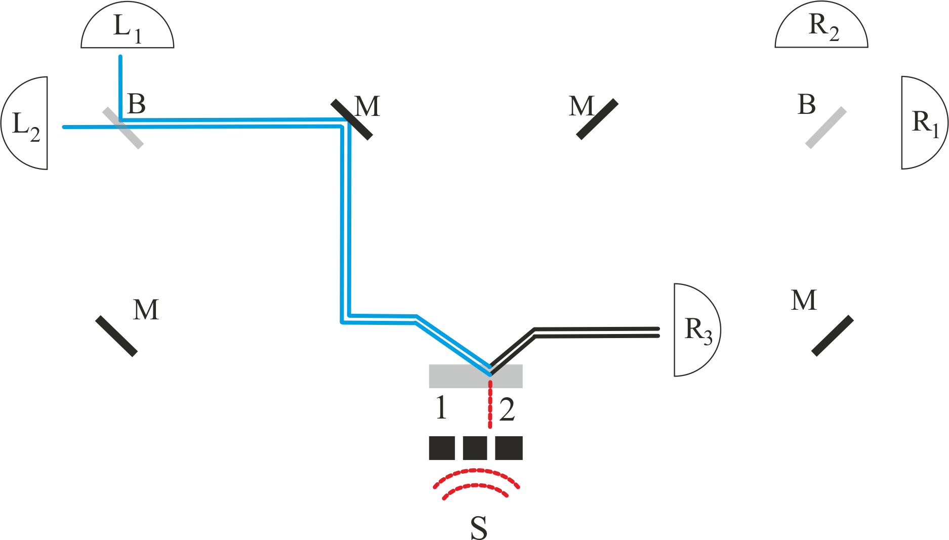
Figure 5: Sketch to illustrate how a which-way measurement on the right side must change the Bohmian trajectories on the left side, which could be causally disconnected.

I am telling you this because it shows that while Bohmian Mechanics violates Measurement Independence, it does so because (a) the paths of the Bohmian particles must depend on what is usually called the measurement setting, and (b) the paths non-locally influence each other via the velocity equation. That is, the non-locality is the origin of the violation of Measurement Independence. Though it is eventually a matter of nomenclature, for me this example illustrates that it makes no sense to define superdeterminism by merely a lack of Measurement Independence. One also needs to require locality, for non-locality can easily induce violations of Measurement Independence. It would be confusing to lump Bohmian Mechanics together with models that employ violations of Measurement Independence to restore Local Causality.

This example is also useful to address another common misunderstanding, which is that a violation of Measurement Independence in a hidden variables theory is a statement about the initial conditions for the hidden variables. If we generally denote the hidden variables with $\lambda$ and the detector settings (of possibly several detectors) with $X$, then a violation of Measurement Independence means $\rho(\lambda|X)\neq\rho(\lambda)$, where $\rho$ is the probability density of the hidden variables. This probability density is usually interpreted as one at the time of preparation of the system (see e.g. [75]).

However, as pointed out in [18], the quantity $\rho(\lambda)$ appears in Bell’s theorem to calculate the measurement result. Initial values for the hidden variables without an evolution law are not sufficient for that. Hence, the $\lambda$s in Bell’s theorem must necessarily include information about the evolution law and Measurement Independence can be violated by the evolution law, rather than by the initial condition. This is exactly what happens in Bohmian Mechanics.

The initial condition of the particles in Bohmian mechanics does not depend on the measurement settings as it is just a way of re-expressing the initial state of the wave-function in the Copenhagen Model. But since in Bohmian Mechanics the only quantity that can be measured is the position of the Bohmian particles, the quantity that is normally called the measurement setting must become part of the evolution law. If one correctly identifies the hidden variables as the combination of initial state and evolution law, one sees that Measurement Independence must be violated.

6.3 Measurements in Bohmian Mechanics

Let us then look at what Bohmian Mechanics has to say about the measurement problem.

We already saw that Bohmian Mechanics is non-local, so it does not solve that aspect of the measurement problem. But what about the other aspect of the measurement problem, that which explains what makes a collection of particles act as a measurement device? Well, in Bohmian Mechanics there is no need for an apparatus to bring a state into an eigenstate of the operator that describes the measurement variable because the only thing that can be measured in in this model is the position of the Bohmian particles, and this position always has a definite value anyway. That is, this part of the measurement problem doesn’t exist in Bohmian Mechanics for the same reason it doesn’t exist in classical mechanics.

In a classical theory we have no problem with explaining why, say, a thermometer tells us the temperature of a system, because that’s just a consequence of the interaction between the thermometer and the system we are interested in. This works because the system has a temperature whether or not we measure it and we just need to read it out. True, we often don’t write down this interaction between the measurement device and the system in detail, but we know how it works in principle.

This is not the case in the Copenhagen Model, where the prepared state a priori simply does not have a definite value for the variable we want to measure (because it’s in a superposition), and the interaction between the system and the measurement device is a unitary transformation that just maintains those superpositions. It is for this reason that, in the Copenhagen Model, the measurement device needs to somehow make the measurement variable definite by “collapsing” superpositions. But in Bohmian Mechanics this is not necessary. It is therefore not so much that Bohmian Mechanics solves the problem as that it doesn’t have it to begin with.

The measurement process in Bohmian mechanics itself works similar to decoherence, in that one regards the system of prepared state plus the detector and the environment. Then one effectively removes the environment and detector by creating what is called the “conditional wave-function”, by inserting the positions of the Bohmian particles that one is not interested in. The remaining wave-function then effectively contracts the probability distribution which can be interpreted as a sort of collapse. However, much like in decoherence approaches, this idea requires one to know already that a collection of particles will act as a measuring device.

So does Bohmian Mechanics solve the part of the measurement problem that pertains the identification of what constitutes a detector? It does so as much or as little as decoherence and the Many Worlds Interpretation do. That is, if one designates part of the state as detector and environment, then one can create a conditional wave-function for the prepared state that evolves into a position eigenstate, but one does not know from the initial state alone what constitutes the detector and its environment.

7 Discussion

As always there is more that could be said. For example, to me the above discussion raises the question whether temporal determinism is even a meaningful criterion, given how easily it can be re-established by positing mathematical entities (be that disconnected parallel worlds or particles with unknowable positions) that are unmeasurable, even in principle. Another interesting question is why Bohmian Mechanics needs to violate Local Causality when it also violates Measurement Independence. It seems to me that either it doesn’t actually violate Local Causality, or it must be possible to find a modified, yet empirically equivalent, version that does respect Local Causality.

Finally, I would like to submit that I have no personal preference for either of these interpretations of quantum mechanics. To me they are all equally useful and equally unsatisfactory. I merely hope that this modest contribution to the literature will help identify just what is unsatisfactory about them.

8 Summary

In summary, I have applied an instrumentalist approach to explain why both the Many Worlds Interpretation and Bohmian Mechanics are non-local and solve the measurement problem only partially, just like the Copenhagen Interpretation.

References

- [1] Emily Adlam, Jonte Hance, Sabine Hossenfelder, and Tim Palmer. Taxonomy for physics beyond quantum mechanics. arXiv preprint xxxx.yyyy, 2023. URL: https://arxiv.org/abs/xxxx.yyyy.
- [2] Wojciech Hubert Zurek. Quantum theory of the classical: quantum jumps, Born’s rule and objective classical reality via quantum Darwinism. Philosophical Transactions of the Royal Society A: Mathematical, Physical and Engineering Sciences, 376(2123):20180107, 2018. doi:10.1098/rsta.2018.0107.
- [3] Leslie E Ballentine. The statistical interpretation of quantum mechanics. Reviews of modern physics, 42(4):358, 1970. doi:10.1103/RevModPhys.42.358.
- [4] Lucien Hardy. Quantum theory from five reasonable axioms. arXiv preprint quant-ph/0101012, 2001.
- [5] Scott Aaronson. Is quantum mechanics an island in theoryspace? arXiv preprint quant-ph/0401062, 2004.
- [6] Andrew M Gleason. Measures on the closed subspaces of a hilbert space. In The Logico-Algebraic Approach to Quantum Mechanics: Volume I: Historical Evolution, pages 123–133. Springer, 1975.
- [7] David Deutsch. Quantum theory of probability and decisions. Proceedings of the Royal Society of London. Series A: Mathematical, Physical and Engineering Sciences, 455(1988):3129–3137, 1999.
- [8] Borivoje Dakic and Caslav Brukner. Quantum theory and beyond: Is entanglement special? arXiv preprint arXiv:0911.0695, 2009.
- [9] Lev Vaidman. Probability in the many-worlds interpretation of quantum mechanics. In Probability in physics, pages 299–311. Springer, 2011.
- [10] Charles T Sebens and Sean M Carroll. Self-locating uncertainty and the origin of probability in everettian quantum mechanics. The British Journal for the Philosophy of Science, 2018.
- [11] Sabine Hossenfelder. A derivation of born’s rule from symmetry. Annals of Physics, 425:168394, 2021.
- [12] John S Bell. The theory of local beables. Technical Report CERN-TH-2053, CERN, 1975.
- [13] Travis Norsen. Local causality and completeness: Bell vs. jarrett. Foundations of Physics, 39(3):273–294, 2009.
- [14] John S Bell. On the Einstein Podolsky Rosen paradox. Physics Physique Fizika, 1(3):195, 1964. doi:10.1103/PhysicsPhysiqueFizika.1.195.
- [15] A. Einstein, B. Podolsky, and N. Rosen. Can quantum-mechanical description of physical reality be considered complete? Phys. Rev., 47:777–780, May 1935. doi:10.1103/PhysRev.47.777.
- [16] Sabine Hossenfelder and Tim Palmer. Rethinking superdeterminism. Frontiers in Physics, 8:139, 2020. doi:10.3389/fphy.2020.00139.
- [17] Sabine Hossenfelder. Superdeterminism: A guide for the perplexed. arXiv preprint arXiv:2010.01324, 2020. URL: https://arxiv.org/abs/2010.01324.
- [18] Jonte R. Hance and Sabine Hossenfelder. The wave function as a true ensemble. Proceedings of the Royal Society A, 478:20210705, 2022. doi:10.1098/rspa.2021.0705.
- [19] Roderich Tumulka. Bohmian mechanics. arXiv preprint arXiv:1704.08017, 2021.
- [20] Avshalom C. Elitzur and Lev Vaidman. Quantum mechanical interaction-free measurements. Foundations of Physics, 23(7):987–997, Jul 1993. doi:10.1007/BF00736012.
- [21] Onur Hosten, Matthew T Rakher, Julio T Barreiro, Nicholas A Peters, and Paul G Kwiat. Counterfactual quantum computation through quantum interrogation. Nature, 439(7079):949–952, 2006.
- [22] Tim Maudlin. Three measurement problems. topoi, 14(1):7–15, 1995.
- [23] AJ Leggett. The quantum measurement problem. science, 307(5711):871–872, 2005. doi:10.1126/science.1109541.
- [24] Jonte R Hance and Sabine Hossenfelder. What does it take to solve the measurement problem? Journal of Physics Communications, 6(10):102001, 2022.
- [25] Wojciech Hubert Zurek. Decoherence, einselection, and the quantum origins of the classical. Rev. Mod. Phys., 75:715–775, May 2003. URL: https://link.aps.org/doi/10.1103/RevModPhys.75.715, doi:10.1103/RevModPhys.75.715.
- [26] Maximilian Schlosshauer. Decoherence, the measurement problem, and interpretations of quantum mechanics. Rev. Mod. Phys., 76:1267–1305, Feb 2005. doi:10.1103/RevModPhys.76.1267.
- [27] Ruth E. Kastner. ‘Einselection’ of pointer observables: The new H-theorem? Studies in History and Philosophy of Science Part B: Studies in History and Philosophy of Modern Physics, 48:56–58, 2014. doi:10.1016/j.shpsb.2014.06.004.
- [28] Maximilian Schlosshauer. Quantum decoherence. Physics Reports, 831:1–57, 2019.
- [29] infinitelylarge. Quantum wave functions do not collapse, Jan. 2020. URL: https://www.youtube.com/watch?v=GpnLMaWylp4.
- [30] Hugh Everett III. ” relative state” formulation of quantum mechanics. Reviews of modern physics, 29(3):454, 1957.
- [31] Bryce S DeWitt. Quantum mechanics and reality. Physics today, 23(9):30–35, 1970.
- [32] H Dieter Zeh. On the interpretation of measurement in quantum theory. Foundations of Physics, 1:69–76, 1970.
- [33] David Deutsch. Quantum theory as a universal physical theory. International Journal of Theoretical Physics, 24:1–41, 1985.
- [34] James B Hartle. Spacetime coarse grainings in nonrelativistic quantum mechanics. Physical Review D, 44(10):3173, 1991.
- [35] Michael Lockwood. ’many minds’. interpretations of quantum mechanics. The British journal for the philosophy of science, 47(2):159–188, 1996.
- [36] Carlo Rovelli. Relational quantum mechanics. International Journal of Theoretical Physics, 35(8):1637–1678, 1996. doi:10.1007/BF02302261.
- [37] Simon Saunders and David Wallace. Branching and uncertainty. The British Journal for the Philosophy of Science, 2008.
- [38] Sean M Carroll and Charles T Sebens. Many worlds, the born rule, and self-locating uncertainty. In Quantum theory: A two-time success story: Yakir Aharonov Festschrift, pages 157–169. Springer, 2014.
- [39] Christian List. The many-worlds theory of consciousness. Noûs, 57(2):316–340, 2023.
- [40] Mordecai Waegell and Kelvin J McQueen. Reformulating bell’s theorem: The search for a truly local quantum theory. Studies in History and Philosophy of Science Part B: Studies in History and Philosophy of Modern Physics, 70:39–50, 2020.
- [41] Aurélien Drezet. An elementary proof that everett’s quantum multiverse is nonlocal: Bell-locality and branch-symmetry in the many-worlds interpretation. Symmetry, 15(6):1250, 2023.
- [42] David Wallace. The emergent multiverse: Quantum theory according to the Everett interpretation. Oxford University Press, USA, 2012.
- [43] Kelvin J McQueen and Lev Vaidman. In defence of the self-location uncertainty account of probability in the many-worlds interpretation. Studies in History and Philosophy of Science Part B: Studies in History and Philosophy of Modern Physics, 66:14–23, 2019.
- [44] Daniela Frauchiger and Renato Renner. Quantum theory cannot consistently describe the use of itself. Nature communications, 9(1):3711, 2018.
- [45] David Bohm. A suggested interpretation of the quantum theory in terms of ”hidden” variables. i. Phys. Rev., 85:166–179, Jan 1952. doi:10.1103/PhysRev.85.166.
- [46] David Bohm. A suggested interpretation of the quantum theory in terms of ”hidden” variables. ii. Phys. Rev., 85:180–193, Jan 1952. doi:10.1103/PhysRev.85.180.
- [47] Lucien Hardy. On the existence of empty waves in quantum theory. Physics Letters A, 167(1):11–16, 1992.
- [48] Enrico Deotto and GianCarlo Ghirardi. Bohmian mechanics revisited. Foundations of Physics, 28:1–30, 1998.
- [49] Peter J Lewis. Empty waves in bohmian quantum mechanics. The British journal for the philosophy of science, 2007.
- [50] Detlef Dürr, Sheldon Goldstein, and Nino Zanghi. Bohmian mechanics as the foundation of quantum mechanics. Bohmian mechanics and quantum theory: an appraisal, pages 21–44, 1996.
- [51] Detlef Dürr, Sheldon Goldstein, and Nino Zanghi. Quantum equilibrium and the origin of absolute uncertainty. Journal of Statistical Physics, 67:843–907, 1992.
- [52] Euan J Squires. A local hidden-variable theory that, fapp, agrees with quantum theory. Physics Letters A, 178(1-2):22–26, 1993. doi:10.1016/0375-9601(93)90721-B.
- [53] Karin Berndl, Detlef Dürr, Sheldon Goldstein, and Nino Zanghì. Nonlocality, lorentz invariance, and bohmian quantum theory. Physical Review A, 53(4):2062, 1996. doi:10.1103/PhysRevA.53.2062.
- [54] Detlef Dürr, Sheldon Goldstein, Karin Münch-Berndl, and Nino Zanghì. Hypersurface bohm-dirac models. Physical Review A, 60(4):2729, 1999. doi:10.1103/PhysRevA.60.2729.
- [55] George Horton and Chris Dewdney. A non-local, lorentz-invariant, hidden-variable interpretation of relativistic quantum mechanics based on particle trajectories. Journal of Physics A: Mathematical and General, 34(46):9871, 2001. doi:10.1088/0305-4470/34/46/310.
- [56] Chris Dewdney and George Horton. Relativistically invariant extension of the de broglie–bohm theory of quantum mechanics. Journal of Physics A: Mathematical and General, 35(47):10117, 2002. doi:10.1088/0305-4470/35/47/311.
- [57] George Horton and Chris Dewdney. A relativistically covariant version of bohm’s quantum field theory for the scalar field. Journal of Physics A: Mathematical and General, 37(49):11935, 2004. doi:10.1088/0305-4470/37/49/011.
- [58] Detlef Dürr, Sheldon Goldstein, Roderich Tumulka, and Nino Zanghi. Bohmian mechanics and quantum field theory. Physical Review Letters, 93(9):090402, 2004. doi:10.1103/PhysRevLett.93.090402.
- [59] Hrvoje Nikolić. Relativistic quantum mechanics and the bohmian interpretation. Foundations of Physics Letters, 18(6):549–561, 2005. doi:10.1007/s10702-005-1128-1.
- [60] Hrvoje Nikolic. Many-fingered time bohmian mechanics. arXiv preprint quant-ph/0603207, 2006. URL: https://arxiv.org/abs/quant-ph/0603207.
- [61] Samuel Colin and Ward Struyve. A dirac sea pilot-wave model for quantum field theory. Journal of Physics A: Mathematical and Theoretical, 40(26):7309, 2007. doi:10.1088/1751-8113/40/26/015.
- [62] Ward Struyve. Pilot-wave theory and quantum fields. Reports on Progress in Physics, 73(10):106001, 2010. doi:10.1088/0034-4885/73/10/106001.
- [63] Detlef Dürr, Sheldon Goldstein, Travis Norsen, Ward Struyve, and Nino Zanghì. Can bohmian mechanics be made relativistic? Proceedings of the Royal Society A: Mathematical, Physical and Engineering Sciences, 470(2162):20130699, 2014. doi:10.1098/rspa.2013.0699.
- [64] Antony Valentini. Signal-locality, uncertainty, and the subquantum H-theorem. I. Physics Letters A, 156(1):5–11, 1991. doi:10.1016/0375-9601(91)90116-P.
- [65] Antony Valentini. Signal-locality, uncertainty, and the subquantum H-theorem. II. Physics Letters A, 158(1):1–8, 1991. doi:10.1016/0375-9601(91)90330-B.
- [66] Hrvoje Nikolic. Time and probability: From classical mechanics to relativistic bohmian mechanics. arXiv preprint arXiv:1309.0400, 2013.
- [67] Lucien Hardy. Contextuality in bohmian mechanics. In Bohmian mechanics and quantum theory: An appraisal, pages 67–76. Springer, 1996.
- [68] Marian Kupczynski. Contextuality or Nonlocality: What Would John Bell Choose Today? Entropy, 25(2):280, 2023. arXiv:2202.09639, doi:10.3390/e25020280.
- [69] John G Cramer. The transactional interpretation of quantum mechanics. Reviews of Modern Physics, 58(3):647, 1986. doi:10.1103/RevModPhys.58.647.
- [70] John G Cramer. The transactional interpretation of quantum mechanics and quantum nonlocality. arXiv preprint arXiv:1503.00039, 2015.
- [71] Ruth E Kastner. The transactional interpretation of quantum mechanics: the reality of possibility. Cambridge University Press, 2013.
- [72] Colm Bracken, Jonte R Hance, and Sabine Hossenfelder. The quantum eraser paradox. arXiv preprint arXiv:2111.09347, 2021.
- [73] Marlan O Scully and Kai Drühl. Quantum eraser: A proposed photon correlation experiment concerning observation and” delayed choice” in quantum mechanics. Physical Review A, 25(4):2208, 1982. doi:10.1103/PhysRevA.25.2208.
- [74] Yoon-Ho Kim, Rong Yu, Sergei P Kulik, Yanhua Shih, and Marlan O Scully. Delayed “choice” quantum eraser. Physical Review Letters, 84(1):1, 2000. doi:10.1103/PhysRevLett.84.1.
- [75] Matthew F Pusey, Jonathan Barrett, and Terry Rudolph. On the reality of the quantum state. Nature Physics, 8(6):475–478, 2012. doi:10.1038/NPHYS2309.