Checking the second law at cosmic scales

Abstract

Based on recent data about the history of the Hubble factor, it is argued that the second law of thermodynamics holds at the largest scales accessible to observation. This is consistent with previous studies of the same question.

1 Introduction

The second law of thermodynamics is one of the pillars of our understanding the physical world. According to this law, isolated macroscopic systems tend to a state of thermodynamic equilibrium compatible with the constraints of the system itself. The equilibrium is characterized by a state of maximum entropy, which means that, for isolated systems, the latter never decreases but eventually attains a maximum at equilibrium. On the other hand, experience and common sense tell us that it will never increase unbounded.

The common lore says that, nowadays, the entropy of the Universe (i.e., that part of the Universe in causal contact with us) is strongly dominated by the entropy of the cosmic horizon, $S_{h}$, nearly $10^{122}$ times the Boltzmann constant. The other main sources of entropy (e.g. supermassive black holes, the cosmic background radiation, the cosmic sea of neutrinos, etc.) contribute less by many orders of magnitude [1].

As is well known, the second law is fulfilled at terrestrial scales and it is routinely applied at solar and galactic scales. Further, to the best of our knowledge, all attempts to disprove it have failed. However, it remains to be seen if it is also satisfied at the largest scales accessible to observation; i.e., at cosmic scales. Nevertheless, a recent study suggests that this is indeed the case [2]. The target of this research is to check whether the second law is satisfied at the aforementioned scales by a different method that in Ref. [2]. In the latter, three different and reasonable parametrizations of the Hubble function were employed. By contrast we do not resort to any parametrization; instead we use a well known expression of the current spatial curvature parameter (Eq. (3.2), below) that holds at any time under consideration.

We resort to recent cosmological data on the history of the Hubble parameter; namely, cosmic chronometers (CC) measurements, baryon acoustic oscillations (BAO), and luminosity distances from type Ia supernovae (SNIa) (32, 8 and 1624 data points, respectively). These data are affected by the respective statistical and systematic uncertainties whereby to obtain a sensible graph of the said history we apply Gaussian processes [3] to smooth the data, a widely used technique in physical cosmology (see, e.g. [4, 5]). Our only assumptions are the validity of Einstein gravity and that at sufficiently large scales the Universe is spatially homogeneous and isotropic, faithfully described by the Robertson-Walker metric.

Given that $S_{h}\propto{\cal A}$, where ${\cal A}=\frac{\pi}{H^{2}+ka^{-2}}$ is the area of the apparent horizon [6], $a$ being the scale factor and $H\equiv\dot{a}/a$ the Hubble function, the second law implies that ${\cal A}$ cannot decrease with the expansion. As it turns out we found that $d{\cal A}/da\geq 0$, or equivalently $d{\cal A}/dz\leq 0$ in the redshift range, $0<z\leq 2$, considered and thereby the second law is fulfilled in the said range.

The manuscript is organized as follows. In section 2, we write the cosmic scales in terms of the deceleration parameter $q$ and curvature density parameter $\Omega_{k}$. The methodology adopted is discussed in section 3. Section 4 introduces the observational data sets, followed by a brief description of the Gaussian process algorithm, and the final reconstruction. We investigate the validity of the second law at cosmic scales from the results in section 5. Finally, in section 6 we summarize our findings and make some concluding remarks.

2 Theoretical Framework

It is straightforward to see that the second law of thermodynamics can alternatively be written as

$$1+q\geq\Omega_{k}\,,$$ (2.1)

where $q\equiv-\ddot{a}/(aH^{2})$ is the deceleration parameter and $\Omega_{k}\equiv-k/(aH)^{2}$ the spatial curvature parameter. Obviously this expression necessarily holds when the universe is decelerating ($q>0$) or coasting ($q=0$), since because of the Friedmann equation $\mid\Omega_{k}\mid\leq 1$. However, for accelerating ($q<0$) the said expression could be violated, at least in principle. Here we propose a novel experimental method to check whether if this is the case.

From the above definition of spatial curvature it follows

$$\Omega_{k}(z)=\Omega_{k0}\frac{(1+z)^{2}}{E^{2}(z)},$$ (2.2)

where $E(z)=H(z)/H_{0}$ is the normalized, dimensionless, Hubble factor.

Noting that $1+q=-\dot{H}/H^{2}=(1+z)\frac{H^{\prime}}{H}$, the second law can be recast as

$$H^{\prime}(z)\geq\Omega_{k0}\,H_{0}^{2}\,\frac{1+z}{H(z)},$$ (2.3)

where a prime means differentiation with respect to redshift.

The latter sets a lower bound on the slope of the graph of the Hubble function versus redshift. Here we wish to check the validity of this inequality using updated observational data on the history of the Hubble factor. These included Hubble parameter measurements from CC, BAO, and luminosity distance measurements from SNIa.

The luminosity distance of any object (such as supernovae), is given by

$$d_{L}{}=\frac{c(1+z)}{H_{0}\sqrt{\mid\Omega_{k0}\mid}}\,{\rm sinn}\left[\sqrt{\mid\Omega_{k0}\mid}\,\int_{0}^{z}{\frac{d\tilde{z}}{E(\tilde{z})}}\right],$$ (2.4)

where ${\rm sinn}[x]$ is $\sinh(x),x$ and $\sin(x)$ for positive, zero and negative spatial curvature, respectively, and $c$ is the speed of light. We define the transverse comoving distance to the source as,

$$d_{C}(z)=\frac{d_{L}}{1+z},$$ (2.5)

and,

$$D(z)=\frac{H_{0}}{c}d_{C}(z)$$ (2.6)

is the normalized comoving distance.

3 Methodology

To investigate the validity of the second law of thermodynamics one needs to obtain constraints on the parameter of spatial curvature. Equation (2.3) amounts to the following condition

$$\zeta\equiv H^{\prime}(z)-\Omega_{k0}\,H_{0}^{2}\,\,\frac{1+z}{H(z)}\geq 0,$$ (3.1)

for the non-violation of the second law of thermodynamics.

Now, given an estimate for the combination $\Omega_{k0}H_{0}^{2}$, one can directly obtain $\zeta$ from Eq. (3.1).

Alternatively, one can reconstruct the curvature density parameter by exploiting the relation

$$\Omega_{k0}=\frac{E^{2}(z)\,D^{\prime 2}(z)-1}{D^{2}(z)}=\frac{H^{2}(z)\,d_{C}^{\prime 2}(z)-c^{2}}{H_{0}^{2}~{}d_{C}^{2}(z)},$$ (3.2)

which comes directly from Eq. (2.4), see e.g. [7, 8].

From equations (2.3), (3.2) and the inequality, (3.1), we get

$$\zeta\equiv H^{\prime}(z)-\frac{(1+z)}{H(z)}\,\frac{[H^{2}(z)\,d_{C}^{\prime 2}(z)-c^{2}]}{d_{C}^{2}(z)}\geq 0.$$ (3.3)

This is independent of any specific cosmological model; it solely rests on the Robertson-Walker metric.

The inequality (2.1) holds for decelerating and coasting universes. It is found to be satisfied at the present epoch for all types of spatial curvature ($k=0,+1,-1$) as well (see Mukherjee and Banerjee [9]); however, it is not guaranteed that it will hold at all intermediate redshifts. If experimentally it is proved valid also between the commencement of the accelerated phase of cosmic expansion (around a redshift of $0.78$, see e.g. [10]) and the present, it will strongly support the idea that the second law applies to the observable universe and that the latter behaves as a thermodynamic system. As mentioned above, solid arguments in favor of this idea have been put forward in Ref. [2] based on the history of the Hubble factor and reasonable parametric expressions of the latter.

However, though we utilize $H(z)$ data as well, our method differs from theirs in that we do not resort to any parametrization of the Hubble parameter. Instead we implement a non-parametric reconstruction of the spatial curvature parameter (3.2), or directly utilize model-independent $\Omega_{k0}H_{0}^{2}$ constraints (2.3) from the Hubble and supernova datasets.

4 Reconstruction

Data-driven reconstruction is being widely used for model-independent predictions in cosmology. Here, we resort to the machine-learning algorithm, Gaussian process (GP) regression [4, 5], which can infer a function from a labeled set of training data. Any function obtained from a GP is characterized by some mean and covariance function. The prior mean function has been set to zero. So, the covariance function or ‘kernel’, plays the central role in encoding correlations between points where no data are available. Therefore, this process can reproduce an ample range of behaviors and allows a Bayesian interpretation. A wide variety of covariance functions exists in the literature. For this work, we consider six different kernels, namely,

A. Squared Exponential (RBF)

$$\kappa(z,\tilde{z})=\sigma_{f}^{2}\,\exp\left[-\frac{(z-\tilde{z})^{2}}{2l^{2}}\right]\,,$$ (4.1)

B. Rational Quadratic (RQD)

$$\kappa(z,\tilde{z})=\sigma_{f}^{2}\,\left[1+\frac{(z-\tilde{z})^{2}}{2\alpha l^{2}}\right]^{-\alpha}\,,$$ (4.2)

C. Cauchy (CHY)

$$\kappa(z,\tilde{z})=\sigma_{f}^{2}\,\left[\frac{l}{(z-\tilde{z})^{2}+l^{2}}\right]\,,$$ (4.3)

D. Matérn with $\nu=\frac{5}{2}$ (M52), $\nu=\frac{7}{2}$ (M72), $\nu=\frac{9}{2}$ (M92)

$$\kappa(z,\tilde{z})=\sigma_{f}^{2}\,\frac{{\left[\frac{\sqrt{2\nu}}{l}\,(z-\tilde{z})\right]}^{\nu}}{\Gamma(\nu)\,2^{\nu-1}}\,K_{\nu}\left(\frac{\sqrt{2\nu}}{l}(z-\tilde{z})\right)\,,$$ (4.4)

where $\nu$ denotes the order, $K_{\nu}(\cdot)$, and $\Gamma(\cdot)$ are the modified Bessel and Gamma functions. The kernel hyperparameters, $\sigma_{f}$, $l$ and $\alpha$, typically control the strength of the fluctuations, the correlation length and the relative weighting of large-scale and small-scale variations at different length scales, between two separate redshifts.

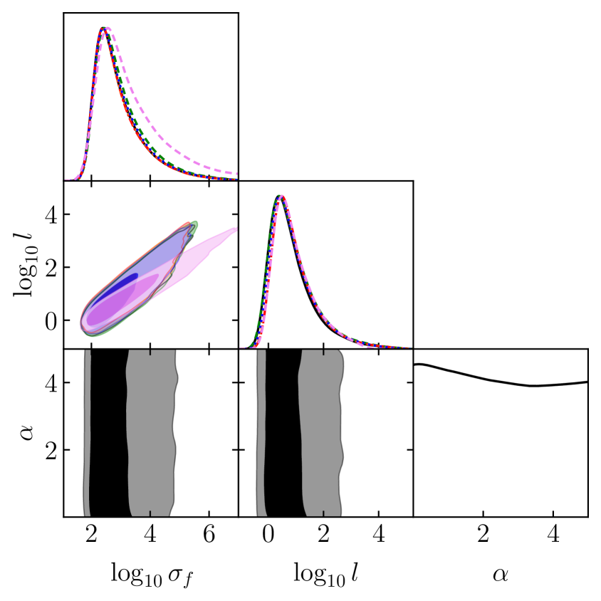
(a) CC

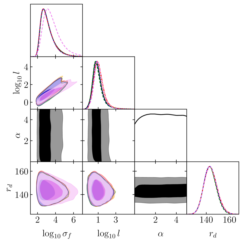
(b) CC+BAO

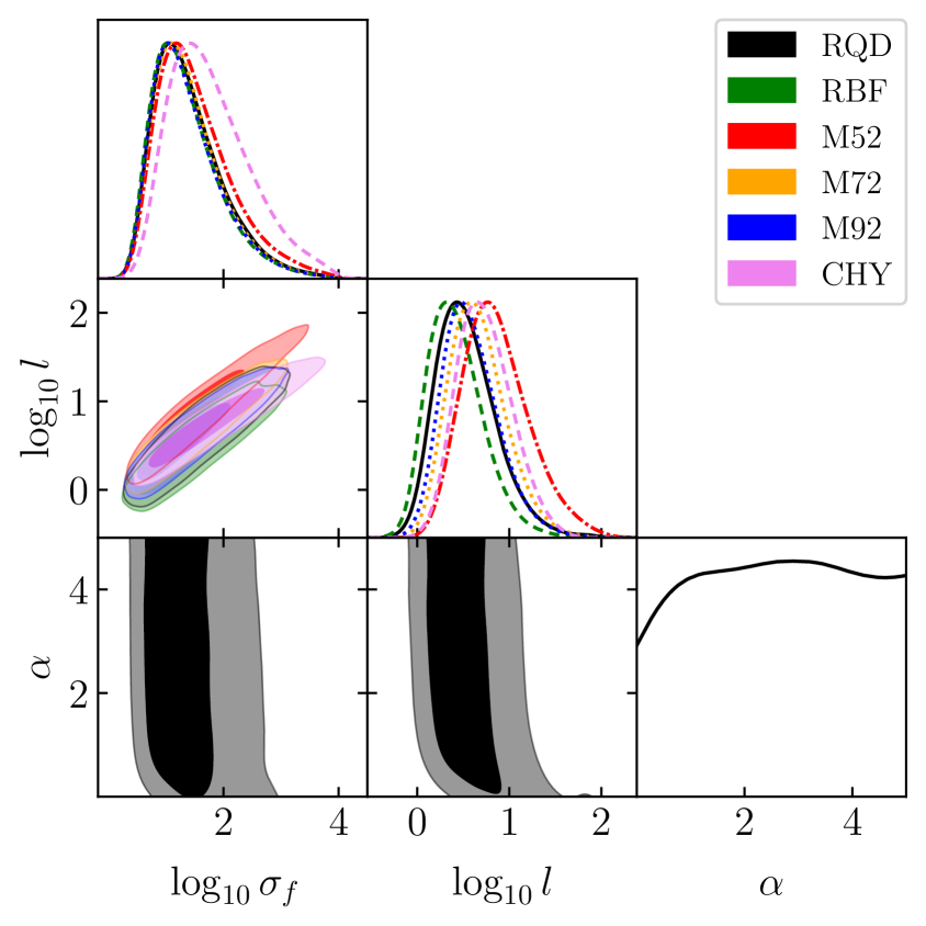
(c) SN

Figure 1: Contour for GP hyperparameter space and the comoving sound horizon radius at drag epoch, $r_{d}$ [in units of Mpc], using different choices of the GP kernels.

$\kappa(z,\tilde{z})$	$M$	$\Omega_{k0}{h}^{2}$	$r_{d}$ [in units of Mpc]
RBF	$-19.407^{+0.100}_{-0.105}$	$0.047^{+0.071}_{-0.070}$	$143.203^{+5.547}_{-5.160}$
CHY	$-19.408^{+0.100}_{-0.105}$	$0.054^{+0.070}_{-0.070}$	$143.542^{+5.836}_{-5.389}$
RQD	$-19.405^{+0.099}_{-0.106}$	$0.045^{+0.071}_{-0.070}$	$143.348^{+5.722}_{-5.285}$
M52	$-19.404^{+0.099}_{-0.104}$	$0.041^{+0.069}_{-0.070}$	$143.567^{+5.898}_{-5.359}$
M72	$-19.408^{+0.100}_{-0.105}$	$0.054^{+0.070}_{-0.070}$	$143.360^{+5.741}_{-5.301}$
M92	$-19.409^{+0.100}_{-0.106}$	$0.054^{+0.071}_{-0.069}$	$143.402^{+5.670}_{-5.238}$

Table 1: Constraints obtained on the parameters $M$, $\Omega_{k0}h^{2}$ and $r_{d}$ from different observational data.

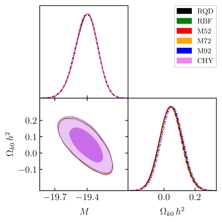
Figure 2: Contour plots for $M$ and $\Omega_{k0}h^{2}$ using different GP kernels.

Datasets	RBF	CHY	RQD	M52	M72	M92
CC	0.419	0.398	0.409	0.384	0.401	0.408
CC+BAO	0.403	0.401	0.402	0.397	0.400	0.401
SN	0.311	0.310	0.310	0.305	0.308	0.309

Table 2: Reduced $\chi^{2}$ obtained with different data sets for the following kernels. The minimum values are highlighted in bold

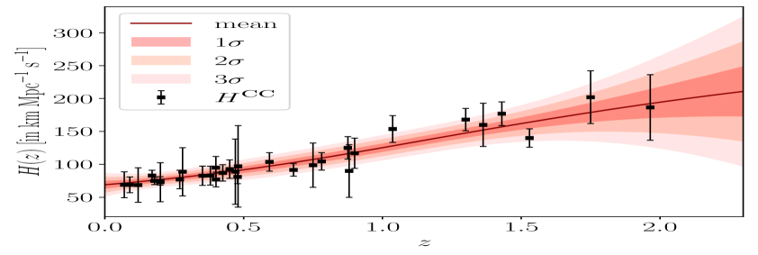
(a) Reconstructed $H(z)$

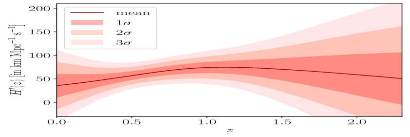
(b) Reconstructed $H^{\prime}(z)$

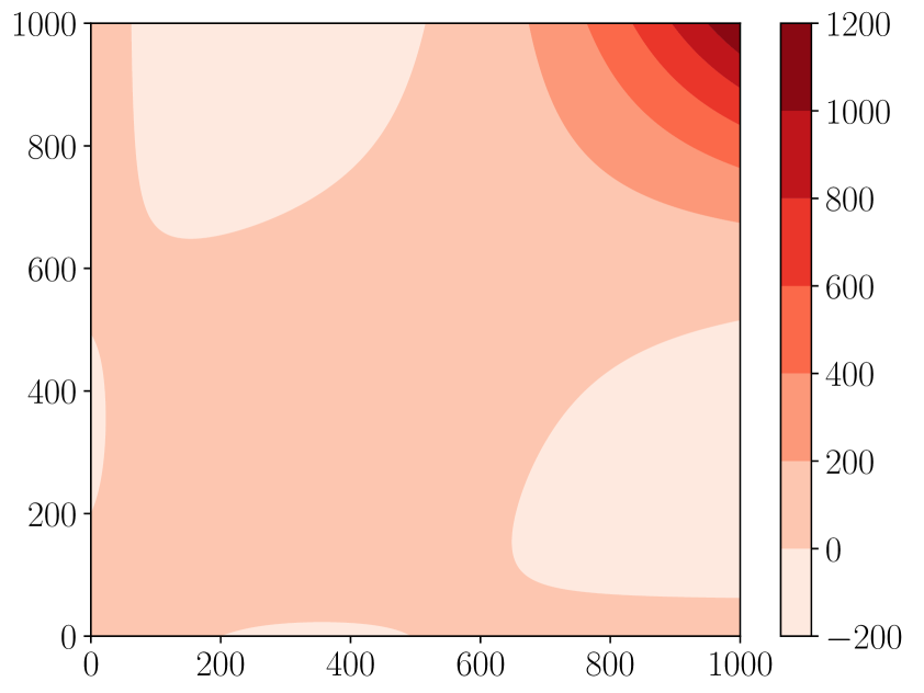
(c) cov[$H(z_{i})$, $H(z_{j})$]

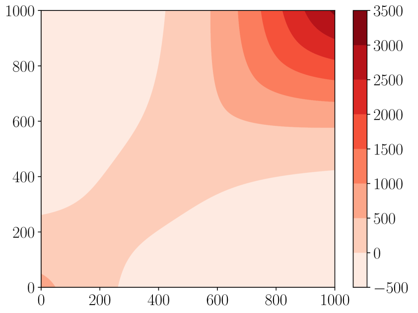
(d) cov[$H^{\prime}(z_{i})$, $H^{\prime}(z_{j})$]

(e) cov[$H(z_{i})$, $H^{\prime}(z_{j})$]

Figure 3: Reconstructed functions (a) $H(z)$, (b) $H^{\prime}(z)$ [in units of km Mpc^-1 s^-1] along with their $1\sigma$, $2\sigma$ and $3\sigma$ uncertainties using CC Hubble data set. Plots (c), (d) and (e) show the respective covariances between the predicted functions at different test redshifts.

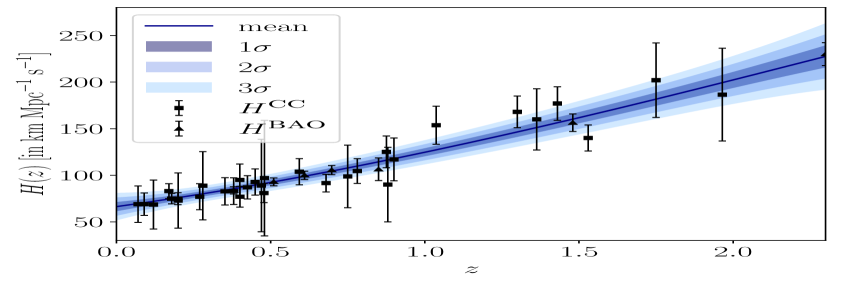
(a) Reconstructed $H(z)$

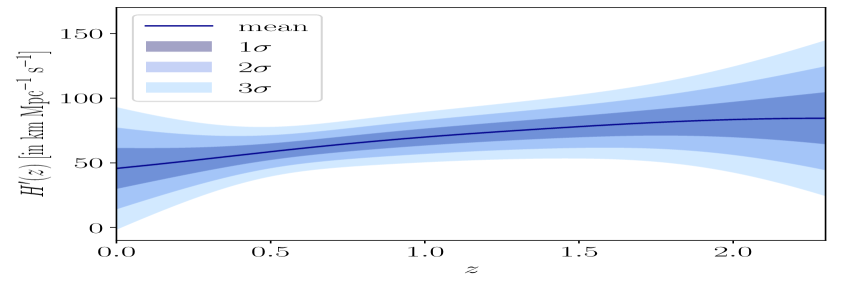
(b) Reconstructed $H^{\prime}(z)$

(c) cov[$H(z_{i})$, $H(z_{j})$]

(d) cov[$H^{\prime}(z_{i})$, $H^{\prime}(z_{j})$]

(e) cov[$H(z_{i})$, $H^{\prime}(z_{j})$]

Figure 4: Reconstructed functions (a) $H(z)$, (b) $H^{\prime}(z)$ [in units of km Mpc^-1 s^-1] along with their $1\sigma$, $2\sigma$ and $3\sigma$ confidence levels using CC+BAO Hubble data set. Plots (c), (d) and (e) show the respective covariances between the predicted functions at different test redshifts.

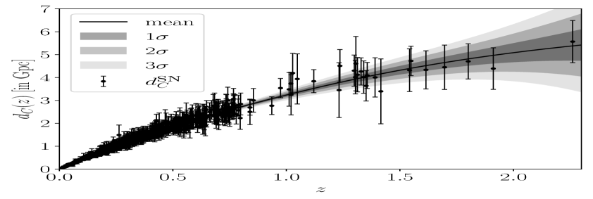
(a) Reconstructed $d_{C}(z)$

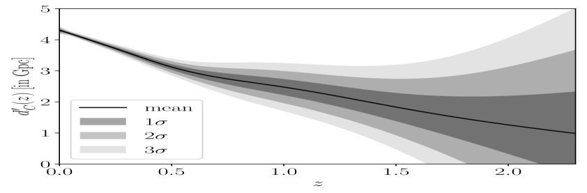
(b) Reconstructed $d_{C}^{\prime}(z)$

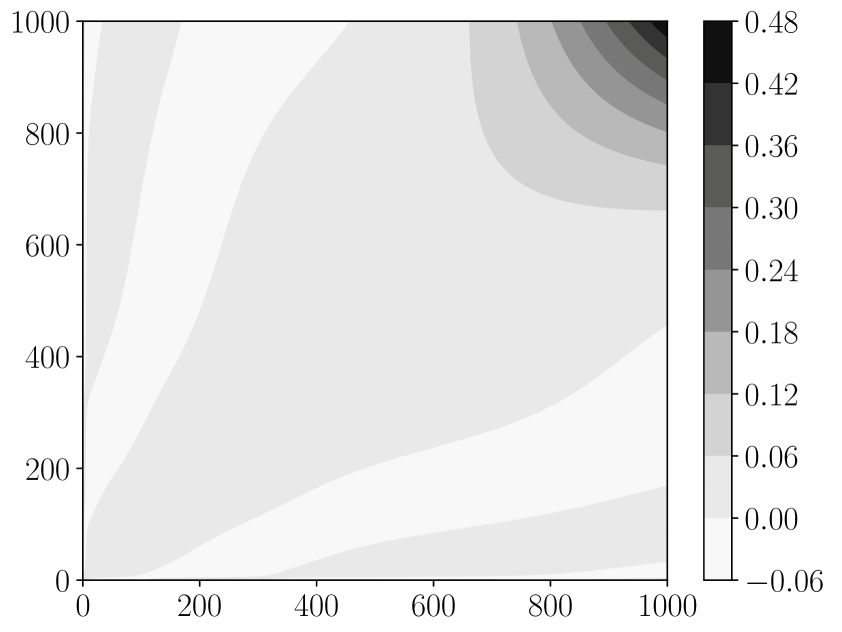
(c) cov[$d_{C}(z_{i})$, $d_{C}(z_{j})$]

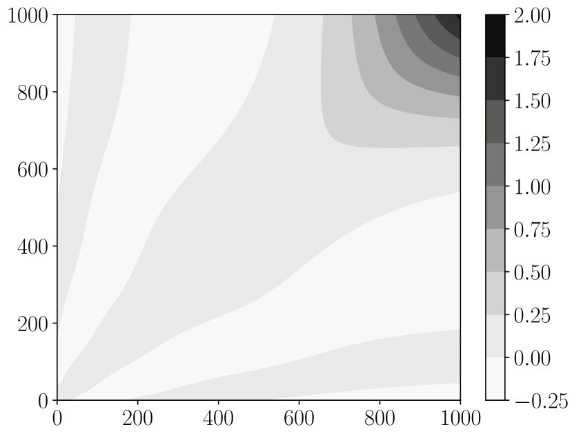
(d) cov[$d_{C}^{\prime}(z_{i})$, $d_{C}^{\prime}(z_{j})$]

(e) cov[$d_{C}(z_{i})$, $d_{C}^{\prime}(z_{j})$]

Figure 5: Reconstructed functions (a) $d_{C}(z)$, (b) $d_{C}^{\prime}(z)$ [in units of Gpc] along with their $1\sigma$, $2\sigma$ and $3\sigma$ confidence intervals using Pantheon+ SN Ia data set. Plots (c), (d) and (e) show the respective covariances between the predicted functions at different test redshifts.

To begin with, we undertake a Gaussian process reconstruction of the Hubble parameter $H(z)$ and its derivative $H^{\prime}(z)$ from the recent 32 CC and combined 32 CC + 8 BAO data. The CC Hubble data depend on the differential ages of galaxies and do not assume any particular cosmological model [11, 12, 13, 14, 15, 16, 17, 18]. We also take into account the systematic uncertainties reported in Moresco et al. [19]. Again, the BAO measurements [20, 21, 22, 23, 24, 25, 26, 27] make use of a fiducial radius of the comoving sound horizon at drag epoch, $r_{d}^{\text{fid}}$, which depend on the underlying cosmology. We adopt a full marginalization over the GP hyperparameter space setting $r_{d}$ for the BAO data as an additional free parameter to obtain a model-independent Hubble data set from CC and the calibrated BAO.

We adopt a Bayesian Markov chain Monte Carlo (MCMC) analysis using the emcee [28], assuming flat priors on the kernel hyperparameters. The two dimensional confidence contours showing the uncertainties along with the one dimensional marginalized posterior probability distributions are shown in Fig. 1 for CC (left panel) and combined CC+BAO (middle panel) $H(z)$ reconstructions with GetDist [29].

From a Bayesian perspective, one should compute the predictions from full distribution of the hyperparameters, to take into account their correlations and uncertainties. In a very recent work by the present authors [30], $10^{4}$ random realizations were obtained from the full distribution of hyperparameters. This exercise was undertaken for four kernels, to investigate if the different covariance functions lead to significant changes in the final results. However, no appreciable differences was found regardless of the kernel choice. Another effort was carried out in [31] with similar conclusion.

It is expedient to abandon the assumption of a Dirac delta distribution for the hyperparameters and propagate their non-zero uncertainties to the reconstructed function. But, this entire procedure becomes computationally expensive. Besides, in the case of constant prior mean, the likelihood is almost sharply peaked, so the best-fit result becomes a good approximation. So, we compute the best-fit values of the hyperparameters to determine the predictions from our GP model.

To reconstruct the comoving distance $d_{C}(z)$, its derivative and the corresponding uncertainties, we consider the 1701 apparent magnitudes from Pantheon+ compilation of SNIa [32]. We have removed those SN data that are contained in the host galaxies of SH0ES [33, 34], in order to obtain results independent of them. The observed 1624 apparent magnitudes $\tilde{m}$ for each SN Ia lightcurve as measured on Earth depends on heliocentric $z_{\text{hel}}$ and Hubble diagram $z_{\text{hd}}$ redshifts. We can rewrite the expression the apparent magnitudes in absence of peculiar motions, only in terms of the redshift $z_{\text{hd}}$ as,

$$m(z_{\text{hd}})=\tilde{m}(z_{\text{hel}},\,z_{\text{hd}})-5\,\log_{10}\left(\frac{1+z_{\text{hel}}}{1+z_{\text{hd}}}\right)=M+25+5\,\log_{10}\left[\frac{d_{L}(z_{\text{hd}})}{1\,\text{Mpc}}\right],$$ (4.5)

where $M$ is peak absolute magnitude of the supernovae.

Following a similar prescription by Dinda [35], we generate the function values $m(z)$, $m^{\prime}(z)$ and their corresponding uncertainties at the CC redshifts employing another GP. To scale down the drastic variance in the density of data with redshift the reconstruction is carried out in $\ln(z)$. With these reconstructed $m(z)$ and $m^{\prime}(z)$, we obtain the model-independent constraints on $M$ by minimizing the $\chi^{2}$ function,

$$\chi^{2}={(H^{\text{CC}}-H^{\text{SN}})}^{\text{T}}\cdot{{{{\Sigma}}}}^{-1}(H^{\text{CC}}-H^{\text{SN}})\,,$$ (4.6)

considering a uniform prior for $M\,\in\,\left[-21,-18\right]$ and $\Omega_{k0}h^{2}\,\in\,[-0.5,1]$ with $h=\frac{H_{0}}{100\,\text{km Mpc${}^{-1}$ s${}^{-1}$}}$ as the reduced, dimensionless, Hubble constant. Here, $H^{\text{CC}}$ are the CC $H(z)$ measurements, $H^{\text{SN}}$ is the Hubble parameter derived from the SN data, and ${{\Sigma}}\equiv\Sigma^{\text{CC}}+\Sigma^{\text{SN}}$ is the total covariance matrix. Therefore $H^{\text{SN}}$ is given by,

$$H^{\text{SN}}=\left\{\frac{(1+z)^{2}\left[c^{2}\,(1+z)^{2}+\Omega_{k0}\,H_{0}^{2}\,d_{L}^{2}\right]}{\left[(1+z)d_{L}^{\prime}-d_{L}\right]^{2}}\right\}^{\frac{1}{2}},$$ (4.7)

where $d_{L}$ and $d_{L}^{\prime}$ are the luminosity distances and its derivatives that can be computed from the reconstructed $m$ and $m^{\prime}$ values as,

$$d_{L}(z) =10^{\frac{1}{5}\left(m-M-25\right)},$$ (4.8)

$$d_{L}^{\prime}(z) =m^{\prime}\,\frac{\log{(10)}}{5}\,10^{\frac{m-M-25}{5}}.$$ (4.9)

Plots for the marginalized constraints on $M$, obtained via MCMC analysis, is shown in Fig. 2. Note that, although these constraints are model-independent they implicitly assume the validity of the cosmic distance duality relation.

The best fit values and 1$\sigma$ uncertainties for the parameters $M$, $\Omega_{k0}\,h^{2}$ for the CC calibrated SN data, and $r_{d}$ from the CC calibrated BAO data is given in Table 1.

With the respective constraints on $M$, we can generate the comoving distance data using Eq. (2.5) in Eq. (4.8). Finally, we can carry out a GP reconstruction of the functions $d_{C}(z)$, $d_{C}^{\prime}(z)$ and the respective uncertainties. A triangle plot showing the marginalized posteriors of the GP hyperparameters for $d_{C}(z)$ is shown in the right panel of Fig. 1.

To determine the most suitable kernel we select the associated GP model that gives the minimum $\chi^{2}$ between the observations vs reconstructed values at the training redshifts. Table 2 gives the reduced best-fit $\chi^{2}$ obtained with different data sets for the six kernels. We also compare the effects resulting from the remaining best-fit kernel choices. We find that the Matérn $\nu=5/2$ (M52) kernel performs better in comparison to the others. As the M52 kernel has the largest posterior distribution in all situations, it indicates that the GP reconstructed functions employing the M52 kernel seems to be the closest to the real data and hence can be considered as a better model. Recently, Zhang et al [36] arrived at similar results using the ABC Rejection algorithm for kernel selection.

We show the plots for the reconstructed functions, $H(z)$, $H^{\prime}(z)$, from the CC and combined CC+BAO data sets in Figs. 3 and 4 respectively. The reconstructed profile of $d_{C}(z)$ and $d_{C}^{\prime}(z)$ from the Pantheon+ SN data is shown in Fig. 5. We also plot the correlations between the reconstructed functions and their derivatives simultaneously. All the figures above have been generated employing the Matérn 5/2 covariance function.

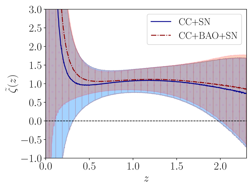
(a) RBF

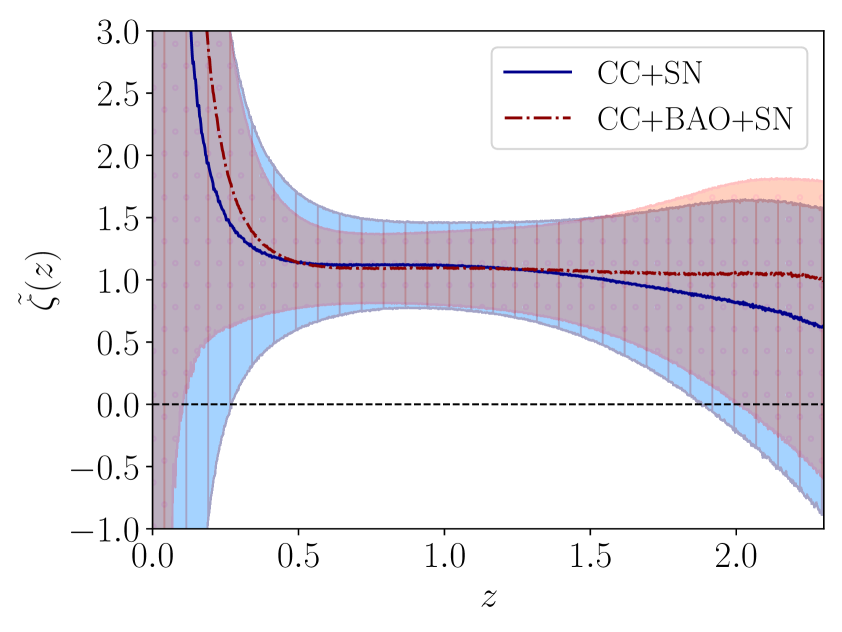
(b) CHY

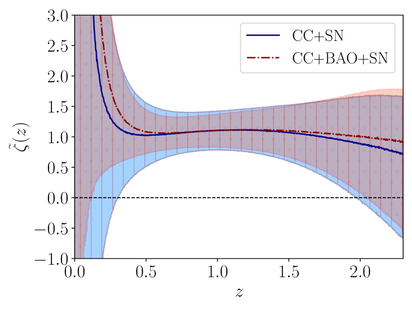
(c) RQD

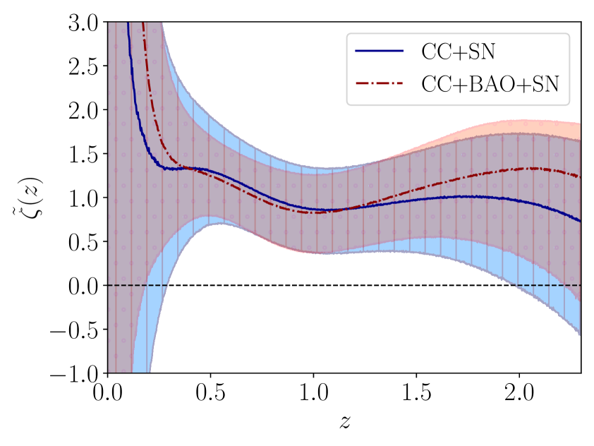
(d) M52

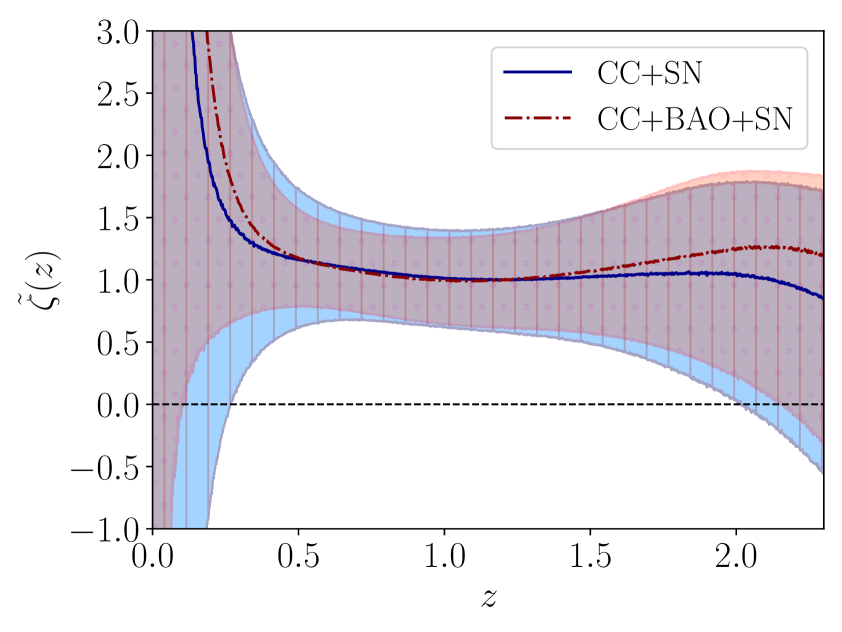
(e) M72

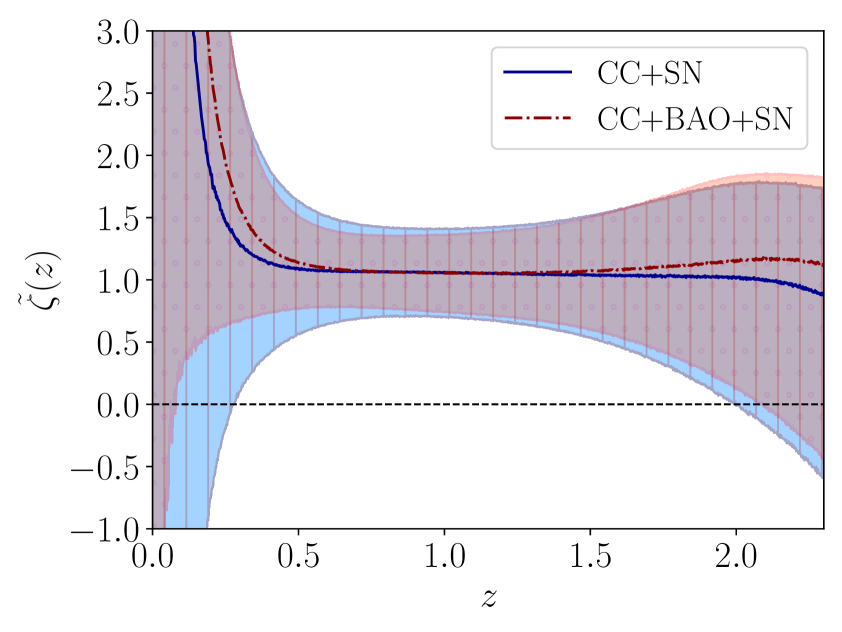
(f) M92

Figure 6: Reconstructed $\tilde{\zeta}$, after using Eq. (3.3) from CC+SN (solid lines) and CC+BAO+SN (dash-dot lines) data set combinations for different kernel choices. The shaded regions with ‘|’ and ‘$\cdot$’ hatches represent the 1$\sigma$ confidence levels for the CC+SN and CC+BAO+SN combinations respectively. $\tilde{\zeta}$ diverges when $z$ approaches zero because so does $d_{C}$.

5 Results

Finally, with the reconstructed functions $H(z)$, $H^{\prime}(z)$, $d_{C}(z)$ and $d_{C}^{\prime}(z)$, we now derive the evolution of $\zeta$, defined by Eq. (3.3) as a function of the cosmological redshift. Alternatively, we can substitute the constraints obtained on $\Omega_{k0}h^{2}$, given in Table 1, to arrive at $\Omega_{k0}H_{0}^{2}$ and directly use Eq. (3.1) to reconstruct $\zeta(z)$.

However, in equations (3.1) and (3.3), $\zeta$ has units of the Hubble factor. This is made clear by writing Eq. (3.1) and (3.3) as,

$$\zeta(z)\equiv H_{0}\left[E^{\prime}(z)-\Omega_{k0}\frac{1+z}{E(z)}\right]\geq 0$$ (5.1)

or, equivalently,

$$\zeta(z)\equiv H_{0}\left[E^{\prime}(z)-\frac{E^{2}(z)\,D^{\prime 2}(z)-1}{D^{2}(z)}\,\frac{1+z}{E(z)}\right]\geq 0.$$ (5.2)

Obviously, it is expedient to have a dimensionless representation. So, we use $\tilde{\zeta}\equiv\zeta/H_{0}$ with $H_{0}=73.3\text{ km Mpc${}^{-1}$ s${}^{-1}$}$, the central SH0ES value for the Hubble constant [33]. It deserves mention that this assumption serves the purpose of a rescaling just to make the reconstructed quantity dimensionless. So, our final results are independent of this choice.

Figure 6 shows plots of the evolution of $\tilde{\zeta}$ along with their 1$\sigma$ confidence levels for the CC+SN and CC+BAO+SN data set combinations. Here, we show the results obtained with different reconstruction kernels for comparison and better illustration. Note that the reconstructed $\tilde{\zeta}$ from Eq. (3.3) has a divergence since $d_{C}(z=0)=0$ brings a singularity at $z=0$.

We also plot for the redshift evolution of $\tilde{\zeta}$ using Eq. (3.1) along with its 1$\sigma$ confidence levels in Fig. 7 for the CC+$\Omega_{k0}H_{0}^{2}$ and CC+BAO+$\Omega_{k0}H_{0}^{2}$ combinations. We take into account the correlations between the reconstructed functions and their derivatives, and compute the uncertainties associated with $\tilde{\zeta}$ via the Monte Carlo error propagation rule.

As is apparent in these figures neither the solid nor the dashed-dot lines ever cross the horizontal axis $\tilde{\zeta}=0$.

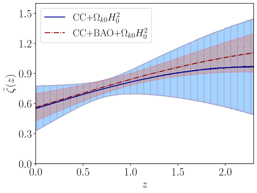
(a) RBF

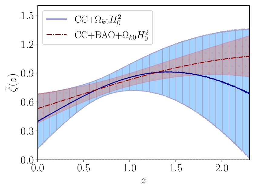
(b) CHY

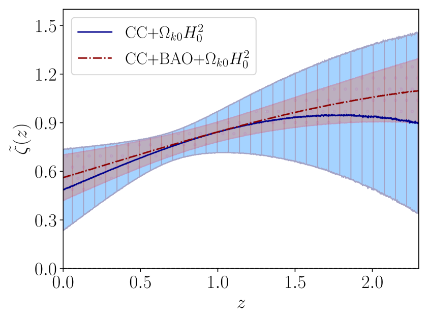
(c) RQD

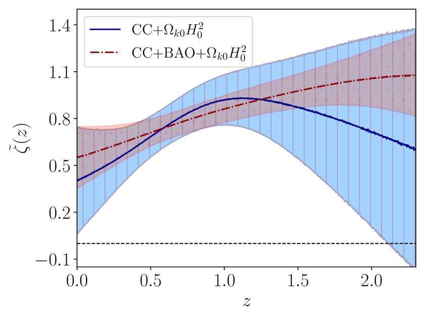
(d) M52

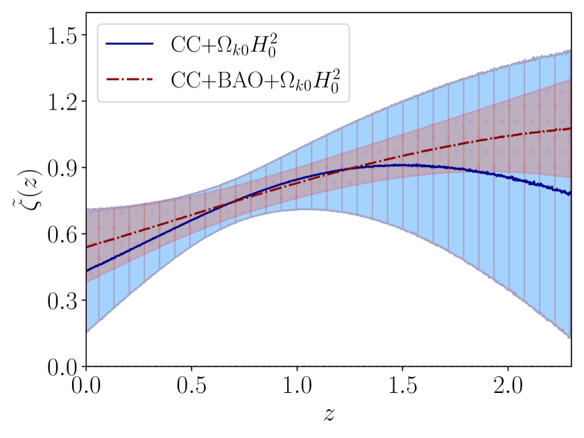
(e) M72

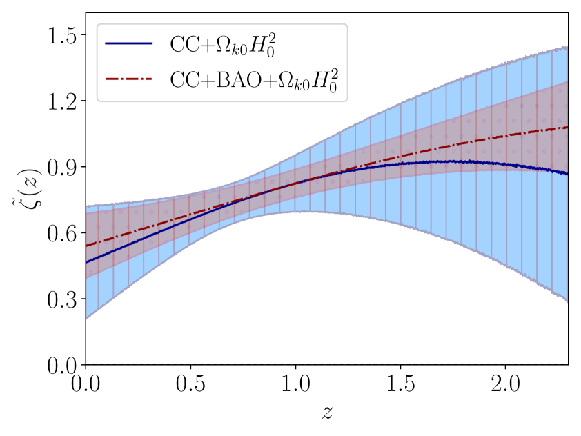
(f) M92

Figure 7: Reconstructed $\tilde{\zeta}$, derived using Eq. (3.1) from CC+$\Omega_{k0}H_{0}^{2}$ (solid lines) and CC+BAO+$\Omega_{k0}H_{0}^{2}$ (dash-dot lines) combinations for different kernel choices. The shaded regions with ‘|’ and ‘$\cdot$’ hatches represent the 1$\sigma$ confidence levels for the CC+$\Omega_{k0}H_{0}^{2}$ and CC+BAO+$\Omega_{k0}H_{0}^{2}$ combinations respectively.

Before closing this section, it is worth mentioning that our findings severely constrain universe models in which phantom dark energy dominates the expansion. In such models the expansion is super-accelerated ($\dot{H}>0$), i.e. $q<-1$. While observational data do not exclude them [37], and new proposals have been made recently [38], equation (2.1) and the fact that the data strongly suggest that $\Omega_{k0}$ is either zero or very close to it [37], it follows that it is extremely likely that $q\geq-1$ and that $\tilde{\zeta}>0$. Although the results summarized in Fig. 6 do not rule out entirely the possibility $\tilde{\zeta}<0$ in the redshift range $0<z<2$, the results summarized in Fig. 7 do. In addition, phantom models face serious difficulties from the theoretical side since, their energy density being unbounded from below, they do not appear stable either from quantum consideration [39] or even classically [40].

6 Concluding Remarks

Our study, based solely on Einstein gravity and the assumption that the Universe is homogeneous and isotropic, backs previous analysis about the question, “is the second law of thermodynamics satisfied at cosmic scales?” After making use of the history of thee Hubble function in the redshift range $0<z\leq 2$ we find the answer in the affirmative. Indeed, as Figs. 6 and 7 show, $\tilde{\zeta}$ stays positive in the said range; i.e., the inequality $1+q\geq\Omega_{k}$ is fulfilled in that interval irrespective of whether $\Omega_{k}$ is positive, negative or nil. This means that the history of the Hubble function tells us that the area of the apparent horizon does not decrease with expansion. In other words, the mentioned history is compatible with second law of thermodynamics at cosmic scales as it was suggested by quite different methods in [2] and [41]. This result is most reassuring; it would be weird that this law, being valid at terrestrial and astrophysical scales, would fail at cosmic scales. Finally, as a by product, this work strengthens our belief that the Universe was never dominated by phantom fields in the considered redshift range.

References

- [1] C. A. Egan and C.H. Lineweaver, A larger estimate of the entropy of the Universe, Astrophys. J. 710 (2010) 1825 [0909.3983v3].
- [2] M. Gonzalez-Espinoza and D. Pavón, Does the second law hold at cosmic scales?, Mon. Not. Roy. Astron. Soc. 484 (2019) 2924 [1902.06651].
- [3] C.E. Rasmussen and C.K.I. Williams Gaussian Processes for Machine Learning, The MIT Press, Cambridge (2005)
- [4] M. Seikel, C. Clarkson and M. Smith, Reconstruction of dark energy and expansion dynamics using Gaussian processes, JCAP 06 (2012) 036 [1204.2832].
- [5] A. Shafieloo, A.G. Kim and E.V. Linder, Gaussian Process Cosmography, Phys. Rev. D 85 (2012) 123530, [1204.2272].
- [6] D. Bak and S. Rey, Cosmic holography, Class. Quantum Grav. 17 (2000) L83 [hep-th/9902173].
- [7] R.-G. Cai, Z.-K. Guo and T. Yang, Null test of the cosmic curvature using and supernovae data, Phys. Rev. D 93 (2016) 043517 [1509.06283].
- [8] Y. Yang and Y. Gong, Measurement on the cosmic curvature using the Gaussian process method, Mon. Not. Roy. Astron. Soc. 504 (2021) 3092 [2007.05714].
- [9] P. Mukherjee and N. Banerjee, Constraining the curvature density parameter in cosmology, Phys. Rev. D 105 (2022) 063516 [2202.07886].
- [10] R.A. Daly et al., Improved constraints on the acceleration history of the Universe and the properties of the dark energy, Astrophys. J. 677 (2008) 1 [0710.5345].
- [11] D. Stern, R. Jimenez, L. Verde, M. Kamionkowski and S.A. Stanford, Cosmic Chronometers: Constraining the Equation of State of Dark Energy. I: Measurements, JCAP 02 (2010) 008 [0907.3149].
- [12] M. Moresco, A. Cimatti, R. Jimenez, L. Pozzetti et al., Improved constraints on the expansion rate of the universe up to from the spectroscopic evolution of cosmic chronometers, JCAP 08 (2012) 006, [1201.3609].
- [13] C. Zhang, H. Zhang, S. Yuan, T.-J. Zhang and Y.-C. Sun, Four new observational data from luminous red galaxies in the Sloan Digital Sky Survey data release seven, Res. Astron. Astrophys. 14 (2014) 1221 [1207.4541].
- [14] M. Moresco, Raising the bar: new constraints on the Hubble parameter with cosmic chronometers at z 2, Mon. Not. Roy. Astron. Soc. 450 (2015) L16 [1503.01116].
- [15] M. Moresco, L. Pozzetti, A. Cimatti, R. Jimenez, C. Maraston, L. Verde et al., A 6% measurement of the Hubble parameter at : direct evidence of the epoch of cosmic re-acceleration, JCAP 05 (2016) 014 [1601.01701].
- [16] A.L. Ratsimbazafy, S.I. Loubser, S.M. Crawford, C.M. Cress, B.A. Bassett, R.C. Nichol et al., Age-dating Luminous Red Galaxies observed with the Southern African Large Telescope, Mon. Not. Roy. Astron. Soc. 467 (2017) 3239 [1702.00418].
- [17] N. Borghi, M. Moresco and A. Cimatti, Toward a Better Understanding of Cosmic Chronometers: A New Measurement of H(z) at z 0.7, Astrophys. J. Lett. 928 (2022) L4 [2110.04304].
- [18] K. Jiao, N. Borghi, M. Moresco and T.-J. Zhang, New Observational H(z) Data from Full-spectrum Fitting of Cosmic Chronometers in the LEGA-C Survey, Astrophys. J. Suppl. 265 (2023) 48 [2205.05701].
- [19] M. Moresco, R. Jimenez, L. Verde, A. Cimatti and L. Pozzetti, Setting the Stage for Cosmic Chronometers. II. Impact of Stellar Population Synthesis Models Systematics and Full Covariance Matrix, Astrophys. J. 898 (2020) 82 [2003.07362].
- [20] S. Alam et al. (BOSS Collaboration), The clustering of galaxies in the completed SDSS-III Baryon Oscillation Spectroscopic Survey: cosmological analysis of the DR12 galaxy sample, Mon. Not. Roy. Astron. Soc. 470 (2017) 2617 [1607.03155].
- [21] J.E. Bautista et al., The Completed SDSS-IV extended Baryon Oscillation Spectroscopic Survey: measurement of the BAO and growth rate of structure of the luminous red galaxy sample from the anisotropic correlation function between redshifts 0.6 and 1, Mon. Not. Roy. Astron. Soc. 500 (2020) 736 [2007.08993].
- [22] H. Gil-Marin et al., The Completed SDSS-IV extended Baryon Oscillation Spectroscopic Survey: measurement of the BAO and growth rate of structure of the luminous red galaxy sample from the anisotropic power spectrum between redshifts 0.6 and 1.0, Mon. Not. Roy. Astron. Soc. 498 (2020) 2492 [2007.08994].
- [23] R. Neveux et al., The completed SDSS-IV extended Baryon Oscillation Spectroscopic Survey: BAO and RSD measurements from the anisotropic power spectrum of the quasar sample between redshift 0.8 and 2.2, Mon. Not. Roy. Astron. Soc. 499 (2020) 210 [2007.08999].
- [24] J. Hou et al., The Completed SDSS-IV extended Baryon Oscillation Spectroscopic Survey: BAO and RSD measurements from anisotropic clustering analysis of the Quasar Sample in configuration space between redshift 0.8 and 2.2, Mon. Not. Roy. Astron. Soc. 500 (2020) 1201 [2007.08998].
- [25] A. Tamone et al., The Completed SDSS-IV extended Baryon Oscillation Spectroscopic Survey: Growth rate of structure measurement from anisotropic clustering analysis in configuration space between redshift 0.6 and 1.1 for the Emission Line Galaxy sample, Mon. Not. Roy. Astron. Soc. 499 (2020) 5527 [2007.09009].
- [26] A. de Mattia et al., The Completed SDSS-IV extended Baryon Oscillation Spectroscopic Survey: measurement of the BAO and growth rate of structure of the emission line galaxy sample from the anisotropic power spectrum between redshift 0.6 and 1.1, Mon. Not. Roy. Astron. Soc. 501 (2021) 5616, [2007.09008].
- [27] J.E. Bautista et al., Measurement of baryon acoustic oscillation correlations at with SDSS DR12 Ly-Forests, Astron. Astrophys. 603 (2017) A12 [1702.00176].
- [28] D. Foreman-Mackey, D.W. Hogg, D. Lang and J. Goodman, emcee: The MCMC Hammer, Publ. Astron. Soc. Pac. 125 (2013) 306 [1202.3665].
- [29] A. Lewis, GetDist: a Python package for analysing Monte Carlo samples, 1910.13970.
- [30] N. Banerjee, P. Mukherjee and D. Pavón, Spatial curvature and thermodynamics, Mon. Not. Roy. Astron. Soc. 521 (2023) 5473 [2301.09823].
- [31] A. Favale, A. Gómez-Valent and M. Migliaccio, Cosmic chronometers to calibrate the ladders and measure the curvature of the Universe. A model-independent study, Mon. Not. Roy. Astron. Soc. 523 (2023) 3406 [2301.09591].
- [32] D. Scolnic et al., The Pantheon+ Analysis: The Full Data Set and Light-curve Release, Astrophys. J. 938 (2022) 113 [2112.03863].
- [33] A.G. Riess et al., A Comprehensive Measurement of the Local Value of the Hubble Constant with 1 km s-1 Mpc-1 Uncertainty from the Hubble Space Telescope and the SH0ES Team, Astrophys. J. Lett. 934 (2022) L7 [2112.04510].
- [34] D. Brout et al., The Pantheon+ Analysis: Cosmological Constraints, Astrophys. J. 938 (2022) 110 [2202.04077].
- [35] B.R. Dinda, Minimal model dependent constraints on cosmological nuisance parameters and cosmic curvature from combinations of cosmological data, 2209.14639.
- [36] H. Zhang, Y.-C. Wang, T.-J. Zhang and T.-t. Zhang, Kernel Selection for Gaussian Process in Cosmology: With Approximate Bayesian Computation Rejection and Nested Sampling, Astrophys. J. Suppl. 266 (2023) 27 [2304.03911].
- [37] Planck collaboration: N. Aghanim et al. Planck2018 results.VI. Cosmological parameters, Astron. Astrophys. 641 (2020) A6 [1807.06209].
- [38] M. Cruz, S. Lepe and G.E. Soto, Phantom cosmologies from QCD ghost dark energy, Phys. Rev. D 106 (2022) 103508 [2209.04584].
- [39] J.M. Cline, S. Jeon and J.D. Moore, The phantom menaced: Constraints on low-energy effective ghosts, Phys. Rev. D 70 (2004) 043543 [0311312].
- [40] M.P. Dabrowski, Puzzles of the dark energy in the universe - phantom, Eur. J. Phys. C 36 (2015) 065017 [1411.2827].
- [41] J.P. Mimoso and D. Pavón, Fluctuations of the flux of energy on the apparent horizon, Phys. Rev. D 97 (2018) 103537 [1805.02894].