A rigorous model reduction for the anisotropic-scattering transport process

Abstract

In this letter, we propose a reduced-order model to bridge the particle transport mechanics and the macroscopic fluid dynamics in the highly scattered regime. A rigorous mathematical derivation and a concise physical interpretation are presented for an anisotropic-scattering transport process with arbitrary order of scattering kernel. The prediction of the theoretical model perfectly agrees with the numerical experiments. A clear picture of the diffusion physics is revealed for the neutral particle transport in the asymptotic optically thick regime.

I Introduction

In the statistic physics of particle transport, one objective is to construct a solid mathematical basis and axiomatize the multiscale hierarchy modeling of the physics of particle transport [1]. In 1872, Boltzmann devised the Boltzmann transport equation, in which the positions and momenta of particles are characterized by the probability distribution function. The Boltzmann equation bridges the microscopic Lagrangian mechanics to the mesoscopic kinetic mechanics and reduces the degree of freedom of the system to seven dimensions, i.e., the physical space, the velocity space, and time. The asymptotic theories developed by Hilbert, Chapman, and Cowling in the 1910s provide a framework for analyzing the structure of the probability distribution function, based on which a low-dimensional model of the macroscopic hydrodynamic system is derived in the asymptotic limit of the continuum regime [2], and conscious progress has been made during the past decades [3, 4]. The asymptotic analysis reveals that the physics of momentum and energy diffusion is the particle momentum and energy exchange, and the closure modeling of the distribution function is based on a balance of the particle streaming and the particle collision processes. The macroscopic viscous and diffusion coefficients are precisely related to the microscopic particle interaction, including the potential and the cross-section. In the applications of aerodynamics and high-energy-density engineering, The asymptotic low-order models contribute to the development of efficient numerical methods for the simulation of the rarefied gas dynamics and the transport of plasma and neutral particles. For the transport process of neutral particles, Larsen et al. developed the asymptotic low-order diffusion models in the optically thick regime with an isotropic scattering [5, 6]. The rigorous mathematical analysis for the anisotropic-scattering transport process is still open. In this letter, we give a rigorous mathematical derivation of the asymptotic model for the general anisotropic-scattering transport process. The mathematical derivation, physical interpretation, and numerical experiments are presented.

II Mathematical derivation

We analyze the radiation transport equation for the anisotropic-scattering photon transport grey model here, while the derivation and conclusions are also appropriate for other neutral particles, such as neutrons. Considering a pure scattering medium and leaving out the other source terms, the grey thermal radiation transport equation can be written in the following scaled form,

$$\left\{\begin{aligned} &\frac{\partial I}{\partial t}+\frac{c}{\varepsilon}\vec{\Omega}\cdot\nabla I=\frac{c\sigma_{s}}{\varepsilon^{2}}\left(S-I\right),\\ &S=\int p\left(\vec{\Omega}^{\prime}\rightarrow\vec{\Omega}\right)I\left(\vec{\Omega}^{\prime}\right)d\vec{\Omega}^{\prime}.\end{aligned}\right.$$ (1)

Here $I$ is the radiation intensity, $c$ is the speed of light, $\sigma_{s}$ is the scattering coefficient, $S$ is the scattering source, $\vec{\Omega}$ and $\vec{\Omega}^{\prime}$ are the outgoing and incoming direction angular variable, $p\left(\vec{\Omega}^{\prime}\rightarrow\vec{\Omega}\right)$ is the scattering phase function, $\varepsilon$ is the Knudsen number, i.e., the ratio between the local mean free path and the characteristic length. The scattering kernel $p\left(\vec{\Omega}^{\prime}\rightarrow\vec{\Omega}\right)$ can be expanded in the Legendre polynomial space as

$$p\left(\vec{\Omega}^{\prime}\rightarrow\vec{\Omega}\right)=\sum_{l=0}^{L}C_{l}P_{l}\left(\vec{\Omega}^{\prime}\cdot\vec{\Omega}\right),$$ (2)

where $C_{l}$ is the coefficient of the $l$-order Legendre basis.

Lemma II.1.

The scattering source $S$ is related to the moments of $I$ by

$$S=\sum_{l=0}^{L}C_{l}^{\ast}\sum_{i_{1}i_{2}\cdots i_{l}}\left(\Omega_{i_{1}i_{2}\cdots i_{l}}^{\left(l\right)}J_{i_{1}i_{2}\cdots i_{l}}^{\left(l\right)}\right)$$ (3)

where $\Omega_{i_{1}i_{2}\cdots i_{l}}^{\left(l\right)}=\Omega_{i_{1}}\Omega_{i_{2}}\cdots\Omega_{i_{l}}$, the index $i_{k}\in\{x,y,z\}$ with the corresponding direction cosine $\Omega_{i_{k}}\in\{\mu,\xi,\zeta\}$ and $k\in\left[0,l\right]$. $J^{\left(l\right)}$ is the $l$th-order moments of $I$, and $J_{i_{1}i_{2}\cdots i_{l}}^{\left(l\right)}$ is the $\{i_{1}i_{2}\cdots i_{l}\}$ component of $J^{(l)}$, $\sum_{i_{1}i_{2}\cdots i_{l}}$ means the summation for all possible combinations of index $\{i_{1}i_{2}\cdots i_{l}\}$.

Proof.

The scattering phase function (2) can be further written as the sum of a finite series of polynomials:

$$p\left(\vec{\Omega}^{\prime}\rightarrow\vec{\Omega}\right)=\sum_{l=0}^{L}C_{l}^{\ast}\left(\vec{\Omega}^{\prime}\cdot\vec{\Omega}\right)^{l}=\sum_{l=0}^{L}C_{l}^{\ast}\left(\cos\theta\right)^{l}.$$ (4)

Here $C_{l}^{\ast}$ are the corresponding coefficients of $l$th polynomial $\left(\vec{\Omega}^{\prime}\cdot\vec{\Omega}\right)^{l}$, $\theta$ is the scattering angle between $\vec{\Omega}^{\prime}$ and $\vec{\Omega}$. Thus, the scattering source $S$ can be written as:

$$S=\sum_{l=0}^{L}C_{l}^{\ast}\left(\int\left(\vec{\Omega}^{\prime}\cdot\vec{\Omega}\right)^{l}I\left(\vec{\Omega}^{\prime}\right)d\vec{\Omega}^{\prime}\right).$$ (5)

In three-dimensional Cartesian velocity space, we have

$$\left(\vec{\Omega}^{\prime}\cdot\vec{\Omega}\right)^{l}= \left(\mu\mu^{\prime}+\xi\xi^{\prime}+\zeta\zeta^{\prime}\right)^{l}=\sum_{i_{1}i_{2}\cdots i_{l}}\Omega_{i_{1}i_{2}\cdots i_{l}}^{\left(l\right)}\Omega_{i_{1}i_{2}\cdots i_{l}}^{\prime\left(l\right)},$$ (6)

with $\Omega_{i_{1}i_{2}\cdots i_{l}}^{\prime\left(l\right)}=\Omega_{i_{1}}^{\prime}\Omega_{i_{2}}^{\prime}\cdots\Omega_{i_{l}}^{\prime}$ and $\Omega_{i_{k}}^{\prime}\in\{\mu^{\prime},\xi^{\prime},\zeta^{\prime}\}$. Therefore, the angular integration term in (5) for arbitrary $l$ is:

$$\int\left(\vec{\Omega}^{\prime}\cdot\vec{\Omega}\right)^{l}I\left(\vec{\Omega}^{\prime}\right)d\vec{\Omega}^{\prime}=\sum_{i_{1}i_{2}\cdots i_{l}}\left(\Omega_{i_{1}i_{2}\cdots i_{l}}^{\left(l\right)}J_{i_{1}i_{2}\cdots i_{l}}^{\left(l\right)}\right),$$ (7)

with $J_{i_{1}i_{2}\cdots i_{l}}^{\left(l\right)}=\int\Omega_{i_{1}i_{2}\cdots i_{l}}^{\prime\left(l\right)}I\left(\vec{\Omega}^{\prime}\right)d\vec{\Omega}^{\prime}$. Substituting (7) into equation (5) gives equation (3). ∎

Proposition II.1.1.

Define $S^{\left(q\right)}$ as the $q$th-order moments of $S$. The odd-order moments $S^{(n=odd)}$ is only related to $J^{(l=odd)}$, and the even-order moments $S^{(m=even)}$ is only related to $J^{(l=even)}$.

Proof.

Based on Lemma II.1, the components of $S^{(q)}$ is given by:

$$S_{i_{1}i_{2}\cdots i_{q}}^{\left(q\right)}=\sum_{l=0}^{L}C_{l}^{\ast}\sum_{i_{1}i_{2}\cdots i_{l}}\left(\left<\Omega_{i_{1}i_{2}\cdots i_{q}}^{\left(q\right)}\Omega_{i_{1}i_{2}\cdots i_{l}}^{\left(l\right)}\right>J_{i_{1}i_{2}\cdots i_{l}}^{\left(l\right)}\right),$$ (8)

where $\left<\cdot\right>$ means angular integration. The angular integration term has the property

$$\left<\mu^{r}\xi^{s}\zeta^{t}\right>\left\{\begin{aligned} &\neq 0,\quad r,s,t\text{ are even numbers},\\ &=0,\quad r,s,t\text{ has odd number}.\end{aligned}\right.$$ (9)

Therefore, we have

$$\left<\Omega_{i_{1}i_{2}\cdots i_{q}}^{\left(q\right)}\Omega_{i_{1}i_{2}\cdots i_{l}}^{\left(l\right)}\right>=0,\text{ for }q+l=odd.$$ (10)

Hence, $S^{\left(n=odd\right)}$ is only related to $J^{\left(l=odd\right)}$, and $S^{\left(m=even\right)}$ is only related to $J^{\left(l=even\right)}$,

$$\footnotesize\left\{\begin{aligned} &S_{i_{1}i_{2}\cdots i_{n}}^{\left(n=odd\right)}=\sum_{l=odd}^{L}C_{l}^{\ast}\sum_{i_{1}i_{2}\cdots i_{l}}^{l=odd}\left(\left<\Omega_{i_{1}i_{2}\cdots i_{n}}^{\left(n\right)}\Omega_{i_{1}i_{2}\cdots i_{l}}^{\left(l\right)}\right>J_{i_{1}i_{2}\cdots i_{l}}^{\left(l\right)}\right),\\ &S_{i_{1}i_{2}\cdots i_{m}}^{\left(m=even\right)}=\sum_{l=even}^{L}C_{l}^{\ast}\sum_{i_{1}i_{2}\cdots i_{l}}^{l=even}\left(\left<\Omega_{i_{1}i_{2}\cdots i_{m}}^{\left(m\right)}\Omega_{i_{1}i_{2}\cdots i_{l}}^{\left(l\right)}\right>J_{i_{1}i_{2}\cdots i_{l}}^{\left(l\right)}\right).\end{aligned}\right.$$ (11)

∎

Lemma II.2.

The arbitrary even-order angular moments satisfy $J_{i_{1}i_{2}\cdots i_{l}}^{\left(l=even\right)}=\frac{\left<\Omega_{i_{1}i_{2}\cdots i_{l}}^{\left(l\right)}\right>}{\left<\Omega^{\left(0\right)}\right>}\rho$.

Proof.

The zeroth moments of scattering source $S$ is

$$S^{(0)}= \int_{\vec{\Omega}^{\prime}}\left(\int_{\vec{\Omega}}p\left(\vec{\Omega}^{\prime}\rightarrow\vec{\Omega}\right)d\vec{\Omega}\right)I\left(\vec{\Omega}^{\prime}\right)d\vec{\Omega}^{\prime}=\rho,$$ (12)

namely, the anisotropic scattering conserves the radiation energy. Based on the normalization condition of the phase function, we have

$$\int_{\vec{\Omega}^{\prime}}p\left(\vec{\Omega}^{\prime}\rightarrow\vec{\Omega}\right)d\vec{\Omega}^{\prime}=\sum_{l}^{L}C_{l}^{\ast}\int_{\vec{\Omega}^{\prime}}\left(\vec{\Omega}^{\prime}\cdot\vec{\Omega}\right)^{l}d\vec{\Omega}^{\prime}$$ (13)

$$=\sum_{l=even}^{L}C_{l}^{\ast}\sum_{i_{1}i_{2}\cdots i_{l}}^{l=even}\left(\left<\Omega_{i_{1}i_{2}\cdots i_{l}}^{\prime\left(l\right)}\right>\Omega_{i_{1}i_{2}\cdots i_{l}}^{\left(l\right)}\right)=1.$$

Taking angular integration to equation (13), we have

$$\sum_{l=even}^{L}C_{l}^{\ast}\sum_{i_{1}i_{2}\cdots i_{l}}^{l=even}\left(\left<\Omega_{i_{1}i_{2}\cdots i_{l}}^{\prime\left(l\right)}\right>\left<\Omega_{i_{1}i_{2}\cdots i_{l}}^{\left(l\right)}\right>\right)=\left<\Omega^{\left(0\right)}\right>,$$ (14)

which gives

$$\sum_{l=even}^{L}C_{l}^{\ast}\sum_{i_{1}\cdots i_{l}}^{l=even}\left(\left<\Omega_{i_{1}\cdots i_{l}}^{\left(l\right)}\right>\frac{\left<\Omega_{i_{1}\cdots i_{l}}^{\left(l\right)}\right>}{\left<\Omega^{\left(0\right)}\right>}\right)=1.$$ (15)

Base on Proposition II.1.1 and equation (12), we have

$$\rho=S^{(0)}=\sum_{l=even}^{L}C_{l}^{\ast}\sum_{i_{1}i_{2}\cdots i_{l}}^{l=even}\left(\left<\Omega_{i_{1}i_{2}\cdots i_{l}}^{\left(l\right)}\right>J_{i_{1}i_{2}\cdots i_{l}}^{\left(l\right)}\right),$$ (16)

which leads to

$$\sum_{l=even}^{L}C_{l}^{\ast}\sum_{i_{1}i_{2}\cdots i_{l}}^{l=even}\left(\left<\Omega_{i_{1}i_{2}\cdots i_{l}}^{\left(l\right)}\right>\frac{J_{i_{1}i_{2}\cdots i_{l}}^{\left(l\right)}}{\rho}\right)=1.$$ (17)

Thus, equations (15) and (17) gives

$$J_{i_{1}i_{2}\cdots i_{l}}^{\left(l=even\right)}=\frac{\left<\Omega_{i_{1}i_{2}\cdots i_{l}}^{\left(l\right)}\right>}{\left<\Omega^{\left(0\right)}\right>}\rho.$$ (18)

∎

Corollary II.2.1.

If the scattering kernel $p\left(\vec{\Omega}^{\prime}\rightarrow\vec{\Omega}\right)$ contains only even-order terms, the scattering process preserves the isotropic distribution of photons.

Proof.

If the scattering kernel (2) contains only even-order terms, the scattering source $S$ satisfies

$$S= \sum_{l=even}^{L}C_{l}^{\ast}\sum_{i_{1}i_{2}\cdots i_{l}}\left(\Omega_{i_{1}i_{2}\cdots i_{l}}^{\left(l\right)}J_{i_{1}i_{2}\cdots i_{l}}^{\left(l\right)}\right)$$ (19)

$$= \frac{\rho}{\left<\Omega^{\left(0\right)}\right>}\sum_{l=even}^{L}C_{l}^{\ast}\sum_{i_{1}i_{2}\cdots i_{l}}\left(\Omega_{i_{1}i_{2}\cdots i_{l}}^{\left(l\right)}\left<\Omega_{i_{1}i_{2}\cdots i_{l}}^{\left(l\right)}\right>\right).$$

The normalization property (13) states that $S={\rho}/{\left<\Omega^{\left(0\right)}\right>}$, which shows that the scattering process preserves the isotropic distribution of photons. ∎

Lemma II.1, Proposition II.1.1, Lemma II.2, and Corollary II.2.1 hold for arbitrary order $L$ of collision kernel (2) and all flow regimes. In the following, we close the energy flux $J^{\left(1\right)}$ in the optically thick regime. According to the asymptotic theory [2], the radiant intensity can be formally expanded as

$$I=S-\varepsilon\frac{1}{\sigma_{s}}\vec{\Omega}\cdot\nabla S+O(\varepsilon^{2}).$$ (20)

According to Proposition II.1.1, the radiant energy flux $J^{\left(1\right)}$ has the form

$$J^{\left(1\right)}= S^{\left(1\right)}-\varepsilon\frac{1}{\sigma_{s}}\nabla\cdot S^{\left(2\right)}+O(\varepsilon^{2})$$ (21)

$$= \sum_{l=odd}^{L}C_{l}^{\ast}\sum_{i_{1}i_{2}\cdots i_{l}}^{l=odd}\left(\left<\Omega^{\left(1\right)}\Omega_{i_{1}i_{2}\cdots i_{l}}^{\left(l\right)}\right>J_{i_{1}i_{2}\cdots i_{l}}^{\left(l\right)}\right)$$

$$-\varepsilon\frac{1}{\sigma_{s}}\nabla\cdot\sum_{l=even}^{L}C_{l}^{\ast}\sum_{i_{1}i_{2}\cdots i_{l}}^{l=even}\left(\left<\Omega^{\left(2\right)}\Omega_{i_{1}i_{2}\cdots i_{l}}^{\left(l\right)}\right>J_{i_{1}i_{2}\cdots i_{l}}^{\left(l\right)}\right)$$

To close the radiant energy flux $J^{\left(1\right)}$ up to order $O(\varepsilon)$, we need to calculate the $O(1)$ and $O(\varepsilon)$ contributions of $J^{\left(n=odd\right)}$ and the $O(\varepsilon)$ contribution of $J^{\left(m=even\right)}$ to $J^{\left(1\right)}$, i.e.,

$$\footnotesize\left\{\begin{aligned} &J^{\left(m=even\right)}=S^{\left(m\right)}-\varepsilon\frac{1}{\sigma_{s}}\nabla\cdot S^{\left(m+1\right)}\approx S^{\left(m\right)},\\ &J^{\left(n=odd\right)}=S^{\left(n\right)}-\varepsilon\frac{1}{\sigma_{s}}\nabla\cdot S^{\left(n+1\right)}=S^{\left(n\right)}-\varepsilon\frac{1}{\sigma_{s}}\nabla\cdot J^{\left(n+1\right)}.\end{aligned}\right.$$ (22)

Lemma II.3.

The following recurrence relation holds for arbitrary odd-order angular moments,

$$\footnotesize\left\{\begin{aligned} &\left.J_{i_{1}i_{2}\cdots i_{l}}^{\left(l=odd\right)}=\frac{\left<\mu\Omega_{i_{1}i_{2}\cdots i_{l}}^{\left(l\right)}\right>}{\left<\mu^{2}\right>}J_{x}^{(1)}\right|_{i_{1}i_{2}\cdots i_{l}=x^{odd}y^{even}z^{even}},\\ &\left.J_{i_{1}i_{2}\cdots i_{l}}^{\left(l=odd\right)}=\frac{\left<\xi\Omega_{i_{1}i_{2}\cdots i_{l}}^{\left(l\right)}\right>}{\left<\mu^{2}\right>}J_{y}^{(1)}\right|_{i_{1}i_{2}\cdots i_{l}=x^{even}y^{odd}z^{even}},\\ &\left.J_{i_{1}i_{2}\cdots i_{l}}^{\left(l=odd\right)}=\frac{\left<\zeta\Omega_{i_{1}i_{2}\cdots i_{l}}^{\left(l\right)}\right>}{\left<\mu^{2}\right>}J_{z}^{(1)}\right|_{i_{1}i_{2}\cdots i_{l}=x^{even}y^{even}z^{odd}},\\ &\left.J_{i_{1}i_{2}\cdots i_{l}}^{\left(l=odd\right)}=0\right|_{i_{1}i_{2}\cdots i_{l}=x^{odd}y^{odd}z^{odd}}\\ \end{aligned}\right.$$ (23)

Proof.

According to equation (22), Lemma II.1.1, Proposition II.1.1 and Lemma II.2, the components of odd-order moments $J^{(l=odd)}$ follow the equation system (24),

$$\left[\delta_{ql}-C_{l}^{\ast}\left<\Omega_{i_{1}i_{2}\cdots i_{q}}^{\left(q\right)}\Omega_{i_{1}i_{2}\cdots i_{l}}^{\left(l\right)}\right>\right]\left(J_{i_{1}i_{2}\cdots i_{l}}^{\left(l\right)}\right)=$$ (24)

$$\left\{\begin{aligned} &\left.-\varepsilon\frac{1}{\sigma_{s}}\frac{\left<\mu\Omega_{i_{1}i_{2}\cdots i_{q}}^{\left(q\right)}\right>}{\left<\Omega^{(0)}\right>}\frac{\partial}{\partial x}\rho\right|_{\begin{subarray}{l}i_{1}i_{2}\cdots i_{q}=x^{odd}y^{even}z^{even}\\ i_{1}i_{2}\cdots i_{l}=x^{odd}y^{even}z^{even}\end{subarray}},\\ &\left.-\varepsilon\frac{1}{\sigma_{s}}\frac{\left<\xi\Omega_{i_{1}i_{2}\cdots i_{q}}^{\left(q\right)}\right>}{\left<\Omega^{(0)}\right>}\frac{\partial}{\partial y}\rho\right|_{\begin{subarray}{l}i_{1}i_{2}\cdots i_{q}=x^{even}y^{odd}z^{even}\\ i_{1}i_{2}\cdots i_{l}=x^{even}y^{odd}z^{even}\end{subarray}},\\ &\left.-\varepsilon\frac{1}{\sigma_{s}}\frac{\left<\zeta\Omega_{i_{1}i_{2}\cdots i_{q}}^{\left(q\right)}\right>}{\left<\Omega^{(0)}\right>}\frac{\partial}{\partial z}\rho\right|_{\begin{subarray}{l}i_{1}i_{2}\cdots i_{q}=x^{even}y^{even}z^{odd}\\ i_{1}i_{2}\cdots i_{l}=x^{even}y^{even}z^{odd}\end{subarray}},\\ &\left.0\right|_{\begin{subarray}{l}i_{1}i_{2}\cdots i_{q}=x^{odd}y^{odd}z^{odd}\\ i_{1}i_{2}\cdots i_{l}=x^{odd}y^{odd}z^{odd}\end{subarray}},\\ \end{aligned}\right.$$

where $\delta_{ql}=1$ if $\Omega_{i_{1}i_{2}\cdots i_{q}}^{\left(q\right)}=\Omega_{i_{1}i_{2}\cdots i_{l}}^{\left(l\right)}$ and $\delta_{ql}=0$ if $\Omega_{i_{1}i_{2}\cdots i_{q}}^{\left(q\right)}\neq\Omega_{i_{1}i_{2}\cdots i_{l}}^{\left(l\right)}$. Solving equation system (24) implies that

$$J_{i_{1}i_{2}\cdots i_{l}}^{\left(l\right)}\propto\left\{\begin{aligned} &\left.J_{x}^{(1)}\right|_{i_{1}i_{2}\cdots i_{l}=x^{odd}y^{even}z^{even}}\\ &\left.J_{y}^{(1)}\right|_{i_{1}i_{2}\cdots i_{l}=x^{even}y^{odd}z^{even}}\\ &\left.J_{z}^{(1)}\right|_{i_{1}i_{2}\cdots i_{l}=x^{even}y^{even}z^{odd}}\\ &\left.0\right|_{i_{1}i_{2}\cdots i_{l}=x^{odd}y^{odd}z^{odd}}\\ \end{aligned}\right..$$ (25)

According to Lemma II.2 and equation (22), the relationship between $J_{i_{1}i_{2}\cdots i_{l}}^{\left(l=odd\right)}$ and $J_{x}^{(1)}$ could be obtained

$$\frac{J_{i_{1}i_{2}\cdots i_{l}}^{\left(l=odd\right)}}{J_{x}^{(1)}}=\frac{S_{i_{1}i_{2}\cdots i_{l}}^{\left(l=odd\right)}}{S_{x}^{\left(1\right)}}=\frac{\frac{\partial}{\partial x}J_{xi_{1}i_{2}\cdots i_{l}}^{\left(l+1\right)}}{\frac{\partial}{\partial x}J_{xx}^{\left(2\right)}}=\frac{\left<\mu\Omega_{i_{1}i_{2}\cdots i_{l}}^{\left(l\right)}\right>}{\left<\mu^{2}\right>},$$ (26)

for $i_{1}i_{2}\cdots i_{l}=x^{odd}y^{even}z^{even}$. Similar relation can be derived for $i_{1}i_{2}\cdots i_{l}=x^{even}y^{odd}z^{even}$ and $i_{1}i_{2}\cdots i_{l}=x^{even}y^{even}z^{odd}$. ∎

Theorem II.4.

The asymptotic equation for the radiative transfer equation (1) in the optically thick limiting regime is

$$\frac{\partial\rho}{\partial t}-\nabla\cdot D\nabla\rho=0,$$ (27)

where the diffusion coefficient follows

$$D=\frac{c}{3\left(1-\overline{\cos\theta}\right)\sigma_{s}},$$ (28)

and $\overline{\cos\theta}$ is the average cosine of the scattering angle.

Proof.

According to the normalization condition of phase function and (15), we have

$$\sum_{l=even}^{L}C_{l}^{\ast}\left<\left(\cos\theta\right)^{l}\right>=1=\sum_{l=even}^{L}C_{l}^{\ast}\sum_{i_{1}i_{2}\cdots i_{l}}^{l=even}\left(\frac{\left<\Omega_{i_{1}i_{2}\cdots i_{l}}^{\left(l\right)}\right>^{2}}{\left<\Omega^{\left(0\right)}\right>}\right)$$ (29)

which implies

$$\left<\left(\cos\theta\right)^{l}\right>=\sum_{i_{1}i_{2}\cdots i_{l}}^{l=even}\left(\frac{\left<\Omega_{i_{1}i_{2}\cdots i_{l}}^{\left(l\right)}\right>^{2}}{\left<\Omega^{\left(0\right)}\right>}\right).$$ (30)

Furthermore,

$$\left<\left(\cos\theta\right)^{l}\right>=\sum_{i_{1}i_{2}\cdots i_{l}}^{l=even}\left(\frac{\left<\Omega_{i_{1}i_{2}\cdots i_{l}}^{\left(l\right)}\right>^{2}}{\left<\Omega^{\left(0\right)}\right>}\right)=\sum_{i_{1}i_{2}\cdots i_{l-1}}^{l=even}\left(\frac{\left<\mu\Omega_{i_{1}i_{2}\cdots i_{l-1}}^{\left(l-1\right)}\right>^{2}}{\left<\Omega^{\left(0\right)}\right>}\right)$$ (31)

$$+\sum_{i_{1}i_{2}\cdots i_{l-1}}^{l=even}\left(\frac{\left<\xi\Omega_{i_{1}i_{2}\cdots i_{l-1}}^{\left(l-1\right)}\right>^{2}}{\left<\Omega^{\left(0\right)}\right>}\right)+\sum_{i_{1}i_{2}\cdots i_{l-1}}^{l=even}\left(\frac{\left<\zeta\Omega_{i_{1}i_{2}\cdots i_{l-1}}^{\left(l-1\right)}\right>^{2}}{\left<\Omega^{\left(0\right)}\right>}\right)$$

$$=3\sum_{i_{1}i_{2}\cdots i_{l-1}}^{l=even}\left(\frac{\left<\mu\Omega_{i_{1}i_{2}\cdots i_{l-1}}^{\left(l-1\right)}\right>^{2}}{\left<\Omega^{\left(0\right)}\right>}\right)=\sum_{i_{1}i_{2}\cdots i_{l-1}}^{l=even}\left(\frac{\left<\mu\Omega_{i_{1}i_{2}\cdots i_{l-1}}^{\left(l-1\right)}\right>^{2}}{\left<\mu^{2}\right>}\right).$$

Thus based on Proposition II.1.1, equation (22), Lemma II.2, Lemma II.3 and equation (31), the energy flux $J_{x}^{(1)}$ can be derived as

$$J_{x}^{(1)}=\sum_{l=odd}^{L}C_{l}^{\ast}\sum_{i_{1}i_{2}\cdots i_{l}}^{l=odd}\left(\left<\mu\Omega_{i_{1}i_{2}\cdots i_{l}}^{\left(l\right)}\right>J_{i_{1}i_{2}\cdots i_{l}}^{\left(l\right)}\right)-\varepsilon\frac{1}{\sigma_{s}}\frac{\partial}{\partial x}J_{xx}^{\left(2\right)}$$ (32)

$$=J_{x}^{(1)}\sum_{l=odd}^{L}C_{l}^{\ast}\sum_{i_{1}i_{2}\cdots i_{l}}^{l=odd}\left(\frac{\left<\mu\Omega_{i_{1}i_{2}\cdots i_{l}}^{\left(l\right)}\right>^{2}}{\left<\mu^{2}\right>}\right)-\varepsilon\frac{1}{\sigma_{s}}\frac{\left<\mu^{2}\right>}{\left<\Omega^{(0)}\right>}\frac{\partial}{\partial x}\rho$$

$$=\overline{\cos\theta}J_{x}^{(1)}-\varepsilon\frac{1}{\sigma_{s}}\frac{1}{3}\frac{\partial}{\partial x}\rho,$$

which implies

$$J_{x}^{(1)}=-\varepsilon\frac{1}{3\left(1-\overline{\cos\theta}\right)\sigma_{s}}\frac{\partial}{\partial x}\rho,$$ (33)

where $\overline{\cos\theta}$ is the average cosine of the scattering angle:

$$\overline{\cos\theta}=\int_{\vec{\Omega}^{\prime}}\cos\theta\cdot p\left(\vec{\Omega}^{\prime}\rightarrow\vec{\Omega}\right)d\vec{\Omega}^{\prime}=\sum_{l=odd}^{L}C_{l}^{\ast}\left<\left(\cos\theta\right)^{l+1}\right>.$$ (34)

A routine calculation shows that $J_{y}^{(1)}$ and $J_{z}^{(1)}$ have the same form as $J_{x}^{(1)}$ in (32) and (33), which gives

$$J^{(1)}=-\varepsilon\frac{1}{3\left(1-\overline{\cos\theta}\right)\sigma_{s}}\nabla\rho.$$ (35)

The radiative transfer equation (1) is reduced to a diffusion equation (27) with the diffusive flux (35) and the diffusion coefficient (28). ∎

III Physical interpretation

The rigorous mathematical derivation is consistent with the physical picture of the anisotropic scattering process [7]. The average scattering angle $\phi$ can be calculated by $\phi=\arccos\left(\overline{\cos\theta}\right)$. Therefore, the particle transport mean free path $\lambda_{tr}$ can be estimated by

$$\lambda_{tr} =\lambda_{s}+\lambda_{s}\cos\phi+\lambda_{s}\left(\cos\phi\right)^{2}+\cdots=\frac{\lambda_{s}}{1-\overline{\cos\theta}},$$ (36)

where $\lambda_{s}=1/{\sigma_{s}}$ is the scattering mean free path. Analogy to the isotropic scattering, the diffusion coefficient is proportional to transport means free path, i.e.

$$D=\frac{\lambda_{tr}c}{3}=\frac{c}{3\left(1-\overline{\cos\theta}\right)\sigma_{s}},$$ (37)

which is consistent with Theorem II.4. The reduced model (27) is valid for arbitrary order of phase function, which reveals the diffusion physics of neutral particle transport in the asymptotic optically thick regime.

IV Numerical experiments

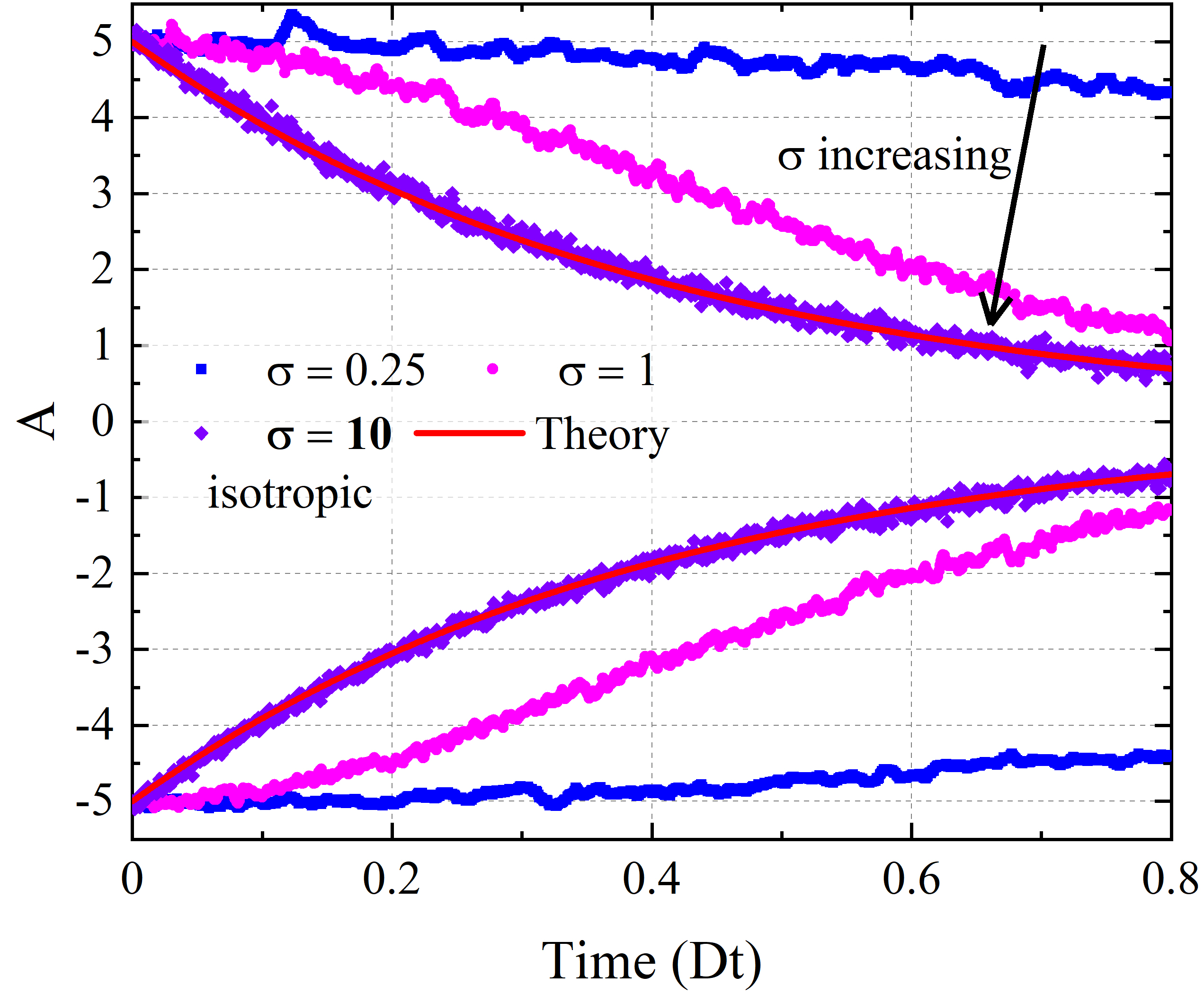
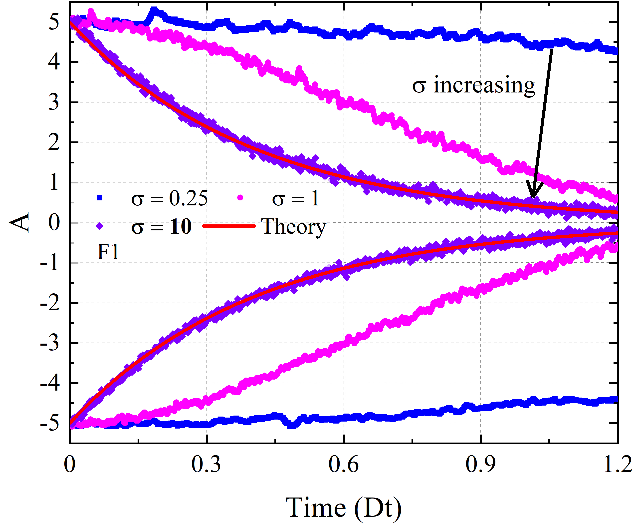
Figure 1: The MC simulated results of the isotropic and F1 scattering cases under different $\sigma$, compared with the theory curve. (a) isotropic scattering, (b) F1 scattering.

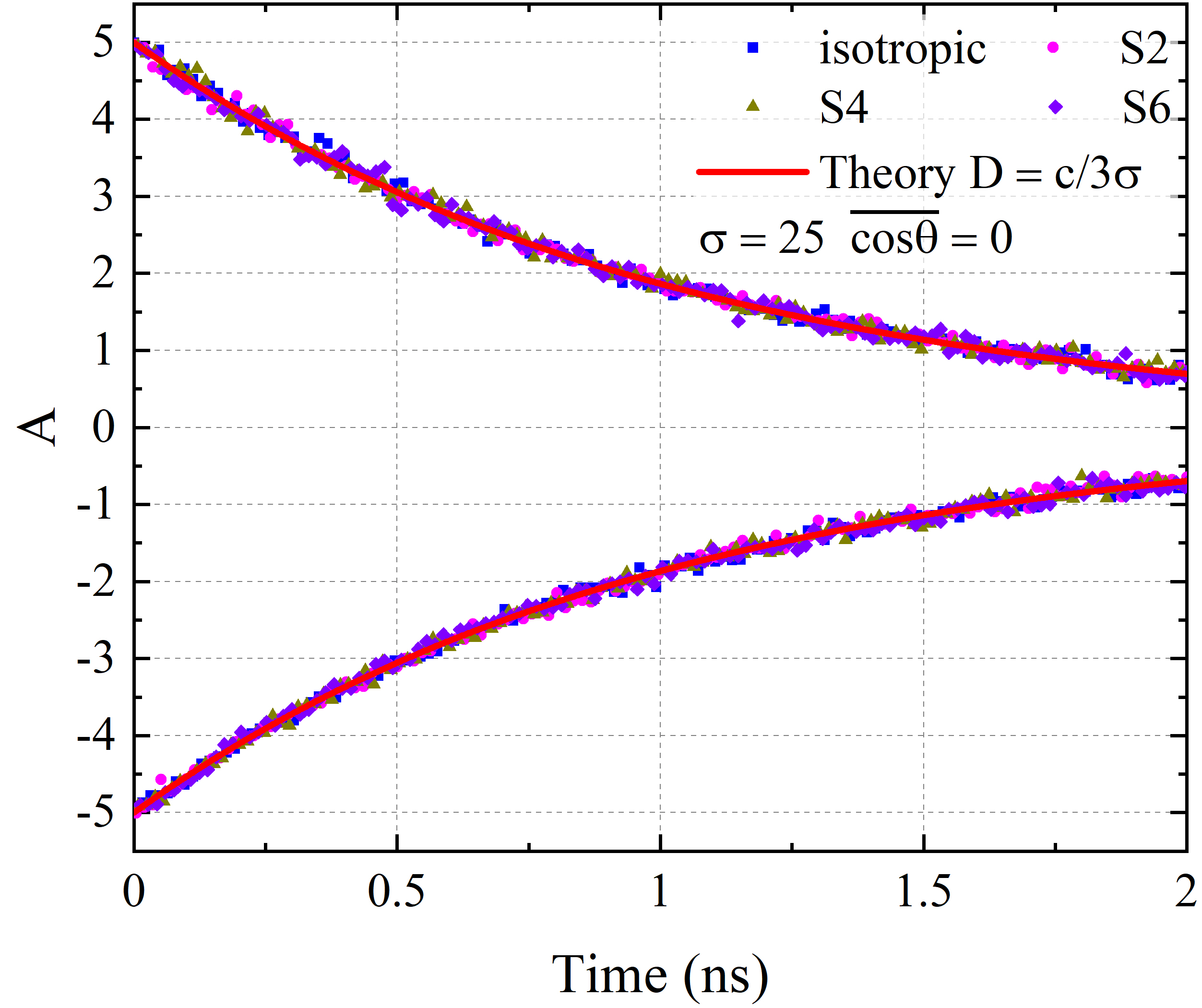
Figure 2: The comparison between the MC simulated results and the theory curve for different scattering phase functions with $\overline{\cos\theta}=0$.

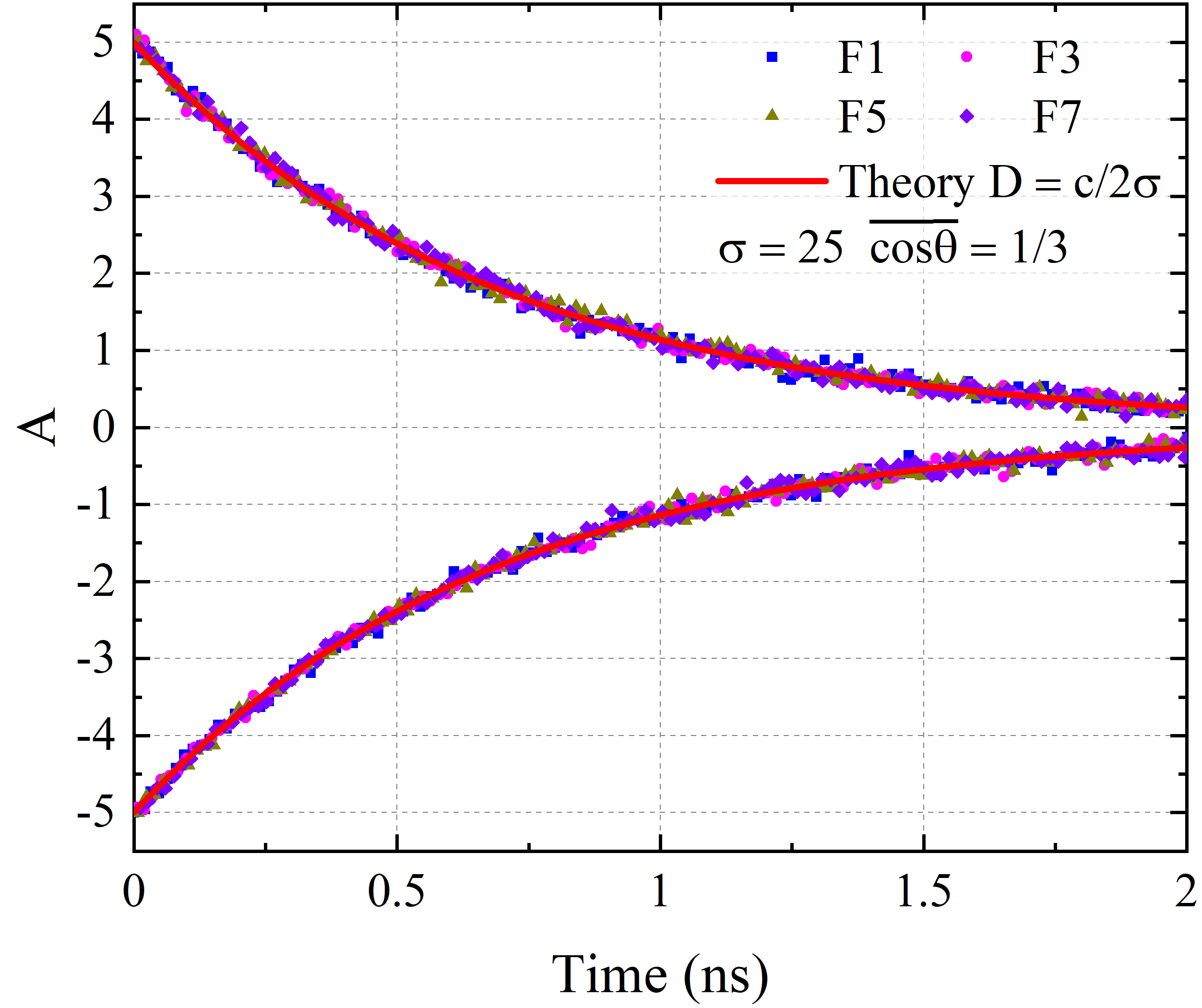
Figure 3: The comparison between the MC simulated results and the theory curve for different, forward scattering phase functions with $\overline{\cos\theta}=1/3$.

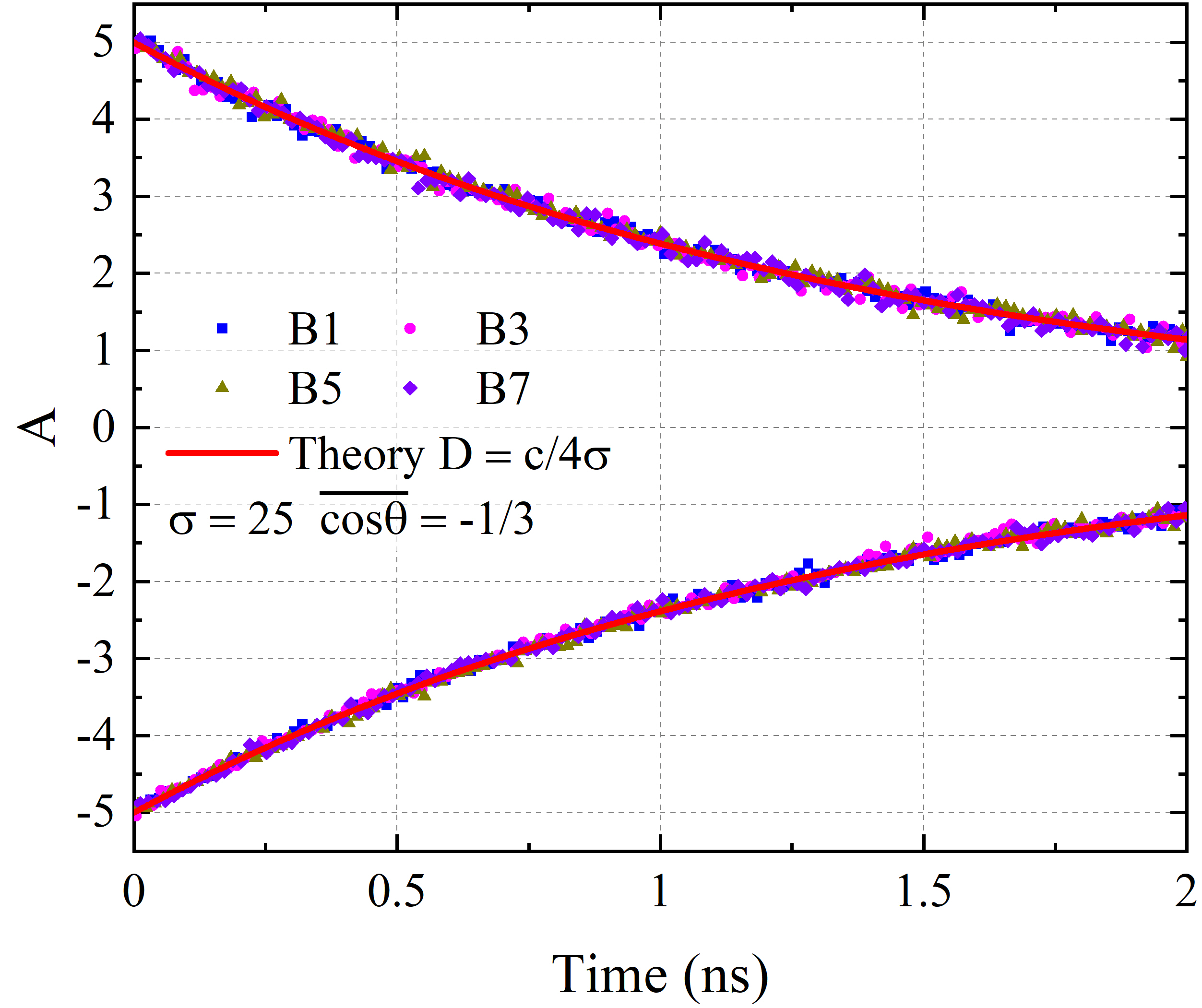
Figure 4: The comparison between the MC simulated results and the theory curve for different backward scattering phase functions with $\overline{\cos\theta}=-1/3$.

Numerical experiments are presented to validate the Theorem II.4. A pure scattering process is considered in a one-dimensional geometry space with periodic boundary conditions. The initial radiation energy distribution of $\rho$ is $\rho=10+5\sin\left(\frac{\pi}{2}x\right),x\in\left[-2,2\right]$. The geometry space has been divided into $10^{3}$ meshes, and the total simulated particles are $10^{7}$. Based on (27), the theoretical prediction of the time evolution of the amplitude follows:

$$A\left(x,t\right)=\rho\left(x,t\right)-10=5\sin\left(\frac{\pi}{2}x\right)e^{-D\left(\frac{\pi}{2}\right)^{2}t}.$$ (38)

We compare the time evolution of amplitude at peak $A(-1,t)$ and valley $A(1,t)$ between the theoretical and numerical results. The phase functions are listed in tables 1-3, where $SL$, $FL$, and $BL$ stand for $L$-th order symmetrical, forward and backward scattering. Figure 1 compares the theoretical predictions and kinetic simulation results of the isotropic and F1 scattering with different $\sigma$, showing a clear convergence to the theoretical curve as $\sigma$ increases. An excellent agreement is observed with $\sigma=10$. Various phase functions are tested as shown in tables (1-3). The kinetic simulation results with scattering parameters $\overline{\cos\theta}=0$, $\overline{\cos\theta}=1/3$ and $\overline{\cos\theta}=-1/3$, with $\sigma=25$, are given in Figure 2-4. Perfect agreement between the theoretical prediction and kinetic simulation data is observed, which validates our reduced model in the optically thick regime.

symbol	phase function	$\overline{\cos\theta}$	D
isotropic	$1/2$	$0$	$c/3\sigma$
$S2$	$3{\cos\theta}^{2}/2$
$S4$	$5{\cos\theta}^{4}/2$
$S6$	$7{\cos\theta}^{6}/2$

Table 1: The corresponding average cosine of the scattering angle and diffusion coefficient of symmetrical scattering phase functions.

symbol	Legendre coefficients	$\overline{\cos\theta}$	D
$F1$	$C_{l=odd}=C_{l=even}=1/2$	$1/3$	$c/2\sigma$
$F3$	$C_{l=odd}=C_{l=even}=1/4$
$F5$	$C_{l=odd}=C_{l=even}=1/6$
$F7$	$C_{l=odd}=C_{l=even}=1/8$

Table 2: The corresponding average cosine of the scattering angle and diffusion coefficient of forward scattering phase functions.

symbol	Legendre coefficients	$\overline{\cos\theta}$	D
$B1$	$-C_{l=odd}=C_{l=even}=1/2$	$-1/3$	$c/4\sigma$
$B3$	$-C_{l=odd}=C_{l=even}=1/4$
$B5$	$-C_{l=odd}=C_{l=even}=1/6$
$B7$	$-C_{l=odd}=C_{l=even}=1/8$

Table 3: The corresponding average cosine of the scattering angle and diffusion coefficient of backward scattering phase functions.

V Conclusion

In the transport process of neutral particle with anisotropic scattering, the even-order scattering kernel will not change the isotropy of the particle velocity distribution. In the highly scattered regime, the high-order transport equation reduces to a low-order diffusion equation. Based on rigorous mathematical derivations, the diffusion coefficient is derived for an arbitrary-order scattering kernel. The numerical experiments show excellent agreement with the theoretical prediction, and a clear physical picture of diffusion is revealed. The theoretical results in this letter contribute to the understanding and simulation of the neutral particle transport physics in the asymptotic optically thick regime.

References

• [1] GJ Boyle, PW Stokes, RE Robson, and RD White. Boltzmann’s equation at 150: Traditional and modern solution techniques for charged particles in neutral gases. The Journal of Chemical Physics, 159(2), 2023.
• [2] Sydney Chapman and Thomas George Cowling. The mathematical theory of non-uniform gases: an account of the kinetic theory of viscosity, thermal conduction and diffusion in gases. Cambridge university press, 1990.
• [3] Jin Hu. Relativistic first-order spin hydrodynamics via the chapman-enskog expansion. Physical Review D, 105(7):076009, 2022.
• [4] Junwu Wang. Continuum theory for dense gas-solid flow: A state-of-the-art review. Chemical Engineering Science, 215:115428, 2020.
• [5] Edward W Larsen and Joseph B Keller. Asymptotic solution of neutron transport problems for small mean free paths. Journal of Mathematical Physics, 15(1):75–81, 1974.
• [6] Edward W Larsen, Jim E Morel, and Warren F Miller Jr. Asymptotic solutions of numerical transport problems in optically thick, diffusive regimes. Journal of Computational Physics, 69(2):283–324, 1987.
• [7] John C Lee. Nuclear Reactor: Physics and Engineering. John Wiley & Sons, 2020.