Supplementary Material for Learning to Drive Anywhere via Regional Channel Attention
Abstract
In this supplementary document, we provide additional implementation details, including network architecture and training protocol, as well as additional analysis, including ablative studies, results on CARLA, and additional qualitative examples. Qualitative results can also be seen in our supplementary video.
1 Implementation Details
This section first provides details regarding our proposed network architecture and discuss differences with baseline models (Sec. 1.1). Next, we provide details regarding the processing of the driving datasets to construct the multi-city benchmark used throughout the analysis (Sec. 1.2). Finally, we discuss evaluation settings (Sec. 1.3) and training protocol (Sec. 1.4).
1.1 Architecture and Baselines
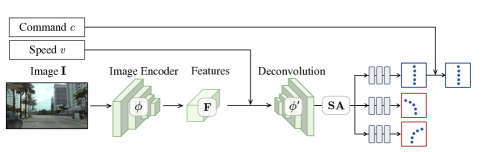
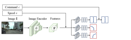
We leverage an ImageNet-pretrained ResNet-34 [He2016CVPR] as our backbone . All images are resized to prior to being inputted to the model. To leverage diverse camera viewpoints, we build on prior models in conditional imitation learning [lbc, zhang2022selfd] and train a direct image-to-BEV prediction model, i.e., without assuming a fixed known BEV perspective transform. Moreover, we also find the removal intermediate image-level heatmaps [lbc, zhang2022selfd] (and directly regressing the BEV waypoints) to improve model performance. Fig. 1 compares our proposed network architecture for image-to-BEV planning to a standard baseline architecture (e.g., [zhang2022selfd, lbc]). Prior image-based models may utilize deconvolutional layers to obtain an image-aligned heatmap and followed by a soft-argmax (‘SA’ in Fig. 1) and 2D waypoint projection to the BEV space. The projection can be implemented either using a homography (i.e., known extrinsic parameters [lbc, wu2022trajectory]) or with a learned projection layer [zhang2022selfd]. In contrast, we find it beneficial to remove the intermediate image-level processing and directly predict BEV waypoints, as shown in Fig. 1(b). We replace the upsampling layers with a convolutional layer which fuses the image and speed-based features prior to inputting to three fully-connected final prediction layers. By removing unnecessary processing steps and enabling more expressive image-to-BEV mappings, the proposed planner architecture improves from 2.45 FDE to 2.17 FDE. This improvement comes with a minimal gain in parameters (23.8M vs. 24.1M). Incorporating the geo-conditional module with three adapters further improves trajectory prediction performance to 1.93 FDE with a 24.2M parameter model. We do not find it necessary to leverage more complex, e.g., GRU-based [wu2022trajectory], prediction heads.
|
| (a) The baseline BEV Planner [zhang2022selfd] relies on alignment with the image input |
| through upsampling (i.e., to obtain a waypoint heatmap), followed by soft-argmax (SA) [lbc]. |
|
| (b) The proposed planner model simplifies the architecture such that each command branch |
| directly predicts BEV waypoints without intermediate upsampling, 2D heatmap, or soft-argmax. |
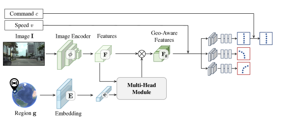 |
| (c) The complete AnyD architecture with geo-aware feature modulation. |
Baselines: While related methods are often studied in simulation [wu2022trajectory, lbc], we provide several baselines by following publicly available implementations. In particular, we leverage the state-of-the-art monocular agent TCP [wu2022trajectory]. To ensure meaningful comparison with single-frame models, we also remove the temporal refinement module. As TCP leverages a control prediction branch in addition to the waypoint prediction branch, we normalize the raw control signals among the different vehicle platforms across the multiple datasets to . When comparing with the semi-supervised learning scheme of SelfD [zhang2022selfd], we leverage a 10-hour YouTube driving dataset with available city (i.e., region) descriptions. In this manner, we are able to use AnyD to pseudo-label videos that were taken within the 11 cities leveraged in our experiments. Subsequently, we mix the datasets to train a semi-supervised AnyD model, which is then evaluated over our multi-city benchmark.
1.2 Data Processing and Distributions
To obtain BEV waypoints for training, we standardize formats across three datasets, Argoverse 2 (AV2) [wilson2021argoverse], nuScenes (nS) [caesar2020nuscenes] and Waymo (Waymo) [sun2020scalability]. The datasets provide post-processed world coordinates for each frame obtained from GPS and other mounted sensors, e.g., LiDAR [caesar2020nuscenes]. We leverage these reported ego-poses to generate a waypoint prediction benchmark. For each frame, we use the global coordinate as an intermediate to get relative positions of the future 2.5s as ground truth waypoints. The conditional command (left, forward, or right) is inferred in a semi-automatic process. First, we extract the preliminary command by thresholding the curvature of the trajectory. However, this process cannot detect subtle maneuvers, such as lane changes, which are included in our dataset. Consequently, we manually verify and annotate the initial automatic command predictions. For our geo-conditional module, we do not require accurate GPS information as we quantize each latitude and longitude into a city-level cluster. Each dataset provides a front-view RGB image and speed (either from the raw CAN bus or from the positioning information), which are inputted into our model as observations.
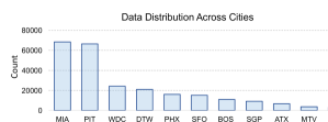
The data spans 11 cities: Pittsburgh (PIT), Washington, DC (WDC), Miami (MIA), Austin (ATX), Palo Alto (PAO) and Detroit (DTW), Boston (BOS), Singapore (SGP), Phoenix (PHX), San Francisco (SFO) and Mountain View (MTV). The data distribution across different cities is shown in Fig. 2.
1.3 Evaluation Metrics and Settings
Open-Loop Evaluation: Average Displacement Error (ADE) and Final Displacement Error (FDE) are standard metrics for trajectory prediction [mangalam2020not]. We first compute the error within each city, and then average to obtain a balanced average metric. We also generate more fine-grained analysis by providing a breakdown over 11 semantic events in the dataset, as will be further discussed in Sec. 2. The extracted events include left turns, forward command, right turns, highway driving, heavy downtown traffic, red traffic lights, stop signs, uncontrolled intersections, pedestrian crossings, rain, and construction zones.
CARLA Evaluation: The open-loop evaluation measures the distance of waypoint predictions with real-world human drivers under complex maneuvers, including yielding, merging, and irregular intersections. To further validate our proposed approach, we sought to evaluate AnyD in closed-loop settings where continuous predictions are made in order to navigate a vehicle to a destination along a route. While closed-loop real-world evaluation is challenging due to safety requirements, we leverage the CARLA [Dosovitskiy17] simulator. Yet, standard CARLA evaluation does not generally involves social and regional behavior that is dynamic across towns. Subsequently, models do not currently incorporate regional modeling, and GPS information is solely used to determine a command at intersections along a route. Hence, motivated by our 11-city real-world benchmark, we introduce a new benchmark where different towns have different traffic behavior. Our benchmark is defined over Town 1, Town 2, and Town 10. We have modified Town 2 for left-hand driving and added pedestrians and vehicles with more aggressive behaviors, e.g., with jaywalking, higher speeds, and closer proximity, to Town 10. We tune the autopilot’s controller in order to generate optimal behavior under the novel settings. When performing closed-loop evaluation in CARLA, we also compute a Driving Score (DS) [carlaleaderboard], which is a product between the route completion and a penalty based on infractions.
1.4 Training Protocol
We study the role of our proposed network for scalable deployment use-cases using three training paradigms. To ensure standardized training across both centralized and federated training, we train the model using Stochastic Gradient Descent (SGD) [acar2021federated]. In centralized training (where all the raw observation data is shared in a single server), we use a batch size of 48 and train for iterations. We set the initial learning rate to -, learning rate decay as , and weight decay as -. The loss hyper-parameters are set as -, -, -. For semi-supervised training settings, model training is done in three stages. We first download a set of online videos based on their tag which provides city-level information. We then train a supervised model using the same hyper-parameters as in centralized training above, and pseudo-label the unlabeled videos. We train three models from different initial seeds to compute a confidence score (i.e., variance) for each pseudo-label and filter low-confidence predictions. Subsequently, we train our model using the original training dataset combined with the large pseudo-labeled dataset. Here, we set the initial learning rate to - and train the model for 500 iterations. Finally, for a fair comparison between the centralized training and the federated training settings, we train our federated model for synchronous communication rounds. We treat each city as its own ‘node’ or ‘device,’ but do not share the private geo-embedding with the server (i.e., we aggregate all model parameters on the server using FedAvg [mcmahan2017communication] and FedDyn [acar2021federated] excluding ). For each communication round, the model is updated for five local iterations with SGD (in this manner, total iterations remain at ). We further note that we remove the geo-contrastive loss term in the federated learning settings (as this information is not shared among the locations). We keep all other hyper-parameters fixed throughout the training settings.
2 Additional Ablation and Results
To supplement our findings in the main paper, we discuss four additional results. First, we provide supplementary analysis in terms of FDE (corresponding to Table 2 of the main paper with ADE), context and event-based performance evaluation (Sec. 2.1). Second, we perform additional ablation studies regarding the role of the number of heads in the multi-head module, impact of GPS noise over waypoints ground-truth in training, and clusters of the neighborhood-level models (Sec. 2.2). Third, we analyze an adaptation experiment to a novel city in Sec. 2.3 and show additional qualitative waypoint prediction results in Sec. 2.5. Finally, we perform closed-loop evaluation results using the introduced CARLA benchmark.
2.1 Additional Analysis
Final Displacement Error: For completeness, we report FDE results across training paradigms and models in Table 1. While FDE is more challenging as it emphasizes long-term prediction, we observe similar trends among the models and cities compared to the complementary ADE-based analysis in the main paper. Specifically, we demonstrate AnyD to improve over our baseline even using this harsher metric, i.e., from 2.55 to 1.93 average FDE. Semi-Supervised Learning (SSL) provides further gains compared to the centralized AnyD for most cities (excluding ATX and DTW, which show slight under-performance). When compared with Federated Learning (FL), the improvement is less pronounced compared to the gains observed with ADE and FL. While some cities are shown to significantly benefit FL over CL (e.g., BOS, SGP, PHX, SFO, MTV) others do not (e.g., MIA and ATX). ATX is a small dataset with limited diversity and high speed variability. While evaluation becomes less reliable, a low-shot learning setting can also be studied to understand such challenges in the future.
| Settings | Methods | Avg | PIT | WDC | MIA | ATX | PAO | DTW | BOS | SGP | PHX | SFO | MTV |
|---|---|---|---|---|---|---|---|---|---|---|---|---|---|
| CL | CIL [lbc] | 2.55 | 2.20 | 2.71 | 2.85 | 2.47 | 3.05 | 2.02 | 1.69 | 2.14 | 3.03 | 3.07 | 2.86 |
| CIRL [liang2018cirl] | 2.48 | 2.39 | 2.55 | 2.82 | 2.37 | 3.13 | 2.21 | 1.61 | 2.03 | 2.59 | 2.88 | 2.72 | |
| BEV Planner [zhang2022selfd] | 2.45 | 2.30 | 2.08 | 2.66 | 2.64 | 3.25 | 2.04 | 1.75 | 2.09 | 2.51 | 2.87 | 2.73 | |
| TCP [wu2022trajectory] | 2.37 | 2.17 | 2.27 | 2.77 | 2.28 | 3.02 | 1.95 | 1.69 | 1.99 | 2.52 | 2.71 | 2.71 | |
| Our Planner | 2.17 | 2.36 | 2.16 | 2.15 | 2.69 | 2.85 | 1.98 | 1.72 | 2.07 | 1.97 | 1.73 | 2.69 | |
| AnyD | 1.93 | 2.19 | 1.97 | 1.94 | 2.48 | 2.83 | 1.80 | 1.55 | 1.96 | 1.88 | 1.62 | 2.80 | |
| SSL | SelfD [zhang2022selfd] | 1.98 | 2.24 | 2.08 | 2.03 | 2.49 | 2.70 | 1.89 | 1.54 | 1.84 | 1.55 | 1.52 | 2.53 |
| AnyD | 1.89 | 2.12 | 1.93 | 1.89 | 2.57 | 2.76 | 1.83 | 1.45 | 1.83 | 1.65 | 1.50 | 2.45 | |
| FL | FedAvg [mcmahan2017communication] | 2.63 | 2.65 | 2.85 | 2.69 | 3.68 | 3.43 | 2.55 | 1.76 | 2.31 | 2.87 | 2.67 | 3.13 |
| FedDyn [acar2021federated] | 2.14 | 2.48 | 2.34 | 2.44 | 3.42 | 3.10 | 2.35 | 1.53 | 1.86 | 1.86 | 1.85 | 2.55 | |
| AnyD (FedAvg) | 2.23 | 2.51 | 2.21 | 2.12 | 3.52 | 3.40 | 2.04 | 1.58 | 2.09 | 2.43 | 1.97 | 2.79 | |
| AnyD (FedDyn) | 1.92 | 2.25 | 1.91 | 1.94 | 3.26 | 3.29 | 1.90 | 1.37 | 1.68 | 1.31 | 1.49 | 2.28 |
| Method | Metric |
Left |
Fwd. |
Right |
Hwy. |
DTown |
Red |
Stop |
Unctrl. |
Cross |
Rain |
Constr. |
|---|---|---|---|---|---|---|---|---|---|---|---|---|
| Our Planner | ADE | 1.60 | 1.01 | 1.43 | 7.66 | 1.12 | 0.66 | 0.63 | 0.77 | 1.36 | 1.37 | 0.76 |
| Full AnyD | 1.48 | 0.92 | 1.19 | 1.37 | 1.04 | 0.60 | 0.66 | 0.72 | 0.80 | 0.80 | 0.56 | |
| Our Planner | FDE | 2.93 | 1.95 | 2.68 | 12.80 | 2.36 | 1.41 | 1.62 | 1.28 | 2.20 | 2.24 | 0.83 |
| Full AnyD | 2.75 | 1.85 | 2.30 | 2.40 | 2.20 | 1.05 | 1.62 | 1.22 | 1.44 | 1.44 | 1.30 |
Event-Driven Analysis: Table 2 shows a breakdown of driving performance over different events and maneuvers. Here, we see a significant benefit for the introduced regional awareness, higher modeling capacity, and more balanced contrastive objective. For instance, AnyD improves performance over the unevenly distributed commands (a ratio of among left:forward:right in our dataset), for right command from 1.43 ADE with the planner and up to 1.19 ADE with AnyD. Other conditions, such as highway, downtown, crossings, and rain conditions all show improvements as well. These results suggest that the situational adapters are able to accommodate various conditions both within and across geo-locations.
2.2 Ablation Studies
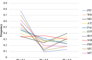
Number of Heads : We investigated the impact of increasing the number of heads in Table 3 on the performance of the model in cities with different amounts of data. We observe that when cities have a sufficient amount of data (defined as more than 10,000 frames), the error rate decreases and remains consistently low as the number of heads increases. This can be attributed to the increased model capacity, allowing for more effective feature extraction and improved learning of city-specific patterns. However, when the training data is limited, increasing the number of heads can still result in worse performance on some of the cities, potentially due to overfitting the small data sample. Thus, efficiently increasing model capacity in small-data domains remains a challenge.
| # of Heads (H) | Large-Data Cities | Small-Data Cities | All Cities |
|---|---|---|---|
| 1 | 1.09 | 1.27 | 1.20 |
| 2 | 1.00 | 1.28 | 1.15 |
| 3 | 0.98 | 1.22 | 1.09 |
| 5 | 1.01 | 1.28 | 1.13 |
| 7 | 1.00 | 1.27 | 1.12 |
Fig. 3 studies the frequency of the head of the highest weight. Notably, our results indicate that the distribution in Singapore, where left-hand driving is practiced, differs from that of other cities. Additionally, the unique tropical scenery of Miami gives rise to a distinctive pattern as well.
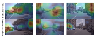
Effects of Geo-Conditional Transformer: Fig. 4 shows the visual effect of the attention pattern of the selected head (head with the highest weight) under the same observations, given different region embeddings. Given Boston embeddings, the head concentrates more on the objects in the middle and right portion of the image. While the Singapore embeddings guide attention towards the left portion of the image, which is attributable to the left-hand driving scenario in Singapore. We note that our supplementary contains additional ablations regarding number of heads in the multi-head attention module and the impact of dataset size on training such higher capacity models.
Ground-Truth Noise Analysis: To understand the role of scalable real-world deployment and data collection, we analyze the impact of potential GPS error in Table 4. While our analyzed datasets carefully post-process the reported world coordinates, we envision AnyD deployed across more diverse and potentially noisy settings. We therefore report the performance degradation due to the addition of 1m and 3m Gaussian noise over the training waypoints. Specifically, we find that even with added noise, AnyD obtains decent prediction performance, outperforming prior state-of-the-art models that are trained with clean waypoints, e.g., 2.39 FDE with 3m noise vs. 2.45 FDE for the baseline [lbc, liang2018cirl]).
| Noise | ADE | FDE |
|---|---|---|
| Original | 1.05 | 1.93 |
| 1.16 | 2.21 | |
| 1.28 | 2.39 |
| of Clusters | PIT | WDC | MIA | ATX | PAO | DTW |
|---|---|---|---|---|---|---|
| 1 | 1.15 | 1.27 | 1.60 | 1.13 | 1.65 | 0.96 |
| 3 | 1.16 | 1.09 | 1.11 | 1.10 | 1.42 | 0.95 |
| 10 | 1.21 | 1.06 | 1.09 | 1.22 | 1.39 | 0.98 |
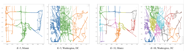
Unsupervised Clustering of Regions: In Table 5, we explore the benefit of finer-grained regional clustering choices, i.e., within each city, when defining . This experiment can uncover potential benefits from modeling intra-city settings. To achieve this, we utilize GPS trace data from OpenStreetMap (OSM)[bennett2010openstreetmap] and cluster cities into sub-regions based on traffic patterns. For example, MIA clustering results in semantic regions, e.g., downtown vs. beach areas, with large improvements in prediction performance for the finer-grained model (from 1.60 to 1.11 ADE). Similarly, WDC is clustered into downtown and highway regions, also benefiting performance (from 1.27 to 1.09 ADE). We note that while these examples suggest our model can further benefit model improvement, such clustering data may not be available for many locations, and thus cannot always be assumed.
Table 5 further explores the benefits of finer-grained clustering on AnyD model performance, i.e., within city neighborhoods. To achieve this, we employ GPS trace data from OpenStreetMap (OSM) [bennett2010openstreetmap] and divide cities into sub-regions based on traffic patterns via K-means clustering. Fig. 5 shows example clustering results in MIA and WDC with respect to and clusters. For instance, the downtown areas of both two cities can be seen as clusters for both and . While somewhat coarse in its clustering, we find that this privileged region information (which may not always be available) can introduce additional benefits when used as during model training and evaluation.
| Cities | Seen Cities (Before After) | GZ |
|---|---|---|
| BEV Planner [zhang2022selfd] | 1.24 1.33 | 0.87 |
| AnyD | 1.05 1.04 | 0.84 |
2.3 Adaptation to a New City
In practice, a geo-aware model may be required to learn to drive in a previously unseen region with a significant domain gap. To understand the model performance of AnyD under such learning settings, we extract an additional city (Guangzhou, China) from a different dataset, ApolloScape [huang2019apolloscape]. In this case, a large domain gap occurs due to the differing social norms and traffic density in China. We mix the new city with the prior 11, and continue fine-tuning the model. Our results in Table 6 indicate that AnyD can learn to drive in the new city while also maintaining similar performance levels for the previously observed cities (i.e., without forgetting). In contrast, the baseline model, which does not incorporate the explicit geo-aware module, has higher error while also impacting performance on prior seen cities.
| Metics | ADE | FDE | SR | RC | IS | DS |
|---|---|---|---|---|---|---|
| BEV Planner [zhang2022selfd] | 0.58 | 0.97 | 0.29 | 0.50 | 0.61 | 0.36 |
| AnyD | 0.46 | 0.79 | 0.36 | 0.69 | 0.67 | 0.50 |
2.4 Experiments on CARLA
The results of the closed-loop experiments on CARLA are shown in Table 7. We find consistent improvements in success rate, route completion, and infractions (the supplementary video shows qualitative examples where the baseline model struggles with left-hand driving). We compute both open and closed-loop metrics by saving the expert actions for the test sequences. AnyD outperforms the baseline planner [zhang2022selfd] on both open-loop metrics (reducing ADE from 0.58 to 0.46) and closed-loop metrics (improving driving score by 38%, from 0.36 to 0.50). Nonetheless, overall success rates are quite low for our benchmark, as it contains significant behavior variability. This highlights the challenging nature of the region-aware decision-making task for current imitation learning models, either in the real-world or in simulation.
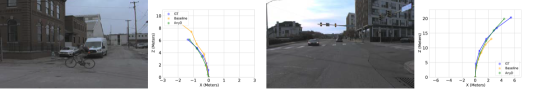
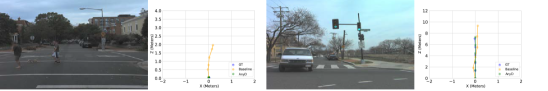
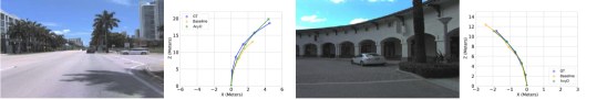
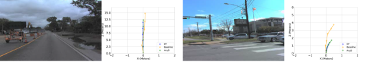
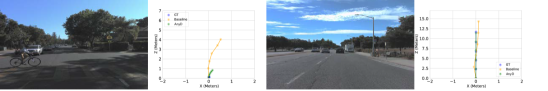
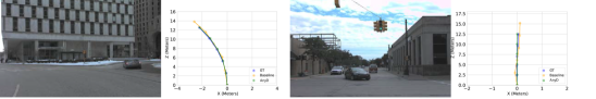
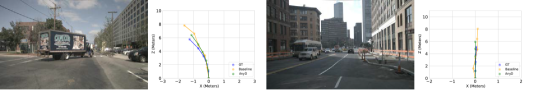
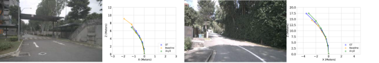
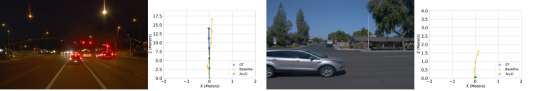
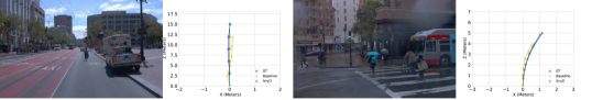
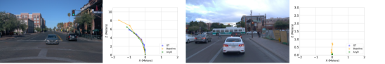
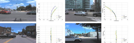
2.5 Qualitative Results
We show additional qualitative results in Fig. 6 and Fig. 7 (on the next page). As depicted in the figures, the AnyD generally provides better performance on challenging tasks of navigating across different regions and events, including turns and merging (requires reasoning over traffic directionality) as well as speed limits. Fig. 8 depicts failure cases, which show challenging conditions involving rare rule violations by other vehicles.