Self-Calibrating, Fully Differentiable NLOS Inverse Rendering

Abstract.

Existing time-resolved non-line-of-sight (NLOS) imaging methods reconstruct hidden scenes by inverting the optical paths of indirect illumination measured at visible relay surfaces. These methods are prone to reconstruction artifacts due to inversion ambiguities and capture noise, which are typically mitigated through the manual selection of filtering functions and parameters. We introduce a fully-differentiable end-to-end NLOS inverse rendering pipeline that self-calibrates the imaging parameters during the reconstruction of hidden scenes, using as input only the measured illumination while working both in the time and frequency domains. Our pipeline extracts a geometric representation of the hidden scene from NLOS volumetric intensities and estimates the time-resolved illumination at the relay wall produced by such geometric information using differentiable transient rendering. We then use gradient descent to optimize imaging parameters by minimizing the error between our simulated time-resolved illumination and the measured illumination. Our end-to-end differentiable pipeline couples diffraction-based volumetric NLOS reconstruction with path-space light transport and a simple ray marching technique to extract detailed, dense sets of surface points and normals of hidden scenes. We demonstrate the robustness of our method to consistently reconstruct geometry and albedo, even under significant noise levels.

1. Introduction

Time-gated non-line-of-sight (NLOS) imaging algorithms aim to reconstruct hidden scenes by analyzing time-resolved indirect illumination on a visible relay surface (Jarabo et al., 2017; Satat et al., 2016; Faccio et al., 2020). These methods typically emit ultra-short illumination pulses on the relay surface, and estimate the hidden scene based on the time of flight of third-bounce illumination reaching the sensor (Velten et al., 2012; O’Toole et al., 2018; Lindell et al., 2019; Xin et al., 2019; Liu et al., 2019).

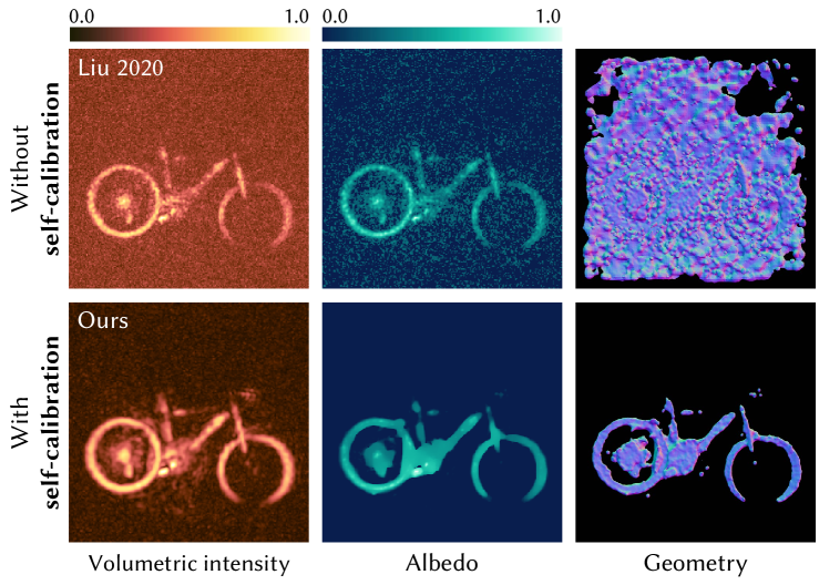
Figure 1. We present a self-calibrating, fully-differentiable NLOS inverse rendering pipeline for the reconstruction of hidden scenes. Our method only requires transient measurements as input and relies on differentiable rendering and implicit surface estimation from NLOS volumetric outputs to obtain the optimal NLOS imaging parameters that yield accurate surface points, normals, and albedo reconstructions of the hidden scene. The top row shows the reconstructed volumetric intensity, albedo, and 3D geometry of a real scene (Liu et al., 2020), failing to reconstruct geometry estimation due to noise interference. The bottom row demonstrates our results after optimization of the imaging parameters.

The majority of existing methods estimate hidden geometry by backprojecting captured third-bounce illumination into a voxelized space that represents the hidden scene (Laurenzis and Velten, 2014), lacking information about surface orientation and self-occlusions (Iseringhausen and Hullin, 2020). Moreover, captured data contains higher-order indirect illumination and high-frequency noise from different sources that introduce undesired artifacts in the reconstructions. Performing a filtering step over the data or the reconstructed volume is the most common solution to mitigate errors and enhance the geometric features (Arellano et al., 2017; Velten et al., 2012; Buttafava et al., 2015; O’Toole et al., 2018; Liu et al., 2019); however, this requires manual design and selection of filter parameters, as their impact in the reconstruction quality is highly dependent on the scene complexity, environment conditions, and hardware limitations.

Recent physically-based methods proposed an alternative technique that avoids the issues linked to backprojection. By merging a simplified but efficient three-bounce transient rendering formula with an optimization loop, the computed time-resolved illumination at the relay wall resulting from an optimized geometry reconstruction is compared to the measured illumination. However, geometric representations introduced by existing works limit the detail in the reconstructions (Iseringhausen and Hullin, 2020) or fail to reproduce the boundaries of hidden objects (Tsai et al., 2019).

Alternatively, the recent development of accurate transient rendering methods (Jarabo et al., 2014; Pediredla et al., 2019; Royo et al., 2022) has fostered differentiable rendering pipelines in path space (Wu et al., 2021; Yi et al., 2021), which have the potential to become key tools in optimization schemes. However, differentiable methods are currently bounded by memory limitations since the need to compute the derivatives of time-resolved radiometric data severely limits the number of unknown parameters that can be handled. The difficulty of handling visibility changes in a differentiable manner, as well as the large number of parameters that need to be taken into account, are two limiting factors shared as well with steady-state differentiable rendering (Li et al., 2018; Zhao et al., 2020), that are further aggravated in the transient regime. As a result, NLOS imaging methods that rely on differentiable rendering are therefore limited to simple operations such as tracking the motion of a single hidden object with a known shape (Yi et al., 2021).

To address these problems, we propose a novel self-calibrated, fully differentiable pipeline for NLOS inverse rendering that jointly optimizes system parameters and scene information to extract surface points, normals, and albedo of the hidden geometry. To this end, we combine diffractive phasor-field imaging in the frequency domain (Liu et al., 2019, 2020) with differentiable third-bounce transient rendering in the temporal domain. We leverage the volumetric output of phasor-field NLOS imaging to estimate geometric information of the hidden scene, which we then use on a transient rendering step to simulate time-resolved illumination at the relay wall. By minimizing the error between simulated and captured illumination, we provide a fully-differentiable pipeline for self-calibrating NLOS imaging parameters in an end-to-end manner.

Our optimized parameters provide accurate volumetric outputs from which we estimate surface points, normals and albedos of hidden objects, with more geometric detail than previous surface-based methods. Our method is robust in the presence of noise, providing consistent geometric estimations under varying capture conditions. Our code is freely available for research purposes.

2. Related Work

Active-light NLOS imaging methods provide 3D reconstructions of general NLOS scenes by leveraging temporal information of light propagation by means of time-gated illumination and sensors (Faccio et al., 2020; Jarabo et al., 2017).

Scene representation

While existing methods rely on inverting third-bounce transport, they may differ in their particular representation of scene geometry as volumetric density or surfaces. Volumetric approaches estimate geometric density by backprojecting third-bounce light paths onto a voxelized space (Velten et al., 2012; Gupta et al., 2012; Buttafava et al., 2015; Gariepy et al., 2015; Arellano et al., 2017; Ahn et al., 2019; La Manna et al., 2018). Efficiently inverting the resulting discrete light transport matrix is not trivial; many dimensionality reduction methods have been proposed (Lindell et al., 2019; Xin et al., 2019; O’Toole et al., 2018; Young et al., 2020; Heide et al., 2019), but they are often limited in spatial resolution (as low as 64$\times$64 in some cases) due to memory constraints. Surface methods, in contrast, rely on inverting third-bounce light transport onto explicit representations of the geometry (Tsai et al., 2019; Iseringhausen and Hullin, 2020; Plack et al., 2023), usually starting with simple blob shapes, progressively optimizing the geometry until loss converges. In contrast, we estimate implicit geometric representations of the hidden scene based on surface points and normals by ray marching the volumetric output of NLOS imaging, inspired by recent work on neural rendering (Mildenhall et al., 2020; Barron et al., 2021; Niemeyer et al., 2022). The combination of NLOS imaging with differentiable transient rendering over the estimated geometry allows us to self-calibrate imaging parameters in an end-to-end manner. For clarity, in this paper the term explicit surface refers to a polygonal surface mesh, while implicit surface denotes a representation based on surface points and their normals, without defining a surface mesh. Please, refer to Section 4.2 for a further detailed discussion on explicit/implicit surface representations.

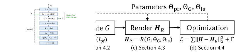
Figure 2. Overview of our self-calibrated, fully differentiable NLOS inverse rendering workflow (Sections 3 and 4). (a) We perform NLOS imaging using a phasor-field diffraction method, taking an initial matrix  $\bm{H}$ of transient measurements as input, and outputting volumetric intensity $I_{\mathrm{pf}}$. (b) We estimate  $G$, an implicit geometric representation of the hidden scene, from $I_{\mathrm{pf}}$. (c) We obtain the time-resolved illumination $\bm{H_{R}}$ from $G$ using differentiable path-space transient rendering. (d) We optimize imaging parameters until the error between $\bm{H}$ and $\bm{H_{R}}$ converges with regularization terms $\Gamma$. Geometry $G$ is computed during the forward pass, while $\Theta_{\mathrm{pf}}$, $\Theta_{\mathrm{ls}}$, and $\Theta_{\mathrm{G}}$ are updated during the backward pass.

Learning-based approaches

Other methods leverage neural networks instead, such as U-net (Grau Chopite et al., 2020), convolutional neural networks (Chen et al., 2020), or neural radiance fields (Mu et al., 2022). These learning-based methods are learned using object databases such as ShapeNet (Chang et al., 2015). However, their parameters are trained with steady-state renderings of synthetic scenes composed of a single object behind an occluder in an otherwise empty space. As such, their performance is often degraded with real scenes, often overfitting to the training dataset, and becoming susceptible to noise. Our method does not rely on a pre-trained deep network to extract high-level features from synthetic steady-state rendering data; instead, we explicitly optimize virtual illumination functions and scene information by evaluating actual transient observations, without relying on neural networks. Recent works by Shen et al. (2021) and Fujimura et al. (2023) leverage transient observations similar to ours for optimizing multi-layer perceptrons for imaging. However, these methods cannot be utilized for calibrating the filtering parameters of volumetric NLOS methods due to the lack of evaluation of the physical observation of the transient measurements by an NLOS imaging and light transport model.

Wave-based NLOS imaging

Recent works have shifted the paradigm of third-bounce reconstruction approaches to the domain of wave optics (Liu et al., 2019; Lindell et al., 2019). In particular, the phasor field framework (Liu et al., 2019) computationally transforms the data captured on the relay surface into illumination arriving at a virtual imaging aperture. This has enabled more complex imaging models (e.g., (Marco et al., 2021; Dove and Shapiro, 2020a, b; Guillén et al., 2020; Reza et al., 2019)), and boosted the efficiency of NLOS imaging to interactive and real-time reconstruction rates (Liu et al., 2020; Nam et al., 2021; Liao et al., 2021; Mu et al., 2022). However, these systems require careful calibration of all their parameters, including the definition of the phasor field and the particular characteristics of lasers and sensors, which makes using them a cumbersome process. Our fully self-calibrated system overcomes this limitation.

3. Time-gated NLOS imaging model

We propose a differentiable end-to-end inverse rendering pipeline (shown in Figure 2) to improve the reconstruction quality of hidden scenes by optimizing the parameters of NLOS imaging algorithms without prior knowledge of the hidden scene. In the following, we describe our NLOS imaging model. Section 4 describes our optimization pipeline based on this NLOS imaging model.

3.1. Phasor-based NLOS imaging

In a standard NLOS imaging setup (see Figure 3), a laser beam is emitted towards a point $\mathbf{x}_{l}$ on a visible relay wall, which reflects light towards the hidden scene and then is reflected back to the wall. The hidden scene is imaged based on the time of flight of the time-resolved illumination, captured at points $\mathbf{x}_{s}$ on the relay wall in the form of a measurement matrix $\bm{H}(\mathbf{x}_{l},\mathbf{x}_{s},t)$.

The recent diffractive phasor-based framework by Liu et al. (2019; 2020) intuitively turns the grid of measured points $\mathbf{x}_{s}$ on the relay wall into a virtual aperture; this allows to formulate the reconstruction of NLOS scenes as a virtual line-of-sight (LOS) problem.

We define $\bm{H}\left(\mathbf{x}_{l},\mathbf{x}_{s},\Omega\right)$ as a set of phasors at the relay wall, obtained by Fourier transform of the measurement matrix $\bm{H}(\mathbf{x}_{l},\mathbf{x}_{s},t)$. In practice, since this function $\bm{H}$ is noisy, we apply a filtering operation as

(1) $$\bm{H}_{\mathrm{pf}}\left(\mathbf{x}_{l},\mathbf{x}_{s},\Omega\right)=\mathcal{P}\left(\mathbf{x}_{l},\mathbf{x}_{s},\Omega\right)\bm{H}\left(\mathbf{x}_{l},\mathbf{x}_{s},\Omega\right),$$

where $\mathcal{P}(\mathbf{x}_{l},\mathbf{x}_{s},\Omega)$ represents a virtual illumination function that acts as a filter over $\bm{H}$, typically defined as a spatially-invariant illumination function (Liu et al., 2019, 2020). The hidden scene can then be imaged as an intensity function $I_{\mathrm{pf}}(\mathbf{x}_{v},t)$ on a voxelized space via Rayleigh-Sommerfeld Diffraction (RSD) operators as

(2) $$I_{\mathrm{pf}}\left(\mathbf{x}_{v},t\right)=\leavevmode\resizebox{377.24727pt}{}{ \mbox{$\left|\int\limits^{\infty}_{-\infty}e^{i\frac{\Omega}{c}{t}}\int\limits_{S}\!\!\int\limits_{L}\frac{e^{-i\frac{\Omega}{c}(d_{lv}+d_{vs})}}{d_{lv}d_{vs}}\bm{H}_{\mathrm{pf}}\left(\mathbf{x}_{l},\mathbf{x}_{s},\Omega\right)\mathrm{d}\mathbf{x}_{l}\mathrm{d}\mathbf{x}_{s}\frac{\mathrm{d}\Omega}{2\pi}\right|^{2},$ } }$$

where $L$ and $S$ define the illuminated and measured regions on the relay wall, respectively; $d_{lv}=\left\|\mathbf{x}_{l}-\mathbf{x}_{v}\right\|$ and $d_{vs}=\left\|\mathbf{x}_{v}-\mathbf{x}_{s}\right\|$ are voxel-laser and voxel-sensor distances (see Figure 3); and $\Omega$ represents frequency.

Classic NLOS reconstruction methods reconstruct hidden geometry by evaluating $\bm{H}(\mathbf{x}_{l},\mathbf{x}_{s},t)$ at the time of flight of third-bounce illumination paths between scene locations and points on the relay surface (O’Toole et al., 2018; Arellano et al., 2017; Gupta et al., 2012). This is analogous to evaluating $I_{\mathrm{pf}}(\mathbf{x}_{v},t)$ at $t=0$, where the RSD propagators have traversed an optical distance $\|\bar{\mathbf{x}}\|=d_{lv}+d_{vs}$. We incorporate a similar third-bounce strategy in our path integral formulation as described in the following. Due to the challenges of estimating surface albedo due to diffraction effects during the NLOS imaging process (Guillén et al., 2020; Marco et al., 2021), we assume an albedo term per surface point that approximates the averaged reflectance observed from all sensor points.

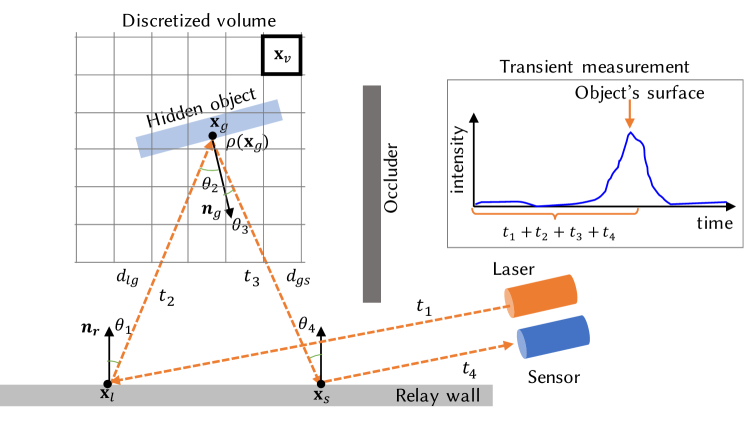
Figure 3. NLOS imaging setup. A laser emits a pulse of light, which travels to the relay wall, then to the hidden geometry, back to the relay wall, and reaches the sensor after a travel time of  $t=t_{1}+t_{2}+t_{3}+t_{4}$. The inset shows the sensor response; the peak at $t$ indicates the presence of a hidden object.

3.2. Path-space light transport in NLOS scenes

To formally describe transient light transport in an efficient manner, we rely on the transient path integral formulation (Jarabo et al., 2014; Royo et al., 2022). Transient light transport $\bm{H}(\mathbf{x}_{l},\mathbf{x}_{s},t)\in\mathbb{R}$ can then be expressed as

(3) $$\bm{H}(\mathbf{x}_{l},\mathbf{x}_{s},t)=\int_{\mathcal{T}}\int_{\psi}\mathcal{K}(\bar{\mathbf{x}},\mathbf{t})\mathrm{d}\mu(\bar{\mathbf{x}})\mathrm{d}\mu(\mathbf{t}),$$

where $\mathcal{K}$ is the radiometric contribution in transient path-space; $\mathrm{d}\mu(\bar{\mathbf{x}})$ is the differential measure of path $\bar{\mathbf{x}}$; $\mathcal{T}$ represents the domain of temporal measurements; $\mathbf{t}=t_{l}\dots t_{s}$ is the sequence of time-resolved measurements on each vertex; $\mathrm{d}\mu(\mathbf{t})$ denotes temporal integration at each vertex; $\bar{\mathbf{x}}=\mathbf{x}_{l}\dots\mathbf{x}_{s}$ is a set of discrete transient path time intervals of $k+1$ vertices; and $\psi=\cup_{k=1}^{\infty}\psi_{k}$ is the entire space of paths with any number of vertices, with $\psi_{k}$ being the space of all paths with $k$ vertices. For convenience and without losing generality, we ignore the fixed vertices at the laser and sensor device in our formulae.

In practice, $\bm{H}$ is obtained by the spatio-temporal integration of transient measurements during a time interval $\tau$, which accounts for the contribution of all paths $\bar{\mathbf{x}}$ with time of flight

(4) $$t=\mathrm{tof}(\bar{\mathbf{x}})=\sum\nolimits_{i=1}^{k}\frac{||\mathbf{x}_{i}-\mathbf{x}_{i-1}||}{c},$$

where $c$ is the speed of light, $\mathbf{x}_{0}\equiv\mathbf{x}_{l}$, and $\mathbf{x}_{k}\equiv\mathbf{x}_{s}$. We assume no scattering delays at the vertices.

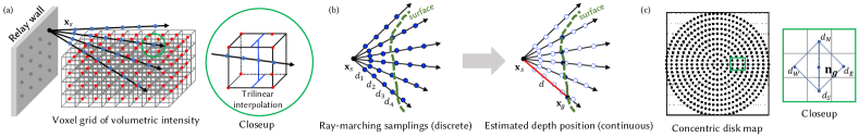
Figure 4. Geometry estimation procedure. (a) We ray-march from sensor points $\mathbf{x}_{s}$, and estimate the intensity at each point along the ray by trilinear interpolation of $I_{\mathrm{pf}}$. (b) From the discrete ray-marching samplings, we obtain a continuous depth function. (c) Normals are computed based on the distances at neighboring ray samples in the concentric hemispherical mapping.

Incorporating the third-bounce strategy of NLOS reconstruction methods in our path integral formulation, we can express $\mathcal{K}$ in a closed form as

(5) $$\mathcal{K}(\bar{\mathbf{x}},\mathbf{t})=\Lambda(\mathbf{x}_{l}\to\mathbf{x}_{g},t_{l})\rho(\mathbf{x}_{g})\mathfrak{T}(\bar{\mathbf{x}},\mathbf{t})\Phi(\mathbf{x}_{g}\to\mathbf{x}_{s},\mathrm{tof}(\bar{\mathbf{x}})),$$

where $\Lambda$ is the emitted light from the laser, $\Phi$ is the time-dependent sensor sensitivity function, $\rho$ represents surface reflectance, and $\mathfrak{T}(\bar{\mathbf{x}},\mathbf{t})$ is the path throughput defined by

(6) $$\mathfrak{T}(\bar{\mathbf{x}},\mathbf{t})=V(\mathbf{x}_{l},\mathbf{x}_{g})\frac{|{\cos{\theta_{1}}||\cos{\theta_{2}}}|}{{d_{lg}^{2}}}V(\mathbf{x}_{g},\mathbf{x}_{s})\frac{|{\cos{\theta_{3}}||\cos{\theta_{4}}}|}{{d_{gs}^{2}}},$$

where $V$ is the binary visibility function between two vertices, $d_{lg}=\|\mathbf{x}_{l}-\mathbf{x}_{g}\|$ and $d_{gs}=\|\mathbf{x}_{g}-\mathbf{x}_{s}\|$, and $\theta_{1-4}$ refer to the angles between the normals of both the relay wall and surface geometry, and the path segments in $\bar{\mathbf{x}}$ (see Figure 3). Note that the three-bounce illumination is expressed in the path space as $\bar{\mathbf{x}}\equiv\mathbf{x}_{l}\rightarrow\mathbf{x}_{g}\rightarrow\mathbf{x}_{s}$.

Neither the emitted light $\Lambda$ nor the sensor sensitivity $\Phi$ are ideal Dirac delta functions. Yi et al. (2021) and Hernandez et al. (2017) provide the following models for the laser and sensor behavior

(7) $${\color[rgb]{0,0,0}{{\Lambda}(t)}} {\color[rgb]{0,0,0}{=\frac{I_{l}}{{\sigma_{l}\sqrt{2\pi}}}{e^{-{{{t}}^{2}}/({2{\sigma_{l}^{2}}})}}}},$$

(8) $${\color[rgb]{0,0,0}{\Phi(t)}} {\color[rgb]{0,0,0}{={\kappa_{s}{e^{-\kappa_{s}t}}}*\frac{1}{{\sigma_{s}\sqrt{2\pi}}}{e^{-{{{(t-\mu_{s})}}^{2}}/({2{\sigma_{s}^{2}}})}}}},$$

where $\sigma_{l}$ is the standard deviation of the Gaussian laser pulse, $I_{l}$ is the laser intensity, $\kappa_{s}$ is the sensor sensitivity decay rate, $\sigma_{s}$ is the standard deviation of the sensor jitter, and $\mu_{s}$ is the offset of the sensor jitter. Since we are only interested on reproducing the combined effect of the laser and sensor models $\Lambda$ and $\Phi$ on the path throughput (Equation 6), we replace them by a single joint laser-sensor correction function as

(9) $$\begin{aligned} {\color[rgb]{0,0,0}{\Psi(t)}}&{\color[rgb]{0,0,0}{=\Phi(t)*\Lambda(t)}}\\ &{\color[rgb]{0,0,0}{={\kappa_{s}{e^{-\kappa_{s}t}}}*\frac{I_{l}}{{\sigma_{ls}\sqrt{2\pi}}}{e^{-{{t}^{2}}/({2{\sigma_{ls}^{2}}})}}.}}\end{aligned}$$

Note that the convolution of the two Gaussian functions of Equations 7 and 8 yields a single Gaussian with a joint model parameter $\sigma_{ls}=\sqrt{{\sigma}_{l}^{2}+{\sigma}_{s}^{2}}$. We set the sensor jitter offset as $\mu_{s}=0$, with the assumption that a uniform distribution of shifts is equally present in all transient measurements. Please refer to the supplemental material for more details on derivation. Our inverse rendering optimization seeks optimal parameters of this model automatically based on physically-based transient rendering.

4. Differentiable Time-gated NLOS Inverse Rendering

In the following, we describe in detail our self-calibrated, end-to-end differentiable inverse rendering pipeline, where the forward pass provides high-detailed reconstructions of the geometry $G$, while the backward pass optimizes per-voxel surface reflectance as albedo $\Theta_{G}$, as well as system parameters $\Theta_{\mathrm{pf}}$ and $\Theta_{\mathrm{ls}}$ to improve the forward pass reconstruction. For clarity, from here on, we redefine our functions in terms of their parameters to be optimized. Refer to the supplemental material for a summary of the different symbols.

4.1. Virtual illumination for RSD propagation

The inputs to our system are the known locations of the illumination $\mathbf{x}_{l}$ and the sensor $\mathbf{x}_{s}$, a matrix  $\bm{H}$ of transient measurements, and an arbitrary virtual illumination function $\mathcal{P}(\Theta_{\mathrm{pf}})\equiv\mathcal{P}(\mathbf{x}_{l},\mathbf{x}_{s},\Omega)$ (Equation 1), where $\Theta_{\mathrm{pf}}$ represents the optimized parameter space for $\mathcal{P}$. Based on previous works (Liu et al., 2019, 2020; Marco et al., 2021), we define $\Theta_{\mathrm{pf}}=\{\sigma_{\mathrm{pf}},\Omega_{\mathrm{pf}}\}$ to model a central frequency with a zero-mean Gaussian envelope as $\mathcal{P}(\Theta_{\mathrm{pf}})=e^{i\Omega_{\mathrm{pf}}t}e^{{-t^{2}}/{(2\sigma_{\mathrm{pf}}^{2})}}$, where $\sigma_{\mathrm{pf}},\Omega_{\mathrm{pf}}$ represent the standard deviation and central frequency, respectively. Note that this equation is fully differentiable. In the forward pass we first compute the filtered matrix $\bm{H}_{\mathrm{pf}}$ (Equation 1) using the optimized virtual illumination $\mathcal{P}(\Theta_{\mathrm{pf}})$, having $\bm{H}_{\mathrm{pf}}=P(\bm{H};\Theta_{\mathrm{pf}})$ (Figure 2a). We then compute a first estimation of the volumetric intensity $I_{\mathrm{pf}}$ of the hidden scene by evaluating RSD propagation (Equation 2) at $t=0$, as $I_{\mathrm{pf}}=RSD(\bm{H}_{\mathrm{pf}})$. Next, we show how to estimate both the geometry $G$ and the time-resolved transport $\bm{H}_{R}$ at the relay wall.

4.2. Implicit surface geometry

Our next goal is to estimate an implicit surface representation $G$ (points $\mathbf{x}_{g}$ and normals $\mathbf{n}_{g}$) by means of a differentiable function $D$ as $G=D(I_{\mathrm{pf}})$ (Figure 2b) that takes our volumetric intensity function $I_{\mathrm{pf}}$ as input.

We keep an implicit representation of our hidden surface geometry $G$ without creating meshed (explicit) surface geometry during the whole optimization. The key idea is to use the volumetric data computed at each forward pass to estimate projections of the geometry (i.e., points and normals) visible from the perspective of each sensor point $\mathbf{x}_{s}$ on the relay wall and use those to perform path-space differentiable transient rendering at $\mathbf{x}_{s}$.

We first estimate the geometry observed by $\mathbf{x}_{s}$ by sampling rays towards our volumetric intensity $I_{\mathrm{pf}}$, and build an implicit representation of the closest surface along each ray. Using information from neighboring rays, we then estimate the normals required to compute the path-space throughput of $\mathfrak{T}$ (Equation 6). Using the implicit geometry computed for every sensing point $\mathbf{x}_{s}$, we then compute time-resolved illumination at $\mathbf{x}_{s}$ as we describe later in this subsection.

Points

As Figure 4a shows, for each sensor point $\mathbf{x}_{s}$ we sample rays uniformly using concentric hemispherical mapping (Shirley and Chiu, 1997). We then sample points along each ray with ray marching, and estimate the intensity at each sampled point (blue in Figure 4a) by trilinear interpolation of neighbor voxel intensities of $I_{\mathrm{pf}}$ (red). From the interpolated volumetric intensities $I_{\mathrm{pf}}(d_{i})$ (Figure 4b, left), we estimate the distance $d_{gs}$ between $\mathbf{x}_{s}$ and the hidden surface vertex $\mathbf{x}_{g}$ (Figure 4b, right), assuming $\mathbf{x}_{g}$ is located at the maximum intensity along the ray. To find $d_{gs}$ in free space from the ray-marched intensities in a differentiable manner, we use softargmax function: $d_{gs}=\frac{{\sum\nolimits_{i}{\omega_{i}{d_{i}}}}}{{\sum\nolimits_{i}\omega_{i}}}$, where $d_{i}$ is a ray-marched distance from $\mathbf{x}_{s}$, and $\omega_{i}={e^{\beta{I_{\mathrm{pf},i}}}}$ is a probability density function of $d_{i}$, and $I_{\mathrm{pf},i}$ is the volume intensity at distance $d_{i}$ along the ray. $\beta$ is a hyperparameter that determines the sensitivity in blending neighboring probabilities, set to 1e+3 in all our experiments. If $I_{\mathrm{pf}}$ falls below a threshold, we assume that no surface has been found; we set this threshold to 0.05 for synthetic scenes, and 0.2 for real scenes throughout the paper. Our procedure implicitly estimates surface points $\mathbf{x}_{g}$ at distances $d=\left\|\mathbf{x}_{s}-\mathbf{x}_{g}\right\|$ by observing via ray marching the grid of phasor-field intensities $I_{\mathrm{pf}}$ from the perspective of the sensing points $\mathbf{x}_{s}$.

Normals

As shown in Figure 4c, we estimate the normal $\mathbf{n}_{g}$ at vertex $\mathbf{x}_{g}$ based on the distances $d_{N},d_{S},d_{E},d_{W}$ at neighboring ray samples in the concentric hemispherical mapping. We compute the normals of two triangles $\triangle d_{N}d_{E}d_{S}$ and $\triangle d_{S}d_{W}d_{N}$ via two edges’ cross product and compute $\mathbf{n}_{g}$ as the normalized sum of the normals of those two triangles.

Surface albedo

Besides points and normals—updated implicitly during each forward pass—, computing path contribution $\mathcal{K}$ (Equation 5) at sensor points $\mathbf{x}_{s}$ requires computing per-point monochromatic albedo $\rho$. We estimate albedos by evaluating the physical observation of the transient measurements in the backward pass.

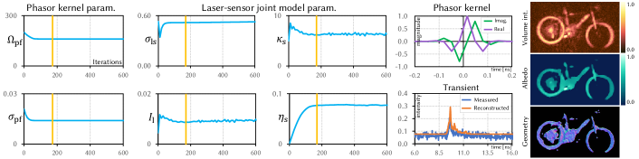
Figure 5. Convergence of the imaging parameters optimized by our method in the Bike real scene. From left to right: Phasor kernel parameters ($\Omega_{\mathrm{pf}}$, $\sigma_{\mathrm{pf}}$), laser-sensor joint model parameters ($\sigma_{\text{ls}}$, $I_{\text{l}}$, $\kappa_{\text{s}}$, $\eta_{\text{s}}$), the converged phasor kernel (purple and green for real and imaginary parts), measured transients compared to our reconstructed one, and our reconstruction results after the optimization. The yellow line indicates when the optimization converges. The converged phasor kernel yields a high-quality reconstruction, while the laser and sensor parameters provide an accurate estimation of transient illumination.

4.3. Differentiable transient rendering

The next step during the forward pass is to obtain time-resolved illumination $\bm{H}_{R}$ at $\mathbf{x}_{s}$ through transient rendering. In our pipeline (Figure 2c), we represent this step as $\bm{H}_{R}=R(G;\Theta_{\mathrm{G}},\Theta_{\mathrm{ls}})$, where $R()$ computes third-bounce time-resolved light transport at sensing points $\mathbf{x}_{s}$. We use the rays sampled from $\mathbf{x}_{s}$ (Figure 4b) to compute the radiometric contribution $\mathcal{K}(\bar{\mathbf{x}},\mathbf{t})$ of the implicit surface points $\mathbf{x}_{g}$ estimated by those rays, following Equations 5 through 9.

Visibility

Differentiating the binary visibility function $V$, necessary to compute the path throughput $\mathfrak{T}$ (Equation 6), is challenging. However, note that we estimate an implicit surface at $\mathbf{x}_{g}$ based on volumetric intensities, which strongly depend on the illumination from the laser reaching the surface and going back to the sensor without finding any occluder. Based on this, we avoid computing the visibility term by assuming the volumetric intensities are a good estimator of the geometry visible from the perspective of both laser and sensor positions on the relay wall.

Transient rendering

The radiometric contribution $\mathcal{K}(\bar{\mathbf{x}},\mathbf{t})$ (Equation 5) yields time-resolved transport in path space for a single path $\bar{\mathbf{x}}\equiv\mathbf{x}_{l}\rightarrow\mathbf{x}_{g}\rightarrow\mathbf{x}_{s}$. Our goal is to obtain a set of discrete transient measurements $\bm{H}_{R}$ from all paths arriving at each sensing point $\mathbf{x}_{s}$, such that $\bm{H}_{R}$ is comparable to the captured matrix $\bm{H}$. To this end, we first discretize $|{\mathcal{K}}(\bar{\mathbf{x}},\mathbf{t})|$ into neighboring bins $\tau$ using a differentiable Gaussian distribution function as ${\mathcal{\hat{K}}}(\bar{\mathbf{x}},\tau)=|{\mathcal{K}}(\bar{\mathbf{x}},\mathbf{t})|\exp\left({-\frac{(\tau-t)^{2}}{2\sigma_{t}^{2}}}\right)$, where $\tau$ is a transient bin index, $t$ is continuous time of $\bar{\mathbf{x}}$ (Equation 4), and $\sigma_{t}$ is set to $0.62$ to make the FWHM of the Gaussian distribution cover a unit time bin.

The time-resolved measurement $\bm{H}_{r}(\mathbf{x}_{l},\mathbf{x}_{s},\tau)$ at temporal index $\tau$ is then approximated as the sum of the discrete path contributions ${\mathcal{\hat{K}}(\bar{\mathbf{x}},\tau)}$ sampled through the concentric disk mapping as

(10) $$\bm{H}_{r}(\mathbf{x}_{l},\mathbf{x}_{s},\tau)\approx\sum\limits_{\bar{\mathbf{x}}\in\mathcal{X}}{\mathcal{\hat{K}}}(\bar{\mathbf{x}},\tau),$$

where $\mathcal{X}$ is the set of paths $\bar{\mathbf{x}}$ that start at $\mathbf{x}_{l}$ and end in $\mathbf{x}_{s}$. After generating the rendered transient data $\bm{H}_{r}$, we then apply our joint laser-sensor model to it to obtain a sensed transient data $\bm{H}_{R}$:

(11) $$\bm{H}_{R}(\mathbf{x}_{l},\mathbf{x}_{s},\tau)=\Psi(\tau)*\bm{H}_{r}(\mathbf{x}_{l},\mathbf{x}_{s},\tau)+\eta_{s}$$

where $\eta_{s}$ is the intensity offset parameter that takes the ambient light and the dark count rate of the sensor into account.

4.4. Optimization of system parameters

Our final goal is to estimate the system parameters $\Theta=\{\Theta_{\mathrm{pf}},\Theta_{\mathrm{ls}},\Theta_{G}\}$ that minimize the loss between the measured matrix $\bm{H}$ and the rendered matrix $\bm{H}_{R}$ (Figure 2, red). We define this as

(12) $$\min_{\Theta}\mathcal{L}(\bm{H},\bm{H}_{R}),$$

which we minimize by gradient descent. The transient cost function $\mathcal{L}$ consists of a data term and regularization terms as

(13) $$\mathcal{L}(\bm{H},\bm{H}_{R})={E_{H}}+{E_{{I_{\mathrm{pf}}}}}+E_{\rho}.$$

The data term $E_{H}$ computes an $l_{2}$ norm between the transient measurements $\bm{H}$ and $\bm{H}_{R}$:

(14) $${E_{H}}=\frac{1}{N_{H}}\sum\limits_{i}{\left\|{{\bm{H}_{i}}-\bm{H}_{R,i}}\right\|_{2}^{2}},$$

where $N_{H}$ is the total number of elements of $\bm{H}$. The key insight of this loss term is that $\bm{H}_{R}$ is the byproduct of time-resolved illumination computed from our implicit geometry $G$, which was itself generated from volumetric intensities $I_{\mathrm{pf}}$ by means of RSD propagation of the ground truth $\bm{H}$. The difference between $\bm{H}$ and $\bm{H}_{R}$ is therefore a critical measure of the accuracy of geometry $G$ and $I_{\mathrm{pf}}$. By backpropagating the loss term through our pipeline, we optimize all system parameters, which improve the estimation of $I_{\mathrm{pf}}$, $G$ and therefore $\bm{H}_{R}$.

The term ${E_{{I}_{\mathrm{pf}}}}$ in Equation 13 is a volumetric intensity regularization term that imposes sparsity, pursuing a clean image:

(15) $${E_{{I_{\mathrm{pf}}}}}=\lambda_{1}\frac{1}{N_{{\mathrm{pf,z}}}}\sum\limits_{j}{\left|{I_{\mathrm{pf,z},j}}\right|},$$

where ${I_{\mathrm{pf,z}}}$ is the maximum intensity values of $I_{\mathrm{pf}}$ projected to the $xz$ plane, $N_{\mathrm{pf,z}}$ is the number of pixels of $I_{\mathrm{pf,z}}$, and $\lambda_{1}$ is a loss-scale balance hyperparameter, which is set to 1e+2 in all our experiments.

The term $E_{\rho}$ in Equation 13 is a regularization term that imposes smoothness, suppressing surface reflectance noise:

(16) $$E_{\rho}=\lambda_{2}\frac{1}{N_{v}}\sum\limits_{m}{\left|{{\nabla_{xy}}{\rho(\mathbf{x}_{v,m})}}\right|},$$

where $N_{v}$ is the number of voxels $\mathbf{x}_{v}$, and $\lambda_{2}$ is a loss-scale balance hyperparameter, which is set to 5e-3 in all our experiments. All terms $E_{H}$, $E_{I_{\mathrm{pf}}}$, and $E_{\rho}$ of the loss function are computed over batches of the transients and voxels at every iteration.

5. Results

We implement our pipeline using PyTorch. Our code runs on an AMD 7763 CPU of 2.45 GHz equipped with a single NVIDIA GPU A100. 3D geometry is obtained from points and normals using Poisson surface reconstruction (Kazhdan and Hoppe, 2013). Please note that we do not perform any thresholding or masking of the data prior to this step. We evaluate our method on four real confocal datasets Bike, Resolution, SU, and 34, provided by O’Toole et al. (2018), Ahn et al. (2019) and Lindell et al. (2019); on two real non-confocal datasets 44i and NLOS, provided by Liu et al. (2019); and on four synthetic confocal datasets Erato, Bunny, Indonesian and Dragon, generated with the transient renderer by Chen et al. (2020). The real datasets include all illumination bounces and different levels of noise depending on their exposure time. The synthetic datasets include up-to third-bounce illumination. In specific cases, we manually add Poisson noise to synthetic datasets to evaluate our robustness to signal degradation.

5.1. Convergence of system parameters

In Figure 5, we show the convergence of our system parameters in a full optimization of the Bike real scene, showing as well the final reconstruction of both volumetric intensity and geometry. Phasor-field kernel parameters $\Omega_{\textrm{pf}}$ and $\sigma_{\textrm{pf}}$ (first column) are responsible for improving the reconstruction quality by constructing a phasor kernel (fourth column, top) that yields high-detailed geometry. The laser and sensor parameters (second and third columns) improve the reconstruction of the transient measurements so that the transient simulation (fourth column, bottom, orange) resembles as much as possible the input data (blue). Refer to the supplemental material for more results of the progressive optimization.

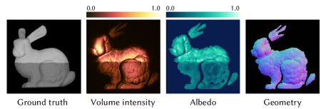
Figure 8. Our optimization scheme estimates spatially-varying albedo in a consistent manner, without affecting the surface and normal estimation. From left to right: Synthetic Bunny scene with two different albedos (0.3 and 1.0), our converged volumetric intensity, the optimized albedo, and the estimated geometry.

Table 1. Ablation study of the impact of each component. MSE transient loss comparison with different configurations with the Bunny scene with two different albedos (Figure 8).

Component			​MSE
Phasor kernel	Albedo	Laser-sensor model	transient
✔	—	—	6.817e-3
✔	—	✔	6.627e-3
—	✔	—	2.239e-3
—	✔	✔	2.217e-3
✔	✔	—	2.124e-3
✔	✔	✔	1.971e-3

We evaluate the impact of each component in our optimization pipeline: phasor kernel, albedo, and laser-sensor model, using a $256\times 256\times 201$ voxel volume. As Table 1 shows, adding albedo and laser-sensor parameters improves the result over just using the phasor parameters, while including the three components yields the best results. The impact of optimizing albedo is the most significant in this experiment.

5.2. Robustness to noise

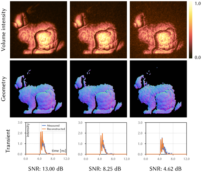
Figure 6. Evaluation of our surface reconstruction under increasing levels of Poisson noise (left to right). From top to bottom: intensity volume, reconstructed geometry, and measured vs. optimized transport. Our method reconstructs geometry reliably across a broad spectrum of noise levels. A lower signal-to-noise ratio (SNR) value indicates a higher level of noise, with an exponential increase in noise.

To illustrate the robustness of our method to signal degradation, in Figure 6 we show reconstructions of the Bunny synthetic dataset under increasing levels of Poisson noise (from left to right) applied to the input transient data. The first row shows the final volumetric reconstruction after the optimization, while the second row shows the resulting surface estimation. The third row shows a comparison between the input transient illumination (blue) and our converged transient illumination at the same location that results from our estimated geometry (orange). The parameters optimized by our pipeline produce a volumetric reconstruction robust enough for our surface estimation method to obtain a reliable 3D geometry under a broad spectrum of noise levels. Note that while the volumetric outputs may show noticeable noise levels (first row), our pipeline optimizes the imaging parameters so that such volumetric outputs provide a good baseline for our geometry estimation method, which yields surface reconstructions that consistently preserve geometric details across varying noise levels (second row).

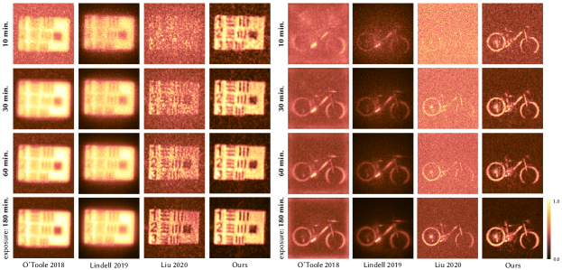
Figure 7. Reconstructed volumetric intensity comparison using the Resolution (left) and Bike (right) real scenes captured under increasing exposure times of 10, 30, 60, and 180 minutes. Existing methods (O’Toole et al., 2018; Lindell et al., 2019; Liu et al., 2020) (first to third columns) fail to reproduce details on the resolution chart across all exposure times, and yield high-frequency noise in the reconstructions due to low SNR in the Bike datasets. Our method (last column) converges to imaging parameters that produce the sharpest results robustly under different exposure times, without requiring manual parameter tuning.

In Figure 7, we compare our method with existing volumetric approaches on two real confocal scenes, Resolution and Bike, captured under different exposure times. For each scene, first to fourth columns illustrate the compared methods: O’Toole et al. (2018), Lindell et al. (2019), Liu et al. (2020), and ours, respectively. First to fourth rows show the resulting volumetric intensity images under increasing exposure times of 10, 30, 60, and 180 minutes, respectively. Our method converges to imaging parameters that produce the sharpest results while significantly removing noise even under the lowest exposure time (top row). Other methods degrade notably at lower exposure times, failing to reproduce details in the resolution chart, or yielding noisy outputs in the Bike scene.

While LCT (O’Toole et al., 2018) allows to manually select an SNR filtering parameter $\alpha$ to improve results in low-SNR conditions, our experiments with different $\alpha$ values from $0.001$ to $1.0$ at different exposure levels validate that our automated calibration approach outperforms the LCT method, reproducing detailed geometric features (see supplemental material).

5.3. Inverse rendering

Our optimization pipeline estimates surface points, normals, and albedo by using only the input transient measurements. Figure 8 illustrates our volumetric intensity, as well as surface points, normals and albedo in the confocal synthetic scene Bunny made of two different surface albedos 1.0 (top) and 0.3 (bottom). Our method is consistent when estimating spatially-varying albedo, while not affecting the estimation of detailed surface points and normals.

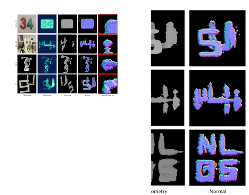
Figure 9. Our inverse rendering results with confocal real scene SU and non-confocal scenes 44i and NLOS. Our approach uses transient measurements to reconstruct surface albedo (second column), geometry (third column), and normals (fourth column), estimating them correctly on multiple isolated objects at different distances.

Figure 9 demonstrates our inverse rendering results on real scenes. As shown in a confocal scene SU (first row) and two non-confocal scenes 44i (second row) and NLOS (third row), we correctly estimate the albedo of objects with uniform reflectance properties (second column), although they undergo different attenuation factors due to being at different distances from the relay wall. The result of the NLOS non-confocal scene (third row) shows the albedo throughout the entire surface is almost identical. Our estimation of surface points and normals (third and fourth columns) is able to accurately reproduce the structure of the hidden geometry.

In Figure 1, we illustrate the benefits of our inverse rendering optimization on the real scene Bike. The first row shows the first iteration of the optimization, which uses the volumetric output by Liu et al. (2020) with the default parameters of the illumination function. The resulting noise heavily degrades the geometry and normal estimation (top-right), and the albedo is wrongly estimated at empty locations in the scene despite the lack of a surface at such locations (top center). After our optimization converges (bottom row), the albedo is estimated only at surface locations, yielding a clean reconstruction of the bike’s surface points and normals.

5.4. Geometry accuracy

In Figure 10, we compare the reconstructed geometry with surface normals in two real scenes (34 and SU) using D-LCT (Young et al., 2020), NeTF (Shen et al., 2021), a differentiable rendering approach (Plack et al., 2023), and our method. Existing methods fail to reproduce detailed surface features in both scenes, such as the subtle changes in depth of the numbers. Plack’s method (fourth column) fails to reproduce the partially occluded U-shaped object and some regions of the S-shaped object in the SU scene. D-LCT (second column) succeeds in reproducing the U-shaped object but fails to reconstruct the detailed geometry of the boundary of the letters. While NeTF (Shen et al., 2021) (third column) is capable of reproducing the U-shaped object, their methodology, based on positional encoding and neural rendering, suppresses geometric details significantly, producing a coarse geometry. Plack’s method faces similar challenges in reproducing geometric details due to the constraints imposed by the resolution of the explicit proxy geometry. Previous optimization-based methods that also rely on explicit geometry (Iseringhausen and Hullin, 2020; Tsai et al., 2019) share similar limitations. Our method based on implicit surface representations is able to handle partial occlusions while reproducing detailed features of the surfaces, such as the depth changes on the numbers and the narrow segments of the letters.

In Figure 11, we provide quantitative comparisons between our estimated geometry and the geometry obtained from D-LCT (Young et al., 2020), NeTF (Shen et al., 2021) and Plack et al. (2023) for three synthetic scenes, Dragon, Erato, and Indonesian, using the Hausdorff distance map as an objective metric. In terms of geometric accuracy, we outperform all three methods in Erato, and Dragon, as shown in the RMSE table. Our improvements are especially noticeable in self-occluded regions and in the reproduction of detailed features. While Plack et al. (2023) yields a lower RMSE in the Indonesian scene, note that it fails to reproduce large regions on the sides of the geometry. Thus, RMSE is only computed on the reconstructed regions and may not fully represent the overall accuracy of the reconstruction.

6. Discussion and Future Work

We have presented an efficient and fully-differentiable end-to-end NLOS inverse rendering pipeline, which self-calibrates the imaging parameters using only the input-measured transient illumination. Our method is robust in the presence of noise while achieving enhanced scene reconstruction accuracy.

Even though forward automatic differentiation (AD) is known to be memory efficient, we implemented our pipeline using reverse AD, as we found it to be 20 times faster and showed better performance when optimizing a large number of parameters (such as per-voxel albedo), and supports a wider set of differentiable functions required for our context.

Phasor-field NLOS imaging can be performed analogously using temporal- or frequency-domain operators (Liu et al., 2019, 2020). However, operating in the temporal domain introduces large memory constraints that are impractical on a differentiable pipeline. Our pipeline therefore operates in the frequency domain to perform NLOS imaging, which provides practical implementation of convolutions of complex-valued phasor-field kernels within GPU memory constraints. While we based volumetric NLOS imaging on phasor-based operators and kernels, an interesting avenue of future work may be optimizing alternative kernel parameterizations or implementing other differentiable NLOS imaging approaches.

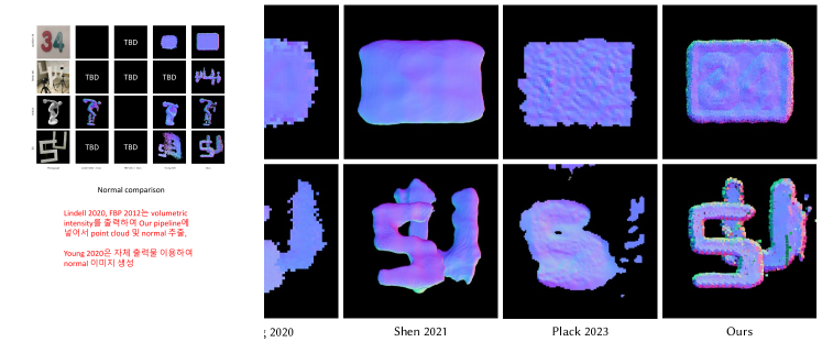
Figure 10. Comparison of the geometry estimation in two real scenes 34 and SU. From left to right: D-LCT (Young et al., 2020), NeTF (Shen et al., 2021), the differential renderer (Plack et al., 2023), and our result. Our method can reconstruct more accurately detailed features such as the depth changes of the numbers, or reproduce narrow segments of the letters, while other methods yield coarse reconstructions or even fail to reproduce partially occluded objects.

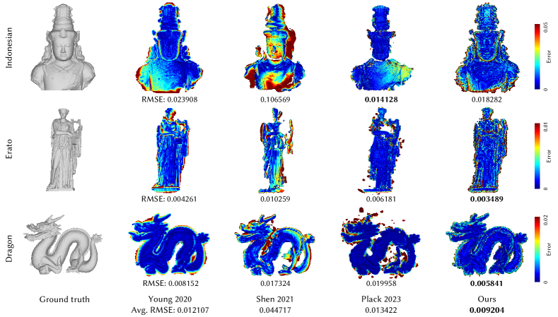
Figure 11. We perform a quantitative comparison of our surface reconstruction with Young et al. (2020), Shen et al. (2021) and Plack et al. (2023) using synthetic transient data with ground truth geometries Dragon, Erato, and Indonesian. We quantify the introduced errors using the Hausdorff distance between the ground truth geometry and the estimated geometries. Our method yields the smallest RMSE in Erato and Dragon, noticeable in highly-detailed areas. Note that while Plack et al. (2023) has smaller RMSE in Indonesian, the reconstructed surface is missing significant regions of the ground truth geometry, which are not quantified by the RMSE.

See pages - of saconferencepapers23-7-supple.pdf