Non-perturbative real topological strings

Abstract

We study the resurgent structure of Walcher’s real topological string on general Calabi–Yau manifolds. We find all-orders trans-series solutions to the corresponding holomorphic anomaly equations, by extending the operator formalism of the closed topological string, and we obtain explicit formulae for multi-instanton amplitudes. We find that the integer invariants counting disks appear as Stokes constants in the resurgent structure, and we provide experimental evidence for our results in the case of the real topological string on local ${\mathbb{P}}^{2}$.

1 Introduction

Topological string theory is defined perturbatively, and it has been a longstanding problem to understand its non-perturbative structure. An important clue for this is the asymptotic behavior of its genus expansion: as in other string theories gp ; shenker , it grows factorially (see e.g. mmlargen ). This usually indicates the existence of exponentially small corrections in the string coupling constant. In the case of conventional strings and minimal strings, it is believed that such effects are due to D-branes polchinski .

In mmopen ; msw ; mmnp it was proposed that a systematic understanding of the non-perturbative effects associated to the divergence of the topological string perturbation series can be obtained by using the theory of resurgence (see ss ; msauzin ; abs ; mmlargen ; mmbook for introductions and reviews). According to this theory, one can associate to the perturbative series a collection of exponentially small corrections, describing non-perturbative amplitudes, together with numerical invariants called Stokes constants (see e.g. gm-peacock for a definition of such a “resurgent structure”). In addition, there is growing evidence that the Stokes constants characterizing the resurgent structure of the topological string free energy are closely related to BPS invariants of the Calabi–Yau (CY) threefold gm-peacock ; astt ; ghn ; gm-multi ; rella ; gkkm ; gu-res ; im (a connection between Stokes constants and BPS invariants has been also found in complex Chern–Simons theory and its supersymmetric 3d duals, see gmp ; ggm1 ; ggm2 ; ggmw ; wheeler ).

The resurgent structure of topological string theory is therefore a very rich object, containing perhaps information about all the BPS invariants of the theory, and a complete description is still lacking. It is possible however to obtain explicit expressions for the non-perturbative corrections by using trans-series solutions to the holomorphic anomaly equations (HAEs) of bcov-pre ; bcov . This idea was put forward in cesv1 ; cesv2 in the local CY case. It was further developed in gm-multi , where exact trans-series solutions in closed form were obtained, and extended to compact CY manifolds in gkkm . The results of gm-multi ; gkkm are based on an operator formalism first considered in coms ; codesido-thesis . One finds in particular that multi-instanton solutions to the HAE are given by a generalization of the eigenvelue tunneling of matrix models david ; shenker ; msw ; multi-multi , which suggests that flat coordinates are quantized in integer units of the string coupling constant.

All the studies done so far focused on closed topological strings. There is a very interesting and rich generalization thereof which we will call the real topological string. Its theory was developed in a series of papers walcher-dq ; walcher-bcov ; walcher-tadpole ; kw-localp2 by J. Walcher and collaborators. The basic idea is to introduce a real three-dimensional locus in the CY target which plays two simultaneous roles: on the one hand it is a submanifold wrapped by a D-brane, giving boundary conditions for open topological strings, and on the other hand it is an orientifold plane, leading in addition to non-orientable amplitudes. Originally, the theory was conceived as involving open and closed strings only walcher-dq ; walcher-bcov , but it was later realized that consistency requires the non-orientable sector as well walcher-tadpole .

The real topological string leads to a perturbative series in the string coupling constant due to a sum over orientable and non-orientable surfaces, with and without boundaries. It is then natural to ask what is the resurgent structure of this series and whether the results of gm-multi ; gkkm can be generalized to this setting. In this paper we start a systematic exploration of these issues. First, we generalize the results of gm-multi ; gkkm and we obtain trans-series solutions to Walcher’s HAE walcher-bcov ; walcher-tadpole for the real topological string. This is achieved by extending the operator formalism of gm-multi ; gkkm . One consequence of our analysis is that multi-instanton solutions to the HAE of the real topological string can be again interpreted in terms of shifts of the closed string background by integer multiples of the string coupling constant. The boundary conditions for the trans-series are provided by the behavior of the real topological string amplitudes at the conifold and the large radius points. As usual in resurgence theory, our results make it possible to obtain the asymptotics of the free energies for large “genus” or Euler characteristic of the worldhseet, which we check successfully against perturbative results in the case of the real topological string on local ${\mathbb{P}}^{2}$. In addition, we find indications that the connection between Stokes constants and BPS invariants extends to the real topological string, and one can explicitly show that the integer invariants counting disks appear as Stokes constants.

This paper is organized as follows. In section 2 we review relevant results about the real topological string, focusing on Walcher’s HAE. Some of the results on the real propagators, like e.g. (2.58), seem however to be new. In section 3 we study the non-perturbative aspects of the theory. We construct trans-series solutions to the HAE by extending the operator formalism of gm-multi ; gkkm to the real case, and we study different boundary conditions for these equations. In section 4 we test the one-instanton amplitude obtained in section 3 in the case of local ${\mathbb{P}}^{2}$. Finally, section 5 contains conclusions and prospects for future studies. Appendix A collects useful results for local ${\mathbb{P}}^{2}$ which are used in the paper.

2 The real topological string

2.1 Free energy and holomorphic anomaly equations

The real topological string involves a CY manifold $X$ together with a D-brane configuration and an orientifold plane. In practice, we consider an antiholomorphic involution of $X$,

$$\sigma:X\rightarrow X.$$ (2.1)

The fixed locus $L$ of $\sigma$ is a Lagrangian submanifold. It can be wrapped by an A-brane, after a choice of an $U(1)$ flat bundle on it, but we can also consider $L$ as an orientifold plane. In the real topological string we have to include the A-brane and the orientifold plane at the same time, as explained in walcher-tadpole .

Example 2.1.

The main example in this paper will be the real topological string on local ${\mathbb{P}}^{2}$, first considered in walcher-tadpole . In this case, $X$ is the total space of the bundle ${\cal O}(-3)\rightarrow{\mathbb{P}}^{2}$. The involution $\sigma$ acts by complex conjugation on both the fiber and the base. The fixed locus $L$ is the total space of the orientation bundle over ${\mathbb{R}}{\mathbb{P}}^{2}$, and since it has $H_{1}(L,{\mathbb{Z}})={\mathbb{Z}}_{2}$, there are two choices for a flat $U(1)$ bundle (or Wilson line). Another example is the quintic CY cdgp , together with an involution which acts again by complex conjugation. Its fixed point locus $L$ is topologically a real projective space ${\mathbb{R}}{\mathbb{P}}^{3}$, and $H_{1}(L,{\mathbb{Z}})={\mathbb{Z}}_{2}$ as well (see e.g. walcher-dq ). ∎

In the real topological string one has to consider contributions from all orientable and non-orientable worldsheet topologies, with and without boundaries. The topological class of the worldsheet is determined by the genus $g\geq 0$, the number of crosscaps $c=0,1,2$, and the number of boundaries $h\geq 0$. The Euler characteristic of such a surface, $\chi$, is given by

$$\chi=2g-2+h+c.$$ (2.2)

The total free energy is obtained as a sum over all possible values of $\chi\geq-2$, and it has the form,

$${\cal G}=\sum_{\chi\geq-2}{\cal G}_{\chi}g_{s}^{\chi}.$$ (2.3)

We will denote by ${\cal F}_{g,h}$ the contribution to ${\cal G}_{\chi}$ coming from orientable Riemann surfaces with genus $g$ and $h$ boundaries, and by ${\cal R}_{g,h}$, ${\cal K}_{g,h}$ the contribution from non-orientable Riemann surfaces of genus $g$ with $h$ boundaries, and $c=1,2$, respectively. We then have

$${\cal G}=\sum_{\chi=2g-2+h}{\cal F}_{g,h}g_{s}^{\chi}+\sum_{\chi=2g-1+h}{\cal R}_{g,h}g_{s}^{\chi}+\sum_{\chi=2g+h}{\cal K}_{g,h}g_{s}^{\chi}.$$ (2.4)

As in walcher-tadpole ; kw-localp2 , we will focus on examples in which ${\cal R}_{g,h}=0$.

The real topological string includes in particular contributions from the conventional closed topological string, corresponding to $c=h=0$. The first new ingredient is the disk amplitude with $g=c=0$, $h=1$, which we will sometimes denote as

$${\cal G}_{-1}={\cal T}.$$ (2.5)

When $H_{1}(L,{\mathbb{Z}})={\mathbb{Z}}_{2}$, as in the examples we will consider, we can interpret ${\cal T}$ as the tension of a BPS domain wall interpolating between the two vacua on the D-brane walcher-dq .

In the A-model, the real topological string provides a generalization of Gromov–Witten theory which “counts” holomorphic maps from open and non-orientable Riemann surfaces to the target space $X$. We recall that, in conventional closed topological string theory, the enumerative information of the Gromov–Witten invariants can be repackaged in terms of integer BPS invariants gv , and the total closed string free energy

$${\cal F}(t;g_{s})=\sum_{g\geq 0}{\cal F}_{g}(t)g_{s}^{2g-2}$$ (2.6)

can be written as

$${\cal F}(t;g_{s})=\sum_{d\in H_{2}(X,{\mathbb{Z}})}\sum_{r\geq 0}\sum_{k=1}^{\infty}n_{r,d}{1\over k}\left(2\sin{kg_{s}\over 2}\right)^{2r-2}{\rm e}^{-kd\cdot t},$$ (2.7)

up to a cubic polynomial in the $t_{i}$s. Here $t=(t_{1},\cdots,t_{s})$ is the vector of complexified Kähler parameters of $X$, and $n_{r,d}$ are the Gopakumar–Vafa invariants, which are integers (see dw for a detailed derivation of (2.7) from a physics perspective). The integrality structure in (2.7) can be extended to the real topological string, and it was proposed in walcher-bcov ; walcher-tadpole ; kw that

$${\cal G}-{\cal F}=2\sum_{r\geq-1}\sum_{d\in H_{2}(X,{\mathbb{Z}})\atop d_{i}\equiv r\,\text{mod}\,2}\sum_{k\,\text{odd}}\tilde{n}_{r,d}{1\over k}\left(2{\rm i}\sin{kg_{s}\over 2}\right)^{r}{\rm e}^{-dk\cdot t/2}.$$ (2.8)

Here, $\tilde{n}_{r,d}$ are new integer invariants counting BPS states. An M-theoretic derivation of this integrality formula has been proposed in pu . As it was emphasized in walcher-tadpole , one has to combine the open and the non-orientable sector to obtain integer invariants $\tilde{n}_{r,d}$. Note however that, when $r=-1$, only disks contribute, and $\tilde{n}_{-1,d}$ can be regarded as an integer counting of disks in $X$ with boundary conditions set by $L$.

As one would expect from mirror symmetry, the calculation of ${\cal G}_{\chi}$ is easier in the B-model. This was first shown in the case of ${\cal T}={\cal G}_{-1}$ in walcher-dq . The domain wall tension is a holomorphic section of the Hodge line bundle ${\cal L}$ over the moduli space of complex structures ${\cal M}$ of $X$. It solves an inhomogeneous Picard–Fuchs equation of the form

$$\mathfrak{L}{\cal T}=f(z_{a}),$$ (2.9)

where $\mathfrak{L}$ is the Picard–Fuchs operator which governs the closed string periods, and $f(z_{a})$ is a known function of the complex moduli. This leads to an efficient counting of disks ending on $L$. The question then arises of how to compute the higher order terms in the real topological string free energy. This problem was solved by Walcher by finding extended HAE for the real topological string, which generalize the closed string case originally studied in bcov-pre ; bcov . In order to present Walcher’s HAE we need to recall some basic ingredients on the special geometry of the CY moduli space ${\cal M}$ (further details can be found in e.g. cdlo ; bcov ; klemm ).

The moduli space ${\cal M}$ of complex structures of the mirror CY is a special Kähler manifold of complex dimension $s$. We will denote by $z^{a}$, with $a=1,\cdots,s$, generic complex coordinates on this moduli space. The Kähler potential will be denoted by $K$, and

$$G_{a\bar{b}}=\partial_{a}\partial_{\bar{b}}K$$ (2.10)

is the corresponding Kähler metric. The line bundle ${\cal L}$ over ${\cal M}$ is endowed with a $U(1)$ connection $A_{a}=\partial_{a}K\equiv K_{a}$, and the covariant derivative $D_{a}$ involves both the Levi–Civita connection associated to the metric,

$$\Gamma^{a}_{bc}=G^{a\bar{k}}\partial_{b}G_{c\bar{k}},$$ (2.11)

and the $U(1)$ connection on ${\cal L}$. Since ${\cal M}$ is a special Kähler manifod, its Christoffel symbols satisfy the special geometry relation

$$\partial_{\bar{b}}\Gamma_{ac}^{d}=G_{a\bar{b}}\delta_{c}^{d}+G_{c\bar{b}}\delta_{a}^{d}-C_{acm}\overline{C}_{\bar{b}}^{md},$$ (2.12)

where $C_{abc}$ is the Yukawa coupling, and

$${\overline{C}}_{\bar{k}}^{ij}={\rm e}^{2K}\,{\overline{C}}_{\bar{k}\bar{a}\bar{b}}G^{i\bar{a}}G^{j\bar{b}}.$$ (2.13)

We recall that, if $\Omega$ is the holomorphic three-form of $X$, the Yukawa coupling is defined by

$$C_{abc}=\int_{X}\Omega\wedge{\partial^{3}\Omega\over\partial z^{a}\partial z^{b}\partial z^{c}}.$$ (2.14)

In topological string theory, it corresponds to the two-sphere amplitude with three insertions.

In the B-model, the free energies ${\cal G}_{\chi}$ get promoted in general to non-holomorphic quantities which we will denote by $G_{\chi}$ (as in gm-multi , non-holomorphic and holomorphic versions of the free energies will written as capital Roman and capital calligraphic letters, respectively). The $G_{\chi}$ are sections of the bundle ${\cal L}^{-\chi}$, and they satisfy Walcher’s HAE. The first ingredient we will need to set up these HAE is the disk two-point function $\Delta_{ij}$, where $i,j$ are moduli indices. Morally, we have

$$\Delta_{ij}\sim D_{i}D_{j}G_{-1}.$$ (2.15)

A more detailed analysis shows that $\Delta_{ij}$ is given by the so-called Griffiths’ infinitesimal invariant walcher-bcov . It can be written in terms of the domain wall tension ${\cal T}$ as

$$\Delta_{ij}=D_{i}D_{j}{\cal T}-{\rm i}C_{ijk}{\rm e}^{K}G^{k\bar{m}}D_{\bar{m}}\overline{{\cal T}}.$$ (2.16)

The Griffiths invariant is not holomorphic, and by using (2.12) one finds that it satisfies the HAE

$$\partial_{\bar{a}}\Delta_{ij}=-{\rm i}C_{ijp}{\rm e}^{K}G^{p\bar{b}}\Delta_{\bar{a}\bar{b}},$$ (2.17)

where

$$\Delta_{\bar{a}\bar{b}}=\overline{\Delta_{ab}}.$$ (2.18)

The Griffiths’ invariant plays the rôle in the open string sector of the Yukawa coupling in the closed string sector. For this reason, it is convenient to introduce its anti-holomorphic version as

$$\Delta_{\bar{a}}^{~{}b}={\rm i}{\rm e}^{K}G^{b\bar{c}}\Delta_{\bar{a}\bar{c}}.$$ (2.19)

We are now ready to consider the HAE for the real topological string in the B-model. As in the closed string case, the one-loop contribution corresponding to $\chi=0$ is somewhat special and needs a separate treatment. There are three different contributions at $\chi=0$: the torus amplitude $F_{1}$, the annulus amplitude $F_{0,2}$, and the Klein bottle amplitude $K_{0,0}$. We first recall that the closed string amplitude at genus one satisfies the HAE bcov-pre ,

$$\partial_{\bar{k}}\partial_{m}F_{1}={1\over 2}{\overline{C}}_{\bar{k}}^{ij}C_{mij}-\left({\chi\over 24}-1\right)G_{\bar{k}m},\$$ (2.20)

where $\chi$ is the Euler number of the CY $X$. The annulus amplitude satisfies walcher-bcov ; walcher-tadpole ,

$$\partial_{\bar{a}}\partial_{j}F_{0,2}=-\Delta_{jk}\Delta_{\bar{a}}^{~{}k}.$$ (2.21)

Finally, the Klein bottle amplitude satisfies, for the type of geometries we will consider walcher-tadpole ,

$$\partial_{\bar{k}}\partial_{m}K_{0,0}={1\over 2}{\overline{C}}_{\bar{k}}^{ij}C_{mij}-G_{\bar{k}m},$$ (2.22)

which is very similar to the HAE for $F_{1}$. In the next section we will solve these equations explicitly in terms of propagators.

We can now write down Walcher’s extended HAE for the real topological string free energies with $\chi\geq 1$ walcher-bcov ; walcher-tadpole . It is given by

$$\partial_{\bar{a}}G_{\chi}={1\over 2}\overline{C}_{\bar{a}}^{P\,jk}\sum\limits_{{\chi_{1}+\chi_{2}=\chi-2}\atop{\chi_{1},\chi_{2}\geq 0}}D_{j}G_{\chi_{1}}D_{k}G_{\chi_{2}}+\overline{C}_{\bar{a}}^{P\,jk}D_{j}D_{k}G_{\chi-2}-\Delta_{\bar{a}}^{P\,j}D_{j}G_{\chi-1},$$ (2.23)

and it applies for $\chi\geq 1$. In these equations, $\overline{C}_{\bar{a}}^{P\,jk}$ and $\Delta_{\bar{a}}^{P~{}j}$ are defined as walcher-tadpole

$$\overline{C}_{\bar{a}}^{P\,jk}=\overline{C}_{\bar{a}}^{jl}{\delta_{l}^{k}+P_{l}^{k}\over 2},\qquad\Delta_{\bar{a}}^{P\,k}=\Delta_{\bar{a}}^{j}{\delta_{j}^{k}+P_{j}^{k}\over 2},$$ (2.24)

and $P_{l}^{k}$ is a projector related to the orientifold action. In the cases we will consider, $P_{l}^{k}=\delta_{l}^{k}$, and $\overline{C}_{\bar{a}}^{P\,jk}=\overline{C}_{\bar{a}}^{jk}$, $\Delta_{\bar{a}}^{P\,j}=\Delta_{\bar{a}}^{j}$. As in the case of the closed topological string, the HAE can be solved recursively starting from the free energy with $\chi=0$ and the “tree level data” given by the Yukawa coupling and Griffith’s invariant. The best procedure to solve these equations is probably the so-called “direct integration” method, developed e.g. in yy ; hk06 ; gkmw ; al . To develop this method, one has to use propagators, which will also play a crucial role in understanding the non-perturbative sectors. They are the subject of the next section.

2.2 Propagators

Propagators were introduced in bcov as a tool to solve the HAE for the closed topological string, and they were generalized in walcher-bcov to solve for (2.23). In this section we will provide a detailed description of the propagators in both the real and the closed case (for the closed case one might consult hosono ; gkkm ). Some of the results for the real propagators seem to be new, and they will be needed in the discussion of the trans-series solution to the extended HAE.

The two-index, closed string propagator is defined by bcov

$$\partial_{\bar{k}}S^{ij}={\rm e}^{2K}\,G^{i\bar{a}}G^{j\bar{b}}{\overline{C}}_{\bar{k}\bar{a}\bar{b}}.$$ (2.25)

In addition to $S^{ab}$ one introduces as well

$$\partial_{\bar{c}}S^{b}=G_{a\bar{c}}S^{ab},\qquad\partial_{\bar{c}}S=G_{a\bar{c}}S^{a}.$$ (2.26)

As in gkkm , we will use the propagator formalism set up in al . We introduce the shifted propagators

$$\tilde{S}^{ij} =S^{ij},$$ (2.27)

$$\tilde{S}^{i} =S^{i}-S^{ij}K_{j},$$

$$\tilde{S} =S-S^{i}K_{i}+\frac{1}{2}S^{ij}K_{i}K_{j}.$$

A fundamental result of bcov ; gkmw ; al is that the derivatives of the propagators w.r.t. the moduli can be written as quadratic expressions in the propagators, and one has the equations

$$\partial_{i}S^{jk} =C_{imn}S^{mj}S^{nk}+\delta_{i}^{j}\tilde{S}^{k}+\delta_{i}^{k}\tilde{S}^{j}-s_{im}^{j}S^{mk}-s_{im}^{k}S^{mj}+h_{i}^{jk},$$ (2.28)

$$\partial_{i}\tilde{S}^{j} =C_{imn}S^{mj}\tilde{S}^{n}+2\delta_{i}^{j}\tilde{S}-s_{im}^{j}\tilde{S}^{m}-h_{ik}S^{kj}+h_{i}^{j},$$

$$\partial_{i}\tilde{S} =\frac{1}{2}C_{imn}\tilde{S}^{m}\tilde{S}^{n}-h_{ij}\tilde{S}^{j}+h_{i},$$

$$\partial_{i}K_{j} =K_{i}K_{j}-C_{ijn}S^{mn}K_{m}+s_{ij}^{m}K_{m}-C_{ijk}\tilde{S}^{k}+h_{ij}.$$

In these equation, $s_{ac}^{r}$, $h_{i}^{jk}$, $h_{ij}$, $h_{i}^{j}$ and $h_{i}$ are holomorphic functions or ambiguities, and they are usually chosen to be rational functions of the moduli. We also have the following important relation between the Christoffel symbols of the Kähler metric, and the propagator $S^{ab}$,

$$\Gamma_{ac}^{r}=\delta_{c}^{r}K_{a}+\delta_{a}^{r}K_{c}-C_{acp}S^{rp}+s_{ac}^{r}.$$ (2.29)

We will need various properties of the closed string propagators. As first pointed out in gkmw , some of these properties are better addressed in the “big moduli space” formalism. In this space, on top of the $s$ complex coordinates $z^{a}$, one introduces an additional complex coordinate corresponding roughly to the string coupling constant. In what follows, lower Latin indices run over $a=1,\cdots,s$, and lower Greek indices run over the indices of the “big” moduli space $\alpha=0,1,\cdots,s$.

In the big moduli space, a crucial role is played by the projective coordinates for the moduli space, $X^{I}$, $I=0,1,\cdots,s$. We recall that a choice of frame in the topological string is equivalent to a choice of a symplectic basis of three-cyles in $H_{3}(X,{\mathbb{Z}})$, $A^{I}$, $B_{I}$, $I=0,1,\cdots,s$. Then, the periods of the holomorphic three-form are defined by

$$X^{I}=\int_{A^{I}}\Omega,\qquad{\cal F}_{I}=\int_{B_{I}}\Omega.$$ (2.30)

The first set of periods defines the projective coordinates, while the second set defines the (projective) prepotential ${\cal F}$ through

$${\cal F}_{I}={\partial{\cal F}\over\partial X^{I}}.$$ (2.31)

We now introduce the $(1+s)\times(1+s)$ matrix (see e.g. gkmw ; klemm ; hosono )

$$\chi^{I}_{\alpha}=\begin{cases}D_{a}X^{I},&\text{if $\alpha=a=1,2,\cdots,s$},\\ X^{I},&\text{if $\alpha=0$.}\end{cases}$$ (2.32)

This matrix is invertible, and its inverse will be denoted by $\chi^{\alpha}_{I}$. It satisfies

$$\chi^{I}_{\alpha}\chi_{J}^{\alpha}=\delta^{I}_{J},\qquad\chi^{I}_{\alpha}\chi_{I}^{\beta}=\delta_{\alpha}^{\beta}.$$ (2.33)

It is shown in hosono that the quantities

$$h_{I}=\chi_{I}^{0}+K_{a}\chi_{I}^{a}$$ (2.34)

are holomorphic.

Let us now consider the holomorphic limit of the theory, which depends on a choice of frame. This is specified by a choice of periods $X^{I}$, $I=0,1,\cdots,s$, and flat coordinates

$$t^{a}={X^{a}\over X^{0}},\qquad a=1,\cdots,s.$$ (2.35)

In the holomorphic limit, one has bcov

$$\Gamma_{ab}^{c}\rightarrow{\partial z^{c}\over\partial t^{p}}{\partial^{2}t^{p}\over\partial z^{a}\partial z^{b}},\qquad K_{a}\rightarrow-\partial_{a}\log(X^{0}).$$ (2.36)

The holomorphic limit of the free energies is obtained by taking the holomorphic limit of the propagators. In the case of the closed string, this limit has been studied in detail in gm-multi ; gkkm . We will denote the holomorphic limit of the shifted propagators by calligraphic letters ${\cal S}^{ij}$, $\tilde{\cal S}^{j}$, $\tilde{\cal S}$. Based on the results in hosono , it can be shown that these holomorphic propagators satisfy the equations

$$C_{ijl}{\cal S}^{lk}-s_{ij}^{k} =-\partial^{2}_{ij}X^{I}\chi_{I}^{k},$$ (2.37)

$$C_{ijk}\tilde{\cal S}^{k}-h_{ij} =h_{I}\partial_{ij}^{2}X^{I}.$$

Let us now introduce propagators for the real topological string, folllowing walcher-bcov . They are defined by

$$\partial_{\bar{a}}R^{b}={\rm i}{\rm e}^{K}G^{b\bar{c}}\Delta_{\bar{a}\bar{c}}=\Delta_{\bar{a}}^{~{}b},$$ (2.38)

and

$$R^{a}=G^{a\bar{b}}\partial_{\bar{b}}R.$$ (2.39)

They are both sections of ${\cal L}^{-1}$. One has also the property

$$\Delta_{\bar{a}\bar{b}}=-{\rm i}\,{\rm e}^{-K}D_{\bar{a}}D_{\bar{b}}R.$$ (2.40)

The propagator $R^{k}$ is closely related to the Griffiths invariant. To see this, we first note that the HAE (2.17) can be written as

$$\partial_{\bar{a}}\Delta_{ij}=-C_{ijk}\Delta_{\bar{a}}^{~{}k},$$ (2.41)

and one has

$$C_{ijk}R^{k}+\Delta_{ij}=d_{ij},$$ (2.42)

where $d_{ij}$ are holomorphic functions. The relation (2.42) is similar to (2.29), and as we will see, it gives a useful expression for the holomorphic limit of the real propagators. As in the closed string case, the derivatives of $R^{j}$, $R$ can be written as polynomials in the propagators. It is convenient to introduce the tilded real propagators al

$$\tilde{R}^{i} =R^{i},$$ (2.43)

$$\tilde{R} =R-K_{i}R^{i}.$$

Since $R^{i}$ remains the same, we will omit the tilde. Then, one finds the relations al

$$\partial_{i}R^{j} =\delta_{i}^{j}\widetilde{R}+S^{jl}\left(C_{ilk}R^{k}-d_{il}\right)-s_{ik}^{j}R^{k}+d_{i}^{j},$$ (2.44)

$$\partial_{i}\widetilde{R} =\left(C_{ijk}R^{j}-d_{ik}\right)\widetilde{S}^{k}-h_{ij}R^{j}+d_{i},$$

where $d_{ij}$, $d_{i}^{j}$ and $d_{i}$ are holomorphic ambiguities and the $d_{ij}$ are the same quantities appearing in (2.42).

It is possible to obtain relations between the real topological string propagators and the closed string propagators. Indeed, by using (2.16), we find

$$\partial_{\bar{a}}R^{b} ={\rm i}{\rm e}^{K}G^{b\bar{c}}D_{\bar{a}}D_{\bar{c}}\overline{\cal T}-\overline{C}_{\bar{a}}^{bm}D_{m}{\cal T}=\partial_{\bar{a}}\left({\rm i}{\rm e}^{K}G^{b\bar{c}}D_{\bar{c}}\overline{\cal T}\right)-\partial_{\bar{a}}S^{bm}D_{m}{\cal T}$$ (2.45)

$$=\partial_{\bar{a}}\left\{{\rm i}{\rm e}^{K}G^{b\bar{c}}D_{\bar{c}}\overline{\cal T}-S^{bm}D_{m}{\cal T}+S^{b}{\cal T}\right\},$$

where we have used that

$$\partial_{\bar{a}}(D_{m}{\cal T})=G_{\bar{a}m}{\cal T},$$ (2.46)

since ${\cal T}$ is holomorphic. A similar argument can be applied to $R$, and one finds in this way,

$$R^{k} =-S^{km}\partial_{m}{\cal T}+\tilde{S}^{k}{\cal T}+{\rm i}\,{\rm e}^{K}G^{k\bar{c}}D_{\bar{c}}\overline{\cal T}+r^{k},$$ (2.47)

$$\tilde{R} =-\tilde{S}^{m}\partial_{m}{\cal T}+2\tilde{S}{\cal T}+{\rm i}\,{\rm e}^{K}\left(\overline{{\cal T}}-K_{b}G^{b\bar{c}}D_{\bar{c}}\overline{\cal T}\right)+r.$$

In these expressions, $r^{k}$, $r$ are holomorphic functions which depend explicitly on the domain wall tension ${\cal T}$. For example, one can show that the functions $r^{k}$ satisfy

$$C_{ijk}r^{k}=-\partial_{ij}^{2}{\cal T}+s^{k}_{ij}\partial_{k}{\cal T}-h_{ij}{\cal T}+d_{ij}.$$ (2.48)

A similar connection between the real and the closed string propagators is implicit in the expressions for the former found in nw in the big moduli space.

Let us now consider the holomorphic limit for the real topological string. In order to do this, we have to understand first the holomorphic limit of Griffiths’ invariant. As explained in walcher-bcov , in a given frame one has to choose ${\cal T}$ in such a way that it vanishes at the appropriate base-point, together with all its holomorphic derivatives. When this is the case, both $\overline{\cal T}$ and $D_{\bar{a}}\overline{\cal T}$ vanish in the holomorphic limit. Therefore, the holomorphic limit of Griffiths’ invariant, which we will denote by ${\cal D}_{ij}$, is simply given by

$${\cal D}_{ij}=D_{i}D_{j}{\cal T},$$ (2.49)

where the covariant derivatives are calculated in the holomorphic limit. In terms of holomorphic propagators, one has

$${\cal D}_{ij}=\partial_{ij}^{2}{\cal T}-\left(C_{ijl}{\cal S}^{lk}-s^{k}_{ij}\right)\partial_{k}{\cal T}+\left(C_{ijk}\tilde{\cal S}^{k}-h_{ij}\right){\cal T}.$$ (2.50)

Let us now consider the holomorphic limit of the real propagators $R^{b}$, $\tilde{R}$ in a given frame. We will use again calligraphic letters and denote these limits by ${\cal R}^{b}$, $\tilde{\cal R}$. They satisfy the holomorphic limits of the various equations that we have considered. For example, from (2.45) we find

$${\cal R}^{k} =-{\cal S}^{km}\partial_{m}{\cal T}+\tilde{\cal S}^{k}{\cal T}+r^{k},$$ (2.51)

$$\tilde{\cal R} =-\tilde{\cal S}^{m}\partial_{m}{\cal T}+2\tilde{\cal S}{\cal T}+r.$$

In adition, by taking the holomorphic limit of (2.42) we obtain,

$$C_{ijk}{\cal R}^{k}-d_{ij}=-{\cal D}_{ij}.$$ (2.52)

As we have emphasized many times, the original propagators are globally defined but non-holomorphic. Their holomorphic limit is frame dependent, and we would like to know how they transform under a change of frame. This was a crucial ingredient in gm-multi ; gkkm and we will need the corresponding generalization to the real case. We recall that a change of frame is implemented by a change of symplectic basis in (2.30) and is therefore associated to a symplectic matrix

$$\Gamma=\begin{pmatrix}A&B\\ C&D\end{pmatrix},$$ (2.53)

where $A$, $B$, $C$, $D$ are $(1+s)\times(1+s)$ matrices which satisfy

$$A^{\rm T}D-C^{\rm T}B={\bf 1}_{s+1},\,\,\,\ A^{\rm T}C=C^{\rm T}A,\,\,\,\ B^{\rm T}D=D^{\rm T}B,$$ (2.54)

and ${\bf 1}_{s+1}$ is the identity matrix of rank $s+1$. The matrix $\Gamma$ acts on the periods as

$$X^{J}_{\Gamma} =C^{JI}{\cal F}_{I}+D^{J}_{~{}I}X^{I},$$ (2.55)

$${\cal F}_{J}^{\Gamma} =A_{J}^{~{}I}{\cal F}_{I}+B_{JI}X^{I}.$$

One can show hosono ; gkkm that the holomorphic shifted propagators in the frame defined by $\Gamma$ are related to the ones in the original frame by the equations,

$${\cal S}^{kl\Gamma} ={\cal S}^{kl}-[(C\tau+D)^{-1}C]^{IJ}\chi_{I}^{k}\chi_{J}^{l},$$ (2.56)

$$\tilde{\cal S}^{k\Gamma} =\tilde{\cal S}^{k}+[(C\tau+D)^{-1}C]^{IJ}\chi_{I}^{k}h_{J},$$

$$\tilde{\cal S}^{\Gamma} =\tilde{\cal S}-{1\over 2}[(C\tau+D)^{-1}C]^{IJ}h_{I}h_{J},$$

where $\chi_{I}^{k}$, $h_{I}$ were introduced in (2.33) and (2.34), respectively.

In the case of the real topological string there is an additional ingredient, since the domain wall tension ${\cal T}$ is in general not invariant under a change of frame. The reason is that, as we change the frame, we want to make sure that the domain wall tension in the new frame, ${\cal T}^{\Gamma}$, as well as its holomorphic derivatives, vanish at the appropriate base-point. The original domain wall tension ${\cal T}$ (or its analytic continuation) does not satisfy this property. In general, ${\cal T}^{\Gamma}$ differs from ${\cal T}$ by a (real) linear combination of periods, i.e.

$${\cal T}^{\Gamma}={\cal T}+\alpha_{I}X^{I}+\beta^{I}{\cal F}_{I}.$$ (2.57)

Note that, since $X^{I}$, ${\cal F}_{I}$ satisfy the homogeneous version of the Picard–Fuchs equation, both ${\cal T}$ and ${\cal T}^{\Gamma}$ solve the defining equation (2.9) for the domain wall tension. We also note that the holomorphic functions $r^{k}$, $r$ appearing in (2.47) will depend on the choice of frame through their dependence on ${\cal T}$.

We will need the transformation properties of the real propagators under a change of frame specified by (2.55) and (2.57). To derive these, we can first deduce the transformation properties of the holomorphic Griffiths invariant (2.50), and then recall the relation (2.52) to derive the transformation of ${\cal R}^{k}$. By using the first equation in (2.44) one finally obtains the transformation of $\tilde{\cal R}$. The final result is,

$${\cal R}^{k\Gamma}-{\cal R}^{k} =\left\{[(C\tau+D)^{-1}C]^{PJ}\partial_{P}{\cal T}^{\Gamma}-\beta^{J}\right\}\chi_{J}^{k},$$ (2.58)

$$\tilde{\cal R}^{\Gamma}-\tilde{\cal R} =-\left\{[(C\tau+D)^{-1}C]^{PJ}\partial_{P}{\cal T}^{\Gamma}-\beta^{J}\right\}h_{J}.$$

In deriving these equations it is useful to keep in mind that, since ${\cal T}$ is a section of ${\cal L}$, it is a homogeneous function of $X^{I}$ of degree one, and Euler’s theorem gives,

$${\cal T}=X^{I}\partial_{I}{\cal T}.$$ (2.59)

As a consequence,

$$\chi^{a}_{I}\partial_{a}{\cal T}+h_{I}{\cal T}=\partial_{I}{\cal T}.$$ (2.60)

2.3 Direct integration

Let us now rewrite Walcher’s HAE in terms of closed and real propagators, following al . Since the non-holomorphic dependence of the free energies is contained in the propagators, one obtains the equations

$${\partial G_{\chi}\over\partial S^{jk}} ={1\over 2}\sum\limits_{{\chi_{1}+\chi_{2}=\chi-2}\atop{\chi_{1},\chi_{2}\geq 0}}D_{j}G_{\chi_{1}}D_{k}G_{\chi_{2}}+D_{j}D_{k}G_{\chi-2},$$ (2.61)

$${\partial G_{\chi}\over\partial R^{i}}-K_{i}{\partial G_{\chi}\over\partial\tilde{R}} =-D_{i}G_{\chi-1},$$

as well as the constraint

$${\partial G_{\chi}\over\partial K_{i}}=0.$$ (2.62)

It is sometimes useful to use HAE for the different ingredients of the total free energy. For example, the oriented open string amplitudes $F_{g,h}$ satisfy walcher-bcov

$$\partial_{\bar{a}}F_{g,h}={1\over 2}\overline{C}_{\bar{a}}^{jk}\sum_{(g_{1},h_{1})+(g_{2},h_{2})=(g,h)}D_{j}F_{g_{1},h_{1}}D_{k}F_{g_{2},h_{2}}+{1\over 2}\overline{C}_{\bar{a}}^{jk}D_{j}D_{k}F_{g-1,h}-R_{\bar{a}}^{j}D_{j}F_{g,h-1},$$ (2.63)

which leads to

$${\partial F_{g,h}\over\partial S^{jk}} ={1\over 2}\sum_{(g_{1},h_{1})+(g_{2},h_{2})=(g,h)}D_{j}F_{g_{1},h_{1}}D_{k}F_{g_{2},h_{2}}+{1\over 2}D_{j}D_{k}F_{g-1,h},$$ (2.64)

$${\partial F_{g,h}\over\partial R^{i}}-K_{i}{\partial F_{g,h}\over\partial\tilde{R}} =-D_{i}F_{g,h-1},$$

and the constraint

$${\partial F_{g,h}\over\partial K_{i}}=0.$$ (2.65)

Similarly, one can write HAE for the non-orientable amplitudes separately.

We can now use the propagators to write explicit expressions for the free energies. Let us first consider the exceptional case with $\chi=0$. In the case of the genus one free energy $F_{1}$, we can use the definition of the propagator to integrate (2.20) as

$$D_{i}F_{1}={1\over 2}C_{ijk}S^{jk}-\left({\chi\over 24}-1\right)K_{i}+f^{(1)}_{i}(z),$$ (2.66)

where $f^{(1)}_{i}(z)$ is a holomorphic ambiguity. A similar formula can be obtained for the Klein bottle amplitude,

$$D_{i}{\cal K}_{0,0}={1\over 2}C_{ijk}S^{jk}-K_{i}+k^{(1)}_{i}(z),$$ (2.67)

where $k^{(1)}_{i}(z)$ is the corresponding ambiguity. Finally, for the annulus amplitude one obtains from (2.21), in terms of real propagators,

$$\partial_{j}F_{0,2}={1\over 2}C_{jkl}R^{k}R^{l}-d_{jk}R^{k}+f_{j}^{(0,2)}(z),$$ (2.68)

where $f_{j}^{(0,2)}(z)$ is the holomorphic ambiguity. By adding all these results, we obtain a useful formula for the derivative of the total $\chi=0$ amplitude,

$$\partial_{j}G_{0}=C_{jlk}S^{kl}-{\chi\over 24}K_{j}+{1\over 2}C_{jkl}R^{l}R^{k}-d_{jk}R^{k}+g_{j}^{(0)}.$$ (2.69)

Let us note that, when acting on $G_{0}$, $D_{j}=\partial_{j}$. The result (2.69) can be used in the HAE (2.61) to calculate all the $G_{\chi}$ recursively, as polynomials in the propagators, and up to holomorphic ambiguities. Let us work out the first case, $G_{1}$. It satisfies the equations

$${\partial G_{1}\over\partial S^{ij}} =\Delta_{ij}=-C_{ijk}R^{k}+d_{ij},$$ (2.70)

$${\partial G_{1}\over\partial R^{j}}-K_{j}{\partial G_{1}\over\partial\tilde{R}} =-D_{j}G_{0}.$$

By using (2.69) the last equation can be split into two,

$${\partial G_{1}\over\partial R^{k}} =-C_{ijk}S^{ij}-{1\over 2}C_{kij}R^{i}R^{j}+d_{kj}R^{j}+g_{k}^{(0)},$$ (2.71)

$${\partial G_{1}\over\partial\tilde{R}} =-{\chi\over 24}.$$

By integrating these equations, we obtain

$$G_{1}=-S^{ij}\left(C_{ijk}R^{k}-d_{ij}\right)-{1\over 6}C_{ijk}R^{i}R^{j}R^{k}+{1\over 2}d_{ij}R^{i}R^{j}-{\chi\over 24}\tilde{R}+g_{k}^{(0)}R^{k}+g_{1},$$ (2.72)

where $g_{1}$ is a new holomorphic ambiguity.

2.4 Fixing the holomorphic ambiguity

Integrating the HAE for the real topological string requires fixing the holomorphic ambiguity at each value of $\chi$. As in the closed string case, in order to do this it is helpful to know the behavior of the real topological string amplitudes at special points in moduli space. Among these, perhaps the most important one is the conifold locus. It has been known for some time that closed topological string amplitudes have a universal behavior at this locus, given by the $c=1$ string gv-conifold . Let us assume for simplicity that there is a single modulus in the geometry, and let $t_{c}$ be a vanishing flat coordinate at the conifold locus. Then, in the conifold frame, the closed string amplitudes have the following behavior,

$${\cal F}_{g}^{c}(t_{c})={B_{2g}\over 2g(2g-2)}t_{c}^{2-2g}+{\cal O}(1),$$ (2.73)

where $B_{2g}$ are Bernoulli numbers, and we have normalized $t_{c}$ appropriately (here and in the following we use inhomogeneous free energies, which differ from the homogeneous ones in an appropriate power of $X^{0}$). According to (2.73) there are no subleading poles in the free energy near the conifold point. This gap condition was emphasized in hk06 and it was later realized that, in many toric CY manifolds, it makes it possible to fix the holomorphic ambiguity at all genera hkr .

The behavior of the real topological string amplitudes near the conifold point was studied in walcher-bcov ; walcher-tadpole ; kw-localp2 ; kw . It was found that all real topological string amplitudes ${\cal F}_{g,h}$, ${\cal K}_{g,h}$ with $h\not=0$ were regular at the conifold point, except for ${\cal K}_{g,0}$, which in the conifold frame and near the conifold point behaves as

$${\cal K}^{c}_{g-1,0}(t_{c})={\Psi_{g}\over t_{c}^{2g-2}}+{\cal O}(1).$$ (2.74)

A proposal for the value of the coefficient $\Psi_{g}$ was made in kw , and it is given by

$$\Psi_{g}={1\over 2^{2g+1}g(g-1)}\left\{-(2^{2g}-1)B_{2g}+gE_{2g-2}\right\},$$ (2.75)

where $B_{2g}$ are Bernoulli numbers and $E_{2g-2}$ are Euler numbers. We conclude that ${\cal G}_{\chi}$ has a gap behavior at the conifold for $\chi$ even, and is regular for $\chi$ odd. This behavior helps in fixing the holomorphic ambiguity, but in contrast to what happens in the closed string case, it does not fix it completely, even in the local case, and one has to use further information. We will discuss this in more detail in section 4.

3 Trans-series solutions and resurgent structure

Our discussion of the real topological string has so far focused on its perturbative expansion. Following cesv1 ; cesv2 ; cms ; gm-multi ; gkkm , we would like to consider now trans-series solutions to Walcher’s HAE. These will be used to obtain information on the non-perturbative sector of the real topological string, and in particular to find explicit multi-instanton amplitudes.

3.1 Master equation and warm-up example

In order to obtain a trans-series solution we have to re-express first the HAE as a “master equation” for the full free energy $G$. Due to the special rôle of the $G_{\chi}$ with $-2\leq\chi\leq 0$, we have to consider four different generating series, which we define as

$$G^{(0)} =\sum_{\chi\geq-2}G_{\chi}g_{s}^{\chi},\qquad\widetilde{G}^{(0)}=\sum_{\chi\geq-1}G_{\chi}g_{s}^{\chi},$$ (3.1)

$$\widehat{G}^{(0)} =\sum_{\chi\geq 0}G_{\chi}g_{s}^{\chi},\qquad\overline{G}^{(0)}=\sum_{\chi\geq 1}G_{\chi}g_{s}^{\chi}.$$

The superscript ⁽⁰⁾ indicates that these are all perturbative amplitudes, and the overline in the last series should not be confused with complex conjugation. We will first consider the following trans-series ansatz to solve the HAE,

$$G=\sum_{\ell\geq 0}{\cal C}^{\ell}G^{(\ell)},$$ (3.2)

where ${\cal C}$ is a formal parameter keeping track of the exponential weight, and

$$G^{(\ell)}=\sum_{n\geq 0}{\rm e}^{-\ell{\cal A}/g_{s}}G_{n}^{(\ell)}g_{s}^{n},\qquad\ell\geq 1.$$ (3.3)

We will often refer to ${\cal A}$ as an “instanton action” and to the $G^{(\ell)}$ as $\ell$-th instanton amplitudes (a more general ansatz will be considered below, in section 3.4). Our goal is to find explicit expressions for the amplitudes $G^{(\ell)}$. We define the trans-series analogue of $\widetilde{G}^{(0)}$ as

$$\widetilde{G}=\widetilde{G}^{(0)}+\sum_{\ell\geq 1}{\cal C}^{\ell}G^{(\ell)},$$ (3.4)

and similarly for $\widehat{G}$ and $\overline{G}$.

Before working out the general trans-series solution, it is instructive to solve a simple, particular case by hand, as it was done originally in cesv1 ; cesv2 . The simplest situation is the one considered in gm-multi for closed topological strings, namely toric or local CY manifolds with a single modulus. In the local case, as first noted in kz , the HAE simplify substantially: the holomorphic limit of $K_{a}$ vanishes, and the closed string propagators $\tilde{\cal S}^{k}$, $\tilde{S}$ can be set to zero by an appropriate choice of the holomorphic functions appearing in the equations (2.28). Similarly, one can set to zero the holomorphic real topological string propagator $\tilde{\cal R}$ by choosing $h_{ij}=d_{i}=0$, as required by the second equation in (2.44). Therefore, if we are interested in the end in calculating holomorphic quantities, we can set $\tilde{S}^{k}$, $\tilde{S}$ and $\tilde{R}$ to zero from the very beginning. Since we want to consider a single modulus case, there are only two non-zero propagators, namely $S^{zz}$ and $R^{z}$. Taking all this into account, the HAE (2.61) simplify to

$${\partial G_{\chi}\over\partial S^{zz}} =\frac{1}{2}\sum\limits_{{\chi_{1}+\chi_{2}=\chi-2}\atop{\chi_{1},\chi_{2}\geq 0}}D_{z}G_{\chi_{1}}D_{z}G_{\chi_{2}}+D^{2}_{z}G_{\chi-2},$$ (3.5)

$${\partial G_{\chi}\over\partial R^{z}} =-D_{z}G_{\chi-1}.$$

We first write down master equations for the perturbative series, and we then postulate that these equations are valid for their trans-series counterparts. It is easy to see that one obtains in this way,

$${\partial\overline{G}\over\partial S^{zz}} ={g_{s}^{2}\over 2}\left(D_{z}\widehat{G}\right)^{2}+g_{s}^{2}D_{z}^{2}\widetilde{G},$$ (3.6)

$${\partial\overline{G}\over\partial R^{z}} =-g_{s}D_{z}\widehat{G}.$$

We will focus in this section on the one-instanton amplitude. It satisfies the linearized master equations

$${\partial G^{(1)}\over\partial S^{zz}} =g_{s}^{2}D_{z}\widehat{G}^{(0)}D_{z}G^{(1)}+g_{s}^{2}D_{z}^{2}G^{(1)},$$ (3.7)

$${\partial G^{(1)}\over\partial R^{z}} =-g_{s}D_{z}G^{(1)}.$$

We now plug in these equations the ansatz (3.3) and we solve order by order in $g_{s}$. We find that, as in the closed topological string case cesv1 ; cesv2 , ${\cal A}$ is independent of the propagators. The next order gives the following equations for $G_{0}^{(1)}$:

$${\partial G_{0}^{(1)}\over\partial S^{zz}} =(\partial_{z}{\cal A})^{2}G_{0}^{(1)},$$ (3.8)

$${\partial G_{0}^{(1)}\over\partial R^{z}} =\partial_{z}{\cal A}\,G_{0}^{(1)}.$$

This can be immediately integrated to obtain

$$G_{0}^{(1)}=\exp\left((\partial_{z}{\cal A})^{2}S^{zz}+\partial_{z}{\cal A}\,R^{z}\right)g_{0}^{(1)},$$ (3.9)

where $g_{0}^{(1)}$ is independent of the propagators, and it is the trans-series counterpart of the holomorphic ambiguity. As first explained in cesv1 ; cesv2 , this ambiguity is fixed by evaluating the trans-series in a special frame, called the ${\cal A}$-frame. This is a frame in which ${\cal A}$ is one of the $A$-periods. In this frame we impose a fixed, simple form for the multi-instanton amplitude, which we will call, as in gm-multi ; gkkm , a boundary condition. We will discuss different boundary conditions in section 3.5. In the case at hand, as we will explain below, the boundary condition is simply

$${\cal G}_{0,{\cal A}}^{(1)}=1,$$ (3.10)

where the subscript ${\cal A}$ means evaluation in the ${\cal A}$-frame. On the other hand, from the above expression we find

$${\cal G}_{0,{\cal A}}^{(1)}=\exp\left((\partial_{z}{\cal A})^{2}{\cal S}^{zz}_{\cal A}+\partial_{z}{\cal A}\,{\cal R}^{z}_{\cal A}\right)g_{0}^{(1)},$$ (3.11)

and this fixes $g_{0}^{(1)}$. We obtain in the end

$$G_{0}^{(1)}=\exp\left((\partial_{z}{\cal A})^{2}(S^{zz}-{\cal S}^{zz}_{\cal A})+\partial_{z}{\cal A}\,(R^{z}-{\cal R}^{z}_{\cal A})\right).$$ (3.12)

This procedure can be pushed to calculate $G^{(1)}$ at higher orders. At next to leading order we find, for example,

$$G^{(1)}_{1} =\exp\left[(\partial_{z}\mathcal{A})^{2}(S^{zz}-\mathcal{S}_{\mathcal{A}}^{zz})+\partial_{z}\mathcal{A}(R^{z}-\mathcal{R}_{\mathcal{A}}^{z})\right]\frac{\partial_{z}\mathcal{A}(S^{zz}-\mathcal{S}_{\mathcal{A}}^{zz})}{6}\Big{[}4C_{zzz}(\partial_{z}\mathcal{A})^{2}(S^{zz}-\mathcal{S}_{\mathcal{A}}^{zz})^{2}+$$

$$+6C_{zzz}(S^{zz}-\mathcal{S}_{\mathcal{A}}^{zz})(1+(\partial_{z}\mathcal{A})R^{z})+3C_{zzz}\left((R^{z}-\mathcal{R}_{\mathcal{A}}^{z})^{2}+2\mathcal{S}_{\mathcal{A}}^{zz}+2(R^{z}-\mathcal{R}_{\mathcal{A}}^{z})\mathcal{R}_{\mathcal{A}}^{z}+(\mathcal{R}_{\mathcal{A}}^{z})^{2}\right)$$

$$+6k_{z}^{(1)}(z)\Big{]}.$$ (3.13)

The above expression is already quite complicated and pushing the calculation to higher orders immediately becomes cumbersome, although there is no conceptual difficulty. In addition, the meaning of the multi-instanton amplitudes is not clear in this language. For this reason, we will adopt the operator formalism first discussed in coms ; codesido-thesis .

3.2 Operator formalism

In order to solve the HAE for the trans-series of the real topological string, we generalize the operator formalism introduced in gm-multi ; gkkm . We have to introduce first a generalized $U(1)$ covariant derivative:

$$\mathfrak{d}_{\alpha}=(\mathfrak{d}_{0},\mathfrak{d}_{a}),$$ (3.14)

where

$$\mathfrak{d}_{0}=-g_{s}{\partial\over\partial g_{s}},\qquad\mathfrak{d}_{a}=\mathfrak{D}_{a}-K_{a}g_{s}{\partial\over\partial g_{s}}.$$ (3.15)

Here, $\mathfrak{D}_{a}$ acts on a function of $z^{a}$, the closed and real propagators $S^{ab}$, $\tilde{S}^{a}$, $\tilde{S}$, $R^{i}$, $\tilde{R}$, and $K_{a}$, as

$$\mathfrak{D}_{a}f={\partial f\over\partial z^{a}}+\partial_{a}S^{de}{\partial f\over\partial S^{de}}+\partial_{a}\tilde{S}^{c}{\partial f\over\partial\tilde{S}^{c}}+\partial_{a}\tilde{S}{\partial f\over\partial\tilde{S}}+\partial_{a}R^{c}{\partial f\over\partial R^{c}}+\partial_{a}\tilde{R}{\partial f\over\partial\tilde{R}}+\partial_{a}K_{c}{\partial f\over\partial K_{c}},$$ (3.16)

where the derivatives of the propagators are computed with the rules (2.28), (2.44). The basic operator of the formalism is defined in such a way that, in the holomorphic limit, it will become a derivative w.r.t. the flat projective coordinates $X^{I}$. One defines gkkm

$$T^{j} =g_{s}\left\{-{\cal A}\left(\tilde{S}^{j}-\tilde{\cal S}^{j}_{\cal A}\right)+\partial_{m}{\cal A}(S^{mj}-{\cal S}_{\cal A}^{mj})\right\},$$ (3.17)

$$T^{0} =g_{s}\left\{2{\cal A}(\tilde{S}-\tilde{\cal S}_{\cal A})-\partial_{m}{\cal A}(\tilde{S}^{m}-\tilde{\cal S}^{m}_{\cal A})\right\}-K_{j}T^{j}.$$

These are used to construct the operator $\mathsf{D}$ as

$$\mathsf{D}=T^{\alpha}\mathfrak{d}_{\alpha}=T^{j}\mathfrak{d}_{j}+T^{0}\mathfrak{d}_{0},$$ (3.18)

and we will sometimes decompose it as

$$\mathsf{D}=\mathsf{D}_{0}+\mathsf{D}_{1},$$ (3.19)

where

$$\mathsf{D}_{0}=T^{0}\mathfrak{d}_{0},\qquad\mathsf{D}_{1}=T^{j}\mathfrak{d}_{j}.$$ (3.20)

It is also convenient to introduce

$$\tilde{T}^{0}=T^{0}+K_{j}T^{j}=g_{s}\left\{2{\cal A}(S-{\cal S}_{\cal A})-\partial_{m}{\cal A}(\tilde{S}^{m}-\tilde{\cal S}^{m}_{\cal A})\right\}.$$ (3.21)

We have the crucial relations gkkm

$$\mathfrak{d}_{i}T^{j} =-\Gamma_{ik}^{j}T^{k}-T^{0}\delta_{i}^{j},$$ (3.22)

$$\mathfrak{d}_{i}T^{0} =0,$$

and we note that

$$\mathfrak{d}_{i}\tilde{T}^{0}=-K_{i}\tilde{T}^{0}-\left(C_{ijk}\tilde{S}^{k}-h_{ij}\right)T^{j}.$$ (3.23)

We also introduce derivative operators w.r.t. the propagators, just as in gkkm :

$$\delta^{S}_{ij} ={1\over g_{s}^{2}}\left({\partial\over\partial S^{ij}}-K_{(i}{\partial\over\partial\tilde{S}^{j)}}+{1\over 2}K_{i}K_{j}{\partial\over\partial\tilde{S}}\right),$$ (3.24)

$$\delta^{S}_{0i} =-{1\over g_{s}^{2}}\left({\partial\over\partial\tilde{S}^{i}}-K_{i}{\partial\over\partial\tilde{S}}\right),$$

$$\delta^{S}_{00} ={1\over 2g_{s}^{2}}{\partial\over\partial\tilde{S}}.$$

and we define

$$\omega_{S}=T^{i}T^{j}\delta^{S}_{ij}+T^{0}T^{i}\delta^{S}_{0i}+T_{0}^{2}\delta^{S}_{00},$$ (3.25)

as well as the operator

$$\mathsf{W}=\omega_{S}-\mathsf{D}\widehat{G}\,\mathsf{D},$$ (3.26)

where $\widehat{G}=\widehat{G}^{(0)}$ is one of the formal series in (3.1).

We now write the HAE in terms of these operators. The equation for the dependence on the closed string propagators is similar to what is obtained in the closed string case,

$$\mathsf{W}\overline{G}=\mathsf{D}G_{0}\mathsf{D}\widehat{G}-{1\over 2}\left(\mathsf{D}\widehat{G}\right)^{2}+\mathsf{D}^{2}\widetilde{G}.$$ (3.27)

In this equation, $\mathsf{D}^{2}\widetilde{G}$ is a series in $g_{s}$ and its first term has to be understood as

$$\mathsf{D}^{2}\left({G_{-1}\over g_{s}}\right)={1\over g_{s}}T^{i}T^{j}\mathfrak{D}_{i}\mathfrak{D}_{j}G_{-1}={1\over g_{s}}T^{i}T^{j}\Delta_{ij}.$$ (3.28)

Let us now consider the second equation in (2.61), involving the open string propagators. By considering different powers of $K_{i}$, we obtain two different equations

$${\partial G_{\chi}\over\partial R^{i}}=-\mathfrak{D}_{i}G_{\chi-1},\qquad{\partial G_{\chi}\over\partial\tilde{R}}=(1-\chi)G_{\chi-1},$$ (3.29)

which in terms of generating functions read

$${\partial\overline{G}\over\partial R^{i}}=-g_{s}\mathfrak{D}_{i}\widehat{G},\qquad{\partial\overline{G}\over\partial\tilde{R}}=g_{s}\mathfrak{d}_{0}\widehat{G}.$$ (3.30)

This suggests introducing the operator

$$\mathsf{R}={1\over g_{s}}\left(T^{j}{\partial\over\partial R^{j}}-\tilde{T}^{0}{\partial\over\partial\tilde{R}}\right).$$ (3.31)

This is the new ingredient in the operator formalism that we need in order to study the real topological string. As in gkkm , we will require the operators to have zero charge w.r.t. the $U(1)$ connection on ${\cal L}$. This is why we have included a factor of $g_{s}$ in the r.h.s. of (3.31) (since $R^{i}$, $\tilde{R}$ have charge one). Then, the equations (3.30) can be written as

$$\mathsf{R}\overline{G}=-\mathsf{D}\widehat{G}.$$ (3.32)

We then have three operators: $\mathsf{R}$, $\mathsf{W}$ and $\mathsf{D}$, and we want to understand their commutator algebra. One can immediately calculate

$$\left[{1\over g_{s}}{\partial\over\partial R^{k}},\mathfrak{d}_{i}\right] ={1\over g_{s}}\left(S^{jl}C_{ilk}-s^{j}_{ik}-K_{i}\delta_{k}^{j}\right){\partial\over\partial R^{j}}+{1\over g_{s}}\left(\tilde{S}^{j}C_{ijk}-h_{ik}\right){\partial\over\partial\tilde{R}},$$ (3.33)

$$\left[{1\over g_{s}}{\partial\over\partial\tilde{R}},\mathfrak{d}_{i}\right] ={1\over g_{s}}\left({\partial\over\partial R^{i}}-K_{i}{\partial\over\partial\tilde{R}}\right),$$

and from this result one easily verifies that $\mathsf{R}$ and $\mathsf{D}$ commute:

$$\left[\mathsf{R},\mathsf{D}\right]=0.$$ (3.34)

To compute the other commutators some extra work is needed. To obtain the commutator between $\mathsf{W}$ and $\mathsf{D}$, we have to calculate

$$\left[{1\over g_{s}^{2}}{\partial\over\partial S^{ij}},\mathfrak{d}_{k}\right] =-{1\over g_{s}^{2}}\left(\Gamma_{ik}^{m}{\partial\over\partial S^{mj}}+\Gamma_{jk}^{m}{\partial\over\partial S^{mi}}\right)$$ (3.35)

$$+{1\over 2}\left(C_{ikb}\tilde{S}^{b}-h_{ik}\right){1\over g_{s}^{2}}{\partial\over\partial\tilde{S}^{j}}+{1\over 2}\left(C_{jkb}\tilde{S}^{b}-h_{jk}\right){1\over g_{s}^{2}}{\partial\over\partial\tilde{S}^{i}}$$

$$-{1\over 2g_{s}^{2}}C_{ikm}K_{j}{\partial\over\partial K_{m}}-{1\over 2g_{s}^{2}}C_{jkm}K_{i}{\partial\over\partial K_{m}}$$

$$+{1\over 2g_{s}^{2}}\left(C_{kjm}R^{m}-d_{kj}\right){\partial\over\partial R^{i}}+{1\over 2g_{s}^{2}}\left(C_{kim}R^{m}-d_{ki}\right){\partial\over\partial R^{j}},$$

as well as

$$\left[{1\over g_{s}^{2}}{\partial\over\partial\tilde{S}^{i}},\mathfrak{d}_{j}\right] ={2\over g_{s}^{2}}{\partial\over\partial S^{ij}}-{1\over g_{s}^{2}}\Gamma_{ij}^{m}{\partial\over\partial\tilde{S}^{m}}+\left(C_{ijk}\tilde{S}^{k}-h_{ij}\right){1\over g_{s}^{2}}{\partial\over\partial\tilde{S}}-{1\over g_{s}^{2}}C_{ijm}{\partial\over\partial K_{m}}$$ (3.36)

$$+{1\over g_{s}^{2}}\left(C_{ijp}R^{p}-d_{ij}\right){\partial\over\partial\tilde{R}},$$

$$\left[{1\over g_{s}^{2}}{\partial\over\partial\tilde{S}},\mathfrak{d}_{i}\right] ={2\over g_{s}^{2}}\left({\partial\over\partial\tilde{S}^{i}}-K_{i}{\partial\over\partial\tilde{S}}\right).$$

When the real propagators are set to zero one recovers the results of gkkm . Let us introduce

$$\delta_{i}^{R}={\partial\over\partial R^{j}}-K_{j}{\partial\over\partial\tilde{R}}.$$ (3.37)

From here one obtains

$$\left[\delta^{S}_{ij},\mathfrak{d}_{k}\right] =-\Gamma^{m}_{ik}\delta^{S}_{jm}-\Gamma^{m}_{jk}\delta^{S}_{im}+{1\over 2g_{s}^{2}}\left(C_{kim}R^{m}-d_{ki}\right)\delta_{j}^{R}+{1\over 2g_{s}^{2}}\left(C_{kjm}R^{m}-d_{kj}\right)\delta^{R}_{i},$$ (3.38)

$$\left[\delta^{S}_{0i},\mathfrak{d}_{j}\right] =-2\delta^{S}_{ij}-\Gamma^{m}_{ij}\delta^{S}_{0m}+{1\over g_{s}^{2}}C_{ijm}{\partial\over\partial K_{m}},$$

$$\left[\delta^{S}_{00},\mathfrak{d}_{i}\right] =-\delta^{S}_{0i},$$

which leads to

$$\left[\omega_{S},\mathfrak{d}_{k}\right]={1\over g_{s}}T^{i}\left(C_{ipk}R^{p}-d_{ik}\right)\mathsf{R}+{1\over g_{s}^{2}}T^{0}T^{i}C_{ikm}{\partial\over\partial K_{m}}.$$ (3.39)

In addition, we have from gkkm

$$\omega_{S}(T^{\alpha})=T^{\alpha}\mathsf{D}\left({{\cal A}\over g_{s}}\right),$$ (3.40)

and one can also deduce

$$[\omega_{S},\mathsf{D}]=\mathsf{D}\left({{\cal A}\over g_{s}}\right)\mathsf{D}+{1\over g_{s}}T^{i}T_{k}\left(C_{ipk}R^{p}-d_{ik}\right)\mathsf{R}+{1\over g_{s}^{2}}T^{0}T^{i}T^{j}C_{ijm}{\partial\over\partial K_{m}}.$$ (3.41)

We conclude that

$$[\mathsf{W},\mathsf{D}]=\mathsf{D}H_{0}\mathsf{D}+{1\over g_{s}}T^{i}T_{k}\left(C_{ipk}R^{p}-d_{ik}\right)\mathsf{R}+{1\over g_{s}^{2}}T^{0}T^{i}T^{j}C_{ijm}{\partial\over\partial K_{m}},$$ (3.42)

where

$$H_{0}={{\cal A}\over g_{s}}+\mathsf{D}\widehat{G}.$$ (3.43)

This is the analogue of the functional ${\cal G}$ introduced in coms ; gm-multi ; gkkm .

It is convenient to write (3.42) in a slightly different form. We introduce the quantity,

$$H_{1}=-\mathfrak{D}_{i}{\cal A}\left(R^{i}-{\cal R}^{i}_{\cal A}\right)+{\cal A}\left(\tilde{R}-\tilde{\cal R}_{\cal A}\right).$$ (3.44)

By using the result of gkkm

$$\partial_{ij}^{2}{\cal A}=-\partial_{l}{\cal A}\left(C_{ijm}{\cal S}^{ml}_{\cal A}-s^{l}_{ij}\right)+{\cal A}\left(C_{ijm}\tilde{\cal S}^{m}_{\cal A}-h_{ij}\right)$$ (3.45)

one can show that

$$\mathsf{D}H_{1}=-{1\over g_{s}}T^{i}T^{k}\left(C_{ikp}R^{p}-d_{ik}\right),$$ (3.46)

therefore we can write (3.42) as

$$[\mathsf{W},\mathsf{D}]=\mathsf{D}H_{0}\,\mathsf{D}-\mathsf{D}H_{1}\,\mathsf{R}+{1\over g_{s}^{2}}T^{0}T^{i}T^{j}C_{ijm}{\partial\over\partial K_{m}}.$$ (3.47)

There are two other properties of $H_{1}$ which will be needed:

$$\mathsf{D}^{2}\left({G_{-1}\over g_{s}}\right)=\mathsf{D}H_{1},\qquad\mathsf{R}\mathsf{D}G_{0}=-\mathsf{D}H_{1}.$$ (3.48)

Finally, we want to calculate the commutator of $\mathsf{W}$ and $\mathsf{R}$. By using that

$$[\omega_{S},\mathsf{R}]=\mathsf{D}\left({{\cal A}\over g_{s}}\right)\mathsf{R},$$ (3.49)

one finds,

$$\left[\mathsf{W},\mathsf{R}\right]=\mathsf{D}\left({{\cal A}\over g_{s}}\right)\mathsf{R}-\left(\mathsf{D}H_{1}+\mathsf{D}^{2}\widehat{G}\right)\mathsf{D}.$$ (3.50)

One of the key aspects of the operator formalism constructed in coms ; gm-multi ; gkkm is that, in the holomorphic limit, $\mathsf{D}$ becomes indeed a derivative operator w.r.t. the flat coordinates of the CY. The more general case was analyzed in gkkm . Let us write the action ${\cal A}$ as an integer linear combination of periods,

$$\kappa^{-1}{\cal A}=c^{J}{\cal F}_{J}+d_{J}X^{J}.$$ (3.51)

In this formula, $\kappa$ is a universal normalization constant which depends on a choice of normalization for the string coupling constant, see gkkm for a detailed discussion. We will set it to one in most of the formulae that follow. Let $f$ be a homogeneous function of degree $n$ in the big moduli space coordinates. Then, in the holomorphic limit, one has gkkm

$$\mathsf{D}(g_{s}^{-n}f)\rightarrow g_{s}^{-n+1}c^{I}{\partial f\over\partial X^{I}}.$$ (3.52)

3.3 The one-instanton amplitude

We are now ready to use the formalism above to obtain the one-instanton amplitude in closed form. It satisfies the linearized HAE, which in the operator language that we have just developed is given by

$$\mathsf{W}G^{(1)} =\mathsf{D}^{2}G^{(1)},$$ (3.53)

$$\mathsf{R}G^{(1)} =-\mathsf{D}G^{(1)}.$$

To solve this equation we introduce an exponential ansatz, as in gm-multi ,

$$G^{(1)}={\rm e}^{-\Phi}.$$ (3.54)

In terms of $\Phi$, the equations (3.53) read

$$\mathsf{W}\Phi =\mathsf{D}^{2}\Phi-\left(\mathsf{D}\Phi\right)^{2},$$ (3.55)

$$\mathsf{R}\Phi =-\mathsf{D}\Phi.$$

To solve these equations we consider

$$H=H_{0}+H_{1},$$ (3.56)

where $H_{0,1}$ were defined in (3.43), (3.44), respectively. One can easily show that it satisfies the equations

$$\mathsf{W}H =\mathsf{D}^{2}H,$$ (3.57)

$$\mathsf{R}H =-\mathsf{D}H.$$

In proving the first equation, it is useful to note that

$$\omega_{S}(\mathsf{D}G_{0})=\mathsf{D}\left({{\cal A}\over g_{s}}\right)\mathsf{D}G_{0}+\mathsf{D}^{2}\left({{\cal A}\over g_{s}}\right).$$ (3.58)

We now claim that (3.55) is solved by

$$\Phi=\mathsf{O}_{\lambda}H,$$ (3.59)

where $\mathsf{O}_{\lambda}$ is the operator

$$\mathsf{O}_{\lambda}=\sum_{k\geq 1}{(-\lambda)^{k-1}\over k!}\mathsf{D}^{k-1}={1\over\lambda\mathsf{D}}\left(1-{\rm e}^{-\lambda\mathsf{D}}\right)={1\over\lambda}\int_{0}^{\lambda}{\rm e}^{-u\mathsf{D}}{\rm d}u,$$ (3.60)

and we will have to set

$$\lambda=2.$$ (3.61)

The check that (3.59) satisfies the second equation in (3.55) follows immediately from the second equation in (3.57) and the commutation relation (3.34). To prove the first equation we have to work harder. We first obtain the commutator of $\mathsf{W}$ with $\mathsf{O}_{\lambda}$. As in gm-multi ; gkkm , we calculate the commutator of $\mathsf{W}$ with ${\rm e}^{-u\mathsf{D}}$ with the help of Hadamard’s lemma,

$${\rm e}^{A}B{\rm e}^{-A}=\sum_{n\geq 0}{1\over n!}[A,B]_{n},$$ (3.62)

where the iterated commutator $[A,B]_{n}$ is defined by

$$[A,B]_{n}=[A,[A,B]_{n-1}],\qquad[A,B]_{0}=B.$$ (3.63)

In our case, we have the simple result that

$$[\mathsf{D},\mathsf{W}]_{n}=-\left(\mathsf{D}^{n}H_{0}\right)\mathsf{D}+\left(\mathsf{D}^{n}H_{1}\right)\mathsf{R}.$$ (3.64)

We conclude that

$$\mathsf{W}\,{\rm e}^{-u\mathsf{D}}={\rm e}^{-u\mathsf{D}}\left(\mathsf{W}-\sum_{k\geq 1}{u^{k}\over k!}\left(\left(\mathsf{D}^{k}H_{0}\right)\mathsf{D}-\left(\mathsf{D}^{k}H_{1}\right)\mathsf{R}\right)\right).$$ (3.65)

By using now the integral formula for $\mathsf{O}_{\lambda}$ in (3.60), we find

$$\mathsf{W}\mathsf{O}_{\lambda}=\mathsf{O}_{\lambda}\mathsf{W}-{1\over\lambda}\int_{0}^{\lambda}{\rm d}u\,{\rm e}^{-u\mathsf{D}}\left\{\left[({\rm e}^{u\mathsf{D}}-1)H_{0}\right]\mathsf{D}-\left[({\rm e}^{u\mathsf{D}}-1)H_{1}\right]\mathsf{R}\right\}.$$ (3.66)

From this, and by taking into account the second equation in (3.57), one obtains

$$\mathsf{W}\Phi=\mathsf{D}^{2}\Phi-{1\over\lambda}\int_{0}^{\lambda}\left[(1-{\rm e}^{-u\mathsf{D}})H\right]\left[{\rm e}^{-u\mathsf{D}}\mathsf{D}H\right].$$ (3.67)

On the other hand, we have that

$$\mathsf{D}\Phi=\sum_{k\geq 1}{(-\lambda)^{k-1}\over k!}\mathsf{D}^{k}H={1\over\lambda}\int_{0}^{\lambda}{\rm e}^{-u\mathsf{D}}\mathsf{D}H{\rm d}u.$$ (3.68)

Its square can be computed as

$$\left(\mathsf{D}\Phi\right)^{2} ={1\over\lambda^{2}}\int_{0}^{\lambda}{\rm e}^{-u\mathsf{D}}\mathsf{D}H\,{\rm d}u\int_{0}^{\lambda}{\rm e}^{-v\mathsf{D}}\mathsf{D}H\,{\rm d}v={2\over\lambda^{2}}\int_{0}^{\lambda}{\rm e}^{-u\mathsf{D}}\mathsf{D}H\,{\rm d}u\int_{0}^{u}{\rm e}^{-v\mathsf{D}}\mathsf{D}H{\rm d}v$$ (3.69)

$$={2\over\lambda^{2}}\int_{0}^{\lambda}\left[{\rm e}^{-u\mathsf{D}}\mathsf{D}H\right]\left[(1-{\rm e}^{-u\mathsf{D}})H\right]\,{\rm d}u.$$

In going to the last line, instead of integrating the symmetric function in $v$, $u$ over the square $[0,\lambda]^{2}$, we integrated it over the triangle below the diagonal, and multiplied the result by two. We conclude that

$${1\over\lambda}\int_{0}^{\lambda}{\rm e}^{-u\mathsf{D}}\left\{\left[({\rm e}^{u\mathsf{D}}-1)H\right]\mathsf{D}H\right\}\,{\rm d}u={\lambda\over 2}\left(\mathsf{D}\Phi\right)^{2}.$$ (3.70)

Therefore,

$$\mathsf{W}\Phi=\mathsf{D}^{2}\Phi-{\lambda\over 2}\left(\mathsf{D}\Phi\right)^{2},$$ (3.71)

and by setting $\lambda=2$ we obtain the sought-for result.

Since the solution to the HAE is expressed in terms of $H$, we have to calculate its holomorphic limit ${\cal H}$. To do this it is convenient to introduce a modified prepotential or $\chi=-2$ free energy as in gm-multi ; gkkm , defined by

$$c^{I}{\partial\widetilde{\cal G}_{-2}\over\partial X^{I}}={\cal A}=c^{I}{\cal F}_{I}+d_{I}X^{I}.$$ (3.72)

It differs from the usual one by quadratic terms in $X^{I}$. Then, the holomorphic limit of $H_{0}$ is

$${\cal H}_{0}=g_{s}^{-1}c^{I}\partial_{I}\widetilde{\cal G}_{-2}+\sum_{\chi\geq 0}c^{I}\partial_{I}{\cal G}_{\chi}g_{s}^{\chi+1}.$$ (3.73)

We should also note that, as found in gkkm , in the compact CY case, the genus one closed string free energy ${\cal F}_{1}$ appearing here is in fact given by

$${\cal F}_{1}-\left({\chi\over 24}-1\right)\log X^{0}.$$ (3.74)

The only thing that remains to do is to calculate the holomorphic limit of $H_{1}$, which will be denoted by ${\cal H}_{1}$. By using (2.58) we obtain

$${\cal H}_{1}=[(C\tau+D)^{-1}C]^{PJ}\partial_{P}{\cal T}^{\Gamma}\left(\partial_{i}{\cal A}\chi^{i}_{J}+{\cal A}h_{J}\right)-\beta^{J}\left(\partial_{i}{\cal A}\chi^{i}_{J}+{\cal A}h_{J}\right),$$ (3.75)

where

$$c^{I}=C^{1I},\qquad d_{I}=D^{1}_{~{}I},$$ (3.76)

since we regard ${\cal A}=X^{1}_{\cal A}$ as the first coordinate in the ${\cal A}$-frame. We now use

$$\partial_{i}{\cal A}\chi^{i}_{J}+{\cal A}h_{J}=c^{P}\tau_{PJ}+d_{J}$$ (3.77)

to obtain

$${\cal H}_{1}=c^{P}\partial_{P}{\cal T}^{\Gamma}-\beta^{J}c^{p}\tau_{PJ}-\beta^{J}d_{J}=c^{P}\partial_{P}\left({\cal T}^{\Gamma}-\beta^{J}{\cal F}_{J}\right)-\beta^{J}d_{J},$$ (3.78)

or equivalently,

$${\cal H}_{1}=c^{P}\partial_{P}\left({\cal T}+\alpha_{J}X^{J}\right)-\beta^{J}d_{J}.$$ (3.79)

This can be used to define a new $\tilde{\cal G}_{-1}$ as

$${\cal H}_{1}=c^{P}\partial_{P}\tilde{\cal G}_{-1},$$ (3.80)

which differs from ${\cal G}_{-1}={\cal T}$ in linear terms in the $X^{I}$. We then consider a redefined total free energy,

$$\tilde{\cal G}={1\over g_{s}^{2}}\tilde{\cal G}_{-2}+{1\over g_{s}}\tilde{\cal G}_{-1}+\sum_{\chi\geq 0}{\cal G}_{\chi}g_{s}^{\chi},$$ (3.81)

in such a way that

$${\cal H}=g_{s}c^{I}\partial_{I}\tilde{\cal G}.$$ (3.82)

We conclude that the holomorphic limit of $\Phi$ is

$${1\over 2}\left(\tilde{\cal G}(X^{I})-\tilde{\cal G}(X^{I}-2g_{s}c^{I})\right),$$ (3.83)

and the holomorphic one-instanton amplitude is given by

$${\cal G}^{(1)}=\exp\left[{1\over 2}\left(\tilde{\cal G}(X^{I}-2g_{s}c^{I})-\tilde{\cal G}(X^{I})\right)\right].$$ (3.84)

This is very similar to the result in gm-multi ; gkkm : the one-instanton amplitude is obtained by shifting the flat coordinates by an integer multiple of the string coupling constant (up to normalization). To illustrate the above result let us list the first few orders in the $g_{s}$ expansion of the one-instanton amplitude (3.84). We have

$$\mathcal{G}^{(1)}=\text{e}^{-\mathcal{A}/g_{s}}\exp\left[c^{I}c^{J}\tau_{IJ}-\mathcal{H}_{1}\right]\left(1+g_{s}\Upsilon_{1}+g_{s}^{2}\left(\Upsilon_{2}+\frac{1}{2}\Upsilon_{1}^{2}\right)+\dots\right)$$ (3.85)

where

$$\Upsilon_{1} =-\frac{2}{3}c^{I}c^{J}c^{K}C_{IJK}+c^{I}c^{J}\frac{\partial^{2}{\cal T}}{\partial X^{I}\partial X^{J}}-c^{I}\frac{\partial\mathcal{G}_{0}}{\partial X^{I}}+\frac{c^{0}}{X^{0}}\left(\frac{\chi}{24}-1\right),$$ (3.86)

$$\Upsilon_{2} =\frac{1}{3}c^{I}c^{J}c^{K}c^{L}\frac{\partial^{4}\mathcal{G}_{-2}}{\partial X^{I}\partial X^{J}\partial X^{K}\partial X^{L}}-\frac{2}{3}c^{I}c^{J}c^{K}\frac{\partial^{3}{\cal T}}{\partial X^{I}\partial X^{J}\partial X^{K}}+$$

$$+c^{I}c^{J}\frac{\partial^{2}\mathcal{G}_{0}}{\partial X^{I}\partial X^{J}}+\frac{(c^{0})^{2}}{(X^{0})^{2}}\left(\frac{\chi}{24}-1\right),$$ (3.87)

where we have denoted the second derivative of the modified prepotential as

$$\tau_{IJ}={\partial^{2}\widetilde{\cal G}_{-2}\over\partial X^{I}\partial X^{J}}.$$ (3.88)

So far we have just considered one-instanton solutions satisfying the boundary condition ${\cal G}_{\cal A}^{(1)}=1$. We will now consider multi-instanton solutions with more general boundary conditions.

3.4 Multi-instantons

In analogy to the closed topological string, following gm-multi ; gkkm , we can derive HAEs for the partition function of the real topological string, and use them to compute multi-instanton contributions. For this purpose we introduce

$$Z=\exp\left[\frac{1}{2}\mathcal{G}\right],\quad Z^{(0)}=\exp\left[\frac{1}{2}\mathcal{G}^{(0)}\right],\quad Z_{\text{r}}=\frac{Z}{Z^{(0)}}.$$ (3.89)

We will call $Z_{\rm r}$ the reduced partition function. Notice the additional factor of $1/2$ in comparison to the closed string case discussed in gm-multi ; gkkm , which is necessary in order to find linear equations for the reduced partition function. These equations read,

$$\mathsf{W}Z_{\text{r}} =\mathsf{D}^{2}Z_{\text{r}},$$ (3.90)

$$\mathsf{R}Z_{\text{r}} =-\mathsf{D}Z_{\text{r}}.$$

We use a trans-series ansatz for $Z_{\rm r}$ with two trans-series parameters $C_{1}$ and $C_{2}$, as in gm-multi ; gkkm ,

$$Z_{\text{r}}=1+\sum\limits_{(n,m)\neq(0,0)}{\cal C}_{1}^{n}{\cal C}_{2}^{m}Z_{\text{r}}^{(n|m)}.$$ (3.91)

This generalizes our previous ansatz (3.2). The sector $(n|m)$ correspond to $n$ instantons and $m$ “negative” instantons, and it behaves at small $g_{s}$ as

$$Z_{\text{r}}^{(n|m)}\sim\exp\left(-(n-m)\frac{\mathcal{A}}{g_{s}}\right).$$ (3.92)

These mixed sectors were first considered in a related context in gikm , see asv11 ; mss for further developments. From (3.90) we find, by linearity,

$$\mathsf{W}Z_{\text{r}}^{(n|m)} =\mathsf{D}^{2}Z_{\text{r}}^{(n|m)},$$ (3.93)

$$\mathsf{R}Z_{\text{r}}^{(n|m)} =-\mathsf{D}Z_{\text{r}}^{(n|m)}.$$

These equations can now be treated with the previously introduced operator formalism. We make the ansatz

$$Z_{\text{r}}^{(n|m)}=\mathfrak{a}_{(n|m)}\text{e}^{\Sigma^{(n|m)}}.$$ (3.94)

Then one finds that $\Sigma^{(n|m)}$ satifsies the following equations:

$$\mathsf{W}\Sigma^{(n|m)} =\mathsf{D}^{2}\Sigma^{(n|m)}+\left(\mathsf{D}\Sigma^{(n|m)}\right)^{2},$$ (3.95)

$$\mathsf{R}\Sigma^{(n|m)} =-\mathsf{D}\Sigma^{(n|m)},$$ (3.96)

while $\mathfrak{a}^{(n|m)}$ satisfies

$$\mathsf{W}\mathfrak{a}^{(n|m)} =\mathsf{D}^{2}\mathfrak{a}^{(n|m)}+2\left(\mathsf{D}\Sigma^{(n|m)}\right)\left(\mathsf{D}\mathfrak{a}^{(n|m)}\right),$$ (3.97)

$$\mathsf{R}\mathfrak{a}^{(n|m)} =-\mathsf{D}\mathfrak{a}^{(n|m)}.$$

The equations above only differ in numerical prefactors from their closed string siblings given in gm-multi ; gkkm . Let us proceed to construct solutions to the above equations starting with $\Sigma_{(n|m)}$. Consider first with the object $H$ introduced in (3.56). We claim that, in complete analogy to the construction in section 3.3, we have

$$\Sigma^{(n|m)}=\mathsf{O}^{(n-m)}H,$$ (3.98)

where we have introduced the operator

$$\mathsf{O}^{(\ell)}=\sum\limits_{k=1}^{\infty}\frac{2^{k-1}}{k!}(-\ell)^{k}\mathsf{D}^{k-1}=\frac{1}{2\mathsf{D}}\left(\text{e}^{-2\ell\,\mathsf{D}}-1\right)=-\frac{1}{2}\int_{0}^{2\ell}\text{e}^{-u\mathsf{D}}\text{d}u.$$ (3.99)

Indeed, for the first equation (3.95) the proof is identical to the one for the one-instanton amplitude, whereas for the second equation (3.96) we remember that

$$\left[\mathsf{R},\mathsf{D}\right]=0,$$ (3.100)

which means that $\left[\mathsf{R},\mathsf{O}^{(\ell)}\right]=0$. We conclude that equation (3.96) follows directly from equation (3.57).

We are left to investigate the prefactor $\mathfrak{a}^{(n|m)}$. To this end it will be useful to introduce the operator

$$\mathsf{M}^{(n|m)}=\mathsf{W}-\mathsf{D}^{2}-2\left(\mathsf{D}\Sigma^{(n|m)}\right)\mathsf{D}.\\$$ (3.101)

Then we want to solve

$$\mathsf{M}^{(n|m)}\mathfrak{a}^{(n|m)} =0,$$ (3.102)

$$\mathsf{R}\mathfrak{a}^{(n|m)} =-\mathsf{D}\mathfrak{a}^{(n|m)},$$ (3.103)

subject to the boundary condition

$$\mathfrak{a}_{(n|m),\mathcal{A}}=\left(\frac{\mathcal{A}}{g_{s}}\right)^{\ell}.$$ (3.104)

As already explained in gm-multi ; gkkm , by linearity of (3.102) and (3.103), this suffices to obtain solutions whose boundary conditions are general polynomials in $\mathcal{A}/g_{s}$. We will now construct objects $\mathfrak{m}_{\ell}$, $\ell=1,2,\cdots$, that fullfill equations (3.102) and (3.103), subject to the boundary condition (3.104). In complete analogy to the formalism developed in gm-multi ; gkkm we introduce

$$X=H+2\,\mathsf{D}\Sigma_{(n|m)},$$ (3.105)

which fullfills

$$\mathsf{M}^{(n|m)}X=0.$$ (3.106)

(The object $X$ appearing in (3.105) should not be confused with the flat coordinates $X^{I}$ introduced in (2.30)). Then we define $\mathfrak{m}_{\ell}$ via

$$\Xi(\xi)=\exp\left(\mathcal{L}_{\xi}X\right)=\sum\limits_{\ell=0}^{\infty}\frac{\mathfrak{m}_{\ell}}{\ell!}\xi^{\ell},$$ (3.107)

where

$$\mathcal{L}_{\xi}=\frac{1}{2}\int_{0}^{2\xi}\,\text{e}^{u\mathsf{D}}\text{d}u=\sum_{k\geq 1}{\xi^{k}\over k!}\left(2\mathsf{D}\right)^{k-1}.$$ (3.108)

First we notice that $\Xi(\xi)$ fulfills equation (3.103), by using formulae (3.57), (3.96) and the fact that $\mathsf{R}$ commutes with $\mathsf{D}$. Concerning the first condition (3.102) it is sufficient to show that

$$\mathsf{M}^{(n|m)}\Xi(\xi)=0.$$ (3.109)

This can be proven by following exactly the procedure in gm-multi ; gkkm and we will not repeat the explicit steps here. To illustrate the considerations above, we list the first few examples of $\mathfrak{m}_{\ell}$:

$$\mathfrak{m}_{1} =X,$$ (3.110)

$$\mathfrak{m}_{2} =X^{2}+2\mathsf{D}X,$$

$$\mathfrak{m}_{3} =X^{3}+6X\mathsf{D}X+4\mathsf{D}^{2}X.$$

Finally, let us consider the holomorphic limit of the above results. The multi-instanton amplitude is given by formula (3.94) and in close analogy to the discussion in subsection 3.3 we find for the exponent $\Sigma^{(n|m)}$

$${1\over 2}\left(\tilde{\cal G}(X^{I}-2(n-m)g_{s}c^{I})-\tilde{\cal G}(X^{I})\right).$$ (3.111)

Since the prefactors appearing in the multi-instanton amplitudes consist of words made out of the letters $\mathsf{D}^{k}X$ it suffices to establish that,

$$\mathsf{D}^{k-1}X\to g_{s}^{k}c^{I_{1}}\dots c^{I_{k}}\frac{\partial^{k}}{\partial X^{I_{1}}\dots\partial X^{I_{k}}}\tilde{\mathcal{G}}\left(X^{I}-2(n-m)g_{s}\right),$$ (3.112)

which follows immediately from (3.52) and the holomorphic limits of $H$ and $\Sigma^{(n|m)}$.

3.5 Boundary conditions

To obtain boundary conditions for the trans-series we follow cesv1 ; cesv2 ; cms ; gkkm and we consider the behavior of the theory near special points, like the conifold point and the large radius point. This behavior can be immediately translated in terms of a large order behavior for the amplitudes at large genus, which leads in turn to multi-instanton amplitudes. For simplicity, we will assume that we are in a situation with a single modulus.

Let us first consider the conifold point. In the case of the conventional closed topological string, we have the behavior (2.73). The formula for the Bernoulli numbers

$$B_{2g}=(-1)^{g-1}{2(2g)!\over(2\pi)^{2g}}\sum_{\ell\geq 1}\ell^{-2g}$$ (3.113)

gives the all-orders asymptotic behavior for the pole term in (2.73):

$${1\over 2\pi^{2}}\Gamma(2g-1)\sum_{\ell\geq 1}\left(\ell{\cal A}_{c}\right)^{1-2g}\left(\mu_{0,\ell}+{\ell{\cal A}_{c}\over 2g-2}\mu_{1,\ell}\right),$$ (3.114)

where,

$${\cal A}_{c}=2\pi{\rm i}t_{c},\qquad\mu_{0,\ell}={{\cal A}_{c}\over\ell},\qquad\mu_{1,\ell}={1\over\ell^{2}}.$$ (3.115)

According to the correspondence between large order behavior and exponentially small corrections (see e.g. mmbook ), (3.114) corresponds to an $\ell$-th instanton amplitude of the Pasquetti–Schiappa form ps09 ,

$${1\over 2\pi}\left({1\over\ell}{{\cal A}_{c}\over g_{s}}+{1\over\ell^{2}}\right){\rm e}^{-\ell{\cal A}_{c}/g_{s}}.$$ (3.116)

We recall that, since the original series is even in $g_{s}$, we will have a trans-series with action $-{\cal A}_{c}$ as well. They both combine to give the asymptotic behavior (3.114). In general, in the discussion below we have to consider as well the trans-series with opposite action

In the case of the real topological string, we have an additional term in ${\cal G}_{\chi}$ when $\chi=2g-2$ is even, given by (2.74) and (2.75). As in the closed string case, we can extract from these terms a large genus behavior. For the first term in (2.75) we can use (3.113), and we find

$$-{t_{c}^{2-2g}\over 2^{2g+1}g(g-1)}(2^{2g}-1)B_{2g}=-{1\over\pi^{2}}\Gamma(2g-1)\sum_{\ell\,\text{odd}}(\ell{\cal A}_{c})^{2-2g}{1\over\ell^{2}}\left(1+{1\over 2g-2}\right).$$ (3.117)

The second term in (2.75) gives

$${t_{c}^{2-2g}\over 2^{2g+1}(g-1)}E_{2g-2}={1\over\pi}\Gamma(2g-2)\sum_{\ell\,\text{odd}}(\ell{\cal A}^{\rm o}_{c})^{2-2g}{(-1)^{\ell-1\over 2}\over\ell},$$ (3.118)

where

$${\cal A}_{c}^{\rm o}={1\over 2}{\cal A}_{c}.$$ (3.119)

The first term leads to a multi-instanton correction which is minus twice the Pasquetti–Schiappa form (3.116),

$$-{1\over\pi}\left({1\over\ell}{{\cal A}_{c}\over g_{s}}+{1\over\ell^{2}}\right){\rm e}^{-\ell{\cal A}_{c}/g_{s}},$$ (3.120)

and in addition $\ell$ takes only positive, odd integer values. The second term corresponds to a multi-instanton correction of the form

$${(-1)^{\ell-1\over 2}\over\ell}{\rm e}^{-\ell{\cal A}_{c}^{\rm o}/g_{s}},$$ (3.121)

where $\ell$ is also odd. The appearance of half the instanton action (3.119) is probably an effect of the orientifold action. Note that the leading multi-instanton corresponds to (3.121) with $\ell=1$.

We conclude that the instanton actions or Borel singularities include the sequence

$$\left(2k+1\right){\cal A},\qquad k\in{\mathbb{Z}}_{\geq 0},$$ (3.122)

where ${\cal A}={\cal A}_{c}^{\rm 0}$. They lead to the boundary condition

$${\cal G}_{{\cal A}}^{(2k+1)}={(-1)^{k}\over 2k+1}{\rm e}^{-(2k+1){\cal A}/g_{s}},\qquad k=0,1,2,\cdots\,.$$ (3.123)

This is what we used in (3.10), with $k=0$. We also have the sequence of Borel singularities

$$2k{\cal A},\qquad k\in{\mathbb{Z}}_{>0}.$$ (3.124)

For $k$ even they are due to the contributions from the closed string sector. When $k$ is odd, we have contributions from both the closed and the non-orientable sector. The resulting boundary condition is

$${\cal G}_{{\cal A}}^{(2k)}={(-1)^{k}\over 2\pi}\left({2\over k}{{\cal A}\over g_{s}}+{1\over k^{2}}\right){\rm e}^{-2k{\cal A}/g_{s}},\qquad k=1,2,\cdots\,.$$ (3.125)

Let us now consider the large radius point. It was shown in gkkm , in the closed string case, that the GV formula (2.7) determines the large genus asymptotics near the large radius point, and one can read from it the location of a sequence of instanton actions and the corresponding multi-instanton amplitudes and Stokes constants. It turns out that this asymptotics is determined by the genus zero GV invariants. Indeed, by expanding (2.7) in powers of $g_{s}$, we find

$${\cal F}_{g}(t)=\sum_{d\geq 1}\left({(-1)^{g-1}B_{2g}\over 2g(2g-2)!}n_{0,d}+{2(-1)^{g}n_{2,d}\over(2g-2)!}+\cdots\right){\rm Li}_{3-2g}({\rm e}^{-d\cdot t}).$$ (3.126)

Only the first term inside the parentheses in the r.h.s. of (3.126) leads to factorial growth. By using again the asymptotics (3.113) and the identity,

$$\sum_{n\in{\mathbb{Z}}}{1\over(2\pi{\rm i}n+t)^{m}}={1\over(m-1)!}{\rm Li}_{-m+1}({\rm e}^{-t}),\qquad m\geq 2,$$ (3.127)

one finds that the contribution of genus zero GV invariants leads to instanton actions of the form

$${\cal A}_{d,m}=2\pi d\cdot t+4\pi^{2}{\rm i}m,\qquad m\in{\mathbb{Z}}.$$ (3.128)

The corresponding $\ell$-instanton amplitudes are again of the Pasquetti–Schiappa form,

$${\cal F}^{(\ell)}_{{\cal A}_{d,m}}={n_{0,d}\over 2\pi}\left({1\over\ell}{{\cal A}_{d,m}\over g_{s}}+{1\over\ell^{2}}\right){\rm e}^{-\ell{\cal A}_{d,m}/g_{s}},$$ (3.129)

and $n_{0,d}$ is the corresponding Stokes constant (up to normalization).

In the case of the real topological string one has to consider the additional contribution (2.8). The only source of factorial growth is due to the term with $r=-1$, and one has

$${\cal G}_{\chi=2s-1}=\tilde{n}_{-1,d}{{\rm i}(-1)^{s}B_{2s}(2^{2s-1}-1)\over(2s)!}\left\{2^{2-2s}{\rm Li}_{2-2s}({\rm e}^{-d\cdot t/2})-{\rm Li}_{2-2s}({\rm e}^{-d\cdot t})\right\}+\cdots,$$ (3.130)

where the degrees $d$ are odd positive numbers. This leads to a large $\chi$ asymptotics which can be decoded in terms of multi-instanton amplitudes of the form

$${\rm i}\,\tilde{n}_{-1,d}c_{{\cal A}}{(-1)^{\ell-1}\over\ell}{\rm e}^{-\ell{\cal A}/g_{s}},\qquad\ell\in{\mathbb{Z}}_{>0},$$ (3.131)

where ${\cal A}$ can take the following values

$${1\over 2}{\cal A}_{d,m},\qquad{1\over 2}{\cal A}_{d,2m}.$$ (3.132)

Here, ${\cal A}_{d,m}$ is given in (3.128), and the coefficient $c_{\cal A}$ in (3.131) takes the values $1$ and $-2$ for the actions given in (3.132), respectively. Note that when $\ell$ is even the multi-instanton amplitude (3.131) will combine with multi-instanton amplitudes (3.129) associated to the closed string sector.

This analysis leads to two main conclusions. First, the real topological string leads to a new type of boundary condition, encoded in the new multi-instanton amplitudes of the form (3.121), (3.131). Second, in the resurgent structure of the real topological string, the disk invariants $\tilde{n}_{-1,d}$ appear as Stokes constants associated to the new singularities (3.132).

3.6 Stokes automorphisms

The analysis of the conifold and large radius behavior indicate that there are two types of trans-series appearing in the resurgent structure of this theory. The first one is associated to the boundary conditions (3.123), (3.125), while the second one is associated to the boundary condition (3.131). A compact way to encode these trans-series is to obtain the corresponding Stokes automorphisms, as it was done in im for the closed topological string.

Let us consider the trans-series associated to the conifold behavior. They are multi-instanton amplitudes corresponding to the action ${\cal A}={\cal A}_{c}^{\rm o}$. In the ${\cal A}$-frame, the $\ell$-instanton amplitudes with $\ell$ odd are given by (3.123), while the ones with $\ell$ even are given by (3.131). We first calculate the generating function

$$\sum_{\ell\geq 1}{\cal C}^{\ell}{\cal G}_{{\cal A}}^{(\ell)}={{\cal B}}_{c}\left({\cal C}{\rm e}^{-{\cal A}/g_{s}},{{\cal A}\over g_{s}}\right),$$ (3.133)

where

$${\cal B}_{c}(x,y)=\tan^{-1}\left(x\right)+{1\over 2\pi}{\rm Li}_{2}\left(-x^{2}\right)-{y\over\pi}\log\left(1+x^{2}\right).$$ (3.134)

The Stokes automorphism is defined by (see e.g. msauzin ; abs for background on alien derivatives and Stokes automorphism)

$$\mathfrak{S}_{\cal C}=\exp\left(\sum_{\ell=1}^{\infty}{\cal C}^{\ell}\dot{\Delta}_{\ell{\cal A}}\right).$$ (3.135)

Let us now define the partition function $\widetilde{Z}$ as in (3.89),

$$\widetilde{Z}={\rm e}^{\tilde{\cal G}/2},$$ (3.136)

and let us write the instanton action as a linear combination of periods, as in (3.51). Then, just like in im , there are two different situations. If all the $c^{I}$ vanish, the Stokes automorphism acts simply as a global multiplication factor,

$$\mathfrak{S}_{\cal C}(\widetilde{Z})=\exp\left[{a\over 2}{\cal B}_{c}\left({\cal C}{\rm e}^{-{\cal A}/g_{s}},{{\cal A}\over g_{s}}\right)\right]\widetilde{Z},$$ (3.137)

where $a$ is a Stokes constant (for the singularities at integer multiples of ${\cal A}={\cal A}_{c}^{\rm o}$, one has $a=1$, but one could have singularities with non-trivial Stokes constants). The factor of $1/2$ in the exponent is inherited from the definition of $\widetilde{Z}$ in (3.136). When not all $c^{I}$ vanish, an argument similar to the one in im gives the following formula

$$\mathfrak{S}_{\cal C}(\widetilde{Z})=\exp\left[{a\over 2}{\cal B}_{c}\left({\cal C}{\rm e}^{-2\kappa g_{s}c^{I}\partial_{I}},2\kappa g_{s}c^{I}\partial_{I}\right)\right]\widetilde{Z},$$ (3.138)

where we have re-introduced the normalization factor $\kappa$ defined in (3.51). The expression (3.138) for the Stokes automorphism is rather different from the one obtained in im , and from similar transformations that have appeared in the literature (see e.g. AP ; teschner2 ). However, as in im , it is essentially determined by the conifold behavior of the free energies.

The Stokes automorphism associated to the multi-instanton amplitude (3.131) can be worked out in a similar way, and it involves the simpler generating function,

$${\cal B}_{\rm LR}(x)=\log(1+x).$$ (3.139)

As we noted above, this contribution has to be combined with the one due to the closed string sector, but the resulting transformation can be found in a straightforward way.

4 Experimental evidence: the real topological string on local ${\mathbb{P}}^{2}$

In this section we present experimental evidence for our non-perturbative results, based on the connection between instanton amplitudes and large order behavior of the perturbative series.

4.1 Perturbative expansion

Our basic example in this section is the real topological string on local ${\mathbb{P}}^{2}$ mentioned in section 2, where the choice of involution is given by complex conjugation on both the fiber and the base. This model was studied in detail in walcher-tadpole ; kw-localp2 , which we will follow closely. Of course, the closed string sector is well known, and the closed string topological free energy can be computed systematically with the conventional HAE, see e.g. hkr ; cesv2 . Some aspects of the special geometry of the model are summarized in the Appendix A.

The first new ingredient in the real topological string is the disk amplitude or domain wall tension. At large radius it is given by,

$${\cal T}(z)=\xi 2\Gamma^{2}(3/2)\sum_{m\geq 0}{\Gamma\left(3m+\frac{3}{2}\right)\over\Gamma\left(m+\frac{3}{2}\right)^{3}}(-1)^{m}z^{m+\frac{1}{2}}=2\xi{\sqrt{z}}\,_{4}F_{3}\left(\frac{1}{2},\frac{5}{6},1,\frac{7}{6};\frac{3}{2},\frac{3}{2},\frac{3}{2};-27z\right).$$ (4.1)

Here, $\xi$ is a normalization factor which has to be chosen appropriately to have a coherent addition of the different sectors of the real topological string. We will usually set

$$\xi={\rm i}.$$ (4.2)

The complex variable $z$ parametrizes the moduli space of complex structures of local ${\mathbb{P}}^{2}$. The conifold point occurs at $z=-1/27$, while $z=0$ is the large radius point. Note also that the sign of $z$ is the opposite one to what is used in walcher-tadpole ; kw-localp2 . We can now use the integrality formula following from (2.8)

$${1\over\xi}{\cal T}=2\sum_{k,d\,\,\text{odd}}{1\over k^{2}}\tilde{n}_{-1,d}Q^{dk/2}$$ (4.3)

where $Q={\rm e}^{-t}$, to obtain the counting of disks

$$\sum_{d\,\text{odd}}\tilde{n}_{-1,d}Q^{d/2}=Q^{1/2}-Q^{3/2}+5Q^{5/2}-42Q^{7/2}+429Q^{9/2}+\cdots$$ (4.4)

One interesting observation in walcher-tadpole is that the domain wall tension (4.1) can be obtained as the difference between the disk amplitudes of av ; akv , evaluated at two different values of the open moduli. We give some details of this computation in the Appendix A.2.

We will be interested in evaluating the real topological string amplitudes in differente frames. A particular important one is the conifold frame, in view of the behavior (2.73) and (2.74), (2.75). The appropriate flat coordinate in this frame is denoted by $t_{c}(z)$ and defined in (A.8). It vanishes at the conifold point of the local ${\mathbb{P}}^{2}$ geometry, and it has an expansion as a power series in the local coordinate around the conifold $\delta=1+27z$, defined in (A.6). The domain wall tension ${\cal T}$ in this frame can be simply obtained by noting that ${\cal T}$ solves the inhomogeneous Picard–Fuchs equation

$${1\over\xi}\mathfrak{L}{\cal T}=-{\sqrt{-z}\over 4}.$$ (4.5)

According to the discussion around (2.49), the domain wall tension in the conifold frame should vanish quadratically at the conifold point,

$${\cal T}_{c}=a\delta^{2}+{\cal O}(\delta^{3}).$$ (4.6)

One finds,

$${\cal T}_{c}=\frac{\delta^{2}}{24\sqrt{3}}+\frac{121\delta^{3}}{2592\sqrt{3}}+\frac{3197\delta^{4}}{69984\sqrt{3}}+\frac{4372889\delta^{5}}{100776960\sqrt{3}}+{\cal O}\left(\delta^{6}\right).$$ (4.7)

As expected from the discussion in (2.57), ${\cal T}_{c}$ does not agree with the large radius tension (4.1). Let us take the closed string periods to be given by $t_{\mathbb{R}}(z)$, $t_{c}(z)$ and $1$, where

$$t_{\mathbb{R}}=-\log(-z)-\widetilde{\varpi}_{1}(z),$$ (4.8)

and $\varpi_{1}(z)$ is the series in (A.2). Then, one finds

$${\cal T}_{c}-{\cal T}=\alpha_{0}+\alpha_{1}t_{\mathbb{R}}(z)+\beta t_{c}(z)$$ (4.9)

where the coefficients $\alpha_{0,1}$ and $\beta$ are given by

$$\alpha_{0}=V,\qquad\alpha_{1}=-{\pi\over 6},\qquad\beta={\log(2)\over{\sqrt{3}}},$$ (4.10)

and $V$ is given by

$$V=2\,{\rm Im}\,{\rm Li}_{2}\left({\rm e}^{\pi{\rm i}/3}\right).$$ (4.11)

These numbers were computed numerically to very high precision and then we fitted them to conjectural exact expressions by using Number Recognition in WolframAlpha. By using the value of $t_{\mathbb{R}}(z)$ at the conifold point (see e.g. rv ; dk ; mz ),

$$t_{\mathbb{R}}\left(-{1\over 27}\right)={9V\over 2\pi},$$ (4.12)

we obtain the conjecture

$${\cal T}\left(-{1\over 27}\right)=-{V\over 4}.$$ (4.13)

It would be very interesting prove the conjectures for the coefficients (4.10) and for the value of ${\cal T}$ at the conifold (4.13) by extending the techniques and ideas of rv ; dk ; bksz .

Once the domainwall tension is known, we can calculate the holomorphic limits of the Griffiths invariant and of the propagator ${\cal R}^{z}$ for local ${\mathbb{P}}^{2}$ (remember that $\tilde{R}$ can be set to zero in the local case). For the Griffiths invariant we can use (2.49). If in addition we use flat coordinates, the covariant derivatives become conventional derivatives, and one has

$${\cal D}_{tt}=\partial_{t}^{2}{\cal T}.$$ (4.14)

The holomorphic limit of the propagator follows then from (2.52), where one chooses $d_{zz}=0$ kw-localp2 :

$${\cal R}^{z}=-{1\over C_{z}}{\cal D}_{tt}\left(t^{\prime}(z)\right)^{2}.$$ (4.15)

Here, as in gm-multi , we have denoted by $C_{z}$ the only entry of the Yukawa coupling $C_{ijk}$ in the one-modulus case (its explicit expression in the case of local ${\mathbb{P}}^{2}$ can be found in (A.7)). We recall from gm-multi that the holomorphic limit of the closed string propagator in the local, one-modulus case can be written as

$${\cal S}=-{1\over C_{z}}{t^{\prime\prime}(z)\over t^{\prime}(z)}-\mathfrak{s},$$ (4.16)

where $\mathfrak{s}=-s^{z}_{zz}/C_{z}$ and we have denoted ${\cal S}\equiv{\cal S}^{zz}$. It follows from this expression and (2.51), (2.48) that the real propagator can be also written as

$${\cal R}^{z}={1\over C_{z}}\left({t^{\prime\prime}(z)\over t^{\prime}(z)}{\partial{\cal T}\over\partial z}-{\partial^{2}{\cal T}\over\partial z^{2}}\right),$$ (4.17)

sinnce $h_{zz}=d_{zz}=0$. This is the real counterpart of the closed string formula (4.16), and it is valid for arbitrary frames. In the conifold frame, for example, one finds

$${\cal R}_{c}^{z}=-\frac{t_{c}}{108}+\frac{53t_{c}^{2}}{1296\sqrt{3}}-\frac{817t_{c}^{3}}{23328}+\frac{346487t_{c}^{4}}{5038848\sqrt{3}}+{\cal O}\left(t_{c}^{5}\right).$$ (4.18)

This agrees with the result in kw-localp2 up to a rescaling of $t_{c}$ by $3$.

With these ingredients, one can calculate the higher $G_{\chi}$ by using (2.69) for $\chi=0$ and Walcher’s HAE for higher values of $\chi$. The only non-trivial ingredient is the fixing of the holomorphic ambiguity at each value of $\chi$. As in kw-localp2 , we do this by combining the conifold behavior (2.73), (2.75) with an explicit calculation of the real topological string free energy with the real topological vertex of kw-localp2 ; ksw . This calculation is time-consuming and sets a practical limit to the number of terms that we can compute. We have obtained explicit results up to $\chi=22$. This is not such a long perturbative series, as compared e.g. to what was used in gm-multi for the closed string free energies, but it is enough to check the asymptotic predictions, as we will see in the next section.

4.2 Trans-series and asymptotics

We will now test the formulae derived in section 3 for the case of the real topological string on local $\mathbb{P}^{2}$, by using the resurgent connection between instanton amplitudes and large order behavior of the perturbative series (see e.g. mmbook ). Our series will be given by the perturbative real string free energy in the large radius frame, and for simplicity we will focus on the region of moduli space where $-1/27<z<0$.

The Borel singularity that controls the asymptotics of the perturbative sector not too far from the conifold point is set by the conifold behavior (2.73), (2.74) and (2.75). As we found in section 3.5, the smallest action associated to this behavior is given by

$${\cal A}=\mathcal{A}_{c}^{\rm o}=\pi{\rm i}t_{c},$$ (4.19)

where $\mathcal{A}_{c}^{\rm o}$ was defined in (3.119), The corresponding trans-series is determined by the boundary condition (3.121) with $\ell=1$, or (3.10), which fixes as well the overall coefficient or Stokes constant. It is given by the general expression (3.84), which we repeat here for the convenience of the reader,

$${\cal G}^{(1)}=\exp\left[{1\over 2}\left(\tilde{\cal G}(t-2cg_{s})-\tilde{\cal G}(t)\right)\right].$$ (4.20)

In this equation, the coefficient $c$ is given by

$$c=\frac{3{\rm i}}{2},$$ (4.21)

as it follows from (4.19) and the results in Appendix A ($c$ is half the constant $\alpha$ in gm-multi ).

We are now ready to perform the explicit asymptotic checks of the perturbative series. It is more convenient to consider a real action and therefore in what follows we will rescale the real free energy as

$$\mathcal{G}_{\chi}\,\to\,(-{\rm i})^{\chi}\mathcal{G}_{\chi},\quad\mathcal{A}\to-{\rm i}\mathcal{A}.$$

From our analytical prediction, and taking into account the fact that instanton actions appear in pairs ${\cal A}$, $-{\cal A}$, we find the large order formula

$${\cal G}_{\chi}\sim\frac{1}{\pi}\mathcal{A}^{-\chi}\Gamma(\chi)\left(\mu_{0}+{\mu_{1}{\cal A}\over\chi}+\cdots\right),\qquad\chi\gg 1.$$ (4.22)

In this equation, $\mu_{0}$ is given by

$$\mu_{0}=\exp\left(c^{2}\partial_{t}^{2}\tilde{\mathcal{G}}_{-2}(t)\right)\begin{cases}\cosh\left(c\partial_{t}\tilde{\mathcal{G}}_{-1}(t)\right),\quad&\text{if }\chi\text{ even},\\[5.0pt] \sinh\left(c\partial_{t}\tilde{\mathcal{G}}_{-1}(t)\right),\quad&\text{if }\chi\text{ odd},\end{cases}$$ (4.23)

while $\mu_{1}$ is

$$\mu_{1}=\exp\left(c^{2}\partial_{t}^{2}\tilde{\mathcal{G}}_{-2}(t)\right)\begin{cases}\zeta_{1}\cosh(c\partial_{t}\tilde{\mathcal{G}}_{-1}(t))+\zeta_{2}\sinh(c\partial_{t}\tilde{\mathcal{G}}_{-1}(t)),&\chi\text{ even},\\[5.0pt] \zeta_{1}\sinh(c\partial_{t}\tilde{\mathcal{G}}_{-1}(t))+\zeta_{2}\cosh(c\partial_{t}\tilde{\mathcal{G}}_{-1}(t)),&\chi\text{ odd},\end{cases}$$ (4.24)

where

$$\zeta_{1}=c^{2}\frac{\partial^{2}{\cal T}}{\partial t^{2}},\qquad\zeta_{2}=-\frac{2}{3}c^{3}C_{ttt}-c\frac{\partial\mathcal{G}_{0}}{\partial t}.$$ (4.25)

As usual in resurgence, we can test these predictions by constructing auxiliary series that converge to the quantities ${\cal A}$, $\mu_{0,1}$ appearing in the asymptotic formula (4.22), as in e.g. msw . For example, according to (4.22) the action ${\cal A}$ should be the limiting value of the sequence

$$\sqrt{\frac{\mathcal{G}_{\chi}}{\mathcal{G}_{\chi-2}}(\chi-1)(\chi-2)}$$ (4.26)

as $\chi\rightarrow\infty$. A numerical approximation to this limit can be obtained by first calculating the first $N$ terms in this sequence (in our case, we have computed them up to $N=22$), and then by using acceleration methods, like Richardson transforms (RT), to reach higher precision. In figure 1 we compare the numerical values obtained after three RTs, which we represent by points, and the theoretical value ${\cal A}=\pi t_{c}$, which is represented by a continuous line. We find an agreement of 4 to 5 digits depending on the value of $z$.

Figure 1: The continuous line is the expected value for the action ${\cal A}=\pi t_{c}$, as a function of $z$, while the dots are numerical approximations based on extrapolation and acceleration of the sequence (4.26).

Similar comparisons can be made for $\mu_{0}$ and $\mu_{1}$, which we show in figures 2 and Fig. 3, respectively. In all cases we use $22$ terms of the auxiliary series and three RTs. We find again an agreement of 4 to 5 digits, which is an excellent one given that the numbers of terms available is rather small.

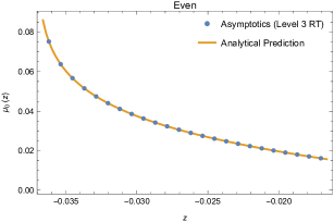
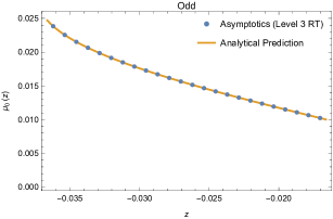
Figure 2: The continuous line is the expected value (4.23) for the coefficient $\mu_{0}$, as a function of $z$, while the dots are numerical approximations based on extrapolation and acceleration of the appropriate auxiliary sequence. The figure on the left corresponds to even values of $\chi$, while the figure on the right corresponds to odd values.

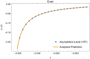
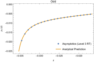
Figure 3: The continuous line is the expected value (4.24) for the coefficient $\mu_{1}$, as a function of $z$, while the dots are numerical approximations based on extrapolation and acceleration of the appropriate auxiliary sequence. The figure on the left corresponds to even values of $\chi$, while the figure on the right corresponds to odd values.

5 Conclusions

In this paper we have initiated the study of the resurgent structure of Walcher’s real topological string. By generalizing the ideas of cesv1 ; cesv2 and the operator formalism of gm-multi ; gkkm , we have obtained multi-instanton amplitudes of the real topological string as trans-series solutions of Walcher’s HAE. The resulting resurgent structure is slightly more complicated than in the closed string case, since the boundary conditions coming from the large radius and the conifold behavior lead to different trans-series. However, as in the closed string case, the multi-instanton amplitudes are essentially obtained by an integer shift of the closed string background, while the D-brane and orientifold background is unaffected.

We find it remarkable that the operator formalism of gm-multi ; gkkm can be extended naturally to the real case. The underlying reason might be that, as shown in ooguri-real ; nw , one can relate the solutions of Walcher’s extended HAE, to solutions of the HAE of bcov for the closed topological string. Perhaps the observations of ooguri-real ; nw lead to a simpler derivation of the operator formalism obtained in this paper.

The full resurgent structure of the real topological string involves additional Stokes constants, as compared to the closed string case. It is natural to conjecture that the new Stokes constants are related to the counting of BPS states in the presence of D-branes and orientifold planes. Concrete evidence for this connection has been obtained in section 3.5, where we found that the integer invariants counting disks indeed appear as Stokes constants in the resurgent structure. More generally, our results indicate that the theory of Donaldson–Thomas invariants underlying BPS counting has a natural extension to the real case. It would be very interesting to develop these observations further, and to find a wall-crossing interpretation for the new Stokes automorphism formula (3.138), in the spirit of KS . Another interesting direction is the study of the real topological string on compact CYs from the point of view of resurgence. In this endeavour, a better understanding of the free energies at high Euler characteristic would be very useful, and it is clearly an interesting problem in itself.

Acknowledgements

We would like to thank Johannes Walcher for his insightful comments on a preliminary draft of this paper. This work has been supported in part by the ERC-SyG project “Recursive and Exact New Quantum Theory” (ReNewQuantum), which received funding from the European Research Council (ERC) under the European Union’s Horizon 2020 research and innovation program, grant agreement No. 810573.

Appendix A Local ${\mathbb{P}}^{2}$

A.1 Useful formulae

In this section we collect some explicit formulae for the special geometry of local ${\mathbb{P}}^{2}$ which can be found in e.g. hkr ; cesv2 ; coms .

The periods solve the Picard–Fuchs equation $\mathfrak{L}\varphi(z)=0$, where

$$\mathfrak{L}=\theta_{z}^{3}+3z\theta_{z}(3\theta_{z}+1)(3\theta_{z}+2)$$ (A.1)

and $\theta_{z}=z{\rm d}/{\rm d}z$. They are built from the power series

$$\widetilde{\varpi}_{1}(z) =\sum_{j\geq 1}3{(3j-1)!\over(j!)^{3}}(-z)^{j},$$ (A.2)

$$\widetilde{\varpi}_{2}(z) =\sum_{j\geq 1}{18\over j!}{\Gamma(3j)\over\Gamma(1+j)^{2}}\left\{\psi(3j)-\psi(j+1)\right\}(-z)^{j},$$

so that

$$t=-\log(z)-\widetilde{\varpi}_{1}(z).$$ (A.3)

The prepotential $F_{0}(t)$ is defined by

$$\partial_{t}F_{0}(t)={\omega_{2}(z)\over 6},$$ (A.4)

where

$$\omega_{2}(z)=\log^{2}(z)+2\widetilde{\varpi}_{1}(z)\log(z)+\widetilde{\varpi}_{2}(z).$$ (A.5)

The conifold discriminant is

$$\delta=1+27z.$$ (A.6)

The Yukawa coupling is given by

$$C_{z}=-{1\over 3z^{3}\delta(z)},$$ (A.7)

The flat coordinate at the conifold is

$$t_{c}(z)={\mathfrak{c}\over 6}\left(\omega_{c}(z)-\pi^{2}\right),\qquad\mathfrak{c}={3\over 2\pi}$$ (A.8)

where

$$\omega_{c}(z)=\log^{2}(-z)+2\log(-z)\widetilde{\varpi}_{1}(z)+\widetilde{\varpi}_{2}(z).$$ (A.9)

It has the property that

$$t_{c}\left(-{1\over 27}\right)=0.$$ (A.10)

Let us note that

$$\omega_{c}(z)=\omega_{2}(z)\pm 2\pi{\rm i}\omega_{1}(z)-\pi^{2},$$ (A.11)

where the sign reflects the choice of branch for $\log(z)$. The expressions (A.8) and (A.9) define $t_{c}(z)$ inside the region of convergence of the series $\widetilde{\varpi}_{1,2}(z)$. Outside this region, it is convenient to use an expression for $t_{c}$ in terms of a Meijer function:

$$t_{c}(z)={3\over 2\pi}\left({\cal G}(-z)-{\pi^{2}\over 6}\right),$$ (A.12)

where

$${\cal G}(z)=\frac{G_{3,3}^{3,2}\left(27z\left|\begin{array}[]{c}\frac{1}{3},\frac{2}{3},1\\ 0,0,0\\ \end{array}\right.\right)}{2\sqrt{3}\pi}-\frac{5\pi^{2}}{18}.$$ (A.13)

Another useful expression is cesv2 ; cms

$$t_{c}(z)=\frac{2\pi}{3}\left(\frac{3\psi}{\Gamma\left(\frac{2}{3}\right)^{3}}\,\,{}_{3}F_{2}\left.\left(\frac{1}{3},\frac{1}{3},\frac{1}{3};\frac{2}{3},\frac{4}{3}\,\right|\psi^{3}\right)-\frac{9\,\psi^{2}}{2\Gamma\left(\frac{1}{3}\right)^{3}}\,\,{}_{3}F_{2}\left.\left(\frac{2}{3},\frac{2}{3},\frac{2}{3};\frac{4}{3},\frac{5}{3}\,\right|\psi^{3}\right)-1\right),$$ (A.14)

where

$$\psi^{3}=-{1\over 27z}.$$ (A.15)

This flat coordinate has the following power series expansion near the conifold point,

$$t_{c}(z)=\frac{1}{\sqrt{3}}\delta+{11\over 18\sqrt{3}}\delta^{2}+{109\over 243\sqrt{3}}\delta^{3}+\cdots$$ (A.16)

A.2 An integral representation of the domain wall tension

It was pointed out in walcher-tadpole that the domain wall tension for local ${\mathbb{P}}^{2}$ (4.1) can be obtained as a definite integral of the canonical Liouville one-form on the mirror curve. This is the local version of the general approach of walcher-dq ; walcher-bcov ; mwalcher to domain wall tensions. Since this is not fully developed in walcher-tadpole , we provide here some details for completeness.

The mirror curve of local ${\mathbb{P}}^{2}$ is given by

$${\rm e}^{x}+{\rm e}^{y}+{\rm e}^{-y-x}+\kappa=0,$$ (A.17)

where $\kappa^{3}=z^{-1}$ and $z$ is the modulus of local ${\mathbb{P}}^{2}$. It is useful to consider the exponentiated variables

$$X={\rm e}^{x},\qquad Y={\rm e}^{y}.$$ (A.18)

We note that the equation for the curve can be solved as

$$Y={X^{2}+\kappa X+{\sqrt{(X^{2}+\kappa X)^{2}-4X}}\over 2X}.$$ (A.19)

Let us consider the points $p=(X,Y)$ in exponentiated variables given by

$$p_{\pm}=\pm\left(\kappa^{-1/2},-\kappa^{-1/2}\right),$$ (A.20)

which belong to the curve (A.17). Then, we have that

$${1\over\xi}{\cal T}(z)=\int_{X_{-}}^{X_{+}}\log(Y){{\rm d}X\over X}.$$ (A.21)

To verify this, we expand in series around $z=0$, to make contact with the expression (4.1). The expansion of $y$ reads

$$\log(Y)=-{1\over 3}\log(z)+\sum_{n\geq 1}z^{n/2}p_{n}(u),$$ (A.22)

where we have introduced the variable $u$ through $X=\kappa^{-1/2}u$, and $p_{n}(u)$ are Laurent polynomials in $u$. One has, for example,

$$p_{1}(u)=u-u^{-1},\qquad p_{2}(u)=-\frac{u^{2}}{2}-\frac{3}{2u^{2}}+2.$$ (A.23)

One also notes that $p_{n}(u)$ are even (odd) functions of $u$ for $n$ even (odd). To perform the integral (A.21) we have to be careful, since the integrand is singular at $u=0$. We just consider the indefinite integral

$$\int^{u}p_{n}(u^{\prime}){{\rm d}u^{\prime}\over u^{\prime}}=P_{n}(u),$$ (A.24)

and we declare

$${1\over\xi}{\cal T}(z)=\int_{-1}^{1}\log(Y){{\rm d}u\over u}=2\sum_{k\geq 0}z^{k+1/2}P_{2k+1}(1),$$ (A.25)

so that only the integrals of odd terms in the series contribute. Then, one verifies that the expansion (4.1) is recovered, as claimed in walcher-tadpole .

References

- (1) D. J. Gross and V. Periwal, String Perturbation Theory Diverges, Phys. Rev. Lett. 60 (1988) 2105.
- (2) S. H. Shenker, The Strength of nonperturbative effects in string theory, in Cargese Study Institute: Random Surfaces, Quantum Gravity and Strings Cargese, France, May 27-June 2, 1990, pp. 191–200, 1990.
- (3) M. Mariño, Lectures on non-perturbative effects in large gauge theories, matrix models and strings, Fortsch. Phys. 62 (2014) 455–540, [1206.6272].
- (4) J. Polchinski, Combinatorics of boundaries in string theory, Phys. Rev. D 50 (1994) R6041–R6045, [hep-th/9407031].
- (5) M. Mariño, Open string amplitudes and large order behavior in topological string theory, JHEP 0803 (2008) 060, [hep-th/0612127].
- (6) M. Mariño, R. Schiappa and M. Weiss, Nonperturbative effects and the large-order behavior of matrix models and topological strings, Commun. Num. Theor. Phys. 2 (2008) 349–419, [0711.1954].
- (7) M. Mariño, Nonperturbative effects and nonperturbative definitions in matrix models and topological strings, JHEP 0812 (2008) 114, [0805.3033].
- (8) T. M. Seara and D. Sauzin, Resumació de Borel i teoria de la ressurgencia, Butl. Soc. Catalana Mat. 18 (2003) 131–153.
- (9) C. Mitschi and D. Sauzin, Divergent series, summability and resurgence. I, vol. 2153 of Lecture Notes in Mathematics. Springer, 2016, 10.1007/978-3-319-28736-2.
- (10) I. Aniceto, G. Başar and R. Schiappa, A primer on resurgent transseries and their asymptotics, Phys. Rep. 809 (2019) 1–135.
- (11) M. Mariño, Instantons and large . An introduction to non-perturbative methods in quantum field theory. Cambridge University Press, 2015.
- (12) J. Gu and M. Mariño, Peacock patterns and new integer invariants in topological string theory, SciPost Phys. 12 (2022) 058, [2104.07437].
- (13) M. Alim, A. Saha, J. Teschner and I. Tulli, Mathematical Structures of Non-perturbative Topological String Theory: From GW to DT Invariants, Commun. Math. Phys. 399 (2023) 1039–1101, [2109.06878].
- (14) A. Grassi, Q. Hao and A. Neitzke, Exponential Networks, WKB and Topological String, SIGMA 19 (2023) 064, [2201.11594].
- (15) J. Gu and M. Mariño, Exact multi-instantons in topological string theory, 2211.01403.
- (16) C. Rella, Resurgence, Stokes constants, and arithmetic functions in topological string theory, 2212.10606.
- (17) J. Gu, A.-K. Kashani-Poor, A. Klemm and M. Mariño, Non-perturbative topological string theory on compact Calabi-Yau 3-folds, 2305.19916.
- (18) J. Gu, Relations between Stokes constants of unrefined and Nekrasov-Shatashvili topological strings, 2307.02079.
- (19) K. Iwaki and M. Mariño, Resurgent Structure of the Topological String and the First Painlevé Equation, 2307.02080.
- (20) S. Gukov, M. Mariño and P. Putrov, Resurgence in complex Chern-Simons theory, 1605.07615.
- (21) S. Garoufalidis, J. Gu and M. Mariño, The Resurgent Structure of Quantum Knot Invariants, Commun. Math. Phys. 386 (2021) 469–493, [2007.10190].
- (22) S. Garoufalidis, J. Gu and M. Mariño, Peacock patterns and resurgence in complex Chern–Simons theory, Research in the Mathematical Sciences 10 (2023) 29, [2012.00062].
- (23) S. Garoufalidis, J. Gu, M. Mariño and C. Wheeler, Resurgence of Chern-Simons theory at the trivial flat connection, 2111.04763.
- (24) C. Wheeler, Quantum modularity for a closed hyperbolic 3-manifold, 2308.03265.
- (25) M. Bershadsky, S. Cecotti, H. Ooguri and C. Vafa, Holomorphic anomalies in topological field theories, Nucl.Phys. B405 (1993) 279–304, [hep-th/9302103].
- (26) M. Bershadsky, S. Cecotti, H. Ooguri and C. Vafa, Kodaira–Spencer theory of gravity and exact results for quantum string amplitudes, Commun. Math. Phys. 165 (1994) 311–428, [hep-th/9309140].
- (27) R. Couso-Santamaría, J. D. Edelstein, R. Schiappa and M. Vonk, Resurgent transseries and the holomorphic anomaly, Annales Henri Poincaré 17 (2016) 331–399, [1308.1695].
- (28) R. Couso-Santamaría, J. D. Edelstein, R. Schiappa and M. Vonk, Resurgent transseries and the holomorphic anomaly: Nonperturbative closed strings in local , Commun. Math. Phys. 338 (2015) 285–346, [1407.4821].
- (29) S. Codesido, M. Mariño and R. Schiappa, Non-Perturbative Quantum Mechanics from Non-Perturbative Strings, Annales Henri Poincare 20 (2019) 543–603, [1712.02603].
- (30) S. Codesido, A geometric approach to non-perturbative quantum mechanics. PhD thesis, University of Geneva, 2018.
- (31) F. David, Nonperturbative effects in matrix models and vacua of two-dimensional gravity, Phys. Lett. B 302 (1993) 403–410, [hep-th/9212106].
- (32) M. Mariño, R. Schiappa and M. Weiss, Multi-Instantons and Multi-Cuts, J.Math.Phys. 50 (2009) 052301, [0809.2619].
- (33) J. Walcher, Opening mirror symmetry on the quintic, Commun. Math. Phys. 276 (2007) 671–689, [hep-th/0605162].
- (34) J. Walcher, Extended holomorphic anomaly and loop amplitudes in open topological string, Nucl. Phys. B 817 (2009) 167–207, [0705.4098].
- (35) J. Walcher, Evidence for Tadpole Cancellation in the Topological String, Commun. Num. Theor. Phys. 3 (2009) 111–172, [0712.2775].
- (36) D. Krefl and J. Walcher, The Real Topological String on a local Calabi-Yau, 0902.0616.
- (37) P. Candelas, X. C. De La Ossa, P. S. Green and L. Parkes, A Pair of Calabi-Yau manifolds as an exactly soluble superconformal theory, Nucl. Phys. B 359 (1991) 21–74.
- (38) R. Gopakumar and C. Vafa, M-theory and topological strings. 2., hep-th/9812127.
- (39) M. Dedushenko and E. Witten, Some Details On The Gopakumar-Vafa and Ooguri-Vafa Formulas, Adv. Theor. Math. Phys. 20 (2016) 1–133, [1411.7108].
- (40) D. Krefl and J. Walcher, Extended holomorphic anomaly in gauge theory, Lett. Math. Phys. 95 (2011) 67–88, [1007.0263].
- (41) N. Piazzalunga and A. M. Uranga, M-theory interpretation of the real topological string, JHEP 08 (2014) 054, [1405.6019].
- (42) P. Candelas and X. de la Ossa, Moduli Space of Calabi-Yau Manifolds, Nucl. Phys. B 355 (1991) 455–481.
- (43) A. Klemm, The B-model approach to topological string theory on Calabi-Yau -folds, in B-model Gromov-Witten theory (E. Clader and Y. Ruan, eds.), Springer–Verlag, 2018.
- (44) S. Yamaguchi and S.-T. Yau, Topological string partition functions as polynomials, JHEP 07 (2004) 047, [hep-th/0406078].
- (45) M.-x. Huang and A. Klemm, Holomorphic anomaly in gauge theories and matrix models, JHEP 09 (2007) 054, [hep-th/0605195].
- (46) T. W. Grimm, A. Klemm, M. Mariño and M. Weiss, Direct integration of the topological string, JHEP 08 (2007) 058, [hep-th/0702187].
- (47) M. Alim and J. D. Lange, Polynomial Structure of the (Open) Topological String Partition Function, JHEP 10 (2007) 045, [0708.2886].
- (48) S. Hosono, BCOV ring and holomorphic anomaly equation, Adv. Stud. Pure Math. 59 (2008) 79, [0810.4795].
- (49) A. Neitzke and J. Walcher, Background independence and the open topological string wavefunction, Proc. Symp. Pure Math. 78 (2008) 285, [0709.2390].
- (50) D. Ghoshal and C. Vafa, string as the topological theory of the conifold, Nucl. Phys. B 453 (1995) 121–128, [hep-th/9506122].
- (51) B. Haghighat, A. Klemm and M. Rauch, Integrability of the holomorphic anomaly equations, JHEP 0810 (2008) 097, [0809.1674].
- (52) R. Couso-Santamaría, M. Mariño and R. Schiappa, Resurgence matches quantization, J. Phys. A50 (2017) 145402, [1610.06782].
- (53) A. Klemm and E. Zaslow, Local mirror symmetry at higher genus, hep-th/9906046.
- (54) S. Garoufalidis, A. Its, A. Kapaev and M. Mariño, Asymptotics of the instantons of Painlevé I, Int. Math. Res. Not. 2012 (2012) 561–606, [1002.3634].
- (55) I. Aniceto, R. Schiappa and M. Vonk, The resurgence of instantons in string theory, Commun. Num. Theor. Phys. 6 (2012) 339–496, [1106.5922].
- (56) M. Mariño, R. Schiappa and M. Schwick, New Instantons for Matrix Models, 2210.13479.
- (57) S. Pasquetti and R. Schiappa, Borel and Stokes nonperturbative phenomena in topological string theory and matrix models, Annales Henri Poincaré 11 (2010) 351–431, [0907.4082].
- (58) S. Alexandrov and B. Pioline, Theta series, wall-crossing and quantum dilogarithm identities, Lett. Math. Phys. 106 (2016) 1037–1066, [1511.02892].
- (59) I. Coman, P. Longhi and J. Teschner, From quantum curves to topological string partition functions II, 2004.04585.
- (60) M. Aganagic and C. Vafa, Mirror symmetry, D-branes and counting holomorphic discs, hep-th/0012041.
- (61) M. Aganagic, A. Klemm and C. Vafa, Disk instantons, mirror symmetry and the duality web, Z.Naturforsch. A57 (2002) 1–28, [hep-th/0105045].
- (62) F. Villegas, Modular Mahler Measures I, Topics in Number Theory, vol. 467 of Mathematics and Its Applications, pp. 17–48. Springer US, 1999.
- (63) C. F. Doran and M. Kerr, Algebraic K-theory of toric hypersurfaces, Commun. Number Theory Phys. 5 (2011) 397–600, [0809.4669].
- (64) M. Mariño and S. Zakany, Matrix models from operators and topological strings, Annales Henri Poincaré 17 (2016) 1075–1108, [1502.02958].
- (65) K. Bönisch, A. Klemm, E. Scheidegger and D. Zagier, D-brane masses at special fibres of hypergeometric families of Calabi-Yau threefolds, modular forms, and periods, 2203.09426.
- (66) D. Krefl, S. Pasquetti and J. Walcher, The Real Topological Vertex at Work, Nucl. Phys. B 833 (2010) 153–198, [0909.1324].
- (67) P. L. H. Cook, H. Ooguri and J. Yang, Comments on the Holomorphic Anomaly in Open Topological String Theory, Phys. Lett. B 653 (2007) 335–337, [0706.0511].
- (68) M. Kontsevich and Y. Soibelman, Stability structures, motivic Donaldson-Thomas invariants and cluster transformations, 0811.2435.
- (69) D. R. Morrison and J. Walcher, D-branes and Normal Functions, Adv. Theor. Math. Phys. 13 (2009) 553–598, [0709.4028].