Gravitational Wave imprints of the
Doublet Left-Right Symmetric Model

Abstract

We study the gravitational wave (GW) signature in the doublet left-right symmetric model (DLRSM) resulting from the strong first-order phase transition (SFOPT) associated with $SU(2)_{R}\times U(1)_{B-L}$-breaking. For different values of the symmetry-breaking scale $v_{R}=20,~{}30$, and $50$ TeV, we construct the one-loop finite temperature effective potential to explore the parameter space for regions showing SFOPT. We identify the region where the associated stochastic GW background is strong enough to be detected at planned GW observatories. A strong GW background favors a relatively light CP-even neutral scalar $H_{3}$, arising from the $SU(2)_{R}$ doublet. The $SU(2)_{L}$ subgroup of DLRSM is broken by three vevs: $\kappa_{1},~{}\kappa_{2}$, and $v_{L}$. We also observe a preference for $\mathcal{O}(1)$ values of the ratio $w=v_{L}/\kappa_{1}$, but no clear preference for the ratio $r=\kappa_{2}/\kappa_{1}$. A large number of points with strong GW signal can be ruled out from precise measurement of the trilinear Higgs coupling and searches for $H_{3}$ at the future colliders.

I Introduction

The left-right symmetric model (LRSM) Pati:1974yy ; Mohapatra:1974gc ; PhysRevD.11.566 ; Senjanovic:1975rk ; Senjanovic:1978ev is an attractive extension that addresses several limitations of the standard model (SM). In LRSM, the SM gauge group is extended from $\mathcal{G}_{\rm{SM}}=SU(3)_{c}\times SU(2)_{L}\times U(1)_{Y}$ to $\mathcal{G}_{\rm{LRSM}}=SU(3)_{c}\times SU(2)_{L}\times SU(2)_{R}\times U(1)_{B-L}$ and the right-chiral fermions transform as doublets under the $SU(2)_{R}$ subgroup. There are different realizations of LRSM, depending on the scalars involved in the spontaneous breaking of $\mathcal{G}_{\textrm{LRSM}}$ to $\mathcal{G}_{\rm{SM}}$. These also differ in the mechanism for generating fermion masses. The triplet left-right symmetric model (TLRSM) Maiezza:2016ybz ; PhysRevD.44.837 ; Senjanovic:2016bya , contains a scalar bi-doublet, and two $SU(2)$ triplets. The charged fermion masses are then generated by the bi-doublet, whereas the neutrino masses are generated by the type-II seesaw mechanism. On the other hand, the scalar sector of a doublet left-right symmetric model (DLRSM) consists of a scalar bi-doublet and a pair of $SU(2)$ doublets Senjanovic:1978ev ; Mohapatra:1977be . In DLRSM, neutrino masses can be incorporated by extending the model with an additional charged singlet scalar Babu:1988qv ; FileviezPerez:2016erl ; FileviezPerez:2017zwm ; Babu:2020bgz . Apart from TLRSM and DLRSM, other variations have also been discussed in the literature and have different experimental consequences Ma:2012gb ; Frank:2020odd ; Graf:2021xku .

The observation of gravitational waves (GW) from a binary black hole merger by the aLIGO collaboration in 2015 Abbott_2016 was a landmark discovery that marked the beginning of the era of GW astronomy. At present, two facilities of the LIGO collaboration Harry:2010zz and one facility of the VIRGO collaboration VIRGO:2012dcp are functional. Several other ground-based and space-based observatories such as LISA LISA:2017pwj , DECIGO Seto:2001qf , BBO Corbin:2005ny , ET Punturo:2010zz , and CE LIGOScientific:2016wof are planned and will be functional in the coming decades. It has long been known that phenomena in the early universe such as inflation, cosmic strings, domain walls, and strong first-order phase transitions (SFOPT) can lead to a stochastic GW background Caprini:2015zlo ; Athron:2023xlk ; LISACosmologyWorkingGroup:2022jok ; Caprini:2018mtu . The upcoming GW observatories will be capable of detecting the GW background from SFOPT up to symmetry-breaking scales as high as $10^{6}-10^{7}$ GeV Dev:2016feu ; Addazi:2018nzm ; Ringe:2022rjx , making GW astronomy an important tool to test beyond standard model (BSM) theories.

In this paper, we study the GW production associated with SFOPT in DLRSM. Since a right-handed charged current has not been observed at colliders so far, the $SU(2)_{R}\times U(1)_{B-L}$ subgroup of DLRSM must be broken at a scale, $v_{R}$, much higher than the electroweak (EW) scale. This puts a lower bound, $v_{R}\gtrsim\mathcal{O}(10)$ TeV, but there is no upper bound as such. GW astronomy presents a novel approach to probe the scale $v_{R}$ by studying the possibility of an observable GW background from SFOPT within the LRSM. Different realizations of LRSM have been explored in the literature for GW imprints: through SFOPT in TRLSM Brdar:2019fur ; Li:2020eun and a minimal LR model with seesaw-like fermion mass generation Graf:2021xku , and also from domain walls arising out of the breaking of the discrete parity symmetry Borah:2022wdy .

In DLRSM (TLRSM), electroweak symmetry breaking (EWSB) happens via three vevs : $\kappa_{1},~{}\kappa_{2}$, coming from the bi-doublet, and $v_{L}$ coming from the $SU(2)_{L}$ doublet (triplet). These are constrained by the relation, $\kappa_{1}^{2}+\kappa_{2}^{2}+v_{L}^{2}=v^{2}$, where $v=246$ GeV. It is useful to define the vev ratios: $r=\kappa_{2}/\kappa_{1},~{}w=v_{L}/\kappa_{1}$. Contrary to TLRSM, there are no sources of custodial symmetry breaking in DLRSM at the tree level. Hence the vevs $\kappa_{1},~{}\kappa_{2}$, and $v_{L}$ can all be sizable, i.e. $r$ and $w$ can be $\mathcal{O}(0.1)$ and $\mathcal{O}(1)$ respectively. In fact, it was shown in ref. Bernard:2020cyi , that the EW precision data prefers a large value of $w$. In ref. Karmakar:2022iip it was further shown that the measurement of the Higgs signal strength and meson mixing bounds prefer large values of $r$ and $w$. It is therefore interesting to note that, unlike TLRSM, EWSB in DLRSM can be considerably different from that in SM, even though the $SU(2)_{R}\times U(1)_{B-L}$-breaking dynamics is decoupled from the EW scale. In this paper, we ask (i) whether DLRSM can lead to a detectable GW background in some region of the parameter space, and (ii) whether this region of the parameter space prefers a special pattern of EWSB.

In Sec. II, we give a brief review of DLRSM: field content, symmetry breaking, and mass generation in the gauge, fermion, and gauge sectors. In Sec. II.4 and Sec. II.5, we discuss the theoretical bounds and the constraints from the Higgs data respectively. In Sec. III, we construct the one-loop finite temperature effective potential required to study the phase transition (PT) associated with $SU(2)_{R}\times U(1)_{B-L}$-breaking. The separation between $v_{R}$ and the EW scale allows us to write the effective potential only in terms of the field responsible $SU(2)_{R}\times U(1)_{B-L}$-breaking. We then describe our procedure for scanning the parameter space in Sec. IV. To simplify the analysis while extracting crucial information related to SFOPT, we work with a smaller set of parameters, called the simple basis, introduced in ref. Karmakar:2022iip . In the simple basis, we identify the region with SFOPT. Next, in Sec. V, we discuss the GW background obtained for points with SFOPT. In Sec. VI, we compute the signal-to-noise ratio (SNR) for six benchmark points, at various planned GW detectors such as FP-DECIGO, BBO, and Ultimate-DECIGO. In Sec. VII, we discuss future collider probes that can complement the GW signal. Finally, in Sec. VIII, we summarize our key findings and present concluding remarks.

II The model

We follow the notation of refs. Bernard:2020cyi ; Karmakar:2022iip for the scalar potential and vev structure of the scalar multiplets. The fermion content of the model has the following charges under the LRSM gauge group, $\mathcal{G}_{\rm{LRSM}}=SU(3)_{c}\times SU(2)_{L}\times SU(2)_{R}\times U(1)_{B-L}$,

$$Q_{L} = \begin{pmatrix}u_{L}\\ d_{L}\end{pmatrix}\sim(3,2,1,1/3),\hskip 28.45274ptQ_{R}=\begin{pmatrix}u_{R}\\ d_{R}\end{pmatrix}\sim(3,1,2,1/3),$$

$$L_{L} = \begin{pmatrix}\nu_{L}\\ e_{L}\end{pmatrix}\sim(1,2,1,-1),\hskip 34.1433ptL_{R}=\begin{pmatrix}\nu_{R}\\ e_{R}\end{pmatrix}\sim(1,1,2,-1),$$ (1)

where the quantum numbers of the multiplets under the sub-groups of $\mathcal{G}_{\rm{LRSM}}$ are indicated in brackets. We have suppressed the family index $i\in\{1,2,3\}$ for three generations of quarks and three generations of leptons.The right-handed neutrino $\nu_{R}$ is needed to complete the $SU(2)_{R}$ lepton doublet. This choice of fermions is required for the cancellation of the $U(1)_{B-L}$ gauge anomaly and ensures that the model is manifestly symmetric under the transformations: $Q_{L}\leftrightarrow Q_{R}$, $L_{L}\leftrightarrow L_{R}$.

II.1 Scalar sector

The scalar sector of DLRSM includes a complex bi-doublet $\Phi$ needed to generate charged fermion masses, and two doublets $\chi_{L}$ and $\chi_{R}$, which participate in the EW- and LR-symmetry breaking respectively. These scalar multiplets and their charges under $\mathcal{G}_{\text{LRSM}}$ are:

$$\Phi=\begin{pmatrix}\phi_{1}^{0}&\phi_{2}^{+}\\ \phi_{1}^{-}&\phi_{2}^{0}\end{pmatrix}\sim(1,2,2,0),~{}\chi_{L}=\begin{pmatrix}\chi_{L}^{+}\\ \chi_{L}^{0}\end{pmatrix}\sim(1,2,1,1),~{}\text{and}~{}\chi_{R}=\begin{pmatrix}\chi_{R}^{+}\\ \chi_{R}^{0}\end{pmatrix}\sim(1,1,2,1).$$

We take the potential to be parity-symmetric, i.e. the couplings of ‘L’ and ‘R’ fields are equal. The most general, CP-conserving, renormalizable scalar potential is then given by,

$$V = V_{2}+V_{3}+V_{4},$$

$$V_{2} = -\mu_{1}^{2}{\rm{Tr}}(\Phi^{\dagger}\Phi)-\mu_{2}^{2}\ [{\rm{Tr}}(\tilde{\Phi}\Phi^{\dagger})+{\rm{Tr}}(\tilde{\Phi}^{\dagger}\Phi)]-\mu_{3}^{2}\ [\chi_{L}^{\dagger}\chi_{L}+\chi_{R}^{\dagger}\chi_{R}],$$

$$V_{3} = \mu_{4}\ [\chi_{L}^{\dagger}\Phi\chi_{R}+\chi_{R}^{\dagger}\Phi^{\dagger}\chi_{L}]+\mu_{5}\ [\chi_{L}^{\dagger}\tilde{\Phi}\chi_{R}+\chi_{R}^{\dagger}\tilde{\Phi}^{\dagger}\chi_{L}],$$

$$V_{4} = \lambda_{1}{\rm{Tr}}(\Phi^{\dagger}\Phi)^{2}+\lambda_{2}\ [{\rm{Tr}}(\tilde{\Phi}\Phi^{\dagger})^{2}+{\rm{Tr}}(\tilde{\Phi}^{\dagger}\Phi)^{2}]+\lambda_{3}\text{Tr}(\tilde{\Phi}\Phi^{\dagger})\,{\rm{Tr}}(\tilde{\Phi}^{\dagger}\Phi)$$ (3)

$$+\lambda_{4}{\rm{Tr}}(\Phi^{\dagger}\Phi)\,[{\rm{Tr}}(\tilde{\Phi}\Phi^{\dagger})+{\rm{Tr}}(\tilde{\Phi}^{\dagger}\Phi)]+\rho_{1}\ [(\chi_{L}^{\dagger}\chi_{L})^{2}+(\chi_{R}^{\dagger}\chi_{R})^{2}]+\rho_{2}\ \chi_{L}^{\dagger}\chi_{L}\chi_{R}^{\dagger}\chi_{R}$$

$$+\alpha_{1}{\rm{Tr}}(\Phi^{\dagger}\Phi)[\chi_{L}^{\dagger}\chi_{L}+\chi_{R}^{\dagger}\chi_{R}]+\Big{\{}\alpha_{2}\ [\chi_{L}^{\dagger}\chi_{L}{\rm{Tr}}(\tilde{\Phi}\Phi^{\dagger})+\chi_{R}^{\dagger}\chi_{R}{\rm{Tr}}(\tilde{\Phi}^{\dagger}\Phi)]+{\rm h.c.}\Big{\}}$$

$$+\alpha_{3}\ [\chi_{L}^{\dagger}\ \Phi\Phi^{\dagger}\chi_{L}+\chi_{R}^{\dagger}\Phi^{\dagger}\Phi\chi_{R}]+\alpha_{4}\ [\chi_{L}^{\dagger}\ \tilde{\Phi}\tilde{\Phi}^{\dagger}\chi_{L}+\chi_{R}^{\dagger}\tilde{\Phi}^{\dagger}\tilde{\Phi}\chi_{R}],$$

with $\tilde{\Phi}\equiv\sigma_{2}\Phi^{*}\sigma_{2}$. The potential has mass parameters: $\{\mu_{1,2,3,4,5}\}$, and quartic couplings: $\{\lambda_{1,2,3,4},\alpha_{1,2,3,4},\rho_{1,2}\}$. We assume all parameters to be real for simplicity.

The neutral scalars can be written in terms of real and imaginary components,

$$\phi_{1}^{0} = \frac{1}{\sqrt{2}}(\phi_{1r}^{0}+i\phi_{1i}^{0}),\,\,\,\,\phi_{2}^{0}=\frac{1}{\sqrt{2}}(\phi_{2r}^{0}+i\phi_{2i}^{0}),$$

$$\chi_{L}^{0} = \frac{1}{\sqrt{2}}(\chi_{Lr}^{0}+i\chi_{Li}^{0}),\,\,\,\,\chi_{R}^{0}=\frac{1}{\sqrt{2}}(\chi_{Rr}^{0}+i\chi_{Ri}^{0}).$$ (4)

We assign non-zero vevs only to the real components of the neutral scalars and do not consider CP- or charge-breaking minima. The vev structure is denoted by

$$\langle\Phi\rangle=\frac{1}{\sqrt{2}}\begin{pmatrix}\kappa_{1}&0\\ 0&\kappa_{2}\end{pmatrix},~{}\langle\chi_{L}\rangle=\frac{1}{\sqrt{2}}\begin{pmatrix}0\\ v_{L}\end{pmatrix},~{}\langle\chi_{R}\rangle=\frac{1}{\sqrt{2}}\begin{pmatrix}0\\ v_{R}\end{pmatrix}\,.$$ (5)

The pattern of symmetry breaking is as follows:

$$SU(2)_{L}\times SU(2)_{R}\times U(1)_{B-L}\xrightarrow{\mathit{~{}~{}v_{R}~{}~{}}}SU(2)_{L}\times U(1)_{Y}\xrightarrow{\mathit{\kappa_{1},\kappa_{2},v_{L}}}U(1)_{Y}.$$

The vev $v_{R}$ of the doublet $\chi_{R}$ breaks $SU(2)_{R}$, while the three vevs $\kappa_{1},~{}\kappa_{2}$, and $v_{L}$ trigger EWSB. As mentioned earlier, the EW vevs can be conveniently expressed in terms of the vev ratios $r$ and $w$ as, $\kappa_{2}=r\kappa_{1}$ and $v_{L}=w\kappa_{1}$. Then, $\kappa_{1}^{2}(1+r^{2}+w^{2})=v^{2}$, i.e., the value of $\kappa_{1}$ is fixed for a given $r$ and $w$. The absence of a right-handed charged current in collider experiments implies a hierarchy of scales $v_{R}\gg v$.

In terms of the vevs $\kappa_{1},\kappa_{2},v_{L}$, and $v_{R}$, the minimization conditions are,

$$\frac{\partial V}{\partial\kappa_{1}}=\frac{\partial V}{\partial\kappa_{2}}=\frac{\partial V}{\partial v_{L}}=\frac{\partial V}{\partial v_{R}}=0.$$ (6)

Using the minimization conditions, we trade $\mu_{1}^{2}$, $\mu_{2}^{2}$, $\mu_{3}^{2}$, and $\mu_{5}$ for the vevs , $\mu_{4}$, and quartic couplings (see appendix A for full expressions). Thus the parameters of the DLRSM scalar sector reduce to

$$\{\lambda_{1,2,3,4},\alpha_{1,2,3,4},\rho_{1,2},\mu_{4},r,w,v_{R}\}\,\,.$$ (7)

The CP-even, CP-odd, and charged scalar mass matrices are obtained using

$$m^{2}_{ij}=\left.\frac{\partial^{2}V}{\partial\varphi_{i}\,\partial\varphi_{j}}\right|_{\langle\varphi\rangle},$$ (8)

where

$$\varphi\equiv\{\phi^{0}_{1r},\phi^{0}_{2r},\chi^{0}_{Lr},\chi^{0}_{Rr},\phi^{0}_{1i},\phi^{0}_{2i},\chi^{0}_{Li},\chi^{0}_{Ri},\phi^{\pm}_{1},\phi^{\pm}_{2},\chi^{\pm}_{L},\chi^{\pm}_{R}\}\,\,.$$ (9)

Physical scalar masses and mixing angles are obtained by diagonalizing these matrices. We denote the physical spectrum of scalars by: CP-even scalars, $h,~{}H_{1},~{}H_{2},~{}H_{3}$, CP-odd scalars, $A_{1},~{}A_{2}$, and the charged scalars, $H_{1}^{\pm},~{}H_{2}^{\pm}$.

The lightest CP-even scalar, $h$ has a mass of the order $v$, and is identified with the SM-like Higgs with mass $\sim 125$ GeV. Using non-degenerate perturbation theory, $m_{h}$ is estimated as Bernard:2020cyi ; Karmakar:2022iip

$$m_{h,\text{analytic}}^{2} = \frac{\kappa_{1}^{2}}{2(1+r^{2}+w^{2})}\times$$ (10)

$$\Bigg{(}4\Big{(}\lambda_{1}(r^{2}+1)^{2}+4r(\lambda_{4}(r^{2}+1)+r\lambda_{23})+w^{2}(\alpha_{124}+r^{2}(\alpha_{1}+\alpha_{3})$$

$$+\alpha_{2}r)+\rho_{1}w^{4}\Big{)}-\frac{1}{\rho_{1}}(\alpha_{124}+r^{2}(\alpha_{1}+\alpha_{3})+\alpha_{2}r+2\rho_{1}w^{2})^{2}\Bigg{)}\,,$$

where, $\alpha_{124}\equiv\alpha_{1}+r\alpha_{2}+\alpha_{4}$, and $\lambda_{23}=2\lambda_{2}+\lambda_{3}$. In the limit $r,w\rightarrow 0$, the above expression simplifies to

$$m_{h,\text{analytic}}^{2}=v^{2}\left(2\lambda_{1}-\frac{(\alpha_{1}+\alpha_{4})^{2}}{2\rho_{1}}\right).$$ (11)

However, it was pointed out in ref. Karmakar:2022iip that for certain values of the quartic parameters, the analytical estimate for $m_{h}$ may not suffice.

The other scalars have masses of the order $v_{R}$. To $\mathcal{O}\big{(}\kappa_{1}/v_{R}\big{)}$, these masses are related to each other as

$$m_{H_{1}}^{2}\simeq m_{A_{1}}^{2}\simeq m_{H^{\pm}_{1}}^{2}\approx\frac{1}{2}(\alpha_{3}-\alpha_{4})v_{R}^{2}\,,$$

$$m_{H_{2}}^{2}\simeq m_{A_{2}}^{2}\simeq m_{H^{\pm}_{2}}^{2}\approx\frac{1}{2}(\rho_{2}-2\rho_{1})v_{R}^{2}\,,$$

$$m_{H_{3}}^{2}=2\rho_{1}v_{R}^{2}\,,$$

$$m_{H_{2}}^{2}>m_{H_{1}}^{2}\,.$$

The first two mass expressions are valid in the limit $r,w\rightarrow 0$. Positive-definite nature of the CP-even mass matrix leads to two approximate criteria: $\rho_{2}>2\rho_{1}$ and $\alpha_{3}>\alpha_{4}$. In our analysis, we calculate the scalar masses and mixing numerically. The full analytic expressions at the leading order can be found in the appendix of ref. Karmakar:2022iip .

For the CP-even scalars, the mass-squared matrix is diagonalized by the orthogonal matrix $O$,

$$O^{T}\mathcal{M}^{2}_{\text{CPE}}O=\big{(}\mathcal{M}^{\text{diag}}_{\text{CPE}}\big{)}^{2},\,\,\,\,\,\,X_{\text{physical}}=O^{T}X\,,$$ (12)

where $X=(\phi_{1r}^{0},\phi^{0}_{2r},\chi^{0}_{Lr},\chi_{Rr}^{0})^{T}$, $X_{\text{physical}}=(h,H_{1},H_{2},H_{3})^{T}$. The scalars $H_{1}$ and $A_{1}$ can contribute to the mixing of $K_{0}-\bar{K}_{0}$ system, leading to the constraint, $m_{H_{1},A_{1}}>15$ TeV  Zhang:2007da . The scalar $H_{3}$ predominantly originates from the doublet $\chi_{R}$ and its coupling to the SM particles is dominated by the element $O_{41}\sim v^{2}/v_{R}^{2}$. So, it can be much lighter than $H_{1}$.

The triple Higgs $(h^{3})$ coupling in DLRSM is given by Karmakar:2022iip

$$c_{h^{3}} = \frac{\kappa_{1}}{2}\Big{(}2(\lambda_{1}+r\lambda_{4})O_{11}^{3}+2(r\lambda_{1}+\lambda_{4})O_{21}^{3}+2w\rho_{1}O_{31}^{3}+2(r(\lambda_{1}+4\lambda_{2}+2\lambda_{3})+3\lambda_{4})O_{11}^{2}O_{21}$$ (13)

$$\hskip 20.0pt+2(\lambda_{1}+4\lambda_{2}+2\lambda_{3}+3\lambda_{4}r)O_{11}O_{21}^{2}+w(\alpha_{1}+\alpha_{4})O_{11}^{2}O_{31}+(\alpha_{1}+r\alpha_{2}+\alpha_{4})O_{11}O_{31}^{2}$$

$$\hskip 20.0pt+w(\alpha_{1}+\alpha_{3})O_{21}^{2}O_{31}+(\alpha_{2}+r(\alpha_{1}+\alpha_{3}))O_{21}O_{31}^{2}\Big{)}\,\,\,,$$

with the corresponding coupling multiplier $\kappa_{h}=c_{h^{3}}/c_{h^{3}}^{\textrm{SM}}$, where $c_{h^{3}}^{\textrm{SM}}=m_{h}^{2}/2v$.

II.2 Fermion sector

The fermion multiplets couple to the bi-doublet $\Phi$ via Yukawa terms:

$$\mathcal{L}_{\rm{Y}}\supset-\bar{Q}_{Li}(y_{ij}\Phi+\tilde{y}_{ij}\tilde{\Phi})Q_{Rj}+\rm{h.c.}\,\,,$$ (14)

which leads to the mass matrices for the quarks:

$$M_{U}=\frac{1}{\sqrt{2}}(\kappa_{1}y+\kappa_{2}\tilde{y}),\,\,\,\,M_{D}=\frac{1}{\sqrt{2}}(\kappa_{2}y+\kappa_{1}\tilde{y})\,\,,$$

where $M_{U}$ and $M_{D}$ stand for up-type and down-type mass matrices in the flavor basis respectively. To obtain the physical basis of fermions, these mass matrices need to be diagonalized through unitary transformations described by the left- and right-handed CKM matrices ($V_{L,R}^{\textrm{CKM}}$). Manifest left-right symmetry implies $V_{R}^{\textrm{CKM}}=V_{L}^{\textrm{CKM}}$. For the calculation of the effective potential in the next section, it is enough to take $y\approx\text{diag}(0,0,y_{33})$ and $\tilde{y}\approx\text{diag}(0,0,\tilde{y}_{33})$. In the limit $V^{\textrm{CKM}}_{33}\approx 1$,

$$y_{33} = \frac{\sqrt{2}(1+r^{2}+w^{2})^{1/2}}{v(1-r^{2})}(m_{t}-rm_{b}),$$

$$\tilde{y}_{33} = \frac{\sqrt{2}(1+r^{2}+w^{2})^{1/2}}{v(1-r^{2})}(m_{b}-rm_{t}),$$ (15)

where the top and bottom quark masses are $m_{t}=173.5$ GeV, and $m_{b}\approx 5$ GeV. In the limit $r,w\rightarrow 0$, $y_{33}$ and $\tilde{y}_{33}$ reduce to the SM Yukawa couplings $y_{t}$ and $y_{b}$ respectively. However, we do not make any such assumption and use eq. (II.2), allowing $r,w$ to be arbitrary.

The couplings of the SM-like Higgs with the third-generation quarks are given by:

$$c_{htt\,(hbb)}=\frac{\kappa_{1}}{\kappa_{-}^{2}}\,\Big{(}(O_{11}-rO_{21})m_{t(b)}+(O_{21}-rO_{11})(V_{L}^{\text{CKM}}\,\hat{M}_{D(U)}\,V_{R}^{\text{CKM}\dagger})_{33}\Big{)},$$ (16)

where $\kappa^{2}_{-}=\kappa_{1}^{2}-\kappa_{2}^{2}=\kappa_{1}^{2}(1-r^{2})$ and $\hat{M}_{U(D)}$ denotes the diagonal up (down)-type quark mass matrix. Here $O_{ij}$ are the elements of the orthogonal transformation matrix appearing in eq. (12). Then the coupling multipliers, $\kappa_{b}$ and $\kappa_{t}$ are: $\kappa_{f}=c_{hff}/c^{\rm{SM}}_{hff}$, where $c_{hff}^{\rm{SM}}=m_{f}/v$ and $f=t,b$.

Since $V_{L,R}^{\rm{CKM}}\approx\mathbf{1}$, eq. (16), becomes,

$$c_{htt} \approx \frac{\kappa_{1}}{\kappa^{2}_{-}}\big{(}O_{11}(m_{t}-rm_{b})+O_{21}(m_{b}-rm_{t})\big{)},$$

$$c_{hbb} \approx \frac{\kappa_{1}}{\kappa^{2}_{-}}\big{(}O_{11}(m_{b}-rm_{t})+O_{21}(m_{t}-rm_{b})\big{)}$$

Note that there is a hierarchy, $O_{21}\ll O_{11}\sim 1$, $m_{t}\gg m_{b}$, and $r\ll 1$. The SM couplings are recovered by setting $O_{11}=1,O_{21}=0,r=0$, in the above expressions. For a large $\phi_{1r}^{0}-\phi_{2r}^{0}$ mixing, i.e. $O_{21}\gtrsim\mathcal{O}(10^{-2})$ or large $\kappa_{2}$, i.e. $r\sim\mathcal{O}(10^{-1})$, the deviation of $hb\bar{b}$ coupling from the SM value can be quite large due to the multiplicative factors proportional to $O_{21}m_{t}$, and $rO_{11}m_{t}$. On the other hand, the deviation of $ht\bar{t}$ coupling is proportional to $O_{21}m_{b}$ and $rO_{21}m_{t}$, and is therefore rather small for the current precision of $\kappa_{t}$ measurement.

II.3 Gauge sector

In this paper, we work under the assumption of manifest left-right symmetry of the UV-Lagrangian, i.e., $g_{R}=g_{L}=g$. Here, $g_{L(R)}$ are the gauge couplings of $SU(2)_{L(R)}$, and $g$ is the $SU(2)_{L}$ gauge coupling of SM. The mass matrix for charged gauge bosons is

$$\mathcal{L}_{\text{mass}}\supset\frac{g^{2}}{8}\begin{pmatrix}W_{L}^{+}&W_{R}^{+}\end{pmatrix}\begin{pmatrix}v^{2}&-2\kappa_{1}\kappa_{2}\\ -2\kappa_{1}\kappa_{2}&V^{2}\end{pmatrix}\begin{pmatrix}W_{L}^{-}\\ W_{R}^{-}\\ \end{pmatrix}\,\,,$$ (17)

where, $v^{2}=\kappa_{1}^{2}+\kappa_{2}^{2}+v_{L}^{2}$ and $V^{2}=\kappa_{1}^{2}+\kappa_{2}^{2}+v_{R}^{2}$. The physical charged gauge bosons have masses,

$$m^{2}_{W_{1,2}}=\frac{g^{2}}{4}\Big{(}v^{2}+V^{2}\mp\sqrt{(v^{2}-V^{2})^{2}+16\kappa_{1}^{2}\kappa_{2}^{2}}\Big{)}\,\,\,,$$ (18)

$W_{1}^{\pm}$ is identified as the SM $W^{\pm}$ boson and $W_{2}$ is the new charged gauge boson with mass $\sim\mathcal{O}(v_{R})$. The mixing matrix is characterized by an orthogonal rotation with angle $\xi\simeq 2\kappa_{1}\kappa_{2}/v_{R}^{2}$.

Similarly, the neutral gauge boson mass matrix is,

$$\mathcal{L}_{\text{mass}}\supset\frac{1}{8}\begin{pmatrix}W^{3}_{L\mu}&W^{3}_{R\mu}&B_{\mu}\end{pmatrix}\begin{pmatrix}g^{2}v^{2}&-g^{2}\kappa_{+}^{2}&-gg_{BL}v_{L}^{2}\\ &g^{2}V^{2}&-gg_{BL}v_{R}^{2}\\ &&g_{BL}^{2}(v_{L}^{2}+v_{R}^{2})\end{pmatrix}\begin{pmatrix}W^{3}_{L\mu}\\ W^{3}_{R\mu}\\ B_{\mu}\end{pmatrix}\,\,,$$

where $\kappa_{+}^{2}=\kappa_{1}^{2}+\kappa_{2}^{2}$, $g_{BL}$ is the gauge coupling of $U(1)_{B-L}$ and here some of the elements have been suppressed since the matrix is symmetric. The lightest eigenstate is massless and identified as the photon, while the other two states have masses

$$m^{2}_{Z_{1},Z_{2}} = \frac{1}{8}\Big{(}g^{2}v^{2}+g^{2}V^{2}+g_{BL}^{2}(v_{L}^{2}+v_{R}^{2})$$

$$\mp\sqrt{(g^{2}v^{2}+g^{2}V^{2}+g_{BL}^{2}(v_{L}^{2}+v_{R}^{2}))^{2}+4(g^{4}+2g^{2}g_{BL}^{2})(\kappa_{+}^{4}-v^{2}V^{2})}\Big{)}\,\,.$$

The lighter mass eigenstate $Z_{1}$ corresponds to the SM $Z$ boson, while $Z_{2}$ has a mass $\sim\mathcal{O}(v_{R})$.

In the limit $\kappa_{1},\kappa_{2},v_{L}\ll v_{R}$ the mixing matrix is Dev:2016dja

$$\begin{pmatrix}A_{\mu}\\ Z_{1\mu}\\ Z_{2\mu}\end{pmatrix}=\begin{pmatrix}s_{W}&c_{W}s_{Y}&c_{W}c_{Y}\\ -c_{W}&s_{W}s_{Y}&s_{W}c_{Y}\\ 0&c_{Y}&s_{Y}\end{pmatrix}\begin{pmatrix}W^{3}_{L\mu}\\ W^{3}_{R\mu}\\ B_{\mu}\end{pmatrix},$$ (21)

where

$$s_{W} \equiv \sin\theta_{W}=\frac{g_{BL}}{\sqrt{g^{2}+2g_{BL}^{2}}}\,\,,\,\,\,\,\,c_{W}\equiv\cos\theta_{W}=\sqrt{\frac{g^{2}+g_{BL}^{2}}{g^{2}+2g_{BL}^{2}}}\,\,,$$

$$s_{Y} \equiv \sin\theta_{Y}=\frac{g_{BL}}{\sqrt{g^{2}+g_{BL}^{2}}}\,\,,\,\,\,\,\,c_{Y}\equiv\cos\theta_{Y}=\frac{g}{\sqrt{g^{2}+g_{BL}^{2}}}\,\,.$$ (22)

We fix $g_{BL}=gg^{\prime}/(g^{2}-g^{\prime 2})^{1/2}$, where $g^{\prime}$ is the gauge coupling for $U(1)_{Y}$ of SM. Direct searches for spin-1 resonances have put a lower limit on the masses of the new charged and neutral gauge bosons. In DLRSM, the masses of such new gauge bosons are $m_{W_{2}}\sim gv_{R}/2=$ and $m_{Z_{2}}\sim m_{W_{2}}/\cos\theta_{Y}$. The lower limit on the mass of $W_{2}$ is, $m_{W_{2}}>6$ TeV ATLAS:2019lsy , which leads to a lower bound on $v_{R}$, $v_{R}>2m_{W_{2}}/g=18.5$ TeV. The constraint on $m_{Z_{2}}$ is comparatively weaker. Therefore, the lowest value of $v_{R}$ we use in our benchmark scenarios is $v_{R}=20$ TeV.

II.4 Theoretical bounds

We incorporate the following theoretical constraints:

• Perturbativity: The quartic couplings of the scalar potential, $\{\lambda_{1,2,3,4},~{}\alpha_{1,2,3,4},~{}\rho_{1,2}\}$, are subjected to the upper limit of $4\pi$ from perturbativity. Moreover, the Yukawa couplings of the DLRSM Lagrangian must satisfy the perturbativity bound $y_{33},\tilde{y}_{33}<\sqrt{4\pi}$, with $y_{33},\tilde{y}_{33}$ defined in eq. (II.2), These constrain the value of vev ratios roughly to $r<0.8$ and $w<3.5$ Karmakar:2022iip .

• Unitarity: The scattering amplitudes of $2\rightarrow 2$ processes involving scalars and gauge bosons must satisfy perturbative unitarity. To $\mathcal{O}(\kappa_{1}/v_{R})$, these constraints can be expressed in terms of the masses of the new scalars in DLRSM Bernard:2020cyi ,

  $$0<\rho_{1}<\frac{8\pi}{3}\,,\,\,\text{or,}\,\,\frac{m_{H_{3}}^{2}}{v_{R}^{2}}<\frac{16\pi}{3}\,\,\,,$$

  $$\frac{(c_{H_{3}})^{2}}{k^{4}}\,\frac{m^{2}_{H_{3}}}{v_{R}^{2}}<\frac{16\pi}{3}\,\,\,,$$

  $$2\frac{w^{2}}{k^{2}}\sum_{i=1,2}F_{i}^{2}\frac{m^{2}_{H^{\pm}_{i}}}{v_{R}^{2}}+\frac{c_{H_{3}}}{k^{2}}\frac{m^{2}_{H_{3}}}{v_{R}^{2}}<16\pi\,\,\,,$$

  $$2\frac{w^{2}}{k^{2}}\sum_{i=1,2}S_{i}^{2}\frac{m^{2}_{H^{\pm}_{i}}}{v_{R}^{2}}+\frac{c_{H_{3}}}{k^{2}}\frac{m^{2}_{H_{3}}}{v_{R}^{2}}<16\pi\,\,\,,$$ (23)

  where $k^{2}=1+r^{2}+w^{2}$ and $F_{i},S_{i},$ and $c_{H_{3}}$ are defined in terms of the parameters of the potential Bernard:2020cyi .

• Boundedness from below: The scalar potential must be bounded from below (BFB) along all directions in field space. This leads to additional constraints on the quartic couplings of the model. The full set of such constraints was derived in ref. Karmakar:2022iip , which we have implemented in our numerical analysis.

II.5 Constraints from $h(125)$ data

In the following, we qualitatively describe the constraints on DLRSM from Higgs-related measurements at the LHC.

• The key constraint comes from the measurement of the mass of SM-like Higgs, $m_{h}=125.38\pm 0.14\,$GeV CMS:2012qbp . If the theoretical bounds of perturbativity and boundedness from below are taken into account together with $m_{h,\text{analytic}}\simeq 125$ GeV, it leads to an upper bound on the vev ratio, $w\lesssim 2.93+4.35r-0.48r^{2}$.

• One of the most stringent constraints on the DLRSM parameter space comes from the measurement of $hb\bar{b}$ coupling, $\kappa_{b}=0.98^{+0.14}_{-0.13}$ ATLAS:2020qdt . If the mixing between $\phi^{0}_{1r}$ and $\phi^{0}_{2r}$ takes large values, $\kappa_{b}$ can deviate from unity, thereby ruling out a large region of parameter space allowed by theoretical bounds and the measurement of $m_{h}$. However, $ht\bar{t}$ coupling is not significantly modified and does not result in any new constraints.

• As discussed in Sec. II.3, a large value of $v_{R}$ ensures that the mixings between the SM-like and heavier gauge bosons are rather small, $\xi\sim\mathcal{O}(v^{2}/v_{R}^{2})$. Therefore, the $hW_{1}W_{1}$ and $hZ_{1}Z_{1}$ couplings are quite close to their SM values and do not lead to any additional constraints on the DLRSM parameter space.

• The trilinear coupling of the SM-like Higgs given in eq. (13), does not necessarily align with the SM value. As can be seen from eq. (13), some of the terms appearing in the parenthesis can be of the same order as $\lambda_{SM}$, because $\mathcal{O}(1)$ values of $w$ are allowed and the quartic couplings can be of the $\mathcal{O}(0.1)$. In our analysis, we impose the ATLAS bound of $\kappa_{h}=[-2.3,10.3]$ at 95$\%$ CL ATLAS:2019pbo .

III Effective Potential

In this section, we construct the full one-loop finite temperature effective potential Quiros:1999jp ; Laine:2016hma required to study the nature of the PT associated with the breaking of $SU(2)_{R}\times U(1)_{B-L}$. Below we describe the procedure step by step.

The tree-level effective potential is obtained by setting all the fields to their respective background field value in the potential given in eq. (II.1). The CP-even neutral component of $\chi_{\rm{R}}$ is responsible for breaking the $SU(2)_{\rm{R}}\times U(1)_{B-L}$ gauge group, whose background value we denote by $R$. Since $v_{R}\gg v$, all other field values can be set to zero. Hence, in the notation of eq. (9), the background fields are

$$\langle\varphi\rangle=\{0,0,0,R,0,0,0,0,0,0,0,0\}.$$

The tree-level effective potential is then given by

$$V_{0}(R)=-\frac{\mu_{3}^{2}}{2}R^{2}+\frac{\rho_{1}}{4}R^{4}.$$ (24)

At the one-loop level, the zero-temperature correction to the effective potential is given by the Coleman-Weinberg (CW) formula ColWein . In the Landau gauge, with $\overline{\rm{MS}}$ renormalization scheme, the CW potential is Quiros:1999jp

$$V_{\rm{CW}}(R)=\frac{1}{64\pi^{2}}\sum_{i}(-1)^{f_{i}}n_{i}m_{i}^{4}(R)\left[\log\bigg{(}\frac{m_{i}^{2}(R)}{\mu^{2}}\bigg{)}-c_{i}\right],$$ (25)

where $i$ runs over all species coupling to the $SU(2)_{R}\times U(1)_{B-L}$-breaking field $\chi^{0}_{Rr}$. The field-dependent mass, $m_{i}(R)$ is the mass of the species $i$ in the presence of the background field $R$. When there is mixing between the different species, the masses are extracted as the eigenvalues of the corresponding mass matrices. The expressions for the field-dependent masses can be found in Appendix B. Since all the SM fields receive mass from vevs responsible for EWSB: $v_{L}$, $\kappa_{1}$, and $\kappa_{2}$, they do not contribute to the CW potential here. In Appendix C we take the minimal mechanism of neutrino mass generation of refs. Babu:1988qv ; FileviezPerez:2016erl and show that the right-handed neutrino $\nu_{R}$ and the extra charged scalar do not contribute to the effective potential. Therefore the contributions only come from the CP-even scalars: $\{\phi_{1r}^{0},\phi_{2r}^{0},\chi_{Lr}^{0},\chi_{Rr}^{0}\}$, CP-odd scalars: $\{\phi_{1i}^{0},\phi_{2i}^{0},\chi_{Li}^{0},\chi_{Ri}^{0}\}$, charged scalars: $\{\phi_{1}^{\pm},\phi_{2}^{\pm},\chi_{L}^{\pm},\chi_{R}^{\pm}\}$, and gauge bosons $W_{R}^{\pm}$ and $Z_{R}$. The factor $f_{i}$ is 0 (1) for bosons (fermions), and the number of degrees of freedom $n_{i}$ are,

$$n_{\phi^{0}_{1r}}=n_{\phi^{0}_{2r}}=n_{\chi^{0}_{Lr}}=n_{\chi^{0}_{Rr}}=1,$$

$$n_{\phi^{0}_{1i}}=n_{\phi^{0}_{2i}}=n_{\chi^{0}_{Li}}=n_{\chi^{0}_{Ri}}=1,$$

$$n_{\phi^{\pm}_{1}}=n_{\phi^{\pm}_{2}}=n_{\chi^{\pm}_{L}}=n_{\chi^{\pm}_{R}}=2,$$

$$n_{W^{\pm}_{L}}=n_{W^{\pm}_{R}}=6,$$

$$n_{Z_{L}}=n_{Z_{R}}=3.$$

The constant $c_{i}=5/6$ for gauge bosons, and $3/2$ for all other fields. We set the renormalization scale $\mu=v_{R}$ to ensure the validity of the CW formula by having $\mathcal{O}(1)$ logs.

We choose finite renormalization conditions such that the one-loop potential does not change the minimum of the effective potential, and the mass of the CP-even scalar $\chi^{0}_{Rr}$. This is achieved by introducing a counter-term potential

$$V_{\rm{c.t.}}(R)=-\frac{\delta\mu_{3}^{2}}{2}R^{2}+\frac{\delta\rho_{1}}{4}R^{4}\,,$$ (26)

where the unknown coefficients $\delta\mu_{3}^{2}$ and $\delta\rho_{1}$ are fixed by demanding

$$\left.\frac{\partial}{\partial R}(V_{\rm{CW}}+V_{\rm{c.t.}})\right|_{R=v_{R}}=0\,,$$ (27a)

$$\left.\frac{\partial^{2}}{\partial R^{2}}(V_{\rm{CW}}+V_{\rm{c.t.}})\right|_{R=v_{R}}=0\,.$$ (27b)

This leads to

$$\delta\mu_{3}^{2}=\frac{3}{2v_{R}}\left.\frac{\partial V_{\rm{CW}}}{\partial R}\right|_{R=v_{R}}-\frac{1}{2}\left.\frac{\partial^{2}V_{\rm{CW}}}{\partial R^{2}}\right|_{R=v_{R}},$$ (28a)

$$\delta\rho_{1}=\frac{1}{2v_{R}^{3}}\left.\frac{\partial V_{\rm{CW}}}{\partial R}\right|_{R=v_{R}}-\frac{1}{2v_{R}^{2}}\left.\frac{\partial^{2}V_{\rm{CW}}}{\partial R^{2}}\right|_{R=v_{R}}.$$ (28b)

Then the one-loop contribution to the effective potential is

$$V_{1}=V_{\rm{CW}}+V_{\rm{c.t.}}.$$ (29)

Next, we include the one-loop finite temperature correction Quiros:1999jp ; Dolan:1973qd

$$V_{1T}(R,T)=\frac{T^{4}}{2\pi^{2}}\sum_{i}(-1)^{f_{i}}n_{i}J_{b/f}\left(\frac{m_{i}^{2}}{T^{2}}\right),$$ (30)

where the functions $J_{b/f}$ are given by

$$J_{b/f}(x^{2})=\int_{0}^{\infty}dy~{}y^{2}\log[1\mp e^{-\sqrt{y^{2}+x^{2}}}]\,.$$ (31)

In the high-T approximation, i.e. $x^{2}\equiv\frac{m_{i}^{2}}{T^{2}}\ll 1$, eq. (31) simplifies to Cline_1997

$$J_{f}(x^{2})\approx - \frac{7\pi^{4}}{360}+\frac{\pi^{2}}{24}x^{2}+\mathcal{O}(x^{4})\,,$$

$$J_{b}(x^{2})\approx - \frac{\pi^{4}}{45}+\frac{\pi^{2}}{12}x^{2}-\frac{\pi}{6}(x^{2})^{3/2}+\mathcal{O}(x^{4})\,.$$ (32)

The non-analytic $(x^{2})^{3/2}$ term present in the bosonic case is mainly responsible for the formation of a barrier between the minima of the effective potential at zero and non-zero field values, leading to a FOPT.

In addition to the one-loop terms, multi-loop contributions from daisy diagrams need to be re-summed to cure the infrared divergence arising from the bosonic zero-modes Carrington:1991hz . There are two ways to do this: the Parwani method Parwani:1991gq and the Arnold-Espinosa method Arnold-Espinosa . In the Parwani method, the field-dependent mass is replaced with thermally corrected mass, i.e., $m_{i}^{2}(R)\rightarrow m_{i}^{2}(R)+\Pi_{i}(T)$, in the expressions of $V_{\rm{CW}}$ and $V_{1T}$. Here $\Pi_{i}$ is the thermal mass obtained using the high-T expansion of $V_{1T}$, as shown in Appendix B. The daisy re-summed effective potential is given by

$$V_{\rm{eff}}=V_{0}+V_{\rm{CW}}(m_{i}^{2}(R)+\Pi_{i}(T))+V_{\rm{c.t.}}+V_{1T}(m_{i}^{2}(R)+\Pi_{i}(T))\,.$$ (33)

In the Arnold-Espinosa method, no such replacement for field-dependent mass is made, but an extra daisy term is added to the effective potential:

$$V_{\rm{D}}=-\frac{T}{12\pi}\sum_{i}n_{i}\bigg{(}(m_{i}^{2}(R)+\Pi_{i}(T))^{3/2}-(m_{i}^{2}(R))^{3/2}\bigg{)}\,.$$ (34)

Thus the effective potential is given by

$$V_{\rm{eff}}=V_{0}+V_{\rm{CW}}+V_{\rm{c.t.}}+V_{1T}+V_{\rm{D}}.$$ (35)

In our analysis, we use the Arnold-Espinosa method, as it takes into account the daisy resummation consistently at the one-loop level, while the Parwani method mixes higher-order loop effects in the one-loop analysis.

Figure 1: Points with strong FOPT in the $\rho_{1}-\rho_{2}$ plane, for $v_{R}=30$ TeV. The grey points have passed the theoretical and experimental constraints. The left panel shows all points showing FOPT with $\xi_{c}>0$, whereas in the right panel, the points satisfy the condition $\xi_{c}>1$.

IV Parameter scan

As discussed earlier, DLRSM has a large number of parameters: ten quartic couplings, along with $r,w,\mu_{4}$, and $v_{R}$. This is called the generic basis. To reduce the number of parameters for our analysis, we work in the simple basis, introduced in ref. Karmakar:2022iip . The condition of boundedness from below, discussed in Sec. II.4, requires that the ratio $x=\lambda_{2}/\lambda_{4}$ is restricted to the range $x\in[0.25,0.85]$. Therefore, we keep $\lambda_{2}$ as a separate parameter, while we equate $\lambda_{1}=\lambda_{3}=\lambda_{4}\equiv\lambda_{0}$. Similarly, guided by the approximate mass relation, $m_{H_{1}}\approx\frac{1}{2}(\alpha_{3}-\alpha_{4})$, we allow for the possibility of having $\alpha_{3}\neq\alpha_{4}$ by keeping them independent, while setting $\alpha_{1}=\alpha_{2}=\alpha_{4}\equiv\alpha_{0}$. Thus the simple basis contains six quartic couplings

$$\{\lambda_{0},~{}\lambda_{2},~{}\alpha_{0},~{}\alpha_{3},~{}\rho_{1},~{}\rho_{2}\}\,.$$ (36)

Along with these quartic couplings, we scan over the three parameters $r$, $w$, and $v_{R}$ that represent the energy scales of the model. As the mass parameter $\mu_{4}$ plays an insignificant role in the effective potential, we set $\mu_{4}=0$ in our analysis. Using the simple basis allows us to capture the key features of GW phenomenology of DLRSM while retaining the interplay of the existing theoretical and collider constraints.

In preliminary scans, we find that promising scenarios of strong first-order phase transition occur for small values of $\rho_{1}$. For points with relatively large couplings, the daisy potential, $V_{\rm{D}}$, given in eq. (34) starts dominating over the contribution from the thermal potential, $V_{1T}$, given in eq. (30). When this happens, the symmetry-restoring property of the finite temperature effective potential is lost and instead, symmetry non-restoration is observed. Then the minimum at the non-zero field value becomes deeper at high temperatures, implying the absence of a phase transition, as discussed in refs. Weinberg:1974hy ; Kilic:2015joa ; Meade:2018saz . Based on these observations, we choose the following parameter ranges:

$$\log\alpha_{0}\in[-3,0],~{}\log\alpha_{3}\in[-3,0],~{}\log\rho_{1}\in[-3.5,-0.5],~{}\rho_{2}\in[0,4\pi],$$

$$~{}x\in[0.25,0.85],~{}\log r\in[-3,0],~{}\log w\in[-6,1],~{}v_{R}=20,30,50\,\text{TeV}.$$ (37)

Each parameter is selected randomly from a uniform distribution in the respective range. The parameter $\lambda_{0}$ is chosen in the following manner:

• To increase the number of points satisfying the bound on SM-like Higgs mass ($m_{h}$), we solve the equation, $m_{h,\text{analytic}}\,(\lambda_{0}=\Lambda_{0})=125.38$ GeV, for a fixed set of values $\{\alpha_{0},\alpha_{3},\rho_{1},\rho_{2},x\}$.

• Using the solution $\Lambda_{0}$, we choose a random value of $\lambda_{0}$ as, $\lambda_{0}=(1+y)\,\Lambda_{0}$, with $y\in[-0.1,0.1]$.

• Finally, each parameter point is defined by the set:

  $$\big{\{}\lambda_{0},~{}\lambda_{2}=x\lambda_{0},~{}\alpha_{0},~{}\alpha_{3},~{}\rho_{1},~{}\rho_{2},~{}r,~{}w,~{}v_{R}\big{\}}$$

Given a parameter point, we first check if it satisfies the theoretical constraints: boundedness from below, perturbativity, and unitarity, discussed in Sec. II.4. Next, the Higgs constraints described in Sec. II.5 are checked. Furthermore, the constraint from meson mixing $m_{H_{1}}>15$ TeV is imposed.

If the parameter point passes all the aforementioned theoretical and experimental constraints, we construct the effective potential using the Arnold-Espinosa method. We satisfy the Linde-Weinberg bound Linde:1975sw ; Weinberg:1976pe by numerically checking that the minimum of the zero-temperature effective potential at $R=v_{R}$ is the absolute minimum. We reject the point if symmetry non-restoration persists at high temperatures. Next, we check for a possible first-order phase transition, using the python-based package CosmoTransitions Wainwright:2011kj . The strength of FOPT can be quantified by the ratio

$$\xi_{c}=\frac{v_{c}}{T_{c}},$$ (38)

where $T_{c}$ is the critical temperature at which the two minima become degenerate and $v_{c}$ is the vev at $T_{c}$. The FOPT is considered to be strong if the following criterion is met Quiros:1994dr ,

$$\xi_{c}>1.$$ (39)

Figure 2: Projections showing the points with SFOPT on different parameter planes, for $v_{R}=30$ TeV. The grey points show all points passing the theoretical and experimental constraints. The points satisfy the condition $\xi_{c}>1$.

In fig. 1, we show the points with FOPT projected onto the $\rho_{1}-\rho_{2}$ plane for $v_{R}=30$ TeV, color-coded according to the value of $\xi_{c}$. The left panel shows all points with $\xi_{c}>0$, while the right panel only shows points satisfying the SFOPT criterion $\xi_{c}>1$. The grey dots depict parameter points passing the existing theoretical and experimental bounds. As suggested by the preliminary scans, SFOPT prefers $\rho_{1}\lesssim\mathcal{O}(0.1)$. Points with $\rho_{1}\lesssim\mathcal{O}(10^{-2})$ and $\rho_{2}\gtrsim\mathcal{O}(1)$ violate the Linde-Weinberg bound. Therefore, there are no points showing SFOPT in this region. A large number of points with $\rho_{2}\gtrsim 6$ also exhibit symmetry non-restoration at high temperatures.

Fig. 2 shows various two-dimensional projections of the DLRSM parameter space for $v_{R}=30$ TeV, depicting points with SFOPT. The parameter $\alpha_{0}$ is always smaller than 1, as indicated by the left panels in the top and the bottom row. We also restrict ourselves to $\alpha_{3}<1$ to avoid points showing symmetry non-restoration. Along the $\alpha_{3}$ direction, there is a sharp change in the density of points around $\alpha_{3}\approx 0.5$, coming from the bound $m_{H_{1}}>15$ TeV. The value of $\alpha_{3}$ where the density changes is different for $v_{R}=20$, 30, and 50 TeV. Since the couplings are small for a large number of parameter points, the approximate relation given in eq. (11) tells us that $\lambda_{1}$ can take values close to $\lambda_{\rm{SM}}\approx 0.13$. In the top right and bottom left panels, we indeed observe an over-density of points clustered around $\lambda_{0}\approx 0.13$. In the $\rho_{1}-\lambda_{0}$ plane, a majority of points with large $\xi_{c}$ occur for small $\rho_{1}$, and large $\lambda_{0}$. In the $r-w$ plane, points with large $\xi_{c}$ occur mostly at higher values of $w$ ($\gtrsim\mathcal{O}(0.1)$) and are less frequent for smaller values of $w$. So this parameter region can lead to a detectable GW background. There is no preference along the $r$ direction. The points with large $\xi_{c}$ also have relatively large values of $y_{33}$, as indicated by the contours corresponding to $y_{33}=1,~{}1.5$, and $\sqrt{4\pi}$.

The strength of FOPT is more rigorously characterized by three parameters, $\alpha,~{}\beta/H_{*},$ and $T_{n}$, which are required to compute the GW spectrum. These are defined as follows:

• The probability of tunneling from the metastable to the stable minimum is given by Linde:1980tt

  $$\Gamma(T)\approx T^{4}\left(\frac{S_{3}}{2\pi T}\right)^{3/2}e^{-\frac{S_{3}}{T}},$$ (40)

  where $S_{3}$ is the $O(3)$-symmetric Euclidean bounce action. This is calculated using the tunneling solution of the equation of motion of the scalar field. We use CosmoTransitions Wainwright:2011kj to compute $S_{3}$. The probability of nucleating a bubble within a Hubble volume increases as the universe cools below $T_{c}$, and becomes $\mathcal{O}(1)$ at the nucleation temperature, $T_{n}$. This happens when

  $$\Gamma(T_{n})\approx\big{(}H(T_{n})\big{)}^{4}.$$ (41)

  In the radiation-dominated era, this implies Huang:2020bbe

  $$\frac{S_{3}(T_{n})}{T_{n}}\simeq-4\ln\left(\frac{T_{n}}{m_{\rm{Pl}}}\right),$$ (42)

  where the Planck mass $m_{\rm{Pl}}=1.22\times 10^{19}$ GeV.

• The parameter $\alpha$ is the vacuum energy released during the transition, $\rho_{\rm{vac}}$, normalized by the radiation density at the time of FOPT Espinosa:2010hh ,

  $$\alpha\equiv\frac{\rho_{\rm{vac}}}{\rho_{\rm{rad}}},$$ (43)

  where,

  $$\rho_{\rm{vac}} = (\left.V_{\rm{High}}-V_{\rm{Low}})-\frac{T}{4}\bigg{(}\frac{\partial V_{\rm{High}}}{\partial T}-\frac{\partial V_{\rm{Low}}}{\partial T}\bigg{)}\right|_{T=T_{*}}\,,$$ (44)

  $$\rho_{\rm{rad}} = \frac{\pi^{2}}{30}g_{*}T_{*}^{4}\,.$$ (45)

  Here $T_{*}$ is the temperature of the universe at the time when dominant GW production takes place. We take $T_{*}\simeq T_{n}$ in our calculations. The subscripts ‘High’ and ‘Low’ refer to the metastable and stable minima respectively, at the time of tunneling. $g_{*}$ is the number of relativistic degrees of freedom at $T=T_{*}$. For DLRSM, $g_{*}=130$.

• $\beta$ is related to the rate or inverse duration of the phase transition, defined as Caprini:2015zlo

  $$\beta\equiv-\left.\frac{dS}{dt}\right|_{t=t_{*}}=TH_{*}\left.\frac{dS}{dT}\right|_{T=T_{*}},$$ (46)

  where, $S=S_{3}/T$ and $H_{*}$ is the Hubble’s constant at $T=T*$.

Figure 3: Variation of PT parameters in the $\rho_{1}-\rho_{2}$ plane. Color code shows the variation of $\alpha$ (left panel), $\beta/H_{*}$ (middle panel), and $T_{n}$ (right panel). Here, $v_{R}=30$ TeV.

For points satisfying $\xi_{c}>1$, we compute the nucleation temperature $T_{n}$. We find the solution of eq. (42) using the secant method, where the tunneling action is calculated by CosmoTransitions. We remove any points with $T_{n}<0$, as this indicates that the PT is not completed till the present time. Moreover, we set a lower bound of $T_{n}>500\,$GeV to ensure that the PT is completed before the EW epoch. Once $T_{n}$ is obtained, $\alpha$ and $\beta/H_{*}$ can be computed using eqs. (43) and (46) respectively. Fig. 3 shows the variation of the PT parameters $\alpha$ (left panel), $\beta/H_{*}$ (middle panel), and $T_{n}$ (right panel), in the $\rho_{1}-\rho_{2}$ plane. The evaluated ranges roughly are, $\alpha\in[0,0.8]$, $\beta/H_{*}\in[10^{2},10^{6}]$, and $T_{n}\in[2,16]$ TeV. $T_{n}$ is observed to take smaller values in regions where the strength of SFOPT is high.

V Gravitational wave background

The GW spectrum is defined as Caprini:2015zlo

$$\Omega_{\rm{GW}}(f)\equiv\frac{1}{\rho_{c}}\frac{d\rho_{\rm{GW}}}{d\ln f},$$ (47)

where $f$ is the frequency, $\rho_{\rm{GW}}$ is GW energy density, and $\rho_{c}$ is the critical energy density of the universe, given by,

$$\rho_{c}=\frac{3H_{0}^{2}}{8\pi G}.$$ (48)

Here, $H_{0}=100\,h~{}{\rm{km\,s^{-1}Mpc^{-1}}}$ is the Hubble constant with the current value of $h=0.6736\pm 0.0054$ Planck:2018vyg and $G$ is Newton’s gravitational constant.

A strong FOPT proceeds by nucleation of bubbles of the stable phase which expand rapidly in the sea of the metastable phase. GWs are produced when the expanding bubbles collide and coalesce with each other. If sufficient friction exists in the plasma, the bubble walls may reach a terminal velocity $v_{w}$. We take $v_{w}=1$ in our analysis. GW production happens via three main processes: bubble wall collisions ($\Omega_{\rm{col}}$), sound waves produced in the thermal plasma ($\Omega_{\rm{sw}}$), and the resulting MHD turbulence ($\Omega_{\rm{turb}}$). For a recent review of the different GW production mechanisms, please refer to Athron:2023xlk . In the non-runaway scenario Caprini:2015zlo , GW production happens primarily through sound waves and turbulence, i.e.,

$$h^{2}\Omega_{\rm{GW}}\simeq h^{2}\Omega_{\rm{sw}}+h^{2}\Omega_{\rm{turb}}\,,$$ (49)

where Guo:2020grp ; Caprini:2015zlo ,

$$h^{2}\Omega_{\rm{sw}}(f) = 2.65\times 10^{-6}\left(\frac{100}{g_{*}}\right)^{1/3}\left(\frac{H_{*}}{\beta}\right)^{2}\left(\frac{\kappa_{\text{sw}}\alpha}{1+\alpha}\right)^{2}v_{w}~{}S_{\rm{sw}}(f)~{}\Upsilon(\tau_{\text{sw}}),$$ (50)

$$h^{2}\Omega_{\rm{turb}}(f) = 3.35\times 10^{-4}\left(\frac{100}{g_{*}}\right)^{1/3}\left(\frac{H_{*}}{\beta}\right)^{2}\left(\frac{\kappa_{\rm{turb}}\alpha}{1+\alpha}\right)^{3/2}v_{w}~{}S_{\rm{turb}}(f)\,.$$ (51)

Here, $\kappa_{\text{sw}}$ and $\kappa_{\text{turb}}$ are the efficiency factors for the respective processes. The efficiency factor $\kappa_{\text{sw}}$ is given by

$$\kappa_{\text{sw}}=\frac{\alpha}{0.73+0.083\sqrt{\alpha}+\alpha},$$ (52)

and $\kappa_{\text{turb}}$ is known to be at most $5-10\%$ of $\kappa_{\text{sw}}$. Here we take $\kappa_{\text{turb}}=0.05~{}\kappa_{\text{sw}}$. We have included the suppression factor $\Upsilon(\tau_{\text{sw}})$ that arises due to the finite lifetime $\tau_{\text{sw}}$ of sound waves Guo:2020grp ,

$$\Upsilon(\tau_{\text{sw}})=1-\frac{1}{1+2\tau_{\text{sw}}H_{*}}\,,$$ (53)

with

$$\tau_{\text{sw}}=\frac{R_{*}}{\overline{U_{f}}}\,,$$ (54)

where the mean bubble separation $R_{*}\simeq(8\pi)^{1/3}v_{w}/\beta$ and the mean square velocity is

$$\overline{U_{f}}^{2}=\frac{3}{4}\frac{\alpha}{1+\alpha}\kappa_{\rm{sw}}\,.$$ (55)

The spectral shape functions, $S_{\rm{sw}}$ and $S_{\rm{turb}}$ determine the behavior of each contribution at low and high frequencies. These are

$$S_{\rm{sw}}(f) = \left(\frac{f}{f_{\rm{sw}}}\right)^{3}\left(\frac{7}{4+3(f/f_{\rm{sw}})^{2}}\right)^{7/2},$$

$$S_{\rm{turb}}(f) = \left(\frac{f}{f_{\rm{turb}}}\right)^{3}\frac{1}{[1+(f/f_{\rm{turb}})]^{11/3}(1+8\pi f/h_{*})}\,.$$ (56)

Here, $h_{*}$ is the Hubble rate at $T=T_{*}$,

$$h_{*}=1.65\times 10^{-7}~{}{\rm{Hz}}\left(\frac{T_{*}}{100~{}{\rm{GeV}}}\right)\left(\frac{g_{*}}{100}\right)^{1/6}.$$ (57)

The red-shifted peak frequencies, after taking into account the expansion of the universe, are,

$$f_{\rm{sw}} = 1.9\times 10^{-5}{\rm{Hz}}\left(\frac{g_{*}}{100}\right)^{1/6}~{}\frac{1}{v_{w}}\left(\frac{\beta}{H_{*}}\right)\left(\frac{T_{*}}{100~{}{\rm{GeV}}}\right),$$ (58)

$$f_{\rm{turb}} = 2.7\times 10^{-5}{\rm{Hz}}\left(\frac{g_{*}}{100}\right)^{1/6}~{}\frac{1}{v_{w}}\left(\frac{\beta}{H_{*}}\right)\left(\frac{T_{*}}{100~{}{\rm{GeV}}}\right).$$ (59)

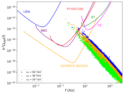
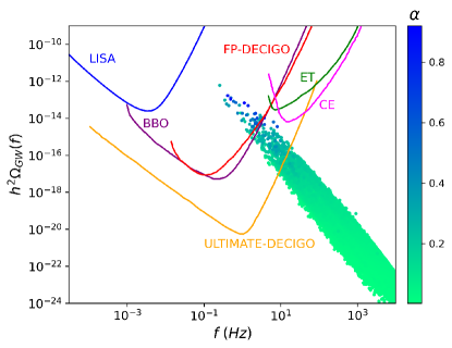
Figure 4: The peak of the GW spectrum $\Omega_{\rm{GW}}$ for points with SFOPT, along with the sensitivity curves of various upcoming GW detectors. Left panel: points corresponding to $v_{R}=20,~{}30$, and 50 TeV are shown. Right panel: Points are color-coded according to the value of $\alpha$, for $v_{R}=20,~{}30$, and 50 TeV combined.

From the expressions of $\Omega_{\rm{sw}}$ and $\Omega_{\rm{turb}}$, it is clear that large $\alpha$ and small $\beta/H_{*}$ lead to a strong GW spectrum. The peak frequency is proportional to $T_{n}\sim v_{R}$ and hence, the peak shifts to the right for larger $v_{R}$. This is illustrated in fig. 4, where we show scatter plots of the parameter points for which $\alpha,~{}\beta/H_{*}$, and $T_{n}$ have been computed. Each point represents the peak value corresponding to the GW spectrum, $h^{2}\Omega_{\text{GW}}$. The left panel shows that these points shift to the right as $v_{R}$ is progressively increased between $v_{R}=20,~{}30$ and $50$ TeV. The strength of the GW signature is not affected by varying $v_{R}$. The right panel shows the variation of $\alpha$ for the points corresponding to $v_{R}=20,~{}30$, and $50$ TeV combined. There is clearly a positive correlation between large $\alpha$ and the strength of GW. The solid lines represent the power-law integrated sensitivity curves corresponding to planned detectors such as LISA, FP-DECIGO, BBO, Ultimate-DECIGO, ET, and CE. Points lying above the sensitivity curve of a detector would have strong detection prospects. The DLRSM phase transition has good detection prospects for the detectors FP-DECIGO, BBO, and Ultimate-DECIGO for the chosen set of $v_{R}$ values. The GW spectrum is too weak to be detected at ET and CE for the chosen range of $v_{R}$. If the scale $v_{R}$ is increased by a factor of $\sim 10-100$, these two detectors may be able to detect them, but we ignore this region as the complementary collider constraints would be too weak.

Figure 5: Points with detectable GW signature at upcoming observatories: Ultimate-DECIGO, BBO, and FP-DECIGO. The scale is chosen to be, $v_{R}=20$ TeV (left panel), $v_{R}=30$ TeV (middle panel), and $v_{R}=50$ TeV (right panel). The purple, blue, and yellow contours represent the upper limits on $y_{33}=1,1.5,\sqrt{4\pi}$ respectively based on eq. (II.2).

In fig. 5 we illustrate the distribution of the points with detectable GW signal in the $r-w$ plane. The grey points pass all the theoretical and experimental constraints. The blue points are only detectable at Ultimate-DECIGO, the green points are detectable by Ultimate-DECIGO as well as BBO, and the red points can be detected at all three detectors. Interestingly, for $v_{R}=20$ TeV, the red, green, and blue points are densely clustered around $w\sim\mathcal{O}(1)$. For most of these points, $y_{33}$ is also large, $y_{33}\sim 1.5-\sqrt{4\pi}$. In the middle panel, i.e. $v_{R}=30$ TeV, the majority of points still prefer $w\sim\mathcal{O}(1)$, but now there are also points at lower values of $w$. In the case of $v_{R}=50$ TeV, we see that the clustering of points around $\mathcal{O}(1)$ values of $w$ is even more diffuse. In all three cases, i.e. $v_{R}=20,~{}30,$ and 50 TeV, there is no particular preference in the $r$ direction, as also seen from the SFOPT plots given in fig. 2.

	BP1	BP2	BP3	BP4	BP5	BP6
$v_{R}$ (TeV)	30	30	30	30	20	50
$\lambda_{0}$	0.126796	0.466090	0.308396	0.324564	1.982649	0.799371
$\lambda_{2}$	0.097015	0.253725	0.141320	0.267655	1.670007	0.413236
$\alpha_{0}$	0.004789	0.003504	0.007640	0.012450	0.012042	0.021020
$\alpha_{3}$	0.957421	0.005786	0.006466	0.004839	0.001015	0.003094
$\rho_{1}$	0.019071	0.001274	0.001929	0.005930	0.009976	0.003445
$\rho_{2}$	2.003479	0.627225	1.166146	1.674371	5.574184	2.275937
$r$	0.008261	0.008136	0.418869	0.020970	0.390416	0.424048
$w$	$4\times 10^{-6}$	0.950364	1.439902	0.766492	2.702912	2.018973
$m_{W_{R}^{\pm}}$ (TeV)	9.81	9.81	9.81	9.81	6.54	16.35
$m_{Z_{R}}$ (TeV)	11.58	11.58	11.58	11.58	7.72	19.30
$m_{H_{1}}$ (TeV)	20.72	15.97	32.79	20.89	81.06	99.90
$m_{H_{2}}$ (TeV)	29.74	23.13	45.58	34.46	116.99	144.97
$m_{H_{3}}$ (TeV)	5.86	1.51	1.86	3.27	2.82	4.15
$\alpha$	0.280	0.274	0.243	0.122	0.428	0.273
$\beta/H_{*}$	422	1050	2648	8267	975	3204
$T_{c}$ (TeV)	5.78	3.26	3.46	4.83	2.82	5.87
$T_{n}$ (TeV)	3.08	1.68	1.86	2.91	1.37	3.26

Table 1: Benchmark points for DLRSM in the simple basis.

VI Detection prospects

The prospect of detecting a GW signal in a given GW observatory can be quantified using the signal-to-noise ratio (SNR), defined as Athron:2023xlk

$${\rm{SNR}}=\sqrt{\tau\int_{f_{\rm{min}}}^{f_{\rm{max}}}df\left[\frac{\Omega_{\rm{GW}}(f)h^{2}}{\Omega_{\rm{sens}}(f)h^{2}}\right]^{2}},$$ (60)

where $\tau$ is the time period (in seconds) over which the detector is active and the integration is carried out over the entire frequency range $[f_{\rm{min}},f_{\rm{max}}]$ of the detector. For calculations, we take $\tau=2$ years. $\Omega_{\rm{sens}}(f)$ is the noise energy density power spectrum for the chosen detector. A signal is detectable if the observed SNR value exceeds a threshold SNR, denoted as $\rm{SNR_{thres}}$. We take $\rm{SNR_{thres}}=10$ for the purpose of discussion.

Table 1 presents six benchmark points (BP) with high SNR values for FP-DECIGO, BBO, and Ultimate-DECIGO, obtained using eq. (60). BP1, BP2, BP3, and BP4 have been chosen at the $SU(2)_{R}$ breaking scale $v_{R}=30$ TeV, while for BP5 and BP6 the chosen scales are $v_{R}=20$ TeV and $50$ TeV respectively. The top segment of the table shows the values of the quartic couplings, while the middle segment gives the mass spectrum corresponding to each BP. The bottom segment gives the values of PT parameters $\alpha$, $\beta/H_{*}$, $T_{c}$ and $T_{n}$. Barring BP1, all other BPs have $w\sim\mathcal{O}(1)$. All BPs have $\rho_{1}\lesssim\mathcal{O}(10^{-1})$ and hence smaller values of $m_{H_{3}}$ are preferred.

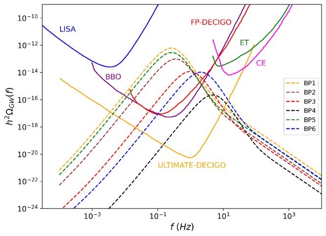
Figure 6: GW spectra for the benchmark points listed in table 1.

The full GW spectra for the BPs are shown in fig. 6. The peak of the spectrum corresponds to the frequency $f_{sw}$ defined in eq. (58) since $\Omega_{\rm{sw}}$ gives the dominant contribution. The peak of BP4 lies only above Ultimate-DECIGO and below BBO and FP-DECIGO, while all other BPs have GW peaks above the sensitivity curves of Ultimate-DECIGO, BBO, and FP-DECIGO. The low- and high-frequency tails are dominated by the power law behavior of $\Omega_{\rm{turb}}$.

The SNR of the BPs are listed in table 2. As proclaimed in the previous section, the BPs generally yield high SNR values ($\sim 10^{5}$ or above) for FP-DECIGO, BBO, and Ultimate-DECIGO. The SNR values for BP1, BP2, BP3, BP5 and BP6 are higher than $10^{5}$ for FP-DECIGO, BBO, and Ultimate-DECIGO, and hence have very good detection prospects. Ultimate-DECIGO, being the most sensitive, can detect all the BPs listed in table 2. The point BP4 is not detectable at FP-DECIGO and BBO, but can be detected by Ultimate-DECIGO.

SNR	BP1	BP2	BP3	BP4	BP5	BP6
FP-DECIGO	$1.4\times 10^{8}$	$1.8\times 10^{7}$	$5.5\times 10^{5}$	$-$	$6.8\times 10^{7}$	$1.3\times 10^{5}$
BBO	$4.0\times 10^{8}$	$6.3\times 10^{7}$	$2.8\times 10^{6}$	$-$	$1.9\times 10^{8}$	$5.9\times 10^{5}$
Ultimate-DECIGO	$1.7\times 10^{11}$	$4.4\times 10^{10}$	$1.3\times 10^{10}$	$3.6\times 10^{7}$	$8.7\times 10^{10}$	$7.7\times 10^{9}$

Table 2: SNR values corresponding to different detectors for the benchmark points.

VII Complementary collider probes

Now we describe the collider probes that complement the GW signatures discussed in the previous sections. We discuss two important collider implications, namely the precision of $\kappa_{h}$ and detection of $H_{3}$.

$\delta\kappa_{h}$	$20$ TeV	$30$ TeV	$50$ TeV	Combined
$>5\%$	$52\%$	$58\%$	$50\%$	$54\%$
$>10\%$	$21\%$	$34\%$	$33\%$	$30\%$
$>20\%$	$8\%$	$20\%$	$25\%$	$17\%$
$>50\%$	$1.3\%$	$12\%$	$15\%$	$9\%$

Table 3: Percentage of points detectable at Ultimate-DECIGO to be ruled out when the sensitivity of $\kappa_{h}$ reaches $5\%,10\%,20\%,$ and $50\%$, for $v_{R}=20,30,$ and $50\,$TeV.

• As argued in Sec. II.5, in DLRSM the trilinear Higgs coupling can deviate significantly from its SM value. In Table 3, we present the percentage of points leading to detectable GW signal at Ultimate-DECIGO, which also show deviation of $\kappa_{h}$ at $5\%,~{}10\%,~{}20\%,$ and $50\%$. The current ATLAS measurement allows for a rather large range of $\kappa_{h}\in[-2.3,10.3]$. However, future colliders will significantly tighten the bound. Here we quote the projected sensitivities of $\kappa_{h}$ from ref. deBlas:2019rxi . HL-LHC will achieve a sensitivity of $50\%$ from the di-Higgs production channel. The proposed colliders, such as HE-LHC, CLIC₃₀₀₀, and FCC-hh are expected improve the sensitivity of $\kappa_{h}$ to $\sim 20\%,10\%,$ and $5\%$ respectively. These colliders therefore will rule out a considerable number of points showing a strong GW signal.

  

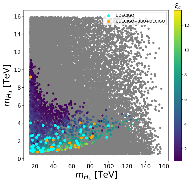
  Figure 7: The mass spectrum of DLRSM for $v_{R}=20$ TeV depicting points with $\xi_{c}>1$. The cyan and orange points lead to a GW signal detectable at Ultimate-DECIGO and Ultimate-DECIGO+BBO+FP-DECIGO respectively.

• The scalar $H_{3}$ can be produced at $pp$ colliders through several channels, for example Dev:2016dja ,

  1. $H_{1}$-decay, $pp\rightarrow H_{1}\rightarrow hH_{3}$,

  2. decay of boosted $h$, $pp\rightarrow h^{*}\rightarrow hH_{3},H_{3}H_{3}$,

  3. Higgsstrahlung, $pp\rightarrow V_{R}^{*}\rightarrow V_{R}H_{3}$,

  4. $V_{R}V_{R}$ fusion, $pp\rightarrow H_{3}jj$  .

  The relative strength of these processes depends on the mass spectrum of DLRSM.In fig. 7, we show the distribution of SFOPT points in the $m_{H_{1}}-m_{H_{3}}$ plane for $v_{R}=20$ TeV, overlaid with points which are detectable at Ultimate-DECIGO, BBO, and FP-DECIGO. The detectable points mostly occur for small $m_{H_{3}}$, with the minimum value of $m_{H_{3}}=741$ GeV. For the range $m_{H_{3}}=740$ GeV $-$ 1.2 TeV, the production cross-section of $H_{3}$ at FCC-hh with $\sqrt{s}=100$ TeV can be $\sim\mathcal{O}(\text{fb})$ Dev:2016dja .

  For $v_{R}=20$ TeV, $m_{H_{3}}\lesssim 500$ GeV can be ruled out from the observations of the channel (iv) at FCC-hh with a luminosity of $30\,\text{ab}^{-1}$. For large values of quartic couplings, the decay width $h^{*}\rightarrow hH_{3}$ and $h^{*}\rightarrow H_{3}H_{3}$ can be large and subsequently, channel (ii) can rule out $m_{H_{3}}\lesssim 700$ GeV. For channel (i), $H_{1}$ with mass $15$ TeV can be produced with a cross-section $\sim 0.5$ fb and have sizable branching ratios of $H_{1}\rightarrow hH_{3},\,H_{3}H_{3}$. As a result, channel (i) can rule out masses up to $m_{H_{3}}\sim 2$ TeV. Thus, these searches are capable of ruling out a large number of points with low-$m_{H_{3}}$, thus low-$\rho_{1}$, providing a complementarity to the GW probe of DLRSM.

VIII Summary and conclusions

In this paper, we studied the possibility of an observable stochastic GW background resulting from SFOPT associated with the spontaneous breaking of $SU(2)_{R}\times U(1)_{B-L}$ in DLRSM. The gauge symmetry of DLRSM breaks in the following pattern:

$$SU(2)_{L}\times SU(2)_{R}\times U(1)_{B-L}\xrightarrow{\mathit{~{}~{}v_{R}~{}~{}}}SU(2)_{L}\times U(1)_{Y}\xrightarrow{\mathit{\kappa_{1},\kappa_{2},v_{L}}}U(1)_{Y}.$$

The non-observation of a right-handed current at colliders puts a lower bound on the scale $v_{R}$ to be around 20 TeV. Due to the hierarchy $v_{R}\gg v$, the $SU(2)_{R}\times U(1)_{B-L}$-breaking dynamics is decoupled from the EWPT. We chose the scale $v_{R}=20,~{}30,$ and $50$ TeV to study the possible detection of GW background at the planned observatories. For these values of $v_{R}$, complementary searches for new scalars of DLRSM are feasible at future colliders.

We imposed a discrete left-right symmetry on the model. Our analysis was carried out using the simple basis defined in ref. Karmakar:2022iip , to reduce the number of independent parameters. It should be noted that analysis with the full set of parameters also gives similar patterns of SFOPT in the $\rho_{1}-\rho_{2}$ and $r-w$ planes. The parameters in the simple basis include the quartic couplings: $\lambda_{0},\lambda_{2},\alpha_{0},\alpha_{3},\rho_{1},\rho_{2}$. In addition, we defined EW vevs through the ratios $r$ and $w$. Most studies on LRSM take the simplified limit $r,w\rightarrow 0$. However, it was pointed out in refs. Bernard:2020cyi ; Karmakar:2022iip that the DLRSM phenomenology allows for significant deviation from this limit. Therefore, we also scanned over $r$ and $w$.

We constructed the one-loop finite temperature effective potential for each parameter point and analyzed the nature of PT using the package CosmoTransitions. Due to the large separation between $v_{R}$ and the EW scale, the effective potential depends solely on the background field value of the neutral CP-even scalar, $\chi^{0}_{Rr}$. The condition for SFOPT, $\xi_{c}>1$ was used to identify viable regions of the parameter space. SFOPT favors small values of the quartic coupling $\rho_{1}\lesssim\mathcal{O}(10^{-1})$, which leads to $m_{H_{3}}\ll v_{R}$. This feature has also been observed in other variants of LRSM, discussed in refs. Brdar:2019fur ; Graf:2021xku ; Li:2020eun .

For very small values, $\rho_{1}\lesssim 10^{-3}$ however, the zero temperature minimum of the one-loop effective potential at $R=v_{R}$ becomes metastable, violating the Linde-Weinberg bound. Hence there is a lower bound on $\rho_{1}$ below which FOPT is not observed. Most points with SFOPT also feature $w\sim\mathcal{O}(1)$, while for smaller values of $w$, very few points show SFOPT. Out of the chosen set of parameters, the SFOPT region is most sensitive to the parameters $\rho_{1}$ and $w$ and to some extent $\lambda_{0}$. However, we see no particular preference for the vev ratio $r$ and the quartic couplings relating the bidoublet and the doublet fields, i.e., $\alpha_{0}$ and $\alpha_{3}$, as illustrated by the projections given in fig. 2.

For parameter points showing SFOPT, we computed the PT parameters, $\alpha$, $\beta/H_{*}$, and $T_{n}$, needed for the calculation of the GW spectrum. In the non-runaway scenario, the stochastic GW background resulting from SFOPT comes primarily from sound waves and turbulence, while the contribution from bubble wall collisions remains sub-dominant. Fig. 4 shows the position of the peak of the GW spectrum for points satisfying the SFOPT criterion. While for a large number of points, the GW spectrum is too weak to be detected, there is a significant number of points lying above the sensitivity curves for Ultimate-DECIGO, BBO, and FP-DECIGO. Such points will be accessible to these detectors in the coming years. The detectable points also prefer $w\sim\mathcal{O}(1)$, which in turn, correspond to a large value of $y_{33}$ as seen in fig. 5.

The strength of the GW spectrum does not depend on the scale $v_{R}$. On the other hand, since the peak frequency is proportional to $T_{n}\sim v_{R}$, the points shift to the right as $v_{R}$ changes from $20$ to $30$ to $50$ TeV. To quantify the detection prospects, we computed the signal-to-noise ratio at these detectors for the detectable points. Six benchmark points are given in table 2, featuring SNR values higher than $10^{5}$. We see that for all the BPs, $m_{H_{3}}\lesssim 5$ TeV.

There are primarily two complementary collider probes for the points with detectable GW signals. It was found that a significant fraction of points leads to $50,20,10,\text{and}\,5\%$ deviation of $k_{h}$ from unity, which can be ruled out at HL-LHC, HE-LHC, CLIC₃₀₀₀, and FCC-hh respectively. Due to a relatively low mass of $H_{3}$, it can be produced at future colliders through various channels. In particular, FCC-hh can rule out up to $m_{H_{3}}\sim 2$ TeV.

Although DLRSM does not account for neutrino masses, it is interesting to ask if incorporating them by adding extra fields to the model could modify the strength of FOPT. In Appendix C, we show that it is possible to include neutrino masses without impacting the results of our analysis.

Here we also note that the discrete LR symmetry imposed on the model also breaks spontaneously during the $SU(2)_{R}\times U(1)_{B-L}\rightarrow U(1)_{Y}$ PT, leading to the formation of domain walls. The domain wall problem can be avoided by introducing explicit LR-breaking terms in the potential. These domain walls can also produce a stochastic GW background peaking at very low frequencies, possibly detectable by pulsar timing arrays.

Appendix A Minimization at the EW vacua

The minimization conditions are given by:

$$\mu_{1}^{2} = \frac{1}{2(r^{2}-1)}\Bigg{(}\kappa_{1}^{2}\Big{(}w^{2}((r^{2}-1)\alpha_{1}+r^{2}\alpha_{3}-\alpha_{4})+2(r^{2}-1)((r^{2}+1)\lambda_{1}+2r\lambda_{4})\Big{)}$$

$$+2\sqrt{2}rv_{R}w\mu_{4}+v_{R}^{2}\Big{(}(r^{2}-1)\alpha_{1}+r^{2}\alpha_{3}-\alpha_{4}+2w^{2}\rho_{12}\Big{)}\Bigg{)}\,\,,$$

$$\mu_{2}^{2} = \frac{1}{4(r^{2}-1)}\Bigg{(}\kappa_{1}^{2}\Big{(}w^{2}(r^{2}-1)\alpha_{2}-w^{2}r\alpha_{34}+2(r^{2}-1)(2r\lambda_{23}+(r^{2}+1)\lambda_{4})\Big{)}$$

$$-\sqrt{2}(r^{2}+1)v_{R}w\mu_{4}+v_{R}^{2}\Big{(}(r^{2}-1)\alpha_{2}-r\alpha_{34}-2w^{2}\rho_{12}\Big{)}\Bigg{)}\,\,,$$

$$\mu_{3}^{2} = \frac{1}{2}\kappa_{1}^{2}((r^{2}+1)\alpha_{1}+2r\alpha_{2}+r^{2}\alpha_{3}+\alpha_{4}+2w^{2}\rho_{1})+v_{R}^{2}\rho_{1}\,\,,$$

$$\mu_{5} = -r\mu_{4}-\sqrt{2}v_{R}w\rho_{12},$$ (61)

where, $\rho_{12}=\rho_{2}/2-\rho_{1}$, $\alpha_{34}=\alpha_{3}-\alpha_{4}$, and $\lambda_{23}=2\lambda_{2}+\lambda_{3}$.

Appendix B Field-dependent masses

The field-dependent mass matrices are obtained from the tree-level effective potential:

$$m^{2}_{ij}(R)=\left.\frac{\partial^{2}}{\partial\varphi_{i}\partial\varphi_{j}}V_{0}\right|_{\langle\cdots\rangle}$$ (62)

where $\langle\cdots\rangle$ denotes the background field value.

For the CP-even sector, we obtain,

$$\mathcal{M}^{2}_{\rm{CPE}}=\begin{pmatrix}-\mu_{1}^{2}+\frac{1}{2}(\alpha_{1}+\alpha_{4})R^{2}&-2\mu_{2}^{2}+\frac{1}{2}\alpha_{2}R^{2}&\frac{1}{\sqrt{2}}\mu_{5}R&0\\ -2\mu_{2}^{2}+\frac{1}{2}\alpha_{2}R^{2}&-\mu_{1}^{2}+\frac{1}{2}(\alpha_{1}+\alpha_{3})R^{2}&\frac{1}{\sqrt{2}}\mu_{4}R&0\\ \frac{1}{\sqrt{2}}\mu_{5}R&\frac{1}{\sqrt{2}}\mu_{4}R&-\mu_{3}^{2}+\frac{1}{2}\rho_{2}R^{2}&0\\ 0&0&0&-\mu_{3}^{2}+3\rho_{1}R^{2}\\ \end{pmatrix}.$$ (63)

For the CP-odd scalars,

$$\mathcal{M}^{2}_{\rm{CP0}}=\begin{pmatrix}-\mu_{1}^{2}+\frac{1}{2}(\alpha_{1}+\alpha_{4})R^{2}&2\mu_{2}^{2}-\frac{1}{2}\alpha_{2}R^{2}&-\frac{1}{\sqrt{2}}\mu_{5}R&0\\ 2\mu_{2}^{2}-\frac{1}{2}\alpha_{2}R^{2}&-\mu_{1}^{2}+\frac{1}{2}(\alpha_{1}+\alpha_{3})R^{2}&\frac{1}{\sqrt{2}}\mu_{4}R&0\\ -\frac{1}{\sqrt{2}}\mu_{5}R&\frac{1}{\sqrt{2}}\mu_{4}R&-\mu_{3}^{2}+\frac{1}{2}\rho_{2}R^{2}&0\\ 0&0&0&-\mu_{3}^{2}+\rho_{1}R^{2}\\ \end{pmatrix},$$ (64)

and for the charged scalars, we get,

$$\mathcal{M}^{2}_{\rm{charged}}=\begin{pmatrix}-\mu_{1}^{2}+\frac{1}{2}(\alpha_{1}+\alpha_{4})R^{2}&2\mu_{2}^{2}-\frac{1}{2}\alpha_{2}R^{2}&-\frac{1}{\sqrt{2}}\mu_{5}R&0\\ 2\mu_{2}^{2}-\frac{1}{2}\alpha_{2}R^{2}&-\mu_{1}^{2}+\frac{1}{2}(\alpha_{1}+\alpha_{3})R^{2}&\frac{1}{\sqrt{2}}\mu_{4}R&0\\ -\frac{1}{\sqrt{2}}\mu_{5}R&\frac{1}{\sqrt{2}}\mu_{4}R&-\mu_{3}^{2}+\frac{1}{2}\rho_{2}R^{2}&0\\ 0&0&0&-\mu_{3}^{2}+\rho_{1}R^{2}\\ \end{pmatrix}.$$ (65)

For the neutral gauge bosons, we have the mass matrix,

$$\mathcal{M}^{2}_{Z}=\begin{pmatrix}0&0&0\\ 0&0&0\\ 0&\frac{1}{4}g_{R}^{2}R^{2}&-\frac{1}{4}g_{BL}g_{R}R^{2}\\ 0&-\frac{1}{4}g_{BL}g_{R}R^{2}&\frac{1}{4}g_{BL}^{2}R^{2}\\ \end{pmatrix}.$$ (66)

For the charged bosons,

$$\mathcal{M}^{2}_{W}=\begin{pmatrix}0&0\\ 0&\frac{1}{4}g_{R}^{2}R^{2}\\ \end{pmatrix}.$$ (67)

In addition to the field-dependent masses, we also need thermal self-energies of the fields for daisy resummation. These are obtained from the high-T expansion of the one-loop thermal potential. Substituting eq. (32) in eq. (30) gives, to leading order,

$$V_{1T}^{\rm{high}}=\frac{T^{2}}{24}\left(\sum_{b}n_{b}m_{b}^{2}+\frac{1}{2}\sum_{f}n_{f}m_{f}^{2}\right).$$ (68)

Here, index $b$ runs over bosons, while index $f$ runs over fermions. Each sum can be expressed as the trace of the respective matrix. Thermal mass matrices are then expressed as, $\Pi_{ij}=c_{ij}T^{2}$, where $c_{ij}$ are,

$$c_{ij}=\frac{1}{T^{2}}\left.\frac{\partial^{2}}{\partial\varphi_{i}\partial\varphi_{j}}V_{1T}^{\rm{high}}\right|_{\langle\cdots\rangle}.$$ (69)

We define,

$$d_{1} = \frac{1}{48}(9g_{L}^{2}+9g_{R}^{2}+8(2\alpha_{1}+\alpha_{3}+\alpha_{4}+5\lambda_{1}+2\lambda_{3})),$$ (70)

$$d^{\prime}_{1} = d_{1}+\frac{y_{33}^{2}}{4}+\frac{\tilde{y}_{33}^{2}}{4},$$ (71)

$$d_{2} = \frac{1}{3}(2\alpha_{2}+3\lambda_{4}),$$ (72)

$$d^{\prime}_{2} = d_{2}+\frac{y_{33}\tilde{y}_{33}}{4},$$ (73)

$$d_{L} = \frac{1}{48}(3g_{BL}^{2}+9g_{L}^{2}+8(2\alpha_{1}+\alpha_{3}+\alpha_{4}+3\rho_{1}+\rho_{2})),$$ (74)

$$d_{R} = \frac{1}{48}(3g_{BL}^{2}+9g_{R}^{2}+8(2\alpha_{1}+\alpha_{3}+\alpha_{4}+3\rho_{1}+\rho_{2}))\,.$$ (75)

We obtain the following thermal mass matrices:

$$\Pi_{\rm{CPE}}=T^{2}\begin{pmatrix}d^{\prime}_{1}&d^{\prime}_{2}&0&0\\ d^{\prime}_{2}&d^{\prime}_{1}&0&0\\ 0&0&d_{L}&0\\ 0&0&0&d_{R}\\ \end{pmatrix},$$ (76)

$$\Pi_{\rm{CP0}}=T^{2}\begin{pmatrix}d^{\prime}_{1}&-d^{\prime}_{2}&0&0\\ -d^{\prime}_{2}&d^{\prime}_{1}&0&0\\ 0&0&d_{L}&0\\ 0&0&0&d_{R}\\ \end{pmatrix},$$ (77)

$$\Pi_{\rm{charged}}=T^{2}\begin{pmatrix}d_{1}&-d_{2}&0&0\\ -d_{2}&d_{1}&0&0\\ 0&0&d_{L}&0\\ 0&0&0&d_{R}\\ \end{pmatrix}.$$ (78)

The gauge boson thermal mass matrices are,

$$\Pi_{Z}=\frac{T^{2}}{6}\begin{pmatrix}13g_{L}^{2}&0&0\\ 0&13g_{R}^{2}&0\\ 0&0&6g_{BL}^{2}\\ \end{pmatrix},$$ (79)

$$\Pi_{W}=\frac{13}{6}T^{2}\begin{pmatrix}g_{L}^{2}&0\\ 0&g_{R}^{2}\\ \end{pmatrix}.$$ (80)

Appendix C Neutrino masses in DLRSM

We have not taken into account a mechanism for generating neutrino mass in our version of DLRSM. In this section, we argue the minimal way of incorporating neutrino mass in this model do not give any additional contribution to the GW phenomenology of the model.

To demonstrate our point, we consider the model discussed in refs. FileviezPerez:2016erl ; FileviezPerez:2017zwm . Small neutrino masses are generated radiatively by the Zee mechanism, by adding a charged singlet scalar $\delta^{+}\sim(1,1,1,2)$ to DLRSM. In our notation, the Majorana Lagrangian is,

$$-\mathcal{L}^{M}_{LR}=\gamma_{L}L_{L}L_{L}\delta^{+}+\gamma_{R}L_{R}L_{R}\delta^{+}+\gamma_{1}\chi_{L}^{T}i\sigma_{2}\Phi\chi_{R}\delta^{-}+\gamma_{1}\chi_{L}^{T}i\sigma_{2}\tilde{\Phi}\chi_{R}\delta^{-}+\text{h.c.}\,,$$ (81)

where, $\gamma_{L,R},~{}\gamma_{1},~{}\gamma_{2}$ are the new Yukawa couplings. As there is no tree-level right-handed neutrino mass, the contribution of the RH neutrinos to the effective potential is zero. However, the quartic terms involving $\delta^{+}$ modify the mixing between the charged scalars. In the basis of $\{\phi_{1}^{\pm},\phi_{2}^{\pm},\chi_{L}^{\pm},\chi_{R}^{\pm},\delta^{\pm}\}$, the additional contribution to the charged mass matrix, $\mathcal{M}^{2}_{\rm{}_{charged}}$ is,

$$\delta\mathcal{M}^{2}_{\rm{}_{charged}}=v_{R}^{2}\begin{pmatrix}0&0&0&0&\frac{\gamma_{2}}{2}\frac{v_{L}}{v_{R}}\\ 0&0&0&0&-\frac{\gamma_{1}}{2}\frac{v_{L}}{v_{R}}\\ 0&0&0&0&\frac{(\gamma_{1}\kappa_{2}+\gamma_{2}\kappa_{1})}{2v_{R}}\\ 0&0&0&0&-\frac{v_{L}(\gamma_{1}\kappa_{1}+\gamma_{2}\kappa_{2})}{2v_{R}^{2}}\\ \frac{\gamma_{2}}{2}\frac{v_{L}}{v_{R}}&-\frac{\gamma_{1}}{2}\frac{v_{L}}{v_{R}}&\frac{(\gamma_{1}\kappa_{2}+\gamma_{2}\kappa_{1})}{2v_{R}}&-\frac{v_{L}(\gamma_{1}\kappa_{1}+\gamma_{2}\kappa_{2})}{2v_{R}^{2}}&0\end{pmatrix}.$$ (82)

Each of the non-zero entries is suppressed by a factor $v_{L}/v_{R}$ or $\kappa_{1,2}/v_{R}$ compared to $v_{R}^{2}$. Therefore the mixing of the charged scalars of DLRSM with $\delta^{+}$ is negligible, while their mixing among themselves remains unchanged. In the field-dependent mass matrix, we put $v_{L}\rightarrow 0,~{}\kappa_{1,2}\rightarrow 0$, and $v_{R}\rightarrow R$, by which the additional mixing matrix, $\delta\mathcal{M}^{2}_{\rm{}_{charged}}(R)$, vanishes entirely. Hence the presence of $\delta^{+}$ does not alter the field-dependent mass matrices and therefore does not contribute to the effective potential.

References

- (1) J. C. Pati and A. Salam, “Lepton Number as the Fourth Color,” Phys. Rev. D 10 (1974) 275–289. [Erratum: Phys.Rev.D 11, 703–703 (1975)].
- (2) R. N. Mohapatra and J. C. Pati, “A Natural Left-Right Symmetry,” Phys. Rev. D 11 (1975) 2558.
- (3) R. N. Mohapatra and J. C. Pati, “Left-right gauge symmetry and an ”isoconjugate” model of violation,” Phys. Rev. D 11 (Feb, 1975) 566–571. https://link.aps.org/doi/10.1103/PhysRevD.11.566.
- (4) G. Senjanovic and R. N. Mohapatra, “Exact Left-Right Symmetry and Spontaneous Violation of Parity,” Phys. Rev. D 12 (1975) 1502.
- (5) G. Senjanovic, “Spontaneous Breakdown of Parity in a Class of Gauge Theories,” Nucl. Phys. B 153 (1979) 334–364.
- (6) A. Maiezza, G. Senjanović, and J. C. Vasquez, “Higgs sector of the minimal left-right symmetric theory,” Phys. Rev. D 95 no. 9, (2017) 095004, arXiv:1612.09146 [hep-ph].
- (7) N. G. Deshpande, J. F. Gunion, B. Kayser, and F. Olness, “Left-right-symmetric electroweak models with triplet higgs field,” Phys. Rev. D 44 (Aug, 1991) 837–858. https://link.aps.org/doi/10.1103/PhysRevD.44.837.
- (8) G. Senjanovic, “Is left–right symmetry the key?,” Mod. Phys. Lett. A 32 no. 04, (2017) 1730004, arXiv:1610.04209 [hep-ph].
- (9) R. N. Mohapatra and D. P. Sidhu, “Gauge Theories of Weak Interactions with Left-Right Symmetry and the Structure of Neutral Currents,” Phys. Rev. D 16 (1977) 2843.
- (10) K. S. Babu and V. S. Mathur, “Radiatively Induced Seesaw Mechanism for Neutrino Masses,” Phys. Rev. D 38 (1988) 3550.
- (11) P. Fileviez Perez, C. Murgui, and S. Ohmer, “Simple Left-Right Theory: Lepton Number Violation at the LHC,” Phys. Rev. D 94 no. 5, (2016) 051701, arXiv:1607.00246 [hep-ph].
- (12) P. Fileviez Perez and C. Murgui, “Lepton Flavour Violation in Left-Right Theory,” Phys. Rev. D 95 no. 7, (2017) 075010, arXiv:1701.06801 [hep-ph].
- (13) K. S. Babu and A. Thapa, “Left-Right Symmetric Model without Higgs Triplets,” arXiv:2012.13420 [hep-ph].
- (14) E. Ma, “Dark-Matter Fermion from Left-Right Symmetry,” Phys. Rev. D 85 (2012) 091701, arXiv:1202.5828 [hep-ph].
- (15) M. Frank, C. Majumdar, P. Poulose, S. Senapati, and U. A. Yajnik, “Exploring and leptogenesis in the alternative left-right model,” Phys. Rev. D 102 no. 7, (2020) 075020, arXiv:2008.12270 [hep-ph].
- (16) L. Gráf, S. Jana, A. Kaladharan, and S. Saad, “Gravitational wave imprints of left-right symmetric model with minimal Higgs sector,” JCAP 05 no. 05, (2022) 003, arXiv:2112.12041 [hep-ph].
- (17) B. A. et al., “Observation of gravitational waves from a binary black hole merger,” Physical Review Letters 116 no. 6, (Feb, 2016) . https://doi.org/10.1103%2Fphysrevlett.116.061102.
- (18) LIGO Scientific Collaboration, G. M. Harry, “Advanced LIGO: The next generation of gravitational wave detectors,” Class. Quant. Grav. 27 (2010) 084006.
- (19) VIRGO Collaboration, T. Accadia et al., “Virgo: a laser interferometer to detect gravitational waves,” JINST 7 (2012) P03012.
- (20) LISA Collaboration, P. Amaro-Seoane et al., “Laser Interferometer Space Antenna,” arXiv:1702.00786 [astro-ph.IM].
- (21) N. Seto, S. Kawamura, and T. Nakamura, “Possibility of direct measurement of the acceleration of the universe using 0.1-Hz band laser interferometer gravitational wave antenna in space,” Phys. Rev. Lett. 87 (2001) 221103, arXiv:astro-ph/0108011.
- (22) V. Corbin and N. J. Cornish, “Detecting the cosmic gravitational wave background with the big bang observer,” Class. Quant. Grav. 23 (2006) 2435–2446, arXiv:gr-qc/0512039.
- (23) M. Punturo et al., “The Einstein Telescope: A third-generation gravitational wave observatory,” Class. Quant. Grav. 27 (2010) 194002.
- (24) LIGO Scientific Collaboration, B. P. Abbott et al., “Exploring the Sensitivity of Next Generation Gravitational Wave Detectors,” Class. Quant. Grav. 34 no. 4, (2017) 044001, arXiv:1607.08697 [astro-ph.IM].
- (25) C. Caprini et al., “Science with the space-based interferometer eLISA. II: Gravitational waves from cosmological phase transitions,” JCAP 04 (2016) 001, arXiv:1512.06239 [astro-ph.CO].
- (26) P. Athron, C. Balázs, A. Fowlie, L. Morris, and L. Wu, “Cosmological phase transitions: from perturbative particle physics to gravitational waves,” arXiv:2305.02357 [hep-ph].
- (27) LISA Cosmology Working Group Collaboration, P. Auclair et al., “Cosmology with the Laser Interferometer Space Antenna,” Living Rev. Rel. 26 no. 1, (2023) 5, arXiv:2204.05434 [astro-ph.CO].
- (28) C. Caprini and D. G. Figueroa, “Cosmological Backgrounds of Gravitational Waves,” Class. Quant. Grav. 35 no. 16, (2018) 163001, arXiv:1801.04268 [astro-ph.CO].
- (29) P. S. B. Dev and A. Mazumdar, “Probing the Scale of New Physics by Advanced LIGO/VIRGO,” Phys. Rev. D 93 no. 10, (2016) 104001, arXiv:1602.04203 [hep-ph].
- (30) A. Addazi, A. Marcianò, and R. Pasechnik, “Probing Trans-electroweak First Order Phase Transitions from Gravitational Waves,” MDPI Physics 1 no. 1, (2019) 92–102, arXiv:1811.09074 [hep-ph].
- (31) D. Ringe, “Probing intermediate scale Froggatt-Nielsen models at future gravitational wave observatories,” Phys. Rev. D 107 no. 1, (2023) 015030, arXiv:2208.07778 [hep-ph].
- (32) V. Brdar, L. Graf, A. J. Helmboldt, and X.-J. Xu, “Gravitational Waves as a Probe of Left-Right Symmetry Breaking,” JCAP 12 (2019) 027, arXiv:1909.02018 [hep-ph].
- (33) M. Li, Q.-S. Yan, Y. Zhang, and Z. Zhao, “Prospects of gravitational waves in the minimal left-right symmetric model,” JHEP 03 (2021) 267, arXiv:2012.13686 [hep-ph].
- (34) D. Borah and A. Dasgupta, “Probing left-right symmetry via gravitational waves from domain walls,” Phys. Rev. D 106 no. 3, (2022) 035016, arXiv:2205.12220 [hep-ph].
- (35) V. Bernard, S. Descotes-Genon, and L. Vale Silva, “Constraining the gauge and scalar sectors of the doublet left-right symmetric model,” JHEP 09 (2020) 088, arXiv:2001.00886 [hep-ph].
- (36) S. Karmakar, J. More, A. K. Pradhan, and S. U. Sankar, “Constraints on the doublet left-right symmetric model from Higgs data,” JHEP 03 (2023) 168, arXiv:2211.08445 [hep-ph].
- (37) Y. Zhang, H. An, X. Ji, and R. N. Mohapatra, “General CP Violation in Minimal Left-Right Symmetric Model and Constraints on the Right-Handed Scale,” Nucl. Phys. B 802 (2008) 247–279, arXiv:0712.4218 [hep-ph].
- (38) P. S. B. Dev, R. N. Mohapatra, and Y. Zhang, “Probing the Higgs Sector of the Minimal Left-Right Symmetric Model at Future Hadron Colliders,” JHEP 05 (2016) 174, arXiv:1602.05947 [hep-ph].
- (39) ATLAS Collaboration, G. Aad et al., “Search for a heavy charged boson in events with a charged lepton and missing transverse momentum from collisions at TeV with the ATLAS detector,” Phys. Rev. D 100 no. 5, (2019) 052013, arXiv:1906.05609 [hep-ex].
- (40) CMS Collaboration, S. Chatrchyan et al., “Observation of a New Boson at a Mass of 125 GeV with the CMS Experiment at the LHC,” Phys. Lett. B 716 (2012) 30–61, arXiv:1207.7235 [hep-ex].
- (41) ATLAS Collaboration, “A combination of measurements of Higgs boson production and decay using up to fb-1 of proton–proton collision data at 13 TeV collected with the ATLAS experiment,”.
- (42) ATLAS Collaboration, “Constraints on the Higgs boson self-coupling from the combination of single-Higgs and double-Higgs production analyses performed with the ATLAS experiment,”.
- (43) M. Quiros, “Finite temperature field theory and phase transitions,” in ICTP Summer School in High-Energy Physics and Cosmology, pp. 187–259. 1, 1999. arXiv:hep-ph/9901312.
- (44) M. Laine and A. Vuorinen, Basics of Thermal Field Theory, vol. 925. Springer, 2016. arXiv:1701.01554 [hep-ph].
- (45) S. R. Coleman and E. J. Weinberg, “Radiative Corrections as the Origin of Spontaneous Symmetry Breaking,” Phys. Rev. D 7 (1973) 1888–1910.
- (46) L. Dolan and R. Jackiw, “Symmetry Behavior at Finite Temperature,” Phys. Rev. D 9 (1974) 3320–3341.
- (47) J. M. Cline and P.-A. Lemieux, “Electroweak phase transition in two higgs doublet models,” Physical Review D 55 no. 6, (Mar, 1997) 3873–3881. https://doi.org/10.1103%2Fphysrevd.55.3873.
- (48) M. E. Carrington, “The Effective potential at finite temperature in the Standard Model,” Phys. Rev. D 45 (1992) 2933–2944.
- (49) R. R. Parwani, “Resummation in a hot scalar field theory,” Phys. Rev. D 45 (1992) 4695, arXiv:hep-ph/9204216. [Erratum: Phys.Rev.D 48, 5965 (1993)].
- (50) P. Arnold and O. Espinosa, “Effective potential and first-order phase transitions: Beyond leading order,” Phys. Rev. D 47 (Apr, 1993) 3546–3579. https://link.aps.org/doi/10.1103/PhysRevD.47.3546.
- (51) S. Weinberg, “Gauge and Global Symmetries at High Temperature,” Phys. Rev. D 9 (1974) 3357–3378.
- (52) C. Kilic and S. Swaminathan, “Can A Pseudo-Nambu-Goldstone Higgs Lead To Symmetry Non-Restoration?,” JHEP 01 (2016) 002, arXiv:1508.05121 [hep-ph].
- (53) P. Meade and H. Ramani, “Unrestored Electroweak Symmetry,” Phys. Rev. Lett. 122 no. 4, (2019) 041802, arXiv:1807.07578 [hep-ph].
- (54) A. D. Linde, “Dynamical Symmetry Restoration and Constraints on Masses and Coupling Constants in Gauge Theories,” JETP Lett. 23 (1976) 64–67.
- (55) S. Weinberg, “Mass of the Higgs Boson,” Phys. Rev. Lett. 36 (1976) 294–296.
- (56) C. L. Wainwright, “CosmoTransitions: Computing Cosmological Phase Transition Temperatures and Bubble Profiles with Multiple Fields,” Comput. Phys. Commun. 183 (2012) 2006–2013, arXiv:1109.4189 [hep-ph].
- (57) M. Quiros, “Field theory at finite temperature and phase transitions,” Helv. Phys. Acta 67 (1994) 451–583.
- (58) A. D. Linde, “Fate of the False Vacuum at Finite Temperature: Theory and Applications,” Phys. Lett. B 100 (1981) 37–40.
- (59) W.-C. Huang, F. Sannino, and Z.-W. Wang, “Gravitational Waves from Pati-Salam Dynamics,” Phys. Rev. D 102 no. 9, (2020) 095025, arXiv:2004.02332 [hep-ph].
- (60) J. R. Espinosa, T. Konstandin, J. M. No, and G. Servant, “Energy Budget of Cosmological First-order Phase Transitions,” JCAP 06 (2010) 028, arXiv:1004.4187 [hep-ph].
- (61) Planck Collaboration, N. Aghanim et al., “Planck 2018 results. VI. Cosmological parameters,” Astron. Astrophys. 641 (2020) A6, arXiv:1807.06209 [astro-ph.CO]. [Erratum: Astron.Astrophys. 652, C4 (2021)].
- (62) H.-K. Guo, K. Sinha, D. Vagie, and G. White, “Phase Transitions in an Expanding Universe: Stochastic Gravitational Waves in Standard and Non-Standard Histories,” JCAP 01 (2021) 001, arXiv:2007.08537 [hep-ph].
- (63) J. de Blas et al., “Higgs Boson Studies at Future Particle Colliders,” JHEP 01 (2020) 139, arXiv:1905.03764 [hep-ph].