Demystifying Visual Features of Movie Posters for Multi-Label Genre Identification

Abstract

In the film industry, movie posters have been an essential part of advertising and marketing for many decades, and continue to play a vital role even today in the form of digital posters through online, social media and OTT platforms. Typically, movie posters can effectively promote and communicate the essence of a film, such as its genre, visual style/ tone, vibe and storyline cue/ theme, which are essential to attract potential viewers. Identifying the genres of a movie often has significant practical applications in recommending the film to target audiences. Previous studies on movie genre identification are limited to subtitles, plot synopses, and movie scenes that are mostly accessible after the movie release. Posters usually contain pre-release implicit information to generate mass interest. In this paper, we work for automated multi-label genre identification only from movie poster images, without any aid of additional textual/meta-data information about movies, which is one of the earliest attempts of its kind. Here, we present a deep transformer network with a probabilistic module to identify the movie genres exclusively from the poster. For experimental analysis, we procured 13882 number of posters of 13 genres from the Internet Movie Database (IMDb), where our model performances were encouraging and even outperformed some major contemporary architectures.

I Introduction

In the contemporary landscape of the film industry, where digital platforms have revolutionized the way we consume content, the role of movie posters has undergone a profound transformation. These visual canvases, once primarily relegated to theater exhibits, newspaper ads, and DVD covers, have emerged as powerful tools for attracting audiences in the era of online streaming [1]. A movie poster is no longer just a piece of promotional artwork; it has become a gateway to a cinematic experience, a glimpse into the world of a film, and a crucial factor in a viewer’s decision-making process. Beyond their aesthetic appeal, movie posters are rich repositories of information. They convey not only the visual aesthetics of a film but also subtle cues about its genre, style, and thematic content. A well-crafted poster can encapsulate the essence of a movie, enticing viewers with tantalizing glimpses of its narrative and emotional landscape. As viewers increasingly turn to online platforms to discover and enjoy films, movie posters have assumed a pivotal role in the digital realm, guiding users in their quest for cinematic satisfaction [2].

In this digital age, where the sheer volume of available content can be overwhelming, accurate genre categorization has become paramount. Audiences rely on genre labels to navigate the expansive catalogs of online streaming platforms, seeking films that resonate with their tastes and preferences [3]. This reliance on genre categorization underscores the critical role that automated genre identification plays in enhancing the discoverability of films and improving the overall user experience. In the literature, automated movie genre identification has been performed mostly using video trailers [4, 5] and textual plot synopses[6, 7]. A very few works have been reported using movie posters [8]. However, movie posters play a crucial role in genre identification, and subsequently attracting potential target audiences, since they precede the release of the film itself, even before trailers and synopses become available. Moreover, compared to the video/textual modality, posters serve as prevalent thumbnails on OTT platforms, and are extensively shared across social media and various advertising/ promotional channels. This motivates us to undertake the task of genre identification solely from movie posters.

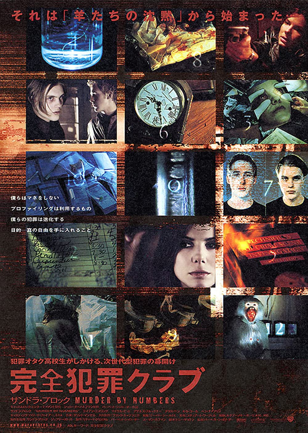
(a) drama,	(b) action,	(c) crime,	(d) action,
horror, mystery	sci-fi, –	mystery, thriller	adventure, fantasy

Figure 1: Example of movie posters with genres.

In Fig. 1, we present some movie poster samples with corresponding genres. Analyzing only poster images brings several challenges, since a single poster may have limited information (Fig. 1.(a)), intricate backgrounds (Fig. 1.(b)), incorporated multiple small images in a collage (Fig. 1.(c)), or included solely the cast member photos (Fig. 1.(d)). Here, we analyze only the poster image without any aid of other modalities to identify its genre, which is a considerably more challenging task compared to other computer vision tasks, e.g., object detection, scene recognition and classification. Unlike objects, genres are intangible implicit features that can hardly be precisely determined in a poster [1]. Here, genre identification depends on the individual human perception, i.e., a poster can belong to one genre for a person, and the same poster is of another genre to some other person. A movie poster may be of multiple genres, introducing the challenge of multi-label classification [9] and potentially exacerbating data imbalance concerns [10]. In a poster, a genre may be suppressed by other genres, e.g., in Fig. 1.(d), action and adventure genres are more explicit than fantasy. Moreover, the information present in posters itself brings additional challenges in identifying the movie genre, which we briefly mention in Appendix B. In this study, we obtained posters from IMDb, where each poster can be multi-labeled [9] with a maximum of three movie genres.

In this paper, we harness the power of a transformer-based architecture for its ability to grasp the global context and decipher intricate relationships spanning the entire poster image [11]. We first introduce a residual dense transformer, and then engage an ensemble mechanism and an asymmetric loss to tackle multi-label genre identification [12]. Furthermore, we propose a probabilistic module to accommodate a variable number of genres in the classification process. We now briefly mention our contributions to this paper.

(i) We work with genre identification only from poster images without any aid from textual/ video/ audio modalities. We introduce a residual dense transformer model, which features densely connected transformer encoders. Here, the model takes deep feature embeddings as input, instead of raw image patches.

(ii) A poster can often be associated with multiple movie genres, presenting a multi-label classification challenge. To effectively address this issue, we employ an ensemble technique. Additionally, we adopt an asymmetric loss function to handle the intricacies of multi-label classification, particularly when positive labels are less prevalent than negative ones.

(iii) Movie posters may exhibit a variable number of multi-genres. To adapt to this variability, we introduce a probabilistic module designed to eliminate extraneous genres and accurately discern the varying number of genres associated with each poster. To the best of our knowledge, this is the earliest attempt of its kind.

(iv) To assess the effectiveness of our model, we conducted comprehensive experiments on the poster images procured from IMDb, compared with contemporary architectures, and performed an ablation study. Our findings offer valuable insights into the interplay between poster visual elements and movie genres, benefiting film recommendation systems and the film industry’s digital evolution.

The rest of the paper is organized as follows. Section II provides a concise overview of related literature. The subsequent section III discusses the proposed methodology, followed by section IV, which delves into the analysis of experimental results. Finally, section V concludes this paper.

II Related Work

Our primary focus in this paper is identifying multi-label movie genres exclusively from posters. Using only posters as input for this task is relatively limited in the literature [1]. However, some past works used trailer [13], clips [14], and facial frames [5] as visual inputs. Additionally, numerous studies have focused on textual inputs, such as movie plot summary [6] / synopsis [15] and screenplay [16]. Furthermore, past research endeavors engaged multimodal approaches, combining visual, textual, and audio data as input [17, 18]. Now, we provide a brief summary of significant prior studies, in addition to Table I.

Visual Input: Visual data related to a movie, e.g., poster, teaser, trailer, or clip, can convey cues about the genre of the film. Many studies in the literature emphasized trailers [19, 13, 20, 4, 14], while only a few works have explored the use of movie posters [21, 8, 22, 1] for genre identification.

From a movie trailer, Zhou et al. [19] chose keyframes and extracted GIST, CENTRIST, and W-CENTRIST features, followed by a nearest neighbor (kNN)-based classifier to identify the movie genre. Simões et al. [13] employed a CNN (Convolutional Neural Network) model to detect 4 different genres within a selection of trailers procured from LMTD (Labeled Movie Trailer Dataset). Wehrmann et al.[20] also used a CNN leveraging trailer frames across time to detect 9 genres from some trailers of LMTD. In [4], genres were identified from trailer clips using DIViTA (Dual Image and Video Transformer Architecture). In [14], spatio-temporal features were extracted from video clips, followed by using a hSVM (hierarchical Support Vector Machine). Initially, the videos were categorized into broader categories, e.g., movie, news, sports, commercial, and music videos, after which the specific genre was identified. Yadav et al. [5] predicted emotions of facial frames of trailers followed by genre identification using an Inception-LSTM-based architecture.

Pobar et al. [21] used Naïve Bayes (NB) classifier on GIST and classeme features extracted from movie posters to predict the genres. In [8], YOLO was used to detect objects on posters and a CNN model was engaged for corresponding genre identification. Turkish movie genres were identified in [22] from posters using a basic CNN architecture. Wi et al. [1] employed a Gram layer to extract style features and merged with a CNN to classify genres from posters only.

TABLE I: Summary of related works for movie genre identification

Method Input Architecture/ #Genre/ Dataset Multi- Technique #Tags label? Visual [19] Trailer GIST, CENTRIST, kNN 4 ($\wp$) $\upchi$ [13] Trailer CNN 4 LMTD $\upchi$ [20] Trailer CNN 9 LMTD ✓ [4] Trailer Transformer 10 Trailers12k ✓ [14] Clip hSVM 4 ($\wp$) $\upchi$ [5] Facial frame Inception-LSTM 6 EmoGDB ($\wp$) ✓ [21] Poster NB 18 TMDb ($\wp$) ✓ [8] Poster CNN, YOLO 23 IMDb ($\wp$) ✓ [22] Poster CNN 4 ($\wp$) $\upchi$ [1] Poster CNN, Gram layer 12 IMDb ($\wp$) ✓ Ours Poster ERDT, PrERDT 13 IMDb ✓ 2 Textual [23] Plot summary BLSTM 4 ($\wp$) $\upchi$ [6] Plot summary GRU 20 IMDb ($\wp$) ✓ [15] Synopsis CNN-FE 71 MPST ✓ [24] Synopsis CNN, LSTM 9 MLMRD $\upchi$ [7] Synopsis Self-Attention 9 LMTD ✓ [16] Screenplay MLE, LSTM 31 Jinni ($\wp$) ✓ 2 Multimodal [17] Synopsis, Metadata, MulT-GMU 13 Moviescope ✓ Poster, Trailer, Audio ($\wp$) [18] Synopsis, Metadata, fastText, fastVideo, 13 Moviescope ✓ Poster, Trailer, Audio CRNN, VGG-16 ($\wp$) [25] Synopsis, Subtitle, Textural feature, LSTM 18 TMDb ($\wp$) ✓ Poster, Trailer, Audio kNN, SVM, MLP, DT [26] Synopsis, Metadata, Poster Word2Vec, CNN, GMU 23 MM-IMDb ✓ [27] Trailer, Audio Rule-based classifier 4 ($\wp$) $\upchi$ [28] Subtitle, Video DCT, BoW, SVM 18 ($\wp$) $\upchi$ ($\wp$): Publicly unavailable

Textual Input: Textual data in movies, including plots/ synopses, subtitles, and user-generated reviews on social media, offer valuable insights into genre identification.

Ertugrul et al. [23] employed BLSTM (Bidirectional Long Short-Term Memory) to classify movie genres based on sentences extracted from plot summaries. In [6], GRU (Gated Recurrent Unit) was for a similar input/output.

Kar et al. [15] engaged plot synopses and proposed CNN-FE (CNN with Flow of Emotions) encoded with emotion flow, CNN, and BLSTM to predict movie tags, i.e., genres and associated plot-related attributes (e.g., violence, suspenseful, melodrama). Battu et al. [24] identified genres from synopses of multi-language movies. They also attempted movie rating prediction. Multiple models based on CNN, LSTM, and GRU were used. In [7], CNN with a self-attention mechanism was used for genre classification from textual synopses.

Movie screenplays were engaged by Gorinski et al. [16] to predict various movie attributes, including genre, mood, plot, and style. They used a multi-label encoder (MLE) and LSTM-based decoder for this task.

Multimodal Input: In the past, often, two or more modalities (e.g., text, image, video, audio) were combined and used for the genre identification.

Arevalo et al. [26] proposed GMU (Gated Multimodal Unit) to fuse features extracted from text (synopsis, metadata) and image (poster) using Word2Vecc and CNN, respectively. Bribiesca et al. [17] engaged text (synopsis, metadata), image (poster), video (trailer), audio, and fed to MulT-GMU, which is a transformer architecture with GMU, to identify movie genres. Bonilla et al. [18] proposed a multi-modal fusion using fastText, fastVideo, VGG-16, CRNN to fuse text (plot, metadata), video (trailer), image (poster), audio, respectively, for movie genre identification. In [25], various textural features were extracted from the text (synopsis, subtitle), video (trailer), image (poster), audio, and fed to various classifiers, e.g., LSTM, kNN, SVM, MLP (Multi-Layer Perceptron), DT (Decision Tree) followed by a fusion step to classify genres. Rasheed [27] et al. computed average shot length, visual disturbance, audio energy from trailer video/ audio and used a rule-based classifier to classify into four genres. In [28], DCT (Discrete Cosine Transform) and BoW (Bag-of-Word) were used to extract features from trailer videos and subtitles, respectively, followed by SVM for detecting movie genres.

Positioning of our work: In the literature, there is a scarcity of research that focuses on genre identification exclusively from poster images. Furthermore, prior studies heavily leaned towards utilizing CNN-based features and did not effectively tackle the intricacies of multi-label genres. Our study is one of the earliest attempts to perform genre identification solely through poster images using a transformer-based architecture proficient in handling multi-label genres and eliminating extraneous genre labels.

III Proposed Methodology

In this section, we first formulate the problem and subsequently present the solution architecture.

III-A Problem Formulation

We are given:

1. A set of $\delta$ genres ${\cal{G}}=\{{\cal{G}}_{1},{\cal{G}}_{2},\ldots,{\cal{G}}_{\delta}\}$

2. A set of $n$ movie poster images ${\cal{I}}=\{{\cal{I}}_{1},{\cal{I}}_{2},\ldots,{\cal{I}}_{n}\}$

3. Each movie poster image ${\cal{I}}_{i}\in{\cal{I}}$ is associated with a set of $\kappa_{i}$ number of genres ${\cal{G}}^{<i>}=\{{\cal{G}}^{<i>}_{1},{\cal{G}}^{<i>}_{2},\ldots,{\cal{G}}^{<i>}_{\kappa_{i}}\}\subseteq{\cal{G}}$, $1\leq\kappa_{i}\leq\delta$

In this paper, we represent the ground-truth genre in terms of a multi-hot encoding vector (an example is shown in Fig. 2). The encoding of ${\cal{I}}_{i}$ is represented by $\Lambda^{<i>}$ of length $\delta$, as defined below:

$$\Lambda^{<i>}_{j}=\begin{cases}1~{},&~{}~{}\text{if ${\cal{I}}_{i}$ is associated with ${\cal{G}}_{j}$}\\ 0~{},&~{}~{}\text{otherwise}\end{cases}$$ (1)

Given an unknown movie poster ${\cal{I}}_{u}$, the objective here is to identify the genres associated with ${\cal{I}}_{u}$. Since a sample can have more than one positive class, we formulate this problem as a multi-label classification task [9], and predict multiple genre labels for each movie poster image.

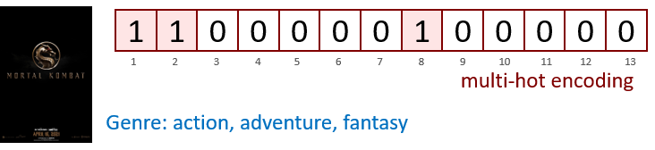
Figure 2: Multi-hot encoding of a movie poster genre.

III-B Solution Architecture

We employ a transformer network for our task due to its capacity for reducing inductive bias and its effectiveness in capturing global dependencies and contextual understanding compared to CNNs. However, it is important to note that in our approach, we do not directly utilize the ViT (Vision Transformer) paradigm, which involves feeding raw image patches directly into the transformer encoder [11]; instead, we feed deep feature embeddings and perform dense connection among the transformer encoders. We now begin with presenting our architecture, Residual Dense Transformer.

III-B1 Residual Dense Transformer (RDT)

RDT comprises three main modules: deep feature embedding, densely connected transformer encoders comprising multi-head self-attention and multi-layer perceptron, and a feed-forward neural network [29]. The pictorial representation of the workflow of RDT is shown in Fig. 3, and the modules are discussed below.

(i) Deep feature embedding: The transformer network takes input into a sequence of token embedding [29]. Here, the input image $\mathcal{I}_{o}$ is first resized into $\mathcal{I}\in\mathbb{R}^{w_{z}\times w_{z}\times c_{p}}$ that is converted into a sequence of patches $x_{p}^{i}\in\mathbb{R}^{w_{p}\times w_{p}\times c_{p}}$, for $i=1,2,\ldots,n_{p}$. From each patch $x_{p}^{i}$, we extract deep features $a_{p}^{i}$ using a convolutional architecture $f_{a}$. For our task, up to the average_pool layer of ResNet50V2 [30] as $f_{a}$ works better among some contemporary architectures [31]. The employed $f_{a}$’s share weights among patches. Empirically, we set $w_{z}=1024$, $w_{p}=256$, $n_{p}=(w_{z}/w_{p})^{2}=16$, and $c_{p}=3$ that denotes the RGB channel count of $\mathcal{I}$.

Further, each $a_{p}^{i}$ is flattened and mapped into a $D$-dimensional vector, i.e., embedding $z_{0}$ through transformer layers by the below linear projection.

$$z_{0}=\left[a_{class}~{};~{}a_{p}^{1}\operatorname{\mathbb{E}}~{};~{}a_{p}^{2}\operatorname{\mathbb{E}}~{};~{}\ldots~{};~{}a_{p}^{n_{p}}\operatorname{\mathbb{E}}\right]+\operatorname{\mathbb{E}}_{pos}$$ (2)

where, $\operatorname{\mathbb{E}}\in\mathbb{R}^{w_{p}\times w_{p}\times c_{p}\times D}$ is the patch embedding projection, $\operatorname{\mathbb{E}}_{pos}\in\mathbb{R}^{(n_{p}+1)\times D}$ is the positional encoding that holds the patches’ position information [32], and $a_{class}=z_{0}^{0}$ is a learnable embedding [11].

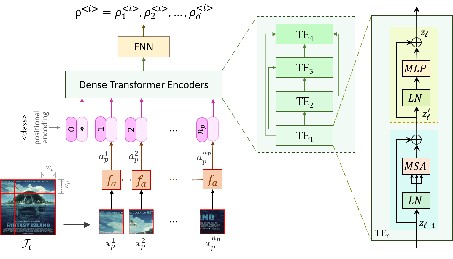
Figure 3: Workflow of Residual Dense Transformer (RDT)

(ii) Dense transformer encoders: After mapping the image patches to the deep feature embedding space with positional encoding, we employ densely connected transformer encoders sequentially [32]. Here, the $\ell^{th}$ transformer encoder (TE_ℓ) inputs concatenated feature encodings ($\mathcal{X}$) of all preceding encoders:

$$\mathcal{X}(\text{TE}_{\ell})=\left[\mathcal{X}(\text{TE}_{1});\mathcal{X}(\text{TE}_{2});\ldots;\mathcal{X}(\text{TE}_{\ell-1})\right]$$ (3)

The building blocks of a TE are shown in Fig. 3, which includes alternating layers of $MSA$ (Multi-head Self-Attention) and $MLP$ (Multi-Layer Perceptron) blocks [11, 33].

Multi-head Self-Attention ($MSA$)

The core of the TE is its $MSA$ mechanism consisting of $h$ parallel attention layers, i.e., attention heads, where each head utilizes SA (Scaled dot-product Attention) [32]. The SA takes input comprising $D_{K}$ dimensional queries and keys, and $D_{V}$ dimensional values [32], and computed as follows.

$$SA(Q,K,V)=softmax\left({QK^{T}}\diagup{\sqrt{D_{K}}}\right)V$$ (4)

where, a set of queries, keys, and values are packed to form $Q$, $K$, $V$ matrices, respectively.

$MSA$ empowers the capability to focus on information across diverse representations at various positions. Here, concurrent self-attention computations for each head collectively output as below.

$$\centering\begin{split}MSA(Q,K,V)=\left[head_{1},head_{2},\ldots,head_{h}\right]W_{O};\\ head_{i}=SA(QW_{i}^{Q},KW_{i}^{K},VW_{i}^{V})\end{split}\@add@centering$$ (5)

where, $W_{i}^{Q}\in\mathbb{R}^{D\times D_{K}}$, $W_{i}^{K}\in\mathbb{R}^{D\times D_{K}}$, $W_{i}^{V}\in\mathbb{R}^{D\times D_{V}}$, $W_{O}\in\mathbb{R}^{hD_{V}\times D}$ are parameter matrices; $D_{K}=D_{V}=\lfloor D/h\rfloor$.

Multi-Layer Perceptron ($MLP$)

The $MLP$ block consists of two fully connected layers with $2D$ and $D$ nodes, respectively, and employs the GELU (Gaussian Error Linear Unit) non-linear activation function, similar to [11].

Before and after the $MSA$ / $MLP$ blocks, $LN$ (Layer Normalization) [34] and residual connections [30] are engaged, respectively (Fig. 3). It can be represented as below.

$$\begin{split}z_{\ell}=MLP(LN(z^{\prime}_{\ell}))+z^{\prime}_{\ell};\\ z^{\prime}_{\ell}=MSA(LN(z_{\ell-1}))+z_{\ell-1};~{}\ell=1,2,\ldots,L\end{split}$$ (6)

where, $L$ is the total count of engaged TEs. After multiple TEs, the <class> token is imbued with contextual information. The learnable embedding state at the outcome of the TE_L, i.e., $z_{L}^{0}$, serves as the image representation $y^{\prime}$ [11]; $y^{\prime}=LN(z_{L}^{0})$.

(iii) Feed-forward neural network (FNN): The final stage of our model comprises an FNN consisting of one hidden layer with $D/2$ nodes having ReLU activation function [33], followed by an output layer. The output layer contains $\delta$ number of nodes with sigmoid as output function [33]. To mitigate the challenge in multi-label classification, where positive labels are lesser than negative ones, we leverage the asymmetric loss function (ASL) to train our model [12]. We use Adam optimizer here due to its adaptive learning rates and efficient memory usage [35].

Finally, for a poster image ${\cal{I}}_{i}$, RDT generates a confidence score vector ${\uprho^{<i>}}=(\rho_{1}^{<i>},\rho_{2}^{<i>},\ldots,\rho_{\delta}^{<i>})$. The top-3 genres based on the confidence scores are selected as the associated genres of ${\cal{I}}_{i}$.

III-B2 Ensmebled Residual Dense Transformer (ERDT)

Given that data imbalances are a common issue in multi-label classification problems [9], here, we propose an ensemble strategy to mitigate this challenge. In our proposed ensemble method, we consider three fundamental models: (a) R: the residual network with sigmoid as the output function and ASL as the loss function, (b) RT: the residual transformer network, a simplified version of the RDT that does not include dense connections, (c) RDT: the proposed model.

For a poster ${\cal{I}}_{i}$, we first obtain three confidence score vectors ${\uprho_{i,1}}=(\rho_{1}^{<i,1>},\rho_{2}^{<i,1>},\ldots,\rho_{\delta}^{<i,1>})$, ${\uprho_{i,2}}=(\rho_{1}^{<i,2>},\rho_{2}^{<i,2>},\ldots,\rho_{\delta}^{<i,2>})$, and ${\uprho_{i,3}}=(\rho_{1}^{<i,3>},\rho_{2}^{<i,3>},\ldots,\rho_{\delta}^{<i,3>})$ from R, RT, and RDT models, respectively, which are then combined using weighted mean ensemble scheme [36], as shown in Eq. 7, to produce the confidence score vector ${\uprho_{i}}=(\rho_{1}^{<i>},\rho_{2}^{<i>},\ldots,\rho_{\delta}^{<i>})$ for the ERDT model.

$$\centering\rho_{j}^{<i>}={\sum\limits_{k=1}^{3}\alpha_{k}~{}\rho_{j}^{<i,k>}};~{}~{}\forall j\in\{1,2,\ldots,\delta\}\@add@centering$$ (7)

where, $0\leq\alpha_{k}\leq 1$; ${\sum\limits_{k=1}^{3}\alpha_{k}}=1$; for $k=1,2,3$ represents the weights that were tuned by a grid-search technique [37].

III-B3 Probabilistic Module

As discussed earlier, a movie poster can encompass multiple genres. Given an input poster ${\cal{I}}_{i}$, the multi-label classifier generates a confidence score vector $\uprho_{i}=(\rho_{1}^{<i>},\rho_{2}^{<i>},\ldots,\rho_{\delta}^{<i>})$ of ${\cal{I}}_{i}$ comprising the confidence score for each genre to be associated with ${\cal{I}}_{i}$. The top three genres with the highest confidence score are predicted as the associated genres with ${\cal{I}}_{i}$. However, the poster can be associated with fewer than three genres. To address this issue, here, we propose a probabilistic module. The objective of this module is to determine whether the poster is associated with more than one genre and, if so, select the 2^nd and 3^rd genres accordingly.

The crux of this module is to compute the association between genres, which are captured by the following equations.

$$P(g_{k}|g_{j})={|{\cal{Z}}_{j}\cap{\cal{Z}}_{k}|}~{}/~{}{|{\cal{Z}}_{j}|}$$ (8)

$$P(g_{l}|g_{j},g_{k})={|{\cal{Z}}_{j}\cap{\cal{Z}}_{k}\cap{\cal{Z}}_{l}|}~{}/~{}{|{\cal{Z}}_{j}\cap{\cal{Z}}_{k}|}$$ (9)

where, ${\cal{Z}}_{j}$ is the set of posters that are associated with genre ${\cal{G}}_{j}$. Eqn. 8 expresses the likelihood of a poster being associated with ${\cal{G}}_{k}$, considering that the poster is already associated with ${\cal{G}}_{j}$. Eqn. 9 denotes the probability of a poster being associated with ${\cal{G}}_{l}$, given that the poster is already associated with both ${\cal{G}}_{j}$ and ${\cal{G}}_{k}$. We calculate the conditional probabilities in advance for all possible combinations of genres.

Once the multi-label classifier generates the confidence score vector $\uprho_{i}$ for the input poster ${\cal{I}}_{i}$, the genre with the highest confidence score is chosen to be the first genre of ${\cal{I}}_{i}$. We refer to this first genre as the dominant genre.

The 2^nd genre of ${\cal{I}}_{i}$ is determined based on the dominant genre. Let us assume that ${\cal{G}}_{j}$ is the dominant genre for ${\cal{I}}_{i}$ (i.e., ${\cal{G}}^{<i>}_{1}={\cal{G}}_{j}$). The 2^nd genre for ${\cal{I}}_{i}$ is selected by Eqn. 10.

$$\begin{split}{\cal{G}}^{<i>}_{2}=\underset{k\neq j,~{}1\leq k\leq\delta}{\arg\!\max}\left(\rho_{k}^{<i>}\times{\widetilde{P}}(g_{k}|g_{j})\right);\\ \text{if }\underset{k\neq j,~{}1\leq k\leq\delta}{\max}\left(\rho_{k}^{<i>}\times{\widetilde{P}}(g_{k}|g_{j})\right)>\tau\end{split}$$ (10)

where, $\widetilde{P}(g_{k}|g_{j})$ is the normalized probability value computed over $\left(P(g_{1}|g_{j}),P(g_{2}|g_{j}),\ldots,P(g_{\delta}|g_{j})\right)$, and $\tau$ is a tunable threshold determined empirically.

Here, for each genre other than $G_{j}$, an association score is computed. The association score for genre $G_{k}$ is determined by multiplying its confidence score $\rho_{k}^{<i>}$ with its normalized conditional probability value ${\widetilde{P}}(g_{k}|g_{j})$, provided that ${\cal{I}}_{i}$ is linked to $G_{j}$. If the maximum association score across all genres except $G_{j}$ exceeds a predefined threshold $\tau$, the corresponding genre is assigned in ${\cal{G}}^{<i>}_{2}$.

If the 2^nd genre of ${\cal{I}}_{i}$ (assuming ${\cal{G}}^{<i>}_{2}={\cal{G}}_{k}$) is chosen, we then proceed to determine whether to select the 3^rd genre. The selection of the 3^rd genre of ${\cal{I}}_{i}$ is captured by Eqn. 11.

$$\small\begin{split}{\cal{G}}^{<i>}_{3}=\underset{l\neq j,~{}l\neq k,~{}1\leq l\leq\delta}{\arg\!\max}\left(\rho_{l}^{<i>}\times{\widetilde{P}}(g_{l}|g_{j})\times{\widetilde{P}}(g_{l}|g_{j},g_{k})\right);\\ \text{if }\underset{l\neq j,~{}l\neq k,~{}1\leq l\leq\delta}{\max}\left(\rho_{l}^{<i>}\times{\widetilde{P}}(g_{l}|g_{j})\times{\widetilde{P}}(g_{l}|g_{j},g_{k})\right)>\tau^{\prime}\end{split}$$ (11)

where, $\widetilde{P}(g_{l}|g_{j},g_{k})$ represents normalized probability calculated from $\left(P(g_{1}|g_{j},g_{k}),P(g_{2}|g_{j},g_{k}),\ldots,P(g_{\delta}|g_{j},g_{k})\right)$, and $\tau^{\prime}$ is a tunable threshold, set empirically.

It is important to emphasize that selecting the 2^nd and 3^rd genres is greatly influenced by the correct prediction of the dominant genre. Therefore, an incorrect prediction for the dominant genre may lead to the inaccurate selection of the 2^nd and 3^rd genres.

In our experimental analysis, we show the performance of this probabilistic module with respect to the correct prediction of the dominant genre, which is denoted by hit ratio (${\cal{H}}it$) as defined below: ${\cal{H}}it={|TD_{c}|}~{}\diagup~{}{|TD|}$ where, $TD_{c}$ is the set of test samples for which the dominant genre is correctly identified, and $|TD|$ is the total number of employed test samples.

Finally, we integrate this probabilistic module with ERDT to obtain our final proposed model, PrERDT.

IV Experiments and Discussion

This section describes the employed dataset and experimental results with discussions.

IV-A Employed Dataset

TABLE II: Poster and movie counts across genre labels

Class Id	Genre label	Poster count	Movie count
1	Action	4985	1426
2	Adventure	3702	1024
3	Animation	1196	325
4	Biography	1076	348
5	Comedy	4380	1517
6	Crime	3052	1003
7	Drama	6609	2217
8	Fantasy	1379	423
9	Horror	2646	860
10	Mystery	2285	750
11	Romance	2406	913
12	Sci-Fi	1542	458
13	Thriller	3455	1092

The primary objective of this study is to analyze the poster images to identify their multi-labeled movie genres. Consequently, obtaining a dataset featuring posters with multiple genres proved challenging, as there were scarce off-the-shelf options available. Therefore, we procured authentic movie poster images with corresponding genres from Internet Movie Database (IMDb: https://developer.imdb.com/non-commercial-datasets). A movie may be of multiple genres; however, on IMDb, a maximum of 3 genres are labeled for an individual movie. Currently, our dataset considers 13 distinct genres (i.e., $\delta=$ 13), as mentioned in Table II. The ground-truth genre of a movie poster is available in terms of multi-hot encoding (refer to section III-A). We gathered posters of 4464 individual movies, each with 1 to 5 posters; the distribution of movie count with respect to the individual poster count is presented in Fig. 4.(a). Overall, our dataset comprises 13882 distinct posters, each having 1 to 3 genre labels. The movie and poster counts with respect to genre label count are shown in Fig. 4.(b). Here, we can see that about $\frac{3}{4}^{th}$ posters/movies of our dataset have 3 genre labels. For individual genre label/ class id, the corresponding poster and movie counts are shown in Table II. As a matter of fact, in this table, some poster/movie counts overlap across genres due to having multi-label genres. Here, genre drama is included in the highest number of posters, i.e., 6609; whereas biography has 1076 posters, which is the lowest in our dataset. Table II comprehends the data imbalance issue [10]. In Fig. C.1 (refer to Appendix B), we present some poster images from our employed dataset along with the genre class numbers. Fig. A.1 of Appendix A illustrates a co-occurrence matrix for movie genre labels associated with the posters.

From IMDb, while selecting the movies/poster, we followed the following strategies:

• sorted out movies based on release year since 2000.

• picked movies having more than 10000 user votes and more than 60 minutes of runtime.

• crawled and filtered movies based on the 13 genres employed here (refer to Table II).

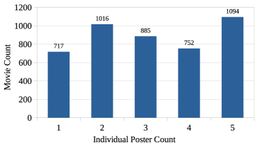
(a) (b)

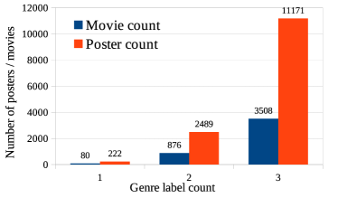
Figure 4: (a) Distribution of movie count w.r.t. individual poster count, (b) Distribution of movie & poster count w.r.t. genre-label count.

The dataset was split up into training ($DB_{tr}$), validation ($DB_{v}$), and testing ($DB_{t}$) disjoint sets with an approx ratio of $8:1:1$ considering the presence of all 13 genres in each set equivalently. $DB_{tr}$, $DB_{v}$, and $DB_{t}$ contain 10942, 1470, and 1470 posters, respectively.

IV-B Experimental Details

We executed the experimentation using the TensorFlow-2.5 framework having Python 3.9.13 on an Ubuntu 20.04.2 LTS-based machine with specifications including AMD EPYC 7552 Processor running at 2.20 GHz with 48 CPU cores and 256 GB RAM, NVIDIA A100-PCIE GPU with 40 GB of memory. In this paper, all the presented results were obtained from $DB_{t}$.

The hyper-parameters of our model were tuned and set during the model training with a focus on optimizing performance over $DB_{v}$. For the transformer networks, we fixed the following hyper-parameters empirically: transformer_layers ($L$) = 4, embedding_dimension ($D$) = 256, num_heads ($h$) = 6. In ASL, we set focusing parameters $\gamma^{+}=0$, $\gamma^{-}=1$, and probability margin $m=0.2$. For Adam optimizer, we chose initial_learning_rate = $10^{-3}$; exponential decay rates for 1^st and 2^nd moment estimates, i.e., $\beta 1=0.9$, $\beta 2=0.999$; zero-denominator removal parameter ($\upvarepsilon$) = $10^{-8}$. For the early stopping strategy, we set the patience parameter to 10 epochs, and we maintained a fixed mini-batch size of 32. We empirically chose $\tau=0.3$ and $\tau^{\prime}=0.03$ for our probabilistic module (refer to Eqn.s 10, 11).

We evaluated the model performance based on the macro-level analysis, considering standard metrics in multi-label classification, such as precision ($\cal{P}$) %, recall ($\cal{R}$) %, specificity (${\cal{S}}p$) %, balanced accuracy (${\cal{BA}}$) %, F-measure (${\cal{FM}}$) %, and Hamming loss (${\cal{HL}}$) [38].

IV-C Comparison with State-of-the-Art (SOTA) Models

TABLE III: Comparison with baseline and SOTA models

Method $\cal{P}$ $\cal{R}$ ${\cal{S}}p$ ${\cal{BA}}$ ${\cal{FM}}$ ${\cal{HL}}$ Baseline ResNet50V2 [30] 52.04 50.44 85.36 67.90 48.97 0.18524 DenseNet121 [39] 26.10 27.18 78.62 52.90 22.63 0.30120 EfficientNetB2 [40] 51.37 52.53 85.95 69.24 51.40 0.18503 ViT [11] 29.11 27.40 78.61 53.01 22.58 0.25243 InceptionV3 [41] 21.03 28.80 79.12 53.96 22.43 0.25599 MobileNetV2 37.34 33.22 80.57 56.90 30.37 0.23799 Improvement of RDT 2.97 4.72 1.13 2.93 4.29 7.75% Improvement of ERDT 3.91 5.35 1.40 3.38 5.00 10.58% Improvement of PrERDT 5.73 2.12 2.76 2.44 3.86 12.36% SOTA Chu et al. [8] 19.73 27.32 - - 20.89 - Gozuacik et al. [22] 36.76 35.12 80.91 58.02 33.49 0.24290 Pobar et al. [21] 28.76 47.76 68.18 57.97 34.72 0.34688 Wi et al. [1] 52.89 51.18 - - 49.61 - Improvement of RDT 2.12 6.07 6.17 14.15 6.08 29.73% Improvement of ERDT 3.06 6.70 6.44 14.60 6.79 31.88% Improvement of PrERDT 4.88 3.47 7.80 13.66 5.65 33.24% Proposed RDT 55.01 57.25 87.08 72.16 55.69 0.17069 ERDT 55.95 57.88 87.35 72.61 56.40 0.16546 PrERDT 57.77 54.65 88.71 71.68 55.26 0.16216

Table III presents the performance of the three models: RDT, ERDT and PrERDT, proposed in this paper. Here, we compare the performance of our proposed models with some major contemporary deep architectures, called baseline, and some related SOTA models. It may be noted the baseline models are designed for multi-class classification problems [31], and are typically not well-suited for handling multi-label classification challenges. Therefore, we improvised the baseline models by incorporating sigmoid as the output function and ASL as the loss function (refer to section III-B) to enable them to address multi-label classification. As evident from Table III, all three models, RDT, ERDT and PrERDT, outperformed the baseline models and SOTA in terms of all the performance evaluation metrics employed in this paper.

IV-D Ensemble Study

TABLE IV: Performance by various models for ensemble analysis

Model $\cal{P}$ $\cal{R}$ ${\cal{S}}p$ ${\cal{BA}}$ ${\cal{FM}}$ ${\cal{HL}}$ R 52.04 50.44 85.36 67.90 48.97 0.18524 RT 52.54 55.53 86.67 71.10 53.57 0.17833 RDT 55.01 57.25 87.08 72.16 55.69 0.17069 R + RT 54.76 56.28 87.04 71.66 54.69 0.16902 R + RDT 55.35 56.46 86.97 71.72 55.20 0.16954 RT + RDT 54.96 57.44 87.28 72.36 55.70 0.16755 ERDT 55.95 57.88 87.35 72.61 56.40 0.16546

Table IV presents the performance of various models participating in the ensemble. From this table, we have the following observations:

(i) Overall performance of ERDT: ERDT outperformed all other models listed in the first column of Table IV.

(ii) Comparison between RDT and R+RT: It is worth noting that the overall performance of the RDT was better than the R+RT model in terms of balanced accuracy and F-measure.

(iii) Comparison between RDT and R+RDT: As evident from Table IV, the performance of R+RDT is degraded compared to that of RDT in terms of balanced accuracy and F-measure. From Table VIII.(b), the reason for this can be explained. Table VIII.(b) shows the rank of each model based on the balanced accuracy for all 13 genres separately. According to these ranks, RDT performed better than R in all 13 genres. The negative influence of R caused the degradation of the performance of the R+RDT model in 8 out of 13 cases, which was reflected further in the overall performance of the R+RDT model across all genres.

(iv) Significance of the participating models in the ensemble: As per the ranking shown in Table VIII.(b), RT performed better than RDT for two genres (i.e., mystery, and sci-fi). Hence, we first choose to combine RT and RDT to improve the overall performance of RDT. Our experimental results show that in 6 of 13 genres, RT+RDT, indeed, performed better than RT and RDT individually. RT+RDT also outperformed RT and RDT independently in terms of overall performance across all genres. Furthermore, as per our observation from Table VIII.(b), for a few genres (e.g., adventure, animation, thriller), the overall performances of R, RT, and RDT are comparable. Hence, we select R, RT, and RDT as the fundamental models for our ensemble. It may be noted from Table VIII.(b) that in 6 out of 13 genres, ERDT performed better than RT+RDT. Moreover, in 5 out of the 8 cases for which R+RDT performed worse than RDT, the ERDT model performed better than RDT due to the influence of RT. In terms of the overall performance, ERDT also turned out to be the best, comparing all the fundamental models used for our ensemble and their other possible combinations. This justifies our choice of fundamental models for the ensemble. In Fig. C.2 of Appendix C, we show the qualitative performance of ERDT using heat map encoding.

IV-E Genre-wise Analysis

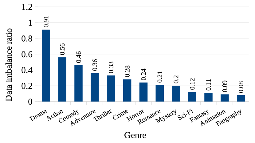
Figure 5: Genre-wise data imbalance ratio

According to Table IV, we have evaluated the models based on their balanced accuracy (and F-measure), resulting in the following ranking: ERDT $\succ$ RT+RDT $\succ$ RDT $\succ$ R+RDT $\succ$ R+RT $\succ$ RT $\succ$ R. Here, the notation Model-A $\succ$ Model-B indicates that the balanced accuracy of Model-A surpasses that of Model-B. Here, we perform a detailed analysis of the models’ performance across different genres, focusing on balanced accuracy. Table VIII.(a) provides a breakdown of the genre-wise performance analysis for all the models. From this table, we have yielded the following noteworthy findings:

(i) Comparison among fundamental models: RT demonstrated superior performance when compared to R in 12 out of 13 genres, highlighting its improvement over the latter. Similarly, RDT, being an enhancement over RT, outperformed RT in 11 out of 13 genres.

(ii) Comparison between the proposed fundamental model with other ensemble models: RDT outperformed R+RT in 7 out of 13 genres. We observed performance improvements for the R+RDT and RT+RDT models over the RDT model in 5 and 8 of the 13 genres, respectively. The ERDT model performed better than the RT+RDT model in 6 of 13 genres. Interestingly, despite the RT+RDT model outperforming ERDT in more genres when considering the count, the quantitative measure of improvement for ERDT was significantly higher than the degradation observed for ERDT in all the genres where RT+RDT surpassed the ERDT model.

(iii) Performance of R, RDT, and ERDT on imbalanced genres: Fig. 5 represents the ratio between positive and negative samples for each genre. This figure clearly illustrates that certain genres, such as biography, animation, and fantasy, suffer from significant data imbalance issues. Here, our analysis focuses on evaluating the performance of R, RDT, and ERDT specifically for these imbalanced genres. Fig. 6 visually depicts the comparative performance of these models in terms of specificity and recall for the biography and fantasy genres, both of which exhibit high levels of data imbalance. As observed in Fig.s 6 (a) and (b), the specificity performance of R is notably high, while its recall performance is considerably low in these imbalanced genres. This indicates that R struggles to address the challenge posed by imbalanced data effectively since R is unable to identify the posters belonging to these genres. In contrast, the RDT model performed better by identifying more posters from the imbalanced genres compared to the R model, resulting in improved recall. However, this gain in recall came at the cost of reduced specificity. The trade-off between recall and specificity is observed for the ERDT model. In other words, ERDT exhibits higher specificity compared to RDT but lower than R. Additionally, ERDT demonstrates higher recall compared to R but lower than RDT. As a result, the balanced accuracy of the ERDT model surpasses that of both the R and RDT models.

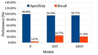
(a) (b)

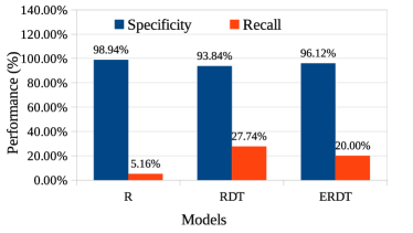
Figure 6: Comparative performance of R, RDT, and ERDT for imbalanced genres: (a) Biography, (b) Fantasy.

IV-F Ablation Study

TABLE V: Ablation Study

Model $\cal{P}$ $\cal{R}$ ${\cal{S}}p$ ${\cal{BA}}$ ${\cal{FM}}$ ${\cal{HL}}$ R 52.04 50.44 85.36 67.90 48.97 0.18524 T 29.11 27.40 78.61 53.01 22.58 0.25243 RT 52.54 55.53 86.67 71.10 53.57 0.17833 DT 33.78 29.81 79.14 54.48 25.42 0.26509 RDT 55.01 57.25 87.08 72.16 55.69 0.17069 R + RDT 55.35 56.46 86.97 71.72 55.20 0.16954 RT + RDT 54.96 57.44 87.28 72.36 55.70 0.16755 ERDT 55.95 57.88 87.35 72.61 56.40 0.16546 PrERDT 57.77 54.65 88.71 71.68 55.26 0.16216

Table V shows the ablation study of our proposed architecture. The observation from this table is listed below:

(i) Ablation study for RDT: As discussed earlier, RDT is the composition of a residual network and dense transformer. Therefore, here, we first compare the performance of RDT with other component models, such as the Residual network (R), Transformer network (T), Dense Transformer (DT), and Residual Transformer network (RT). As evident from Table V, RDT outperformed R, T, RT, and DT. This comprehends the impact of our proposed fundamental model RDT.

(ii) Incremental performance improvement due to improvisation of the models: It is worth noting from Table V that as RT is an improvisation over R and T individually, the performance of RT is better than each of R and T. Similarly, as DT is an improvisation over T, the performance of DT is better than T. Finally, RDT is an improvisation over RT and DT models; therefore, the performance of RDT is better than them.

(iii) Ablation study for ERDT: Table V shows that our ensemble model ERDT performed better than any other combination of the fundamental models (i.e., R, RT, and RDT) used in the proposed ensemble.

The analysis for PrERDT is presented next.

IV-G Analysis of Probabilistic Module

Figure 7: Performance analysis on hit ratio $({\cal{H}}it)$.

The last row of Table V shows the performance of PrERDT. It may be noted when we used the probabilistic module on ERDT, i.e., for the PrERDT model, the recall decreased more than the improvement in the precision and specificity (refer to the last two rows of Table V). Consequently, the balanced accuracy and the F-measure were decreased for PrERDT. However, the motivation for introducing the probabilistic module is to enhance precision while making only minimal concessions in recall, ultimately leading to improved balanced accuracy and the F-measure. The reason behind obtaining the counterintuitive outcome can be elucidated by referring to Fig. 7. The performance of our probabilistic module highly relies on accurately identifying the first genre through ERDT. However, according to Fig. 7, the hit ratio of the ERDT model for identifying the first genre is 0.7701. Consequently, the PrERDT model sometimes discarded the correctly predicted second and third genres due to its dependency on the erroneously predicted first genre, thus causing a decline in recall.

To validate the correctness of our hypothesis, we conducted an additional experiment on different subsets of test data where the hit ratio is notably high. Table VI shows the performance of our probabilistic module for five different subsets of test data characterized by a high hit ratio. As observed from Table VI, the precision for the PrERDT model exhibited improvement when compared to the ERDT model without compromising the recall value. Consequently, this enhancement translated into improved balanced accuracy and F-measure metrics for the PrERDT model. These findings underscore the effectiveness of our probabilistic module.

TABLE VI: Significance of the probabilistic module

Model ${\cal{H}}it$ $\cal{P}$ $\cal{R}$ ${\cal{S}}p$ ${\cal{BA}}$ ${\cal{FM}}$ ${\cal{HL}}$ ERDT 0.8889 79.48 91.78 95.60 93.69 84.27 0.04102 PrERDT 80.17 91.78 95.70 93.74 84.64 0.04017 ERDT 0.9000 87.25 96.44 95.84 96.14 91.08 0.03760 PrERDT 87.74 96.44 95.94 96.19 91.38 0.03675 ERDT 0.9111 87.81 87.28 95.86 91.57 85.72 0.03760 PrERDT 87.94 87.28 96.05 91.66 85.79 0.03675 ERDT 0.9133 84.70 92.51 95.73 94.12 88.10 0.03880 PrERDT 84.94 92.51 95.77 94.14 88.23 0.03846 ERDT 0.9444 83.49 92.82 94.46 93.64 86.21 0.04444 PrERDT 84.78 92.82 94.54 93.68 87.24 0.04358

IV-H Performance Analysis based on Genre Label Count

TABLE VII: Performance study (${\cal{BA}}$ %) on genre label count

$TD^{<1>}$ $TD^{<2>}$ $TD^{<3>}$ Model w/o Pr Pr w/o Pr Pr w/o Pr Pr R 50.68 50.70 63.88 62.70 67.87 66.79 RT 48.67 49.09 68.08 68.29 70.93 70.13 RDT 50.73 51.31 69.57 66.61 72.07 70.86 R + RT 49.45 49.08 67.90 66.95 71.60 70.46 R + RDT 50.70 51.62 68.24 65.05 71.28 70.14 RT + RDT 49.87 49.73 69.20 68.61 72.20 71.37 ERDT 51.58 49.36 70.26 69.69 72.34 71.41 $TD^{<k>}$: Test data with posters associated with $k$ number of genres

As mentioned earlier in section IV-A and shown in Fig. 4.(b), each poster in our dataset is associated with either 1, 2, or 3 genre labels. In this experiment, we partitioned the test data into three subsets with posters associated with 1, 2, and 3 genres, and present the results in Table VII. From Table VII, it can be comprehended that posters having 3 genres yielded the best performance. Here also, in most of the cases, ERDT demonstrated the best performance.

TABLE VIII: Genre-wise performance analysis and ranking of the models

(a) Genre-wise performance study Genre Action Adventure Animation Biography Comedy Crime Drama Fantasy Horror Mystery Romance Sci-Fi Thriller Model w/o Pr Pr w/o Pr Pr w/o Pr Pr w/o Pr Pr w/o Pr Pr w/o Pr Pr w/o Pr Pr w/o Pr Pr w/o Pr Pr w/o Pr Pr w/o Pr Pr w/o Pr Pr w/o Pr Pr $\cal{P}$ R 65.86 68.86 66.26 68.72 86.76 90.44 21.05 18.18 59.69 60.59 46.28 47.12 56.83 57.51 36.36 40.00 50.18 59.46 40.58 45.28 48.25 48.89 55.79 58.75 42.58 45.50 RT 75.22 76.09 67.47 69.67 87.12 89.81 18.27 22.35 66.17 66.81 46.11 47.45 63.17 63.30 29.33 39.54 58.94 61.11 35.97 35.75 45.10 46.28 44.50 48.00 45.71 47.16 RDT 76.03 77.49 76.01 78.10 85.29 86.79 25.96 29.11 67.99 68.40 46.33 47.71 61.62 62.44 34.68 33.75 54.60 62.34 33.50 35.80 49.59 50.00 54.55 59.62 48.95 48.23 R + RT 74.75 76.10 69.55 70.91 89.24 90.39 19.44 16.67 66.67 67.17 48.80 48.22 62.01 62.66 38.30 46.43 59.32 64.21 38.22 41.21 50.43 50.65 48.33 52.94 46.84 48.62 R + RDT 75.04 76.74 75.60 77.18 86.67 87.58 27.85 29.51 66.31 66.23 45.61 46.44 60.32 61.06 37.35 36.00 54.52 61.23 35.64 38.04 49.58 50.00 56.25 60.19 48.86 50.00 RT + RDT 76.40 78.14 71.68 72.82 86.39 87.81 22.68 23.38 67.22 67.25 49.27 49.69 62.83 63.00 35.14 45.65 58.97 65.42 36.32 37.98 48.78 49.38 49.15 55.40 49.59 50.29 ERDT 75.97 77.84 73.72 73.42 87.95 87.20 24.21 24.32 68.03 66.74 48.38 50.32 61.80 63.36 37.81 47.27 58.39 65.30 36.57 36.45 48.96 49.58 53.29 57.14 52.24 52.10 R 72.83 67.77 66.67 61.93 79.88 75.00 3.67 1.84 75.49 74.27 44.77 42.81 87.69 86.00 5.16 2.58 52.99 32.84 26.17 22.43 57.90 57.90 28.65 25.41 53.80 45.38 RT 68.09 66.35 75.10 73.25 86.59 85.98 17.43 17.43 75.97 73.79 52.29 48.69 77.85 77.23 14.19 10.97 54.10 45.15 42.52 39.25 60.53 58.95 52.43 45.41 44.84 42.94 RDT 69.67 65.25 69.75 67.49 88.42 84.15 24.77 21.10 74.76 73.54 53.60 50.98 85.23 84.92 27.74 17.42 66.42 53.73 31.31 29.44 63.16 63.16 38.92 33.51 50.54 44.29 R + RT 72.04 68.40 76.13 72.22 85.98 85.98 12.84 7.34 78.64 75.49 53.27 48.69 83.39 82.62 11.61 8.39 58.21 45.52 40.19 38.32 62.11 61.58 47.03 38.92 50.27 47.83 R + RDT 71.72 67.77 71.40 67.49 87.20 85.98 20.18 16.51 75.49 73.79 50.98 49.02 87.23 86.62 20.00 11.61 65.30 51.87 31.31 28.97 62.11 62.11 38.92 33.51 52.17 46.74 RT + RDT 71.09 68.88 75.51 72.22 89.02 87.81 20.18 16.51 78.16 75.24 55.23 51.96 83.23 82.00 16.77 13.55 60.08 52.24 37.85 36.92 63.16 63.16 47.03 41.62 49.46 46.47 $\cal{R}$ ERDT 70.93 68.25 73.87 71.61 89.02 87.20 21.10 16.51 76.94 74.52 53.60 51.96 85.39 83.54 20.00 16.77 64.93 53.36 36.92 34.58 62.11 61.58 43.78 43.24 53.80 47.28 ${\cal{S}}p$ R 71.45 76.82 83.23 86.08 98.47 99.00 98.90 99.34 80.15 81.19 86.34 87.37 47.20 49.63 98.94 99.54 88.27 95.01 93.47 95.38 90.78 91.02 96.73 97.43 75.77 81.85 RT 83.03 84.23 82.11 84.25 98.39 98.77 93.75 95.15 84.88 85.73 83.93 85.82 64.02 64.51 95.97 98.02 91.60 93.59 87.10 87.98 89.06 89.84 90.58 92.92 82.21 83.94 RDT 83.39 85.66 89.13 90.65 98.09 98.39 94.34 95.89 86.29 86.77 83.68 85.31 57.93 59.51 93.84 95.97 87.69 92.76 89.41 91.00 90.47 90.63 95.33 96.73 82.40 84.12 R + RT 81.60 83.75 83.54 85.37 98.70 98.85 95.74 97.06 84.69 85.63 85.31 86.25 59.51 60.98 97.79 98.86 91.10 94.34 88.93 90.68 90.94 91.09 92.76 95.02 80.94 83.12 R + RDT 81.96 84.47 88.52 90.04 98.32 98.47 95.81 96.84 85.07 85.35 83.93 85.14 54.51 56.22 96.12 97.57 87.85 92.68 90.45 91.96 90.63 90.78 95.64 96.81 81.76 84.39 RT + RDT 83.39 85.42 85.26 86.69 98.24 98.47 94.49 95.66 85.16 85.73 85.05 86.17 60.98 61.83 96.35 98.10 90.68 93.84 88.69 89.73 90.16 90.39 93.00 95.18 83.21 84.66 R + RT + RDT 83.03 85.30 86.99 87.20 98.47 98.39 94.71 95.89 85.92 85.54 84.97 86.51 58.17 61.71 96.12 97.79 89.68 93.68 89.09 89.73 90.39 90.70 94.47 95.33 83.58 85.48 R 72.14 72.30 74.95 74.01 89.17 87.00 51.28 50.59 77.82 77.73 65.56 65.09 67.44 67.82 52.05 51.06 70.63 63.92 59.82 58.91 74.34 74.46 62.69 61.42 64.79 63.62 RT 75.56 75.29 78.61 78.75 92.49 92.38 55.59 56.29 80.42 79.76 68.11 67.26 70.94 70.87 55.08 54.50 72.85 69.37 64.81 63.62 74.79 74.40 71.51 69.16 63.53 63.44 RDT 76.53 75.45 79.44 79.07 93.25 91.27 59.56 58.49 80.53 80.16 68.64 68.14 71.58 72.22 60.79 56.69 77.05 73.25 60.36 60.22 76.81 76.89 67.12 65.12 66.47 64.21 R + RT 76.82 76.08 79.83 78.79 92.34 92.41 54.29 52.20 81.66 80.56 69.29 67.47 71.45 71.80 54.70 53.62 74.65 69.93 64.56 64.50 76.52 76.34 69.89 66.97 65.61 65.47 R + RDT 76.84 76.12 80.01 78.82 92.76 92.22 58.00 56.68 80.28 79.57 67.50 67.08 70.87 71.42 58.02 54.59 76.58 72.27 60.84 60.47 76.37 76.44 67.28 65.16 66.97 65.57 RT + RDT 77.24 77.15 80.39 79.45 93.63 93.14 57.34 56.09 81.66 80.49 70.14 69.06 72.10 71.91 56.56 55.82 75.38 73.04 63.27 63.32 76.66 76.77 70.01 68.40 66.33 65.57 ${\cal{BA}}$ ERDT 76.98 76.78 80.43 79.40 93.75 92.79 57.91 56.20 81.43 80.03 69.28 69.24 71.78 72.62 58.06 57.28 77.30 73.52 63.00 62.15 76.25 76.14 69.13 69.29 68.69 66.38 ${\cal{FM}}$ R 69.17 68.31 66.46 65.15 83.18 82.00 6.25 3.33 66.67 66.74 45.52 44.86 68.97 68.93 9.04 4.85 51.54 42.31 31.82 30.00 52.63 53.01 37.86 35.47 47.54 45.44 RT 71.48 70.89 71.08 71.41 86.85 87.85 17.84 19.59 70.73 70.13 49.01 48.07 69.75 69.58 19.13 17.17 56.42 51.93 38.97 37.42 51.69 51.85 48.14 46.67 45.27 44.95 RDT 72.71 70.84 72.75 72.41 86.83 85.45 25.35 24.47 71.21 70.88 49.70 49.29 71.53 71.97 30.82 22.98 59.93 57.72 32.37 32.31 55.56 55.81 45.43 42.91 49.73 46.18 R + RT 73.37 72.05 72.69 71.56 87.58 88.13 15.47 10.19 72.16 71.09 50.94 48.46 71.13 71.27 17.82 14.21 58.76 53.28 39.18 39.71 55.66 55.58 47.67 44.86 48.49 48.22 R + RDT 73.34 71.98 73.44 72.01 86.93 86.77 23.40 21.18 70.60 69.81 48.15 47.70 71.32 71.63 26.05 17.56 59.42 56.16 33.33 32.89 55.14 55.40 46.01 43.06 50.46 48.32 RT + RDT 73.65 73.22 73.55 72.52 87.69 87.81 21.36 19.36 72.28 71.02 52.08 50.80 71.61 71.26 22.71 20.90 59.52 58.09 37.07 37.44 55.05 55.43 48.07 47.53 49.52 48.31 ERDT 73.37 72.73 73.79 72.50 88.49 87.20 22.55 19.67 72.21 70.41 50.85 51.13 71.71 72.06 26.16 24.76 61.48 58.73 36.74 35.49 54.76 54.93 48.07 49.23 53.01 49.57 Pr : with probabilistic module, w/o Pr : without probabilistic module

(b) Genre-wise ranking ($\Re$) of models (w/o Pr) based on balanced accuracy (${\cal{BA}}$) Genre Overall Action Adventure Animation Biography Comedy Crime Drama Fantasy Horror Mystery Romance Sci-Fi Thriller Model ${\cal{BA}}$ $\Re$ ${\cal{BA}}$ $\Re$ ${\cal{BA}}$ $\Re$ ${\cal{BA}}$ $\Re$ ${\cal{BA}}$ $\Re$ ${\cal{BA}}$ $\Re$ ${\cal{BA}}$ $\Re$ ${\cal{BA}}$ $\Re$ ${\cal{BA}}$ $\Re$ ${\cal{BA}}$ $\Re$ ${\cal{BA}}$ $\Re$ ${\cal{BA}}$ $\Re$ ${\cal{BA}}$ $\Re$ ${\cal{BA}}$ $\Re$ R 67.90 7 72.14 7 74.95 7 89.17 7 51.28 7 77.82 7 65.56 7 67.44 7 52.05 7 70.63 7 59.82 7 74.34 7 62.69 7 64.79 6 RT 71.10 6 75.56 6 78.61 6 92.49 5 55.59 5 80.42 5 68.11 5 70.94 5 55.08 5 72.85 6 64.81 1 74.79 6 71.51 1 63.53 7 RDT 72.16 3 76.53 5 79.44 5 93.25 3 59.56 1 80.53 4 68.64 4 71.58 3 60.79 1 77.05 2 60.36 6 76.81 1 67.12 6 66.47 3 R + RT 71.66 5 76.82 4 79.83 4 92.34 6 54.29 6 81.66 1 69.29 2 71.45 4 54.70 6 74.65 5 64.56 2 76.52 3 69.89 3 65.61 5 R + RDT 71.72 4 76.84 3 80.01 3 92.76 4 58.00 2 80.28 6 67.50 6 70.87 6 58.02 3 76.58 3 60.84 5 76.37 4 67.28 5 66.97 2 RT + RDT 72.36 2 77.24 1 80.39 2 93.63 2 57.34 4 81.66 2 70.14 1 72.10 1 56.56 4 75.38 4 63.27 3 76.66 2 70.01 2 66.33 4 ERDT 72.61 1 76.98 2 80.43 1 93.75 1 57.91 3 81.43 3 69.28 3 71.78 2 58.06 2 77.30 1 63.00 4 76.25 5 69.13 4 68.69 1

V Conclusion

In this paper, we worked on multi-label genre identification solely from movie poster images. We did not take any aid from any other visual/ textual/audio modalities. We initially proposed a Residual Dense Transformer (RDT) with asymmetric loss to handle imbalanced data; then improvised the model using an ensembled variation of RDT, i.e., ERDT to tackle multi-label genre identification. We also added a probabilistic module to our models (e.g., PrERDT) to eliminate unnecessary genres. For experiments, we procured 13882 number of poster images from IMDb. Our models exhibited encouraging performances and bit some major SOTA architectures. In the future, we will focus on enhancing the performance for some specific genres, e.g., biography, fantasy, mystery, where our current models have shown subpar results. Currently, PrERDT lags behind ERDT due to a lower hit ratio. We will also endeavor to improve the performance of ERDT in multi-label classification, so that the hit ratio improves, and eventually boosts the efficacy of PrERDT.

Appendix A Genre label co-occurrence matrix

Fig. A.1 provides a visual representation of the relationships and occurrences among various movie poster genres as noted in section IV-A.

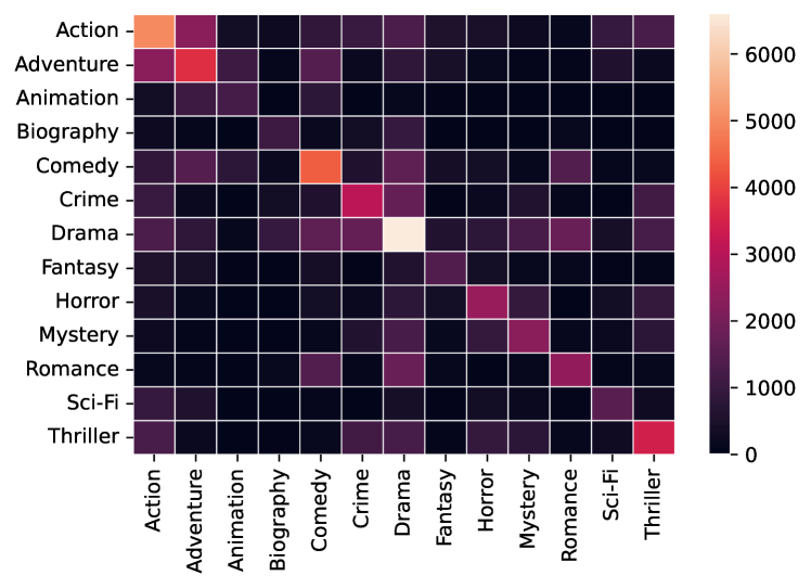
Figure A.1: Co-occurrence matrix for movie poster genres.

Appendix B Dataset Challenges

As mentioned in section I, the information contained within the posters introduces additional complexities when it comes to identifying the movie genre, and we briefly outline these challenges as follows.

(a) Background: The background of movie posters serves a significant purpose in establishing a sense of atmosphere or setting, piques curiosity, and helps individuals to make informed decisions about whether the movie aligns with their interests and preferences. For example, horror movie posters (Fig. C.1.v, xviii) often utilize specific background elements with dark shadows and eerie lighting to entice the viewers with a chilling, suspenseful, and frightening mood. Based on the information available on the poster background, we can further categorize it as below:

• Less information: Sometimes, a poster background may contain little to no information, which brings challenges to automated genre identification (Fig.s C.1.i-iv).

• Moderate & adequate information: Often, the background has sufficient visual characteristics to convey its genre (Fig.s C.1.v-vi).

• Complex background: In some cases, the background of a poster becomes complex due to having enormous and/or composite visual effects/elements (Fig.s C.1.vii-viiii).

(b) Foreground: The foreground in a poster plays a crucial role in capturing the viewer’s attention and creating visual interest. By strategically placing dynamic foreground elements, such as the main characters or key plot elements, the poster can effectively convey the theme or atmosphere of the movie. In the case of a romantic, comedy, featuring the two leads in a playful stance in the foreground may help in establishing the genre and the central focus of the film, which is the relationship between those characters (Fig. C.1.xii).

• Cast image: Often, the lead casts’ portrait, full/half body images cover the entire poster (Fig.s C.1.ix-xii), which makes our task challenging due to relying only upon visual elements without taking any aid from face recognition and object detection modules.

• Scene image: The scene images present in the entire poster sometimes brings challenges due to complex visual elements, visual clutter and lack of cohesive composition (Fig.s C.1.xiii-xiv).

• Cast in Scene: The hybridization of cast and scene images can also be observed, where the cast image may be fused with scene images (Fig.s C.1.xv-xvi).

(c) Inter variance: Often, different movie posters may have visual similarities while belonging to diverse genres. This can be done to challenge audience expectations, create intrigue, or highlight genre mashups. Such instances make the genre identification task quite difficult. For example, movie genre of Fig.s C.1.xviii poster is horror, but Fig. C.1.xvii does not, although visually quite similar; similarly, Fig.s C.1.xix and xx show non-identical genres, while sharing similar visual elements.

(d) Intra variance: Generally, a movie has multiple posters of various designs, where different designs may emphasize multiple aspects of the same movie to effectively market it to a diverse range of viewers, which brings additional challenges in identifying the genre. For example, Fig.s C.1.xxi and xxii are the posters from the same movie; however, they show variation in visual elements. Similarly, Fig.s C.1.xxiii and xxiv show intra-variation.

(e) Collage: Sometimes, a movie poster combines various instances of the abovementioned background and foreground information, and creates a collage made from tiny images. Such collage posters make genre identification challenging due to amalgamating a pool of information (Fig.s C.1.xxv-xxviii).

(f) Text $\leftrightarrow$ Image: In certain movie posters, some texts or titles are sometimes displayed as images rather than traditional typography (Fig.s C.1.xxix-xxxii). This artistic approach is often used to convey a specific theme or style associated with the movie. This brings additional challenges to our task, since we are not taking any aid from the text recognition module.

Appendix C Qualitative result: Heat map encoding

In Fig. C.2, we showcase the qualitative outcomes of ERDT through heat map encoding as mentioned in section IV-D. We have selected 20 sample posters, and present the corresponding ground-truth and ERDT-predicted heat map encodings using a gray color code.

i. (1, 2, 8)	ii. (7, 9, 10)	iii. (6, 7, 13)	iv. (10, 13, -)	v. (9, 10, 13)	vi. (5, 6, 7)	vii. (1, 12, -)	viii. (1, 2, 8)
less info				moderate/ adequate info		complex background
ix. (1, 2, 8)	x. (4, 7, -)	xi. (1, 10, 13)	xii. (11, 5, -)	xiii. (3, 1, 2)	xiv. (8, 9, 10)	xv. (1, 2, 5)	xvi. (2, 7, 12)
cast image				scene		cast + scene
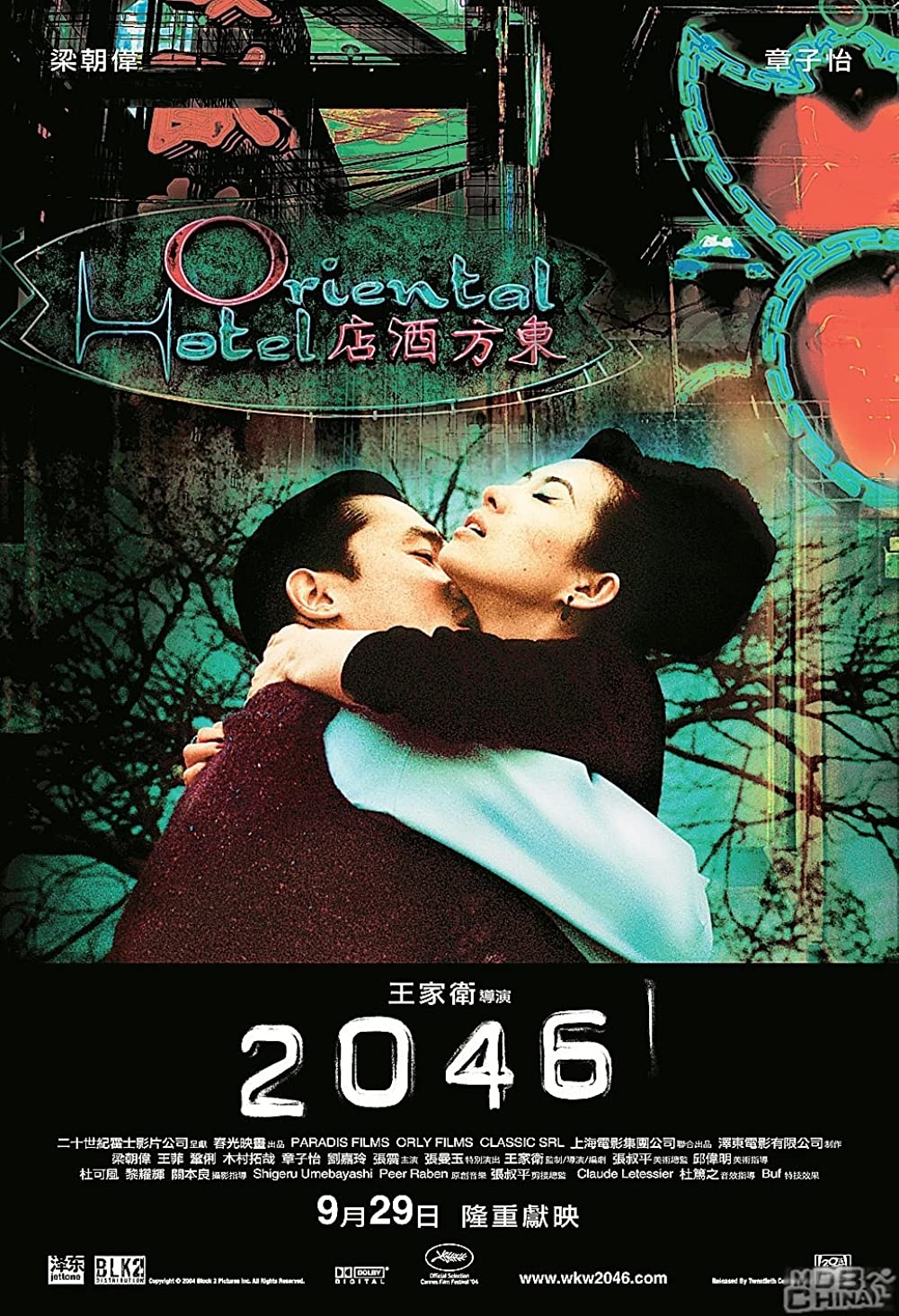
xvii. (10, 11, 7)	xviii. (9, 8, 7)	xix. (6, 7, 13)	xx. (5, 9, -)	xxi. (1, 2, 12)	xxii. (1, 2, 12)	xxiii. (7, 11, 12)	xxiv. (7, 11, 12)
inter-variation		inter-variation		intra-variation		intra-variation
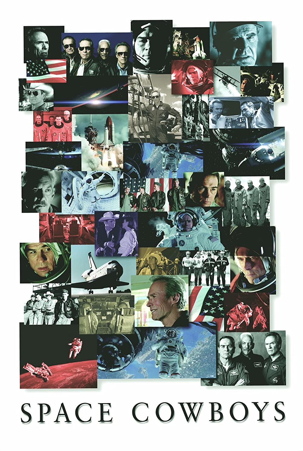
xxv. (6, 13, -)	xxvi. (1, 2, 13)	xxvii. (6, 10, 13)	xxviii. (7, 11, 12)	xxix. (3, 2, 5)	xxx. (1, 2, 8)	xxxi. (7, 12, -)	xxxii. (9, 10, -)
collage				text as image		image as text

Figure C.1: Examples of some challenging poster images with mentioned issues. Underneath each image, within the first bracket, the genre class numbers (refer to Table II) are also shown.

Ground-truth heat map of multi-hot encoding ERDT predicted confidence score heat map encoding Class ID 1 2 3 4 5 6 7 8 9 10 11 12 13 1 2 3 4 5 6 7 8 9 10 11 12 13

Figure C.2: Qualitative result: Ground-truth and ERDT-predicted heat map encodings in gray color code

References

- [1] J. A. Wi, S. Jang, and Y. Kim, “Poster-based multiple movie genre classification using inter-channel features,” IEEE Access, vol. 8, pp. 66 615–66 624, 2020.
- [2] P. Winoto et al., “The role of user mood in movie recommendations,” Expert Systems with Applications, vol. 37, no. 8, pp. 6086–6092, 2010.
- [3] M. Frey, Netflix recommends: algorithms, film choice, and the history of taste. Univ of California Press, 2021.
- [4] R. M. Lezama et al., “Trailers12k: Evaluating transfer learning for movie trailer genre classification,” arXiv:2210.07983, 2022.
- [5] A. Yadav and D. K. Vishwakarma, “A unified framework of deep networks for genre classification using movie trailer,” Applied Soft Computing, vol. 96, p. 106624, 2020.
- [6] Q. Hoang, “Predicting movie genres based on plot summaries,” arXiv:1801.04813, 2018.
- [7] J. Wehrmann et al., “Self-attention for synopsis-based multi-label movie genre classification,” in Int. FLAIRS Conf., 2018, pp. 236–241.
- [8] W.-T. Chu and H.-J. Guo, “Movie genre classification based on poster images with deep neural networks,” in Multimodal Understanding of Social, Affective and Subjective Attributes. ACM, 2017, p. 39–45.
- [9] F. Herrera et al., Multilabel Classification: Problem Analysis, Metrics and Techniques. Springer, 2016.
- [10] J. M. Johnson and T. M. Khoshgoftaar, “Survey on deep learning with class imbalance,” Journal of Big Data, vol. 6, pp. 1–54, 2019.
- [11] A. Dosovitskiy et al., “An image is worth 16x16 words: Transformers for image recognition at scale,” in ICLR, arXiv:2010.11929, 2021.
- [12] E. B.-Baruch et al., “Asymmetric loss for multi-label classification,” in CVPR, 2021, pp. 82–91.
- [13] G. S. Simões et al., “Movie genre classification with convolutional neural networks,” IJCNN, pp. 259–266, 2016.
- [14] X. Yuan et al., “Automatic Video Genre Categorization using Hierarchical SVM,” in ICIP, 2006, pp. 2905–2908.
- [15] S. Kar et al., “Folksonomication: Predicting tags for movies from plot synopses using emotion flow encoded neural network,” in ICCL, 2018, pp. 2879–2891.
- [16] P. J. Gorinski and M. Lapata, “What’s this movie about? a joint neural network architecture for movie content analysis,” in NAACL: Human Language Technologies, vol. 1. ACL, 2018, pp. 1770–1781.
- [17] I. R. Bribiesca et al., “Multimodal weighted fusion of transformers for movie genre classification,” in Workshop on MAI, 2021, pp. 1–5.
- [18] P. C. Bonilla et al., “Moviescope: Large-scale analysis of movies using multiple modalities,” arXiv:1908.03180, 2019.
- [19] H. Zhou et al., “Movie genre classification via scene categorization,” in ACM Multimedia, 2010, pp. 747–750.
- [20] J. Wehrmann and R. C. Barros, “Movie genre classification: A multi-label approach based on convolutions through time,” Applied Soft Computing, vol. 61, pp. 973–982, 2017.
- [21] M. Pobar et al., “Multi-label poster classification into genres using different problem transformation methods,” in CAIP, 2017, pp. 367–378.
- [22] N. Gozuacik et al., “Turkish movie genre classification from poster images using convolutional neural networks,” in ELECO, 2019, pp. 930–934.
- [23] A. M. Ertugrul et al., “Movie genre classification from plot summaries using bidirectional LSTM,” in ICSC. IEEE, 2018, pp. 248–251.
- [24] V. Battu et al., “Predicting the genre and rating of a movie based on its synopsis,” in PACLIC, 1–3 2018.
- [25] R. B. Mangolin et al., “A multimodal approach for multi-label movie genre classification,” Multimedia Tools and Applications, vol. 81, no. 14, pp. 19 071–19 096, 2022.
- [26] J. Arevalo et al., “Gated multimodal units for information fusion,” ICLR: Workshop arXiv:1702.01992, 2017.
- [27] Z. Rasheed and M. Shah, “Movie genre classification by exploiting audio-visual features of previews,” in ICPR, 2002, pp. 2: 1086–1089.
- [28] D. Brezeale and D. J. Cook, “Using closed captions and visual features to classify movies by genre,” in MDM/KDD, 2006, pp. 1–5.
- [29] K. Han et al., “A survey on vision transformer,” IEEE Trans. on PAMI, vol. 45, no. 1, pp. 87–110, 2023.
- [30] K. He, X. Zhang, S. Ren, and J. Sun, “Identity mappings in deep residual networks,” in ECCV, 2016, pp. 630–645.
- [31] M. Z. Alom et al., “The history began from AlexNet: A comprehensive survey on deep learning approaches,” arXiv:1803.01164, 2018.
- [32] A. Vaswani et al., “Attention is all you need,” Advances in neural information processing systems, vol. 30, 2017.
- [33] A. Zhang, Z. C. Lipton, M. Li, and A. J. Smola, “Dive into deep learning,” arXiv:2106.11342, 2021.
- [34] J. L. Ba et al., “Layer normalization,” arXiv:1607.06450, 2016.
- [35] D. P. Kingma and J. Ba, “Adam: A method for stochastic optimization,” arXiv:1412.6980, 2014.
- [36] L. Rokach, “Ensemble-based Classifiers,” Artificial intelligence review, vol. 33, no. 1, pp. 1–39, 2010.
- [37] L. Zahedi et al., “Search algorithms for automated hyper-parameter tuning,” in ICDATA, arXiv:2104.14677, 2021, pp. 1–10.
- [38] M.-L. Zhang and Z.-H. Zhou, “A review on multi-label learning algorithms,” IEEE Trans. on KDE, vol. 26, no. 8, pp. 1819–1837, 2013.
- [39] G. Huang et al., “Densely connected convolutional networks,” in CVPR, 2017, pp. 2261–2269.
- [40] M. Tan and Q. Le, “Efficientnet: Rethinking model scaling for convolutional neural networks,” in ICML, 2019, pp. 6105–6114.
- [41] C. Szegedy et al., “Rethinking the inception architecture for computer vision,” in CVPR, 2016, pp. 2818–2826.