Reconstructing Lattice Vibrations of Crystals with Electron Ptychography

Abstract

While capable of imaging the atoms constituting thin slabs of material, the achievable resolution of conventional electron imaging techniques in a transmission electron microscope (TEM) is very sensitive to the partial spatial coherence of the electron source, lens aberrations and mechanical instabilities of the microscope. The desire to break free from the limitations of the apparatus spurred the popularity of ptychography, a computational phase retrieval technique that, to some extent, can compensate for the imperfections of the equipment. Recently it was shown that ptychography is capable of resolving specimen features as fine as the blurring due to the vibrations of atoms, a limit defined not by the microscope, but by the investigated sample itself. Here we report on the successful application of a mixed-object formalism in the ptychographic reconstruction that enables the resolution of fluctuations in atomic positions within real space. We show a reconstruction of a symmetric $\Sigma$9 grain boundary in silicon from realistically (molecular dynamics) simulated data. By reconstructing the object as an ensemble of 10 different states we were able to observe movements of atoms in the range of 0.1-0.2 Å in agreement with the expectation. This is a significant step forward in the field of electron ptychography, as it enables the study of dynamic systems with unprecedented precision and overcomes the resolution limit so far considered to be imposed by the thermal motion of the atoms.

1 Introduction

Phase retrieval is an important technique for many types of scattering experiments. One of the most developed and effective approaches for addressing this task is called ptychography [1, 2, 3, 4, 5, 6, 7]. Numerous quite different variations of this technique exist, e.g. Fourier and near-field ptychography [8, 9], and a variety of reconstruction schemes for them. The ”classical” far-field ptychography recovers a complex transmission function of a specimen from a set of transmitted intensities collected while illuminating overlapping areas of its surface with a convergent beam.

Historically speaking, the interest in ptychography has fluctuated between two research areas: electron- and photon imaging. The essential theoretical ideas were formulated for electrons by Walter Hoppe and coauthors [2, 3, 4, 5]. While the most acknowledged experimental proof of principle was also done with electrons by Peter Nellist et alia [10], a compelling historical twist is that a few years before this publication, Stuart Friedman, who was as well as Peter Nellist a student of John Rodenburg, built and conducted a ptychographic experiment with laser [11], reinforcing the motivation to engage in such research with electrons. At the end of 1990’s the electron microscopes, detectors and computers were not well suited for the time consuming acquisitions and processing of large data-sets, performing electron ptychography on a daily basis was not possible, therefore the development of the method continued in the field of photon imaging and the first revolutionary applications of the technique were done with x-rays (e.g. [12]). The modern advancements in both hardware and software have completely reversed the relationship between the two research fields: the concepts initially formulated for (short wavelength) photons help to achieve record-breaking resolutions with electrons. Good examples are recently developed iterative ptychographic algorithms, e.g. the ones based on maximum-likelihood [13, 14] and mixed-probe formalism [15]. These two concepts introduced for photons allowed [6] to reach the limits set by lattice vibrations with an electron microscope, causing the resolution to be now be limited by the blurring of the projection of an atom by its thermodynamically defined motion about its equilibrium position.

One promising technique that extends conventional ptychography and allows overcoming this seemingly insurmountable limit is a mixed object formalism. This technique, closely related to a ”frozen phonon” formalism [6], was first described in the context of ptychography by Thibault and Menzel [15]. Previously there were attempts to apply this technique in expeiments with laser [7] and x-rays [16], however the applicability of the method to electron microscopy data at deep sub-Ångstrom resolution was not yet studied. Here, we report on the first successful application of the mixed-object formalism to a realistically simulated 4D-STEM dataset [1] of a symmetric $\Sigma$9 grain boundary in silicon [17, 18]. By reconstructing multiple states instead of one pure transmission function, we obtained a pseudo-temporal resolution and were able to observe lattice vibrations. It should be noted here that this process does not involve reducing the transmission function to a set of atom coordinates, even though, with a sufficiently high signal-to-noise ratio in the data, atom positions can be extracted from peaks in the transmission function. Below, we describe the underlying concepts and discuss the behaviour of the algorithm.

2 Theory

In far-field electron ptychography the input is a four dimensional scanning transmission electron microscopy (4D-STEM) dataset [1] containing diffraction patterns in terms of two real-space coordinates $\rho_{p,x}$, $\rho_{p,y}$ describing the beam position on the specimen’s surface and two reciprocal coordinates $k_{f,x}$ and $k_{f,y}$ indexing the pixels of the detector.

Strictly speaking, an iterative ptychographic algorithm fits a forward model that, for a given scanning position, maps an illumination wavefront to a measured diffraction pattern. This model includes a transmission function of the investigated sample and, as we will show further, can be formulated in various complexity levels. Recovering the initially unknown transmission function is the main goal of any ptychographic algorithm, as its amplitude characterises absorption and its phase is directly proportional to the specimen’s electrostatic potential. During the reconstruction one can additionally refine the probe [19, 20, 21], scan positions [20, 21, 22] or a mis-tilt angle between the optical axis of the microscope and the zone axis of the studied crystal [23]. Figure 1 shows various complexity levels in modelling the diffraction patterns. Developing the mixed-object formalism requires stepping through each stage of the diagram.

2.1 Two-dimensional Ptychography

When an electron beam passes through a sufficiently thin sample, it experiences only one scattering event. The three dimensional structure of an object can be simplified to two dimensions by integrating over the beam propagation direction. For a beam position $\rho_{p}$, the exit wave $P^{(exit)}(\rho_{p},\rho)$ can be calculated as a real space product of a two-dimensional wave function of the incident beam $P^{(in)}(\rho-\rho_{p})$ with a two-dimensional complex transmission function of a specimen $O(\rho)$:

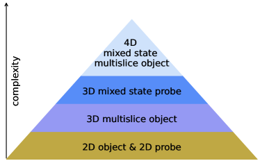
Figure 1: Diagram showing forward models with increasing complexity levels, i.e. an increasing number of operations to perform for a simulation of one diffraction pattern.

$$P^{(exit)}(\rho_{p},\rho)=P^{(in)}(\rho-\rho_{p})\cdot O(\rho).$$ (1)

After switching from real to reciprocal space one can compute the corresponding diffraction pattern:

$$I(\rho_{p},k_{f})=\left|\mathcal{F}\left\{P^{(exit)}(\rho_{p},\rho)\right\}\right|^{2}.$$ (2)

The reconstruction process is typically [20, 21, 13] organised as a gradient-descent minimisation of a metric, i.e. a loss function, describing the discrepancy between the measured intensities and the ones predicted by the forward model. This study employs an $l_{2}$ norm i.e. a summed squared error:

$$\mathcal{L}=\sum|I^{m}-I|^{2}$$ (3)

Due to the finite amount of available memory, the estimation of the loss and the subsequent gradient descent updates of the object and probe are computed either for individual scan positions or, alternatively, in a mini-batch fashion for a small number of positions. Until the loss becomes small enough, one has to iterate and apply the following update rules to the optimised parameters:

$$A_{n+1}=A_{n}-\alpha\cdot\frac{\partial\mathcal{L}}{\partial A_{n}^{*}}$$ (4)

here $A$ is an optimised unknown, such as object, probe, probe positions etc., $n$ indicates the iteration, $*$ denotes the conjugated Wirtinger derivative [24, 25, 14, 26] of the loss function with respect to $A$, and $\alpha$ is a real and positive scalar (update step).

2.2 Multi-slice formalism

Decreasing beam energy and increasing the thickness of a specimen make the effect of multiple scattering more pronounced. The authors of [6] showed that at some point the thin object approximation described in subsection 2.1 starts to fail. In this case the most efficient strategy is to ”divide and conquer”. Instead of using one two dimensional transmission function, one can split the propagation direction into multiple intervals and define a set of 2D transmission functions responsible for each particular sufficiently thin region. We can write

$$P^{(exit)}_{j}(\rho_{p},\rho)=P^{(in)}_{j}(\rho-\rho_{p})\cdot O_{j}(\rho),$$ (5)

where $j$ indicated a particular interval, i.e. slice. The propagation between the neighbouring slices $j$ and $j+1$ over the interval d is calculated via a convolution with a Fresnel propagator:

$$P^{(in)}_{j+1}(\rho)=\mathcal{F}^{-1}\left\{\mathcal{F}\left\{P^{(exit)}_{j}(\rho)\right\}\cdot\mathcal{P}_{Fr}\left(k\right)\right\}$$ (6)

$$\mathcal{P}_{Fr}\left(k\right)=exp\left[i\pi\lambda d|k|^{2}\right],$$ (7)

where $\lambda$ is a wavelength of the electron beam and the equation 7 defines the Fresnel propagator in reciprocal space. Typically one chooses the distance between the slices of approximately 1-3 nm (see e.g. [6, 27]). The $P^{(in)}_{j=0}(\rho-\rho_{p})$ is the incident illumination wavefront and for N slices the exit-wave $P^{(exit)}_{j=N}(\rho)$ is used to calculate a diffraction pattern as described in the equation 2.

2.3 Mixed-probe formalism

All previous derivations assumed a stationary illumination wavefront, however in a real experimental situation, it is not always appropriate to neglect the partial spatial coherence of the electron source and vibrations of the atoms. To account for partial spatial coherence, Thibault and Menzel [15] proposed to replace the pure probe state $P^{(in)}_{j=0}(\rho)$ with a statistical mixture of multiple probe states $P^{(in)}_{j=0,m}(\rho)$, where the first index $j=0$ remained from the multi-slice formalism and the second index m accounts for multiple modes. The total predicted diffraction pattern is calculated as an incoherent sum of the intensities corresponding to the individual probe modes. Let $I^{(1)}(P^{in}_{j=0}(\rho-\rho_{p}),O(\rho))$ denote the sequence of operations described in the subsection 2.2 applied to a single probe mode. In mixed-probe formalism, the intensity is modelled as

$$I_{total}=\sum_{m=0}^{N_{{probe\ modes}}}I^{(1)}(P^{in}_{j=0,m}(\rho-\rho_{p}),O(\rho)).$$ (8)

2.4 Mixed-object formalism

The mixed-object formalism is a natural extension of the mixed-probe formalism that accounts for a non-stationary object’s transmission function. Due to the lattice vibrations and the corresponding displacements of the atoms, two electrons hitting the specimen at exactly the same spatial position but at two different points in time interact with slightly different electrostatic potentials. To account for this effect, i.e. thermal diffuse scattering (TDS) [28], one can use multiple transmission functions and model a diffraction pattern as an incoherent sum of the intensities corresponding to the individual pure transmission functions.

$$I_{total}=\sum_{n=0}^{N_{{object\ modes}}}\sum_{m=0}^{N_{{probe\ modes}}}I^{(1)}(P^{in}_{j=0,m}(\rho-\rho_{p}),O_{n}(\rho))$$ (9)

Thus, in the most complex scenario one has to deal with a three dimensional illumination wavefront (2 lateral dimensions plus one dimension for multiple modes), a four dimensional object (2 lateral dimensions and two dimensions one each for multiple slices and multiple modes) and perform $N_{{object\ modes}}\times N_{{probe\ modes}}$ forward multi-slice propagations to model one diffraction pattern. Given the fact that gradient descent ptychographic reconstruction requires repeating this type of calculation hundreds or thousands of times in order to achieve convergence, the whole computation can be called ”computationally expensive”. For a long time, one could use such formalism only for simulation of STEM images [28, 29], where the procedure does not have to be repeated. Nonetheless, modern GPUs untie the hands of researchers and now allow more complex calculations.

3 Simulation with thermal diffuse scattering

We used 30 atomic configurations from a molecular dynamics (MD) simulation of a 7 Å thick (four atomic layers) symmetric $\Sigma$9 grain boundary in silicon [17, 18] to simulate a 4D-STEM dataset using the python package abTEM [30]. The accelerating voltage, convergence semi-angle, and scan-step were 60 kV, 30 mrad, and 0.3 Å, respectively, and an infinite dose was assumed. By summing the neighbouring diffraction patterns with gaussian-weighting the effect of partial spatial coherence with an effective source size of 0.2 Å was reproduced. We performed three different multi-slice ptychographic reconstructions from the simulated dataset, the first with pure object and pure probe, the second one with pure object and 5 states of mixed-probe, and the last one with 10 states of mixed-object and 5 states of mixed-probe, as described in sections 2.2, 2.3 and 2.4, respectively. In all reconstructions presented further, we used 2 slices and a spacing of 3 Å. Calibration runs showed that using more slices and covering larger intervals along the beam propagation direction was not necessary as the extra slices contained no information about the sample and were empty upon convergence of the reconstruction.

An initial guess for the illumination was based on the inverse Fourier transform of the mean diffraction pattern. After a series of calibration runs, more optimal probes for each of the three reconstructions were fit and the runs re-started. The initial guess for the object was based on uniform prior. For a mixed-object reconstruction, the following is a crucial part: if the initial guess for each state is the same, the updates applied to them (see eq. 4) become identical. As a result, it would not be possible to reconstruct the movement of the atomic columns. Important to mention is the fact that we used all diffraction patterns at once to form one update direction, otherwise the potential was unevenly distributed across the states and the reconstruction appeared nonphysical. A similar problem was observed in the experiment with photons [7]. Figure 11 showing a corresponding failed reconstruction can be found in the appendix. In Figure 2 we demonstrate an average slice (and state) for the three reconstructions. Figure 3 shows both Fourier transform (FT) and power spectra of the three reconstructions. Note that in both Figures, the effect of time-averaging is damping the unwanted noise between the atoms and makes the higher spatial frequencies more pronounced.

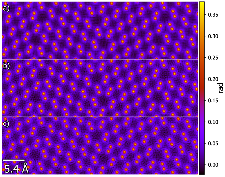
Figure 2: Phase of a mean slice (and state) for a) mixed-object and mixed-probe reconstruction b) pure-object and mixed-probe reconstruction c) pure-object and pure-probe reconstruction. The colorbar is in radians. The image a) can be considered as a time average of the potential, while the other two reconstructions represent the most suitable static potential for data obtained with time-varying atomic positions. One can see that the mixed-object reconstruction is less affected by noise between the atomic columns.

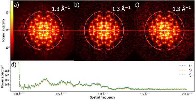
Figure 3: Average over slices and states of a squared absolute value of the Fourier transformed reconstructed transmission functions with a) mixed-object and mixed-probe b) pure object and mixed-probe and c) pure object and pure probe. d) Power spectra (azimuthal averages) of a)-c). The white circles in a)-c) indicate the information limit of 1.3 Å^-1 reached by all three reconstructions. The mixed-object reconstruction a) appears to outperform the other two cases, as it contains visually recognisable frequencies higher than 1.6 Å^-1, while b) and c) are more affected by noise. Note that in all three cases we limited the bandwidth to half of the highest spatial frequency to completely eliminate the possibility of aliasing.

In contrast to previous research, e.g. [6], both Figures 2 and 3 show that in our particular case one does not benefit from the mixed-probe formalism [15]. The amount of partial spatial coherence introduced into the data in the simulation was not severe enough to benefit from this approach, while the algorithm was struggling with unnecessarily many probe states. This also affected the convergence of the algorithm, in Figure 4 we show the loss function that was minimized during the reconstruction as a function of iteration. Note that the plotted loss is summed over all 233$\times$233 pixels of the detector and all 8134 scan positions. Thus, an error of order $10^{-3}$ is a rather small quantity (the mean value of the whole 4D-STEM dataset is 7.06e-6). Still, the mixed-probe and pure-object reconstruction provides a worse match between measurement and reconstruction than the other two cases. Potentially that could be caused by the fact that the optimizer applied in this ptychographic reconstruction algorithm can never drive the extra probe modes to an absolute zero and the residual small intensity produces a higher loss value.

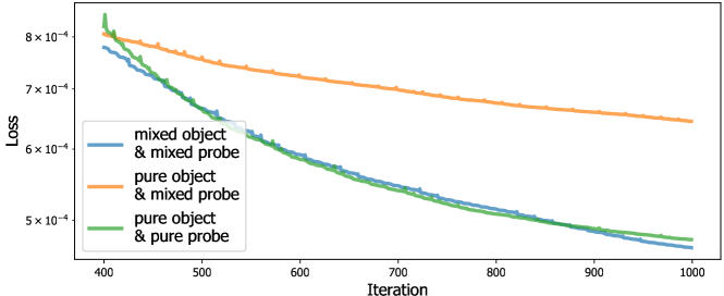
Figure 4: Loss, i.e. a summed squared error between the measured and predicted diffraction patterns, as a function of iteration. At the beginning, the pure object and pure probe reconstruction (green line) appears to outperform the other two cases, while the mixed-object reconstruction (blue line) starts to produce a slightly better loss after approximately 950 cycles across all scan positions. Generally, this trend emphasizes the fact that mixed-object reconstruction requires a lot of computation time to bring any benefits. The pure-object and mixed-probe reconstruction (orange line) due to over-specified probe shows a worse convergence and produces a higher loss.

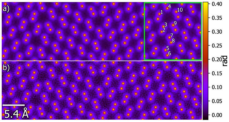
Figure 5: Phase of a mean slice (and state) for a) mixed-object and pure-probe reconstruction b) pure-object and pure-probe reconstruction. The colorbar is in radians. Both images are produced after 2000 iterations i.e. full cycles through all 8134 scan positions contained in the 4D-STEM dataset. The image a) can be considered as a time average of a potential, while b) represents the most suitable static potential for data obtained with time-varying atomic positions. As in Figure 2 one can see that the mixed-object reconstruction is less affected by noise between the atomic columns. The states of the reconstruction a) in the region indicated by the lime-colored box are individually shown in Figure 8. The position fluctuations of atomic columns marked with numbers from 1 to 9 are further analysed in Figure 9

As the mixed-object reconstruction presented in panel a) of Figure 2 was also done with a mixed-probe, we supposed that combining mixed-object reconstruction with pure-probe might be more beneficial in case of this particular dataset. To test this hypothesis we took only the first probe mode of the mixed-object reconstruction and started once again from random noise. A competing pure probe and pure object reconstruction was initialized using the probe reconstructed from the previous pure-probe and pure-object run, the object was also initialised using random noise. The recovered phases, Fourier transforms and loss functions are compared in Figures 5, 6 and 7, respectively.

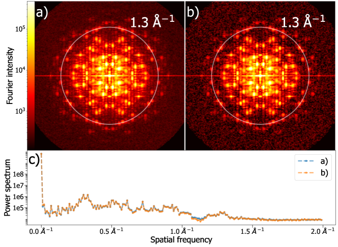
Figure 6: Average over slices and states of a squared absolute value of the Fourier transformed reconstructed transmission functions with a) mixed-object and pure probe and b) pure object and pure probe. c) Power spectra (azimuthal averages) of a) and b). The white circles indicate the information limit of 1.3 Å^-1 reached by the two competing reconstructions, as well as by three previous runs presented in Figures 2 and 3.

Figure 7: Loss, i.e. a summed squared error between the measured and predicted diffraction patterns, as a function of iteration. Combined with a pure-probe, mixed-object (blue line) outperforms the pure-object (orange line) and leads to a smoother reduction of the loss. The orange line is not decaying monotonically, indicating that the pure-object reconstruction is possibly oscillating about a local minimum.

Both Figures 5 and 6 support the previous observations: incoherent averaging over the states reduces noise in both, the reconstructed phase, and the Fourier transform of the transmission function. Note that this effect is not visible in the power spectrum, where azimuthal averaging erases the advantages of mixed-object reconstruction by not differentiating between structural information and noise.

For a pure-probe, the mixed-object reconstruction leads to a notably better loss values than the reconstruction of a pure-object. The error of the pure-object reconstruction represented by the orange line in Figure 7 is not decaying monotonically, potentially indicating that the reconstruction oscillates about a local minimum. This behaviour was not observed in case of the mixed-object reconstruction (blue line in the same Figure), it is reduced smoothly and converges towards a smaller error than the mixed-object and mixed-probe reconstruction from the Figure 4. This more smooth behaviour is likely due to the much larger parameter space available to the optimization algorithm.

In Figure 8 we show the mean slices of the object states in a region marked by the lime-colored box in Figure 5. For each atomic column in each of ten states we calculated the position by computing the center of mass of the reconstructed phase within a 5 pixel radius around the corresponding atomic column, i.e. summing the product of the distance of each pixel within the 5-pixel radius from the time-averaged position of the atomic column and the reconstructed phase as a weighting factor and then dividing this sum by the sum of the unweighted distances of each pixel from the atomic column. Since the true positions of the atomic columns used for the simulation of the 4D-STEM dataset are known, we were able to compare the two sets of xy-coordinates with each other. The comparison is presented in Figure 9.

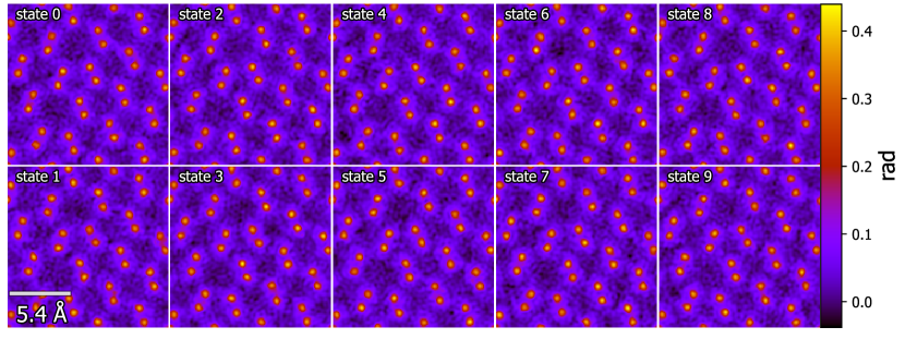
Figure 8: Individual states of the mixed-object and pure-probe reconstruction in a sub-region indicated by the lime box in Figure 5. One can see that the states are affected by noise in a same way as for the pure-object reconstructions. The changes of the atomic positions are not very apparent in this representation of the results, however one should notice the intensity-fluctuations and changes of atomic shapes in the phase which have an effect on the center of mass of these peaks.

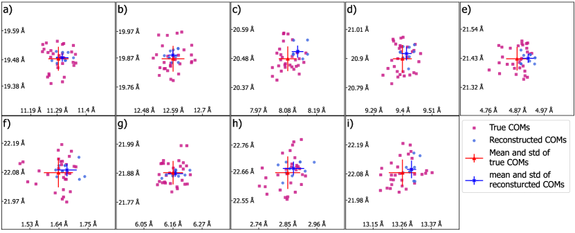
Figure 9: a)-i) Scatter charts of the x and y positions of the center of mass (COM) for 9 different atomic columns that are marked with numbers 1-9 in panel a) of Figure 5. Blue points correspond to the COMs from the reconstructed data and the magenta points are the original positions of the atoms used for the 4D-STEM simulation including TDS. The dark blue and red error bars represent mean values and standard deviations of the true and reconstructed data-sets, respectively.

4 Simulation without thermal diffuse scattering

Figure 9 shows a possible set of reconstructed positions of the atomic columns from the data simulated by including the thermal motion of the atoms. In order to test whether the reconstruction algorithm can also detect the absence of vibrations in data generated from a stationary electrostatic potential, simulated without TDS, we simulated [30] an additional 4D-STEM data-set [1] from a single snapshot of the MD-simulation of the same $\Sigma$9 grain boundary in silicon [17, 18] with the same beam energy (60 keV), convergence semi-angle (30 mrad) and scan step size (0.3 Å). Even though the Figures 2, 3 and 4 point to the fact that the amount of partial spatial coherence introduced into the previous data-set was negligible, we did not add it to the new data-set in order to simulate a perfectly stationary experimental condition. Similar to previous reconstructions, we did a series of calibration runs to fit an optimal probe and restarted the reconstruction beginning with uniform prior (see e.g. [21]) for all 10 states of the mixed-object. Results of the reconstruction after 4000 iterations are shown in Figure 10.

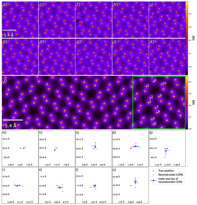
Figure 10: Mixed-object reconstruction from the data simulated with stationary atomic positions and without partial spatial coherence of the electron source. Panels a)-k) show mean slices of the 10 states in a sub-region indicated by the lime-colored box in panel l) presenting the full phase averaged over 10 states and 2 slices. Scatter charts m)-u) the x and y positions of the center of mass (COM) for the atomic columns marked with numbers 1-9 in panel l). Note that the standard deviations marked with blue error bars are much smaller than in Figure 9. In panels m) and n) the 10 extracted positions converge almost to one point.

5 Discussion

The experimental discovery of thermal streaks in electron diffraction patterns [31, 32] is as old as the ideas of ptychography [2, 3, 4, 5]. The impact of lattice vibrations on the electron diffraction was heavily investigated both experimentally and theoretically during the last century (e.g. [33]) and is still a hot research topic nowadays (e.g. [34]). From a perspective of computational physics, standing between the theory and experiment, the main research paper came out at the beginning of the new millennium. It was demonstrated [29] that faint structure in the diffuse Kikuchi diffraction intensity between the Bragg spots of electron diffraction patterns allow one to distinguish between different kinds of lattice vibrations. Uncorrelated atomic displacements, i.e. vibrations according to the Einstein model, result in slightly different diffraction patterns than displacements generated from a detailed phonon dispersion curve. Since that time it was somewhat intuitively clear that there must be a way to invert this dependence and draw conclusions about correlations in the vibrations of the atoms by looking at the diffraction patterns. Albeit, a suitable initial path for reconstructing the motion of the atoms and the necessary computational power were missing. The presented analysis of the reconstruction validates the possibility of such an inversion. Moreover, we want to emphasize the fact, that modern GPUs allow for a significantly accelerated reconstruction process. For our in-house-written code utilizing the Python library CuPy [35], 2000 iterations of the pure-object and pure-probe reconstructions presented in panel b) of Figure 5 took 28.5 hours to run on a single NVIDIA TESLA V100 GPU [36]. 2000 iterations of the pure-probe and mixed-object reconstruction with 10 transmission function states presented in Figure 5a and Figure 8 required only twice as much time, 45.1 hours. It is noteworthy that the whole process can be trivially parallelized and accelerated by spreading multiple scan-positions, beam-states, or object-states over multiple GPUs.

The standard deviations of the positions of the reconstructed atomic columns presented in Figure 9 are slightly smaller than the true values used for the simulation of the 4D-STEM data set. Nevertheless, the spreads of true and reconstructed atomic column COMs appear to be similar. This proof of the possibility of reconstructing lattice vibrations is also supported by the results of the mixed-object reconstruction from the data simulated with stationary atomic positions (no TDS) presented in Figure 10. It shows that the ptychographic algorithm can partially recognize the absence of vibrations. The word ”partially” is referring to the fact that the standard deviations of the reconstructed atomic column COMs in Figure 10 are not truly zero, but still, noticeably smaller than those shown in Figure 9. The trend of the reconstruction implies that after more iterations the standard deviations might get even smaller, e.g. like in panels m) or n) of Figure 10, but there is no guarantee that the algorithm will not converge to a local minimum.

As the presented tests of the mixed-probe formalism have shown, adding more degrees of freedom to the reconstruction than required can spoil the convergence. On one hand, this might be caused by an orthogonality-restriction we put on the probe states. The Gram-Schmidt algorithm was applied to the modes after each iteration. Thus, there was no possibly for the probe modes to become similar and the small amount of intensity contained in the extra modes lifted the loss up for both pure- (see Figure 4) and mixed-objects (see Figure 7). On the other hand, looking at it from a reciprocity perspective [37] finite electron source width in STEM is equivalent to a miniscule detector pixel in TEM, way less than the ”resolution”. Thus, the amount of the partial spatial coherence introduced is insufficient to fully utilize the power of the mixed-probe formalism. Since this work is focused on the mixed-object reconstruction, exploring from what point the partial spatial coherence introduced into the data by summing the neighbouring diffraction patterns with Gaussian weights really requires additional probe states and how to properly enforce their orthogonality is left for future research.

Both Figures 4 and 7 show that the mixed-object formalism produces a better fit to the data simulated with account of thermal diffuse scattering. Moreover, an incoherent time-averaging can serve as a noise reduction tool. For our algorithm based on gradient-descent minimization, Figures 3 and 6 show that the mixed-object formalism provides a cleaner Fourier transform of the reconstructed phase. The corresponding reduction in noise can also be observed in the real space representations of the reconstructed phase. While the individual states of the mixed-object presented in Figures 8 appear to be as noisy as the pure-object reconstructions presented in panels b) and c) of Figure 2 and panel b) of Figure 5, the time-averaged phases from panels a) of Figures 2 and 5 have less signal between the atoms. Figure 10 shows that even for the data-set simulated without TDS, the reconstructed phase averaged over 10 states has less noise between the atoms than the individual states presented in the same Figure. Thus, the mixed-object formalism might be employed to increase signal-to-noise ratio regardless of whether the atomic vibrations are contributing to the data or not.

In the reconstruction of actual experimental data one must emphasize that even though ptychography can compensate some experimental imperfections, it is unlikely capable of compensating them completely. It is also important to consider the electron dose since ptychographic reconstruction with high spatial resolution requires a lot of input information in order to provide a decent output. For the recently published reconstructions showing record-breaking resolution [6, 23, 38], for example, an electron dose not smaller than $1e6$ $e^{-}/\AA^{2}$ was applied. The reconstructions from simulated data presented in the current work were obtained at an infinite dose. In the near future we intend to perform reconstructions from real experimental data to test the limitations of the algorithm.

An unexpected outcome of this study is the fact that the success of the reconstruction is based on the number of diffraction patterns contributing to one gradient. The larger the area of the sample covered during one update, the higher the probability that the reconstruction will converge towards a physically reasonable result. In Figure 11 in the appendix we show results of one failed run where instead of all 8134 diffraction patterns, we used only 166 to form a mini-batch [21, 13]. In this case, one can barely recognize the atomic columns in the individual states, while the time average presented in panel l) of Figure 11 is quite similar to the one presented in Figure 2a. This problem might be solved by imposing various constraints. Peng Li and coauthors during a previously mentioned mixed-object experiment with photons [7] were able to increase the quality of the results reconstructed using the ePIE algorithm [19] by prohibiting absorption. Nevertheless, since ePIE is designed to treat one scan position after another, one might need to construct stronger restrictions to fully counteract the recovery of non-physical states if one wants to use this algorithm.

Our results open new possibilities for investigations of thermostated samples as one can observe the difference in dynamics of the same system under different external conditions at the atomic level. This might be useful for the studies of general mechanical properties or, for example, the analysis of defects in crystals.

Appendix A Update direction formation

During the tests of the reconstruction parameters we noticed that the algorithm behaves quite differently depending on one setting-the number of diffraction patterns (or scan positions) that are used to form one update direction. Visually appealing results, e.g. the one presented in Figure 8, were only achievable in cases where all diffraction patterns at once contributed to the gradient of the loss function. In all other scenarios, phase was distributed unevenly across the slices. The panels a)-k) of Figure 11 demonstrate this problem. In this case only 166 of 8134 randomly selected diffraction patterns contributed to one update batch [21]. The sum of states (time-average) shown in panel l) of Figure 8 is identical to the one shown in Figure 2.

Note that not all iterative ptychographic algorithms are capable to use all diffraction at the same time to form one update batch. Some of them, e.g. ePIE [19, 7] are constructed to treat one scan position after another. Based on our observations, one has to construct supporting constraints if one wants to use such algorithms with mixed-object formalism.

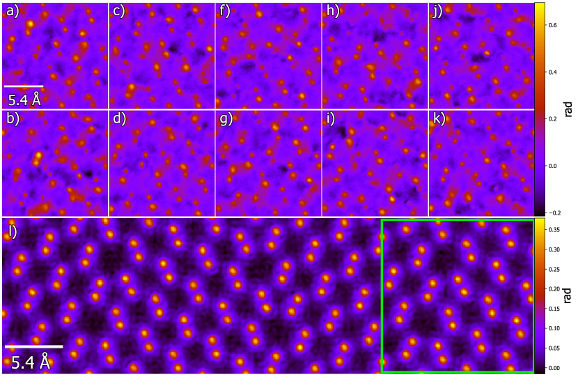
Figure 11: Failed mixed-object reconstruction where the update was formed not by all 8134 diffraction patterns. Panels a)-k) show the 10 states of the phase in a region indicated by the lime-colored box in panel l). The panel l) shows sum of the 10 states that can be treated as a time average of the electrostatic potential.

References

- [1] Colin Ophus “Four-Dimensional Scanning Transmission Electron Microscopy (4D-STEM): From Scanning Nanodiffraction to Ptychography and Beyond” In Microscopy and Microanalysis 25, 2019, pp. 1–20 DOI: 10.1017/S1431927619000497
- [2] Walter Hoppe “Beugung im inhomogenen primärstrahlwellenfeld. i. prinzip einer phasenmessung von elektronenbeungungsinterferenzen” In Acta Crystallographica Section A: Crystal Physics, Diffraction, Theoretical and General Crystallography 25.4 International Union of Crystallography, 1969, pp. 495–501
- [3] Walter Hoppe and G. Strube “Beugung in inhomogenen primärstrahlenwellenfeld. II. lichtoptische analogieversuche zur phasenmessung von gitterinterferenzen.” In Acta crystallographica. Section A, Foundations of crystallography 25.4, 1969, pp. 501–508
- [4] Walter Hoppe “Beugung im inhomogenen Primärstrahlwellenfeld. III. Amplituden-und Phasenbestimmung bei unperiodischen Objekten” In Acta Crystallographica Section A: Crystal Physics, Diffraction, Theoretical and General Crystallography 25.4 International Union of Crystallography, 1969, pp. 508–514
- [5] Reiner Hegerl and Walter Hoppe “Dynamische theorie der kristallstrukturanalyse durch elektronenbeugung im inhomogenen primärstrahlwellenfeld” In Berichte der Bunsengesellschaft für physikalische Chemie 74.11 Wiley Online Library, 1970, pp. 1148–1154
- [6] Zhen Chen et al. “Electron ptychography achieves atomic-resolution limits set by lattice vibrations”, 2021
- [7] Peng Li et al. “Breaking ambiguities in mixed state ptychography” In Optics Express 24, 2016, pp. 9038 DOI: 10.1364/OE.24.009038
- [8] Guoan Zheng et al. “Concept, implementations and applications of Fourier ptychography”, 2021, pp. 207–223 DOI: 10.1038/s42254-021-00280-y
- [9] Shengbo You et al. “Magnetic Phase Imaging using Lorentz Near-field Electron Ptychography”, 2023
- [10] P.. Nellist, B.. McCallum and J.. Rodenburg “Resolution beyond the ’information limit’ in transmission electron microscopy” In Nature 374.6523, 1995, pp. 630–632 DOI: 10.1038/374630a0
- [11] Stuart L Friedman and JM Rodenburg “Optical demonstration of a new principle of far-field microscopy” In Journal of Physics D: Applied Physics 25.2 IOP Publishing, 1992, pp. 147
- [12] John Rodenburg et al. “Hard-X-Ray Lensless Imaging of Extended Objects” In Physical review letters 98, 2007, pp. 034801 DOI: 10.1103/PhysRevLett.98.034801
- [13] Michal Kronenberg, Andreas Menzel and Manuel Guizar-Sicairos “Iterative least-squares solver for generalized maximum-likelihood ptychography” In Optics Express 26, 2018, pp. 3108 DOI: 10.1364/OE.26.003108
- [14] P. Thibault and Guizar-Sicairos M. “Maximum-likelihood refinement for coherent diffractive imaging” In New Journal of Physics 14(6):063004, doi: 10.1088/1367-2630/14/6/063004, 2012
- [15] Pierre Thibault and Andreas Menzel “Reconstructing state mixtures from diffraction measurements” In Nature 494, 2013, pp. 68–71 DOI: 10.1038/nature11806
- [16] Björn Enders “Development and application of decoherence models in ptychographic diffraction imaging”, 2016
- [17] Benedikt Haas et al. “Atomic-Resolution Mapping of Localized Phonon Modes at Grain Boundaries” In Nano letters 23, 2023 DOI: 10.1021/acs.nanolett.3c01089
- [18] Peter Rez, Tara Boland, Christian Elsässer and Arunima Singh “Localized Phonon Densities of States at Grain Boundaries in Silicon” In Microscopy and Microanalysis 28, 2022, pp. 1–8 DOI: 10.1017/S143192762200040X
- [19] A.M. Maiden and J.M. Rodenburg “An improved ptychographical phase retrieval algorithm for diffractive imaging” In Ultramicroscopy 109(10):1256-62, doi: 10.1016/j.ultramic.2009.05.012, 2009
- [20] Marcel Schloz et al. “Overcoming information reduced data and experimentally uncertain parameters in ptychography with regularized optimization” In OpticsExpress 28.19, 2020, pp. 28306–28323
- [21] Ming Du et al. “Adorym: A multi-platform generic X-ray image reconstruction framework based on automatic differentiation” In Optics express 29.7 Optica Publishing Group, 2021, pp. 10000–10035
- [22] Andrew Maiden et al. “An annealing algorithm to correct positioning errors in ptychography” In Ultramicroscopy 120, 2012, pp. 64–72 DOI: 10.1016/j.ultramic.2012.06.001
- [23] Sha Haozhi, Cui Jizhe and Rong Yu “Deep sub-angstrom resolution imaging by electron ptychography with misorientation correction” In Science Advances 8, 2022 DOI: 10.1126/sciadv.abn2275
- [24] W. Wirtinger “Zur formalen Theorie der Funktionen von mehr komplexen Veränderlichen” In Math. Ann. 97, 1927, pp. 357–375 DOI: 10.1007/BF01447872
- [25] Reinhold Remmert and R.. Burckel “Theory of Complex Functions”, 1990 URL: https://api.semanticscholar.org/CorpusID:117813740
- [26] Adam Paszke et al. “PyTorch: An Imperative Style, High-Performance Deep Learning Library” In Advances in Neural Information Processing Systems 32 Curran Associates, Inc., 2019
- [27] Hamish Brown et al. “A Three-Dimensional Reconstruction Algorithm for Scanning Transmission Electron Microscopy Data from a Single Sample Orientation” In Microscopy and Microanalysis 28, 2022, pp. 1–9 DOI: 10.1017/S1431927622012090
- [28] P. R.. and J. Silcox “Thermal Vibrations in Convergent-Beam Electron Diffraction” In Acta Cryst. A 47, 1991, pp. 267–278
- [29] David Muller, Byard Edwards, Earl Kirkland and J. Silcox “Simulation of thermal diffuse scattering including a detailed phonon dispersion curve” In Ultramicroscopy 86, 2001, pp. 371–80 DOI: 10.1016/S0304-3991(00)00128-5
- [30] Jacob Madsen and Toma Susi “The abTEM code: transmission electron microscopy from first principles” In Open Research Europe 1, 2021, pp. 24 DOI: 10.12688/openreseurope.13015.1
- [31] G Honjo “Proc. Int. Conf. Mag. and Cryst. 1961, Kyoto, II” In J. Phys. Soc. Japan 17.B-II, 1962, pp. 277
- [32] Goro Honjo, Shiro Kodera and Norihisa Kitamura “Diffuse streak diffraction patterns from single crystals I. General discussion and aspects of electron diffraction diffuse streak patterns” In Journal of the Physical Society of Japan 19.3 The Physical Society of Japan, 1964, pp. 351–367
- [33] Jian-Min Zuo and Peter Rez “Observation of the structural phase transition in SrFio 3 by diffuse electron scattering” In Proceedings, annual meeting, Electron Microscopy Society of America 48, 1990, pp. 420–421 DOI: 10.1017/S0424820100175235
- [34] Tore Niermann “Scattering of fast electrons by lattice vibrations” In Phys. Rev. B 100 American Physical Society, 2019, pp. 144305 DOI: 10.1103/PhysRevB.100.144305
- [35] Ryosuke Okuta et al. “CuPy: A NumPy-Compatible Library for NVIDIA GPU Calculations” In Proceedings of Workshop on Machine Learning Systems (LearningSys) in The Thirty-first Annual Conference on Neural Information Processing Systems (NIPS), 2017 URL: http://learningsys.org/nips17/assets/papers/paper_16.pdf
- [36] “NVIDIA TESLA V100 GPU ARCHITECTURE”, 2017 URL: https://images.nvidia.com/content/volta-architecture/pdf/volta-architecture-whitepaper.pdf
- [37] H Rose and Christian Kisielowski “On the Reciprocity of TEM and STEM” In Microscopy and microanalysis : the official journal of Microscopy Society of America, Microbeam Analysis Society, Microscopical Society of Canada 11, 2005, pp. 2114–2115 DOI: 10.1017/S1431927605507761
- [38] Yi Jiang et al. “Electron ptychography of 2D materials to deep sub-ångström resolution” In Nature 559, 2018 DOI: 10.1038/s41586-018-0298-5