Data-driven models for predicting the outcome of autonomous wheel loader operations

Abstract

This paper presents a method using data-driven models for selecting actions and predicting the total performance of autonomous wheel loader operations over many loading cycles in a changing environment. The performance includes loaded mass, loading time, work. The data-driven models input the control parameters of a loading action and the heightmap of the initial pile state to output the inference of either the performance or the resulting pile state. By iteratively utilizing the resulting pile state as the initial pile state for consecutive predictions, the prediction method enables long-horizon forecasting. Deep neural networks were trained on data from over 10,000 random loading actions in gravel piles of different shapes using 3D multibody dynamics simulation. The models predict the performance and the resulting pile state with, on average, 95% accuracy in 1.2 ms, and 97% in 4.5 ms, respectively. The performance prediction was found to be even faster in exchange for accuracy by reducing the model size with the lower dimensional representation of the pile state using its slope and curvature. The feasibility of long-horizon predictions was confirmed with 40 sequential loading actions at a large pile. With the aid of a physics-based model, the pile state predictions kept sufficiently accurate for longer-horizon use.

1 Introduction

Recent advances in artificial intelligence suggest that computerized control of construction and mining equipment has the potential to surpass that of human operators. Fully or semi-autonomous wheel loaders, not relying on experienced operators, can be an important solution to the increasing labor shortage.

Wheel loaders typically operate on construction sites and quarries, repeatedly filling the bucket with soil and dumping it onto load receivers. They should move mass at a maximum rate with minimal operating cost while not compromising safety. Recent research on autonomous loading control has focused on increased performance and robustness using deep learning to adapt to soil properties [1, 2, 3, 4, 5, 6, 7]. However, these studies have been limited to a single loading and have not considered the task of sequential loading from a pile. A challenge with sequential loading is that the pile state changes with every loading action [8, 9, 10]. The altered state affects the possible outcomes of the subsequent loading process and, ultimately, the total performance. A greedy strategy of always choosing the loading action that maximizes the performance for a single loading might be sub-optimal over a longer horizon. End-to-end optimization thus requires the ability to predict the cumulative effect of loading actions over a sequence of tasks.

This paper investigates models that can be used to predict the outcome of a loading action given the shape of the pile. The outcome includes the loaded mass, loading time, and work, as well as the resulting pile shape. The net outcome of a sequence of loading actions can then be predicted by repeated inference of the model on the pile state. The model aims to support optimal planning, with the best sequence of loading actions computed from the initial pile surface only. We imagine that a new plan would be computed with some regularity (e.g., daily, hourly, or after each loading cycle) from a new observation of the pile surface. Depending on the planning horizon and dimensionality of the action space, the optimizer requires numerous evaluations of the predictor model in a short time. Although a simulator based on multibody dynamics and the discrete element method can predict the outcome of a loading [11], it is far too computationally intensive and slow for this optimization problem. Instead, we used a simulator to produce ground truth data and train deep neural networks for “instantaneous” prediction of the outcome of particular loading actions on piles of different shapes. The learned model is informed specifically of the physics of the particular wheel loader and the type of soil used in the simulator. The methodology of the paper is illustrated in Fig. 1.

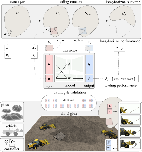
Figure 1: Overview of the model, its development process, and intended usage. First, a dataset of the outcome of different wheel loading actions $\bm{a}$ on a pile with local shape $\bm{h}$ is collected using a simulator. Two models are trained. One model predicts the expected loading performance $\bm{\mathcal{P}}$, in terms of mass, time, and work, given a pile state and an action. Another model predicts the new shape $\bm{h}^{\prime}$ of the pile after the loading is completed. The outcome of a sequence of loading actions on a pile with global state $H$ can be predicted by repeated model inference, given the dig location $\bm{x}$ and heading $\bm{t}$ for each loading.

The feasibility of learning wheel loading predictor models was investigated for accuracy, inference speed, and the required amount of training data. In general, model accuracy can be improved by increasing the input and output dimensions and the number of internal model parameters. However, larger models normally require more training data and may have lower inference speeds. To see the difference, we developed both a high-dimensional and a low-dimensional model using different representations of the pile state. The high-dimensional model takes a well-resolved heightmap of the pile state as input. This may capture many details of the pile surface at the cost of additional model parameters associated with convolutional layers. The low-dimensional model takes a heavily reduced representation of the pile surface, involving only four scalar parameters for its slope and curvature.

The predictor models are trained and evaluated on a dataset from over 10,000 simulated loading cycles performed on gravel piles of variable shape. It is impractical to produce this size of the dataset with field experiments or using coupled multibody and discrete element method (DEM) simulation of large piles of granular material. We used a wheel loading simulator [11, 12] based on contacting 3D multibody dynamics with a real-time deformable terrain model that has been shown to produce digging forces and soil displacements with an accuracy close to that of resolved DEM and coupled multibody dynamics [13]. The simulated wheel loader is equipped with a type of admittance controller [14], parameterized by four action parameters that determine how the boom and bucket actuations respond to the current dig force.

Our main contribution in this paper is developing predictor models for single loading actions given the initial pile state, and investigating how sensitive the model accuracy and the prediction cost are to the model complexity. The models predict the loading outcome, including the resulting pile state, mass, time, and work. The net performance and final pile state from a sequence of loading actions can thus be predicted by repeated model inference. The models shown to be differentiable with respect to the action parameters, which enables the use of gradient-based optimization algorithms. This paper ends by analyzing the models’ predictive properties and speed, leaving the solution of the associated optimization problem to future work.

2 Related work

Data-driven models for predicting bucket-soil interaction have been studied before from several perspectives, including automatic control [15, 16, 17, 18] and motion planning [19, 20]. Model predictive control of earthmoving operations relies on a model to predict the dig force or soil displacement given a control signal acting over some time horizon and the current (and historic) system state. Koopman lifting linearization was used in  [15] for a model predicting the time evolution of the soil forces and effective inertia acting on an excavator bucket given the shape of the soil surface and the position and velocity of the bucket. The model, trained on simulated data, was used for trajectory tracking control with a planning horizon of roughly one second. In [17], a data-driven model for earthmoving dynamics was developed to predict the time evolution of a bulldozer and the terrain surface over a one-second horizon, given the actions and the history of states and actions. The local terrain surface is observed as a heightmap with a regular grid and represented in lower-dimension form using a variational autoencoder (VAE). The dynamics in the reduced representation were learned using recurrent long short-term memory (LSTM) and mixture density neural networks. The model was used to control a blade removing a berm in a simulated environment. A similar approach was used in [18] to predict the time evolution of the soil surface in bucket excavation with a circular trajectory at different depths. For the excavation of rocks, a Gaussian process model was used in [16] to model the interaction dynamics between a bucket, a rock, and the surrounding soil. The experiments were conducted in a laboratory environment using a robotic arm, depth camera, and camera-based tracking of the rock with tracking markers. A limitation of all these models designed for continuous control is that the prediction drifts over time during rollout. To provide useful predictions of the outcome of a loading cycle, they would require real-world observations and re-evaluation at least every second.

Other researchers have developed models to predict the outcome of a wheel loading cycle for trajectory planning. In [20], a model to predict the bucket fill factor from the shape of the pile surface was developed from data collected from 30 simulated loadings using coupled multibody dynamics and DEM. First, the volume of soil swept by a selected bucket trajectory was computed. The predicted fill factor was then computed using a regression model for how the loaded volume relates to the swept volume. In search of optimal loading strategies, a regression Kriging model was developed to predict the outcome of a target bucket trajectory. It had four parameters: target fill factor, dig depth, attack location, and bucket curl [19]. The model output included the loaded mass per time unit, the amount of spillage, and damaging forces on the equipment. Training and validation data included 4,880 simulated cycles of an underground loader digging in piles of coarse rocks confined in a mining drift. None of these models predicted the resulting pile shape, the exerted work, or the loading time.

3 Models for predicting the loading outcome

3.1 Preface and nomenclature

This paper defines loading as starting with a machine heading in direction $\bm{t}$ to dig location $\bm{x}$ in a pile, represented by the current pile state $H$. It ends when the machine has returned to its initial location after digging in, filling the bucket, breaking out, and leaving the pile in a new state $H^{\prime}$. At the dig location $\bm{x}$, a controller for automatic bucket filling is engaged, parametrized by some set of action parameters $\bm{a}$. The loading is performed with some performance $\bm{\mathcal{P}}$, which in this study includes the loaded mass, loading time, and mechanical work. The performance is a consequence of the dynamics of the machine under the selected action $\bm{a}$ and the state of the pile. The expected performance of a loading cycle, indexed by $n\in\mathbb{N}$, is therefore given by some unknown performance predictor function $\bm{\Psi}$. In other words,

$$\widehat{\bm{\mathcal{P}}}_{n}=\bm{\Psi}(H_{n},\bm{x}_{n},\bm{t}_{n},\bm{a}_{n}),$$ (1)

where we use the hat to distinguish predictions from actual values. The net effect of a sequence of $N$ loading cycles is the accumulated outcome of a sequence of loading actions, $\bm{a}_{1},\ldots,\bm{a}_{N}$, applied on a sequence of pile states $H_{1},\ldots,H_{N}$. Each loading transforms the pile from its previous state to the next, $H_{n}\to H^{\prime}_{n}\equiv H_{n+1}$, according to some unknown pile state predictor function $\bm{\Phi}$

$$\widehat{H}^{\prime}_{n}=\bm{\Phi}(H_{n},\bm{x}_{n},\bm{t}_{n},\bm{a}_{n}).$$ (2)

The net outcome of $N$ sequential loading actions is thus given by the sum

$$\widehat{\bm{\mathcal{P}}}_{1:N}\equiv\sum_{n=1}^{N}{\widehat{\bm{\mathcal{P}}}_{n}(\widehat{H}^{\prime}_{n-1},\bm{x}_{n},\bm{t}_{n},\bm{a}_{n})}$$ (3)

with initial pile state $H^{\prime}_{0}=H_{1}$. The predictions are associated with some error, which accumulates over repeated loadings from the same pile. The accumulated error in the pile state and the loading performance over a planning horizon of $N$ cycles are

$$\bm{\mathcal{E}}_{1:N}^{\widehat{H}^{\prime}}\equiv \left\lVert\widehat{H}^{\prime}_{N}-H^{\prime}_{N}\right\rVert,$$ (4)

$$\bm{\mathcal{E}}_{1:N}^{\widehat{\bm{\mathcal{P}}}}\equiv \sum_{n=1}^{N}{\left\lVert\widehat{\bm{\mathcal{P}}}_{n}-\bm{\mathcal{P}}_{n}\right\rVert}.$$ (5)

When solving the problem of finding the sequence of dig locations and loading actions that maximize the net performance $\widehat{\bm{\mathcal{P}}}_{1:N}$, it is beneficial to use gradient-based optimization methods. These require the sought function $\bm{\Psi}$ to be differentiable with respect to $\bm{a}$, and the speed of evaluating the function and its derivative to be sufficiently fast.

3.2 Global and local pile state

We represent the global pile state by a height surface function $z=H(x,y)$ in Cartesian coordinates. This includes not only the shape of the pile but also the surrounding ground, which is assumed to be flat if nothing else is stated. When making sequential predictions, the aim is to accurately predict the global state of the pile, which may take any shape consistent with the physics of the soil. To simplify matters, the predictor models take only the local pile state as input, assuming that the outcome of the loading depends only on the local state and not on the global shape of the pile. A dig location, $\bm{x}=[x,y]$ and heading $\bm{t}$ defines a local frame with basis vectors $\{\bm{e}_{x},\bm{e}_{y},\bm{e}_{z}\}$, where $\bm{e}_{x}$ is aligned with the dig direction, and $\bm{e}_{z}$ is the vertical direction aligned with the gravitational field. We represent the local pile state with a discrete heightmap of $I\times J$ grid cells with the side length $\Delta l$. The heightmap, in the local frame, is

$$h_{ij}=H(\bm{x}-\delta\bm{e}_{x}+i\Delta l\bm{e}_{x}+j\Delta l\bm{e}_{y})-H(\bm{x}-\delta\bm{e}_{x})$$ (6)

with integers $i\in[0,I]$ and $j\in[-J/2,J/2]$ and constant displacement $\delta$ that ensures a certain fraction of the ground in front of the pile is present in the heightmap. A valid dig location is along the edge of the pile. As a condition, we define that the exterior part of the local heightmap should cover a volume less than a small number, $\varepsilon$. That is, $\int_{-l_{y}/2}^{l_{y}/2}\int_{0}^{\delta}H(\bm{x}-x^{\prime}\bm{e}_{x}+y^{\prime}\bm{e}_{y})\text{d}x^{\prime}\text{d}y^{\prime}<\varepsilon$ where $l_{y}$ is the width of the local heightmap.

The simplified problem of predicting the loading outcome, Eqs. (1)-(3), using the local heightmap is

$$\widehat{\bm{\mathcal{P}}}_{n} =\psi(\bm{h}_{n},\bm{a}_{n}),$$ (7)

$$\hat{\bm{h}}^{\prime}_{n} =\phi(\bm{h}_{n},\bm{a}_{n}),$$ (8)

$$\widehat{\bm{\mathcal{P}}}_{1:N} \equiv\sum_{n=1}^{N}{\widehat{\bm{\mathcal{P}}}_{n}(\hat{\bm{h}}^{\prime}_{n-1},\bm{a}_{n})}.$$ (9)

with local predictor functions $\psi$ and $\phi$ for the performance and pile state. The computational process is described in Algorithm 1 and illustrated in Fig. 1. It also involves the intermediate steps $\bm{h}_{n}=\texttt{cutout}(H_{n},\bm{x}_{n},\bm{t}_{n})$ and $H^{\prime}_{n}=\texttt{replace}(H_{n},\bm{x}_{n},\bm{t}_{n},\bm{h}^{\prime}_{n})$ to map the local and global heightmaps. The appropriate size of the local heightmap depends on the size of the volume swept by the bucket and the mechanical properties of the soil.

3.3 Local pile characteristics

As an alternative to representing the local pile state in terms of a heightmap, we introduce a low-dimensional characterization, $\tilde{\bm{h}}\equiv[\theta,\alpha,\kappa_{x},\kappa_{y}]=\texttt{characterize}(\bm{h})$, in terms of four scalar quantities: slope angle $\theta$, incidence angle $\alpha$, longitudinal curvature $\kappa_{x}$, and lateral curvature $\kappa_{y}$. These aim to capture the essence of the local pile shape from the perspective of bucket-filling [21, 22]. First, the mean unit normal $\bm{n}$ is computed from the local heightmap. The slope angle relative to the horizontal plane is then computed $\theta\equiv\cos^{-1}\left[\bm{n}\cdot\bm{e}_{z}\right]$. The incidence angle is the angle between the attack direction $\bm{e}_{x}=\bm{t}/\left\lVert\bm{t}\right\rVert$ and the pile normal projected on the horizontal plane $\bm{n}_{\perp}=\bm{n}-(\bm{n}\cdot\bm{e}_{z})\bm{e}_{z}$, that is, $\alpha\equiv\cos^{-1}(\left[\bm{n}_{\perp}\cdot\bm{e}_{x}\right]/\left\lVert\bm{n}_{\perp}\right\rVert)$. See Fig. 2 for an illustration.

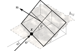
Figure 2: The mean normal $\bm{n}$ defines a slope angle $\theta$ relative to the horizontal plane. The attack angle $\alpha$ is the angle between the dig direction $\bm{t}$ and the normal projected onto the horizontal plane.

Taking inspiration from [23], we calculate the local mean curvature in the $\bm{e}_{x}$ and $\bm{e}_{y}$ directions by fitting a quadratic surface $h(\bm{x})\approx b+\bm{c}^{\text{T}}\bm{x}+\tfrac{1}{2}\bm{x}^{\text{T}}\bm{Q}\bm{x}$ with surface parameters $\bm{Q}=\mathrm{diag}[-\kappa_{x},\enskip-\kappa_{y}]$, $\bm{c}\in\mathbb{R}^{2}$, and $b\in\mathbb{R}$. We chose this sign convention to make the curvatures positive for convex piles, since convexity is recommended for high-performance loading [22].

Initialization: $\widehat{H}^{\prime}_{0}=H_{1}$, $\widehat{\bm{\mathcal{P}}}_{1:N}=\bm{0}$

for $n=1,\ldots,N$ do

       $\bm{x}_{n},\bm{t}_{n}=\texttt{selectDigPose}(\widehat{H}^{\prime}_{n-1})$

       $\bm{h}_{n}=\texttt{cutout}(\widehat{H}^{\prime}_{n-1},\bm{x}_{n},\bm{t}_{n})$

       $\bm{a}_{n}=\texttt{selectAction}(\bm{h}_{n})$

       if high_dim_model then

             $\widehat{\bm{\mathcal{P}}}_{n}=\psi^{\text{high}}(\bm{h}_{n},\bm{a}_{n})$

             $\hat{\bm{h}}^{\prime}_{n}=\phi(\bm{h}_{n},\bm{a}_{n})$

             $\widehat{H}^{\prime}_{n}=\texttt{replace}(\widehat{H}_{n},\bm{x}_{n},\bm{t}_{n},\hat{\bm{h}}^{\prime}_{n})$

            

       else if low_dim_model then

             $\bm{\tilde{h}}_{n}=\texttt{characterize}(\bm{h}_{n})$

             $\widehat{\bm{\mathcal{P}}}_{n}=\psi^{\text{low}}(\bm{\tilde{h}}_{n},\bm{a}_{n})$

             $\widehat{H}^{\prime}_{n}=\texttt{replaceCA}(\widehat{H}_{n},\widehat{\bm{\mathcal{P}}}_{n},\bm{x}_{n},\bm{t}_{n})$

            

      

end for

$\widehat{\bm{\mathcal{P}}}_{1:N}=\sum_{n=1}^{N}{\widehat{\bm{\mathcal{P}}}_{n}}$

Algorithm 1 Long-horizon prediction of the performance and pile state

3.4 Performance predictor model

We developed two different models to predict the loading performance, referred to as the high-dimensional model and the low-dimensional model, respectively. The high-dimensional model, $\psi^{\text{high}}(\bm{h},\bm{a})$, takes the local heightmap $\bm{h}$ as input, while the low-dimensional model, $\psi^{\text{low}}(\tilde{\bm{h}},\bm{a})$, uses the local pile characteristics $\tilde{\bm{h}}$. Both models take the same action parameters $\bm{a}$ as input, and each model outputs a performance vector $\widehat{\bm{\mathcal{P}}}$. The name distinction comes from $\text{dim}(\bm{h})\gg\text{dim}(\tilde{\bm{h}})$. The difference is reflected in the different neural network architectures of the models (Fig. 3). The high-dimensional model uses three convolutional layers and a fully connected linear layer to encode $\bm{h}$ into a latent vector of length 32 before it is concatenated with $\bm{a}$. $\bm{h}$ is interpolated to a size of $32\times 32$ before encoding. The convolutions use ten filters of $3\times 3$ kernels and unit stride with zero-padding. They are followed by batch normalization and max pooling with window size $2\times 2$. The activation function is subject to hyperparameter tuning. The concatenation steps in both $\psi^{\text{high}}$ and $\psi^{\text{low}}$ are followed by a multilayer perceptron (MLP) of identical architectures that are also subject to hyperparameter tuning. We also tested multiple-order polynomial regression and radial basis functions for the low-dimensional model, but did not achieve higher accuracy, and so settled for an MLP because of its ease of implementation and fair comparison.

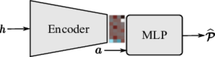
(a) The high-dimensional model $\widehat{\bm{\mathcal{P}}}=\psi^{\text{high}}(\bm{h},\bm{a})$ .

(b) The low-dimensional model $\widehat{\bm{\mathcal{P}}}=\psi^{\text{low}}(\tilde{\bm{h}},\bm{a})$.

Figure 3: Illustration of the two architectures for the performance predictor model. In the high-dimensional model (a), the heightmap is encoded by a convolutional network before being fed with the action vector to an MLP. In the low-dimensional model (b) the pile characteristics and action vector are input directly to a MLP.

3.5 Pile state predictor model

This model is inspired mainly by the work in [18], which combined an autoencoder with an LSTM network to make sequential short-term predictions of excavator soil deformation. Our proposed model consists of three steps using a VAE architecture. First, an encoder network compresses the initial pile state $\bm{h}$ into a lower-dimensional, regularized latent representation $\bm{z}$. Next, given $\bm{z}$ along with the loading action $\bm{a}$ and a scale factor $\Delta h\equiv\max(\bm{h})-\min(\bm{h})$, an MLP predicts the regularized latent representation of the new pile state $\bm{z}^{\prime}$. Last, a decoder network constructs the resulting pile state $\hat{\bm{h}}^{\prime}$ from $\bm{z}^{\prime}$. Fig. 4 illustrates the inference process. We used the same architecture as in [24] for the VAE. The encoder consists of four convolutional layers. Each layer contains filters of size 3$\times$3 with unit stride and zero-padding, followed by max pooling with window size $2\times 2$ and Leaky ReLU activation. The number of filters doubles at every layer. After the convolutions, a fully connected layer compresses the output into a regularized latent representation of size 64. The decoder mirrors the encoder architecture. The MLP has two hidden layers with 1,024 nodes and uses Leaky ReLU activation. These MLP hyperparameters were turned to be optimal. Note that $\bm{h}$ is interpolated to size $64\times 64$ before encoding.

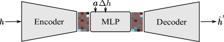
Figure 4: The model architecture of the pile state predictor model combines a variational autoencoder and an MLP for the state transition in latent space.

3.5.1 Post-processing

VAEs are known to produce somewhat blurry images [25]. In our case, this leads to a loss of detail in the decoded pile states. In our preliminary tests, we found that we could improve the prediction accuracy on average by reusing some information from the initial pile state. We interpolate between $\bm{h}$ and $\hat{\bm{h}}^{\prime}$ along the edges to retain the details of the outer area especially. This makes the predicted local pile states blend seamlessly into the global pile state at the replace operation. Fig. 5 illustrates the post-processing.

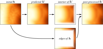
Figure 5: The post-processing interpolates between the interior of the predicted $\hat{\bm{h}}^{\prime}$ and the edges of the initial heightmap $\bm{h}$ to preserve the details along the boundary. The pile in the heightmaps, color-coded by height, was dug from the left.

3.6 Low-dimensional pile state prediction using cellular automata

The low-dimensional predictor model does not have direct access to the local heightmap. Instead, we construct a predictor method that acts directly on the global pile state, called replaceCA in Algorithm 1. It works in two stages. First, the predicted load mass (part of the performance vector $\bm{\mathcal{P}}_{n}$) is removed from the global pile state at the dig location. This is done by computing the corresponding volume and subtracting this from the global pile along a strip as wide as the bucket, starting at $\bm{x}_{n}$ and stretching along $\bm{t}_{n}$. In the second stage, soil mass is redistributed to eliminate any slopes steeper than the set angle of repose. The mass-preserving cellular automata algorithm in [26] is employed, with the “velocity of flowing matter” set to $z_{+}=0.2\Delta l$.

3.7 Delimitations

The predictor models developed in this paper are limited to a single type of soil, namely gravel, which is assumed to be homogeneous. However, the learning process of the predictor models can be repeated for any other soil type supported by the simulator. A more general but computationally costly approach would be to train a predictor model that takes soil parameters as part of the input. This paper does not consider soil spillage on the ground after breaking out with an overfilled bucket. Spillage would affect subsequent performance, either by loss in control precision or traction, or by the need to clear the ground. In this paper, the word “loading” means the bucket-filling phase, including approaching the pile straight ahead and reversing in the opposite direction after the breakout, following the definition in [19]. To account for complete full loading performance, one should incorporate the V-cycle manoeuver, emptying the bucket into the load receiver, and clearing spillage from the ground.

4 Simulator and loading controller

4.1 Simulator

We collected data using a simulator developed in a previous study [11] and recently carefully validated [12]. In brief, the simulator combines a deformable terrain model with a wheel loader model and runs approximately in real-time on a conventional computer. The terrain model, introduced in [13], combines the description of soil as continuous solid, distinct particles, and rigid multibodies. When a digging tool comes in contact with the terrain, the active zone of moving soil is predicted and resolved in terms of particles using DEM. When particles come to rest on the terrain surface, they merge back into the solid soil. The total mass is preserved in all the computational processes. The wheel loader is modeled as a rigid multibody system, matching roughly the dimensions and physical properties of a Komatsu WA320-7. The model has five actuated joints, with hinge motors powering the driveline and steering, and linear motors for the boom and the bucket cylinders. The motors are controlled by specifying a momentaneous joint target speed and force limits. The actuators will run at the set target speed only if the system dynamics and required constraint force do not exceed their respective force limits. The limits are set to match the strength of the real machine [27]. The transmission driveline model includes the main, front, and rear differential couplings to the wheels. The force interaction between the vehicle and the terrain occurs through the tire-terrain and bucket-terrain contacts. The forces on the bucket depend on the shape and amount of active soil, its dynamic state, and mechanical properties, including bulk density, internal friction angle, cohesion, and dilatancy angle. As in [12], these are set to the values 1727 kg/m³, $32^{\circ}$, $0$ kPa, and $8^{\circ}$, which are intended to reflect the properties of dry gravel. The simulations were run with the physics engine AGX Dynamics [28] using a $0.01$ s time-step and terrain grid cell-size of $0.1$ m. Fig. 1 shows images from the wheel loading simulations.

4.2 Loading controller

Assuming the V-shaped motion from a load receiver is neglected, the loading scenario starts with the machine driving at $8$ km/h and toward a pile $5$ m from the target dig location. The bucket is lowered and held level to the ground during the approach. The target drive velocity is kept constant during the bucket-filling phase, although the actual velocity will vary due to digging resistance. Throughout the cycle, the machine maintains the same heading. When the bucket reaches the set dig location $\bm{x}$, the automatic bucket-filling controller is engaged. This controller was inspired by the admittance controller from [14], which regulates the bucket actuator velocity using the measured boom cylinder force. Our admittance controller uses the same method but applies it to both the boom and bucket actuators. The controller determines the target velocities of the boom and bucket cylinders, $v_{\text{bm}}$ and $v_{\text{bk}}$, as follows

$$v_{\text{bm}} =\text{clip}\left(k_{\text{bm}}\left[f_{\text{bm}}/f_{\text{b0}}-\delta_{\text{bm}}\right],0,1\right)v_{\text{bm}}^{\text{max}},$$ (10)

$$v_{\text{bk}} =\text{clip}\left(k_{\text{bk}}\left[f_{\text{bm}}/f_{\text{b0}}-\delta_{\text{bk}}\right],0,1\right)v_{\text{bk}}^{\text{max}},$$ (11)

where $f_{\text{bm}}$ is the momentaneous boom cylinder force. The ramp function has four parameters (velocity gains $k_{\text{bm}}$ and $k_{\text{bk}}$, and force thresholds $\delta_{\text{bm}}$ and $\delta_{\text{bk}}$) that parameterize the behavior of the controller. The actuator max speeds, $v_{\text{bm}}^{\text{max}}$ and $v_{\text{bk}}^{\text{max}}$, and the normalizing boom force $f_{\text{b0}}$ are set using specifications from the manufacturer. The control parameters are collected in the action vector

$$\bm{a}=\left[\delta_{\text{bm}},k_{\text{bm}},\delta_{\text{bk}},k_{\text{bk}}\right].$$ (12)

Parameters $\delta_{\text{bm}}$ and $\delta_{\text{bk}}$ regulate what force magnitude is required to trigger the lift and tilt reactions, while parameters $k_{\text{bm}}$ and $k_{\text{bk}}$ control how rapid the reaction is. Different values of the control parameter thus render different scooping motions, as illustrated by the examples in Fig. 6. The challenge is to select the parameters most appropriate for the local pile state. Note that the controller operates only on the lift and tilt actuators. The vehicle keeps thrusting forward, trying to reach the set target drive velocity. If there is insufficient traction, the wheels may slip.

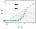
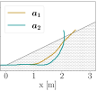
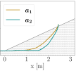
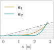
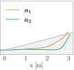
Figure 6: Examples of simulated trajectories using two different sets of action parameters $\bm{a}_{1}=[0.1,1.0,0.1,2.5]$ and $\bm{a}_{2}=[0.5,1.0,0.4,4.0]$ on five piles with slope ranging between $30^{\circ}$ and $10^{\circ}$.

The bucket-filling controller is stopped if the bucket achieves the tilt end position, reaches a penetration depth of $3.2$ m, or breaks out of the initial surface, and if the loading duration exceeds $15$ s. The bucket is then tilted with maximum speed to its end position (if not there already), and the brake is finally applied for at least $0.5$ s to let the agitated soil settle. After that, the vehicle is driven in reverse with a target speed of $8$ km/h, lift $v_{\text{bm}}=0.6v^{\text{max}}_{\text{bm}}$ and tilt $v_{\text{bk}}=0.6v^{\text{max}}_{\text{bk}}$ to reach a boom angle of $-20^{\circ}$, relative to the horizontal axis, and the bucket tilt ends. The scenario ends when the vehicle has reversed $5$ m from the dig location. To simplify time and energy comparison between simulations, they all use the same start and end distance from the dig location and all end with identical boom and bucket angles. The target speeds and force measurements are smoothed using a $0.1$ s moving average to avoid a jerky motion.

5 Data collection and model training

This section describes how data is collected from the simulator and used for learning and evaluating the predictor models.

5.1 Loading outcome

The models were developed to predict the outcome of a loading cycle in terms of the performance $\bm{\mathcal{P}}$ and the resulting local pile state $\bm{h}^{\prime}$ given the initial pile $\bm{h}$ and action $\bm{a}$. The performance is measured using the three essential scalar metrics, namely load mass (tonne), loading time (s), and work (kJ). Hence $\bm{\mathcal{P}}\in\mathbf{R}^{3}$. The load mass is measured as the amount of soil carried by the bucket at the end of each loading cycle. Loading time is the time elapsed between the start and the end of each loading cycle. The work is the energy consumed by the boom and bucket actuators and the forward drive. It is computed as $\int_{0}^{T}\sum_{j}{P_{j}}dt$, where $P_{j}=\max(f_{j}(t)v_{j}(t),0)$ is the power for actuator $j$ with motor force $f_{j}(t)$ and speed $v_{j}(t)$. The work includes the energy required for filling the bucket, breaking out, raising the bucket, and accelerating both the vehicle and soil. Most of the work is lost to frictional dissipation internally in the soil and at the bucket-soil interface. The physics-based simulator accounts for this dissipation. Energy dissipation in the vehicle engine and hydraulics is, however, not included, and should be added if needed.

5.2 Data collection

We collected a total of $10,718$ samples, $\{\bm{h}_{n},\bm{a}_{n},\bm{h}^{\prime}_{n},\bm{\mathcal{P}}_{n}\}_{n=1}^{10718}$, by repeating the loading scenario (Sec. 4.2) in the simulation. First, six different initial piles were prepared, two triangular, two conical, and two wedged with respective slope angles of $20^{\circ}$ and $30^{\circ}$. These are illustrated in Fig. 7. Perlin noise [29] was applied to the surfaces to increase the variability in pile shape. For each of the six initial piles, 30 consecutive loading cycles were simulated. Each loading cycle produced one data point $(\bm{h}_{n},\bm{a}_{n},\bm{h}^{\prime}_{n},\bm{\mathcal{P}}_{n})$. Since the resulting pile state was used as the initial state in the next loading cycle, a variety of piles of different shapes was achieved. This process was repeated 60 times for each of the six seed piles.

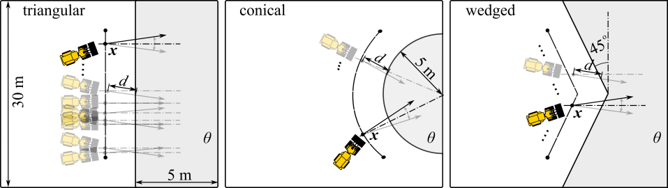
Figure 7: Six initial seed piles are used, triangular, conical, and wedged, with slope angle $\theta$. The dig location $\bm{x}$ and heading are randomized at each loading.

In each simulation, a random dig location was selected, and the wheel loader was positioned at $\bm{x}_{n}$, a distance of 5 m from the pile, and the heading was given a random disturbance of $\pm 10^{\circ}$, see Fig. 7. Each loading used a set of action parameters, $\bm{a}_{n}$, randomly sampled by Latin Hypercube Sampling (LHS) with the ranges $0.0\leq\delta_{\text{bm}},\delta_{\text{bk}}\leq 0.7$ and $0.0\leq k_{\text{bm}},k_{\text{bk}}\leq 5.0$. Note that the actual slope angle $\theta$ and incidence angle $\alpha$ varied according to the dig location because of the Perlin noise.

5.3 Local heightmap settings

We found that the performance and pile state predictor models benefit from using different sizes of the local heightmap and displacement $\delta$ in the dig direction. We used a 3.6 m sided quadratic heightmap discretized by $36\times 36$ grid cells and zero displacement for the performance predictor. The size leaves a margin of $0.5$ m on the sides of the bucket. The pile state predictor needed a larger heightmap to capture the state that the pile finally settles into after the breakout. For this, we used a heightmap with 5.2 m side lengths, discretized in $52\times 52$ cells, and a $1.0$ m displacement.

5.4 Model training

This section describes the training processes of the performance predictor (Sec. 5.4.1) and the pile state predictor model (Sec. 5.4.2), respectively. The models were implemented using PyTorch.

5.4.1 Performance predictor model

The models were trained until convergence with a mean squared error (MSE) loss using the Adam optimizer with a learning rate of $10^{-5}$. Hyperparameter tuning was done via grid search over the number of hidden layers (1, 2, or 3), the number of units ($2^{3},2^{4},\ldots,2^{12}$) in each hidden layer with 0.1 dropout rate, as well as the activation function in fully connected and convolutional layers (Leaky ReLU or Swish [30]). The dataset was first min-max normalized. The training and validation set (split 90/10) was sequentially increased in size from 100 to 9,646 samples, while the test set size was fixed at 1,072 samples.

5.4.2 Pile state predictor models

The pile state predictor model was trained in a two-stage process. First, we trained the VAE to perform heightmap reconstruction. That is, an encoder network compressed the input pile state $\bm{h}$ into a lower-dimensional latent representation $\bm{z}\in\mathbb{R}^{64}$, and a decoder network tried to use it to reconstruct the input pile state. Before training, the heightmaps were rescaled by subtracting the average slope and applying min-max scaling to them individually,

$$\bm{h}_{n} :=\bm{h}_{n}-\frac{1}{N}\sum_{m=1}^{N}\bm{h}_{m}$$ (13)

$$\bm{h}_{n} :=\frac{\bm{h}_{n}-\min(\bm{h}_{n})}{\max(\bm{h}_{n})-\min{\bm{h}}_{n}}.$$ (14)

The standardization in Eq. (13) centers each height distribution around 0 across the entire data set before applying the min-max scaling in Eq. (14). We found this helps to preserve the pile-ground boundary in our reconstructions. The normalization in Eq. (14) makes the VAE agnostic to scale, which we found increases its overall performance. VAE was trained using the Adam optimizer with a learning rate of $10^{-3}$. We used a weighted sum of the elementwise MSE and the Kullback-Leibler Divergence (KLD), $\mathcal{L}_{\mathrm{VAE}}=\mathcal{L}_{\mathrm{MSE}}+0.1\mathcal{L}_{\mathrm{KLD}}$ for the loss function.

In the second training phase, we used the encoder trained in the first phase to encode sampled pile state pairs $(\bm{h},\bm{h}^{\prime})$ into latent pairs $(\bm{z},\bm{z}^{\prime})$. We then trained an MLP with a 0.1 dropout rate for the hidden layers and used the Adam optimizer with a learning rate $10^{-5}$.

The full dataset was used with a split ratio of 80/10/10 in training, validation, and test data for the pile state predictor. Since the wheel loader geometry and actions are left-right symmetric, we applied random reflections to the heightmaps to augment the dataset.

6 Results

The models for predicting the loading performance and resulting pile state were evaluated separately on the hold-out test data. The selected models were finally tested together to predict the outcome of sequential loading.

6.1 Overview of the dataset

First, the general characteristics of the collected dataset were investigated. As expected, we observed a widespread in bucket-tip trajectories because of variability in loading action parameters and pile states (Fig. 8). The loading performance, shown in Fig. 9, is also well distributed in the intervals of 1-4.5 tonne, 7-25 s, and 200-1100 kJ. As expected from a previous study [21], productivity (loaded mass per time unit) is positively correlated with the slope angle and negatively with the incidence angle.

Figure 8: All bucket-tip trajectories in the collected dataset, randomly colored.

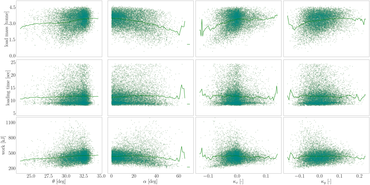
Figure 9: The distribution of the collected performance measurements and how they are correlated with the characteristic pile slope $\theta$, incidence angle $\alpha$, and curvature $\kappa_{x}$ and $\kappa_{z}$. The line is the performance moving average of each characteristics variable.

6.2 Performance predictor model

In total, we developed 480 model instances during the hyperparameter tuning for both the high and low-dimensional performance predictors, $\psi^{\text{high}}$ and $\psi^{\text{low}}$. The models were evaluated using three metrics: mean relative error (MRE), training time, and inference speed. The MRE is relative to the simulation ground truth and is calculated from the average of five distinct training results. The training time was counted as the time per epoch (number of epochs ranging up to about $2,000$), calculating the median over the entire training. The inference speed is measured as the model execution time, taking the average of 1,000 model executions.

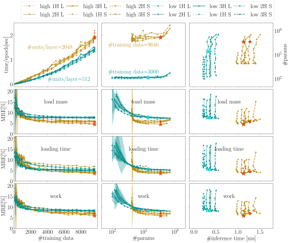
Figure 10: The trend of generalization error (MRE), inference time, and training time (time/epoch) with the number of training/validation data (#training data) and parameters (#params). The parameters are changed by the number of units/layer and the number of hidden layers (H). The activation function used is either Leaky ReLU (L) or Swish (S). Note that the number of units is fixed at 512 for $\bm{\Psi}^{\text{low}}$ and 2048 for $\bm{\Psi}^{\text{high}}$ in the figures of #training data vs. MRE and time/epoch. The number of training/validation data is fixed at 3,000 for $\bm{\Psi}^{\text{low}}$ and 9,646 for $\bm{\Psi}^{\text{high}}$ in the other figures. The filled symbols $\diamond$ and $\star$ identify the models of Swish and Leaky ReLU as the extreme examples of higher inference speed $\bm{\Psi}^{\text{low}}$, and higher accuracy model $\bm{\Psi}^{\text{high}}$. Table 1 shows these specific results.

Fig. 10 shows the effect on the model of changing the amount of training data and the number of model parameters in the MLP. As can be expected, the MRE decreases with increasing size of the dataset and the model, but the accuracy eventually levels out. The best high-dimensional model was achieved when using the full training dataset (9,646 samples). The precise MLP architecture was less important. We selected the MLPs with two hidden layers with $2,048$ units as models of special interest. These are denoted $\psi^{\text{high}}_{\diamond}$ and $\psi^{\text{high}}_{\star}$, where the difference is the use of Swish and Leaky ReLU for activation functions. These models have roughly $10^{7}$ model parameters, including the convolutional layers. The loading performance MRE, listed in Table 1, ranges between 3.5 and 7 % with insignificant dependence on the activation function. For the low-dimensional model, the selected models of special interest, $\psi^{\text{low}}_{\diamond}$ and $\psi^{\text{low}}_{\star}$, are smaller with two hidden layers and $512$ units per layer. This amounts to roughly $5\times 10^{5}$ parameters (no convolutional network is involved). It was trained on a smaller dataset with only 3,000 samples, as there was no significant improvement by adding additional samples. The loading performance MRE for the low-dimensional model saturates in the range of about 5.5-8.5 %, in other words, with 20-70% larger errors than for the high-dimensional model.

The training time and inference time are also shown in Fig. 10 and, for the selected models, in Table 1. The selected low-dimensional model trains about seven times faster and inference runs three times faster than the selected high-dimensional model. The computational overhead of using Swish over Leaky ReLU is marginal.

Table 1: Specific values of the extreme models.

	$\psi^{\text{high}}$		$\psi^{\text{low}}$
	L ReLU	Swish	L ReLU	Swish
mass MRE [%]	$\bm{4.47}$	$\bm{5.70}$	7.77	7.58
time MRE [%]	$\bm{3.61}$	$\bm{4.43}$	5.66	5.41
work MRE [%]	$\bm{5.90}$	$\bm{6.98}$	8.51	8.47
training time [s]	1.9	1.92	$\bm{0.27}$	$\bm{0.27}$
inference time [ms]	1.13	1.27	$\bm{0.31}$	$\bm{0.36}$

It is of interest to see how the errors are distributed in the space of the predictions (Fig. 11). We observe that the relative error (RE) remains comparatively small for high load masses while it increases for the smallest load masses. This suggests that the model is more reliable for high-performing loading actions, which is the general goal, than for low-performing ones.

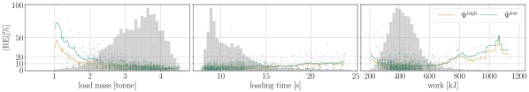
Figure 11: The distribution of relative error over the prediction visualized by a scatter plot and the moving average (curves). The gray histograms show the distribution of the training data.

It is interesting to understand why the model fails occasionally. Therefore, we identified the test samples with the ten worst load mass predictions. These are displayed in Fig. 12 with the local heightmaps. The common factors are a) that the loaded mass is small in the ground truth samples while overestimated by the model and b) that the heightmap is skewed, with most mass distributed on either the left or right side. It is understandable that the low-dimensional model, with only four parameters characterizing the pile state, has more difficulty with these piles as it cannot distinguish between uniform and irregular pile surfaces. That makes accurate load mass prediction difficult for complex pile surfaces.

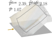
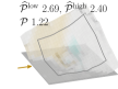
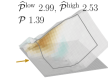
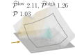
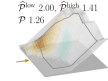
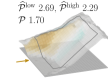
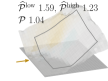
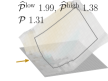
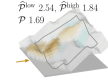
Figure 12: The ten worst load mass predictions of $\psi^{\text{low}}_{\diamond}$. The values shown are the absolute relative error for the low and high-dimensional models and the ground truth load mass. The heightmap of the initial pile state is shown with the grid cells color-coded by the decrease (gold) or increase (cyan) after loading.

6.2.1 Model differentiability

The choice of activation function has a marginal effect on the model’s accuracy, but the quality of gradients also needs to be investigated. To this end, we parameterized a line through the action space using $\bm{a}=\bm{a}_{0}+(\bm{a}_{1}-\bm{a}_{0})s$, with $\bm{a}_{0}=[0.7,0.0,0.0,5.0]^{\text{T}}$, $\bm{a}_{1}=[0.0,5.0,0.7,0.0]^{\text{T}}$, and $s\in[0,1]$. The gradients were calculated by algorithmic differentiation using Pytorch Autograd, with respect to the actions along $\bm{a}(s)$ using the chain rule,

$$\cfrac{\partial\mathcal{P}}{\partial s}=\cfrac{\partial\mathcal{P}}{\partial\bm{a}}\cfrac{\partial\bm{a}}{\partial s}.$$

Fig. 13 shows the result for the selected models. The Swish model produces smoother derivatives than the Leaky ReLU model, which can be expected since Leaky ReLU is not everywhere differentiable, but both appear useful for root-seeking.

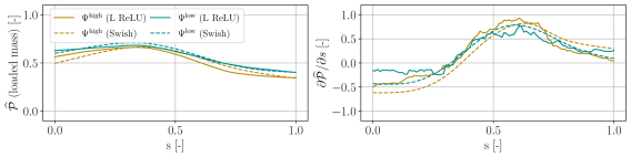
Figure 13: The function values (left) and the Autograd gradients (right) of Leaky ReLU and Swish models with respect to the action $\bm{a}$ along a direction in the action space. The prediction values are normalized.

6.3 Pile state predictor model

The developed pile state predictor model is evaluated by the mean absolute error (MAE) and mean relative error (MRE) of a prediction $\hat{\bm{h}}^{\prime}$ compared to the simulated ground truth heightmap $\bm{h}^{\prime}$. MAE and MRE are calculated in terms of the volume difference of the enclosing surfaces. In detail, the MRE is computed as

$$\text{MRE}=\cfrac{1}{N}\sum_{n}^{N}\varepsilon_{n}^{\text{rel}}=\cfrac{1}{N}\sum_{n}^{N}\cfrac{\sum_{i,j}\lvert\hat{h}_{ij}^{\prime\,n}-h_{ij}^{\prime\,n}\rvert\Delta l^{2}}{\sum_{i,j}\lvert h_{ij}^{\prime\,n}\rvert\Delta l^{2}},$$ (15)

where the volume of each cell, indexed by $ij$, is calculated between the surface and the extended ground plane in the grid. MAE is the same calculation except for the volume normalization. The results are summarized in Table 2. The MAE of misplaced volume constitutes roughly 25 % of the bucket capacity but only 3 % of the volume under the local heightmap. The post-processing step reduces the MAE from 0.84 to 0.75 m³ , with insignificant overhead in inference time. The improvement by the post-processing can also be seen from the distribution of the errors in Fig. 14.

Table 2: Test results of the pile state predictor model, with and without post-processing described in Sec. 3.5.1.

p-p	MAE [m3]	MRE [%]	inference time [ms]
on	0.75	3.04	4.51
off	0.84	3.41	4.48

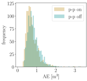
(a)

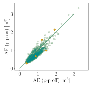
(b)

Figure 14: (a) The distribution of the prediction test error and (b) the AE (p-p off)-AE (p-p on) plot. The five points of interest marked by diamonds ($\diamond$) in (b) are visualized in Fig. 15.

Fig. 15 visualizes five selected test predictions, marked by diamonds in Fig. 14(b).

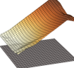
ct-.15in$\bm{h}$ ct-.15inreconstr. $\bm{h}$ ct-.15in$\bm{h}^{\prime}$ ct-.15in$\hat{\bm{h}}^{\prime}$ p-p off ct-.15in$\hat{\bm{h}}^{\prime}$ with p-p on

(a) test data #288, AE (p-p on):0.28, AE (p-p off):0.38.

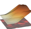
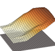
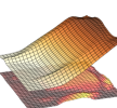
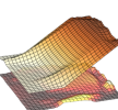
(b) test data #646, AE (p-p on):2.13, AE (p-p off):1.92.

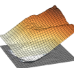
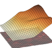
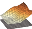
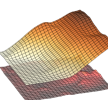
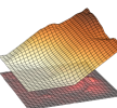
(c) test data #388, AE (p-p on):0.68, AE (p-p off):0.88.

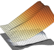
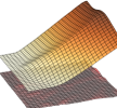
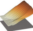
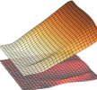
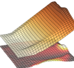
(d) test data #142, AE (p-p on):1.57, AE (p-p off):1.22.

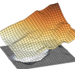
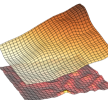
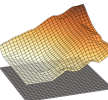
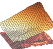
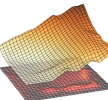
(e) test data #1034, AE (p-p on):0.98, AE (p-p off):1.45.

Figure 15: Samples of initial pile state $\bm{h}$ and the corresponding resulting ground truth pile state $\bm{h}^{\prime}$ and model predictions $\hat{\bm{h}}^{\prime}$, with and without post-processing. The VAE reconstruction capability is included in the second column. Samples (a) have small errors in the test data set, (b) have large errors, and (c) are close to the median. In samples (d) and (e), the post-processing increases and decreases the errors, respectively. The surface under the pile shows the absolute difference compared to the ground truth final pile state except that only in the second column, it is compared to the initial pile state.

Overall, the predicted pile surfaces look reasonable compared to the ground truth. We find that the model performance tends to be better when the initial pile has a smooth, regular shape, which is to be expected as the VAE decoder tends to produce smooth outputs. Examples of the smoothness issue can be seen in the reconstruction column in Fig. 15.

Post-processing is most beneficial in cases where the initial state is irregular and when there is little change at the boundary (Fig. 15(e)). When the initial pile is smooth with a uniform slope close to the angle of repose, loading will induce avalanches that affect the pile state at the rear boundary. This explains why the AE is sometimes increased by post-processing (Fig. 15(d)).

With the selected soil properties (gravel), the resulting pile shape is not highly sensitive to variations in action with equal load mass. Nonetheless, our model can correctly capture some of the nuanced differences caused by different actions. For example, we expect larger deformations when the controller uses slow tilting and lifting, as this gives the wheel loader time to dig deeper into the pile. For all pile states we studied in more detail, we found that the pile state predictor appears to depend smoothly on the action parameters. That is, small changes in action never result in big differences in the output pile shape. Appendix B provides examples of differences in prediction from different input actions.

6.4 Sequential loading predictions

This section demonstrates 40 sequential loading predictions by both the high and low-dimensional models and compares the net outcome $\widehat{\bm{\mathcal{P}}}_{1:N}$ to the simulation ground truth. The simulation and the predictor models start with the same initial pile state, $H_{1}$, and use identical sequences of the dig location, heading, and action parameters, $\{\bm{x}_{n},\bm{t}_{n},\bm{a}_{n}\}_{n=1}^{40}$. The initial pile is the one shown in Fig. 1. Fig. 16 shows the selected headings and dig locations, which are around the left bottom region in the pile. The actions were picked randomly from the training data set. The simulated sequential loading can be seen in Supplementary Video 1. The performance predictor $\psi^{\text{high}}_{\diamond}$ is used together with the pile state predictor $\phi$ for high-dimensional model predictions. The low-dimensional performance predictor $\psi^{\text{low}}_{\diamond}$ is combined with the cellular automata model replaceCA to predict the next pile state.

The evolution of the pile is shown in Fig. 16 and in Supplementary Video 2. The accumulated load mass, time, work, and residual pile volume are summarized in Table 3.

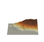
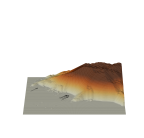
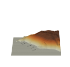
(a) Ground truth

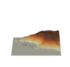
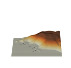
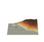
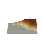
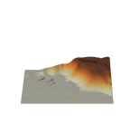
(b) Sequential prediction (high-dimensional model)

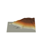
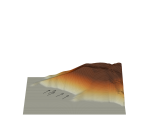
(c) Sequential prediction (low-dimensional model plus replaceCA)

Figure 16: Pile state evolution after every five sequential loadings. The models predict the change in pile state using identical dig locations and the directions (indicated by arrows), and action parameters as the ground truth.

Table 3: The accumulated load mass, time, work, and residual pile volume during sequential loading, GT stands for ground truth.

	$\widehat{\mathcal{P}}_{1:N}$									$\widehat{H}^{\prime}_{N}$
	load mass [tonne]			loading time [s]			work [MJ]			pile volume [m3]
$N$	GT	$\Psi^{\text{high}}$	$\Psi^{\text{low}}$	GT	$\Psi^{\text{high}}$	$\Psi^{\text{low}}$	GT	$\Psi^{\text{high}}$	$\Psi^{\text{low}}$	GT	$\Phi$	rep.CA
5	14.7	15.7	16.1	55.8	53.2	54.5	2.0	2.0	2.0	768.6	765.9	767.7
10	28.2	31.5	31.3	106.1	101.0	101.9	4.1	3.9	3.8	760.7	755.9	758.8
15	40.8	45.3	47.0	161.1	155.4	154.5	6.5	6.1	6.0	753.3	745.6	749.7
20	56.8	62.0	64.4	218.0	210.8	208.1	8.9	8.5	8.3	744.0	728.7	739.5
25	71.0	75.4	80.6	273.7	265.7	260.2	11.1	10.6	10.4	735.7	714.7	730.1
30	86.1	90.5	96.6	327.3	318.7	308.9	13.2	12.8	12.4	726.9	700.1	720.7
35	101.4	106.3	114.3	389.4	385.1	369.9	15.7	15.3	14.6	718.0	679.1	710.4
40	116.0	118.6	130.9	443.0	441.9	418.8	17.9	17.4	16.6	709.5	664.2	700.6

The errors accumulate over time, as is made clear in Fig. 17. While the pile state prediction error for the low-dimensional model grows at a nearly constant rate, the growth rate of the high-dimensional model is more irregular, starting at a lower rate but growing more rapidly after 15 sequential loadings. The loaded mass error grows nearly linearly and roughly at the same rate for both models. Also, the error in loading time and work grows mainly linearly. The models follow the same trend.

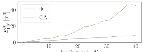
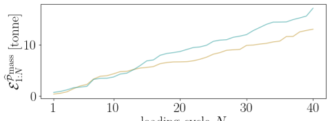
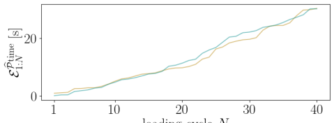
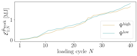
Figure 17: The evolution of the prediction errors during sequential loading.

The high dimensional model uses $\Phi$ for the local pile state prediction, making no change outside the local heightmap as discussed in Sec. 3.5. The accumulated error eventually leads to a predicted pile state with a slope steeper than the angle of repose (Fig. 16).

The accumulated inference time of the high and low-dimensional models was also measured. The high-dimensional model took 0.3 s in total. The low-dimensional model took 0.01 s, but the time for replaceCA to compute the resulting heightmap must be added, for a total of 44.3 s. However, the implementation of replaceCA was not optimized or adapted for GPU computing, so the comparison is unfair.

To summarize, the high-dimensional model was better for shorter time horizons, but the low-dimensional model was more robust for longer horizons. The robustness would be the same if the high-dimensional model used the cellular automata in place of the pile state predictor but with the additional computational cost.

7 Discussion

7.1 Feasibility

The relatively small errors of single loading prediction, 3–8.5 %, are encouraging but do not guarantee that the method is practically useful in its current form. The model is particular to the specific wheel loader and soil, which was homogeneous gravel, of the simulator. Consequently, a new model needs to be trained for each combination of wheel loader model and soil type unless this is made part of the model input. There is a greater need for automation solutions for more complex soils such as blasted rock or highly cohesive media than for homogeneous gravel. Although these materials can be numerically simulated, the problem of learning predictor models may be harder and require different data, as discussed for the loading process in [7]. For blasted rock, the local rock fragmentation probably needs to be included in the model input. On the other hand, the level of accuracy needed ultimately depends on the specific application and the prediction horizon required.

It is an attractive option to train on actual field data (rather than simulated data) to eliminate any simulation bias. That would entail collecting data from several thousand loadings with variations in pile shape and action parameters. This would be demanding but is not unrealistic given the number of vehicles (of the same model) that are in operation around the world. If all were equipped with the same bucket-filling controller, it would ultimately be a question of instrumenting these machines and sites to scan the pile shape before and after loading, and tracking the vehicle’s motion and force measurements.

Long-horizon planning of sequential loading requires long rollouts of repeated model inference. The error accumulation in the pile state predictor model (Fig. 17) might then become an obstacle. If that is the case, the pile state predictor can be replaced with mass removal and cellular automata (replaceCA), as described in Sec. 3.6. Then, replaceCA will likely be the computational bottleneck. In our implementation, the replaceCA was about 200 times slower than model inference, about 1 s versus 5 ms per loading. An optimized implementation of the replaceCA can probably be an order of magnitude faster. Also, the replaceCA could be applied as a post-processor to the pile state predictor to force the pile state to be consistent with the proper angle of repose. If the post-processor is only occasionally needed, instead of after each pile state prediction, the computational overhead may be marginal.

7.2 Applications

We envision that the prediction models can be used in several different ways. They can be used to select the next loading action of an autonomous wheel loader or to plan the movement of both wheel loaders and haul trucks in a way that is optimal for coordinating multiple loading and hauling vehicles with the multi-objective goal of executing individual tasks efficiently while not obstructing the work of the other machines. If the problem of optimal sequential planning is computationally intractable, the prediction models can be useful in developing good planning policies, for instance, using model-based reinforcement learning.

7.3 Diggability map

The model can also be used for operator support. We illustrate this by creating diggability maps, where the model is inferred around the entire edge of a pile. The result, illustrated in Fig. 18, reveals the most favorable dig locations. The map was created by using $\bm{\Psi}^{\text{high}}_{\diamond}$ to predict the performance using a fixed action $\bm{a}=[0.68,4.51,0.17,4.46]$ at 150 dig locations along the local normal direction. The map highlights the regions with higher pile angles where the loaded volume would be relatively high and would be dug with lower energy cost. Some bulges are mapped as low-performance regions. Diggability maps may be produced using a search algorithm for the locally optimal heading and loading action.

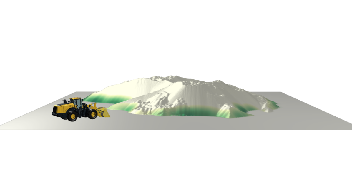
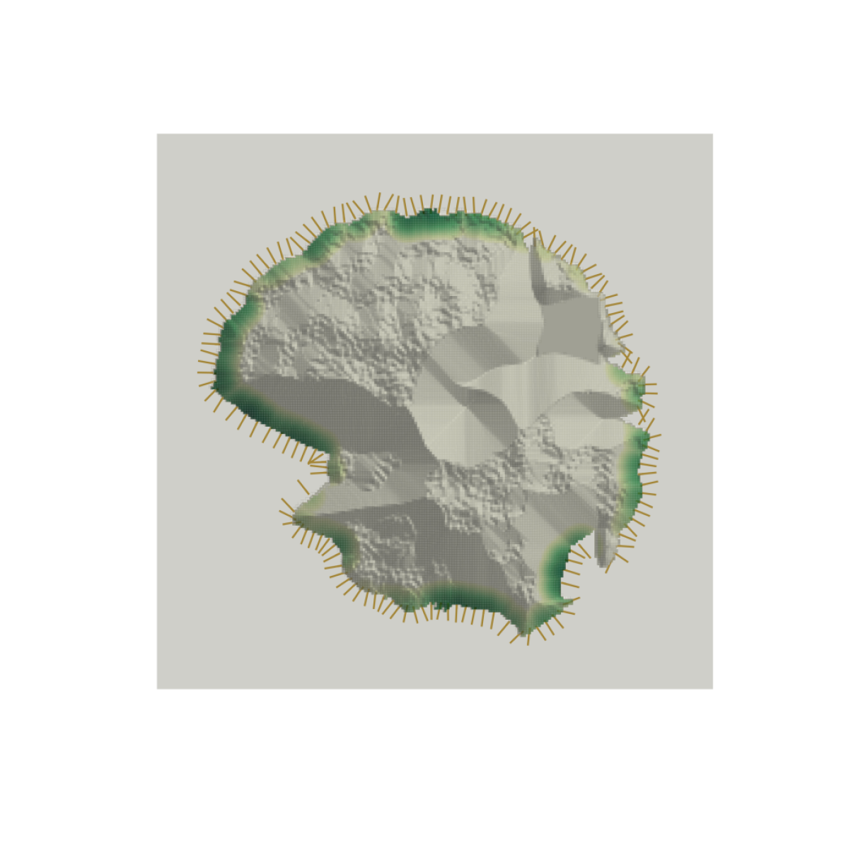
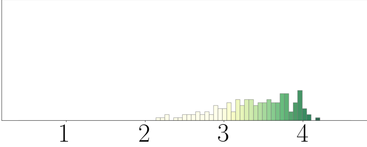
(a) Load mass [tonne].

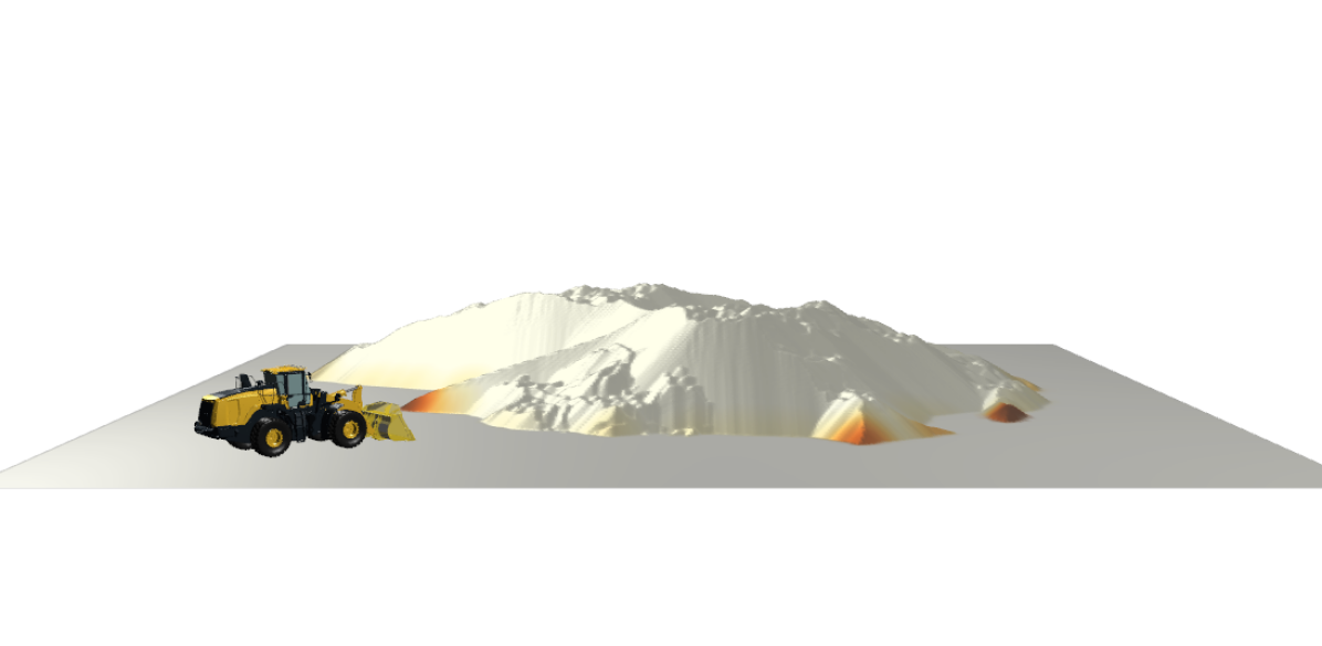
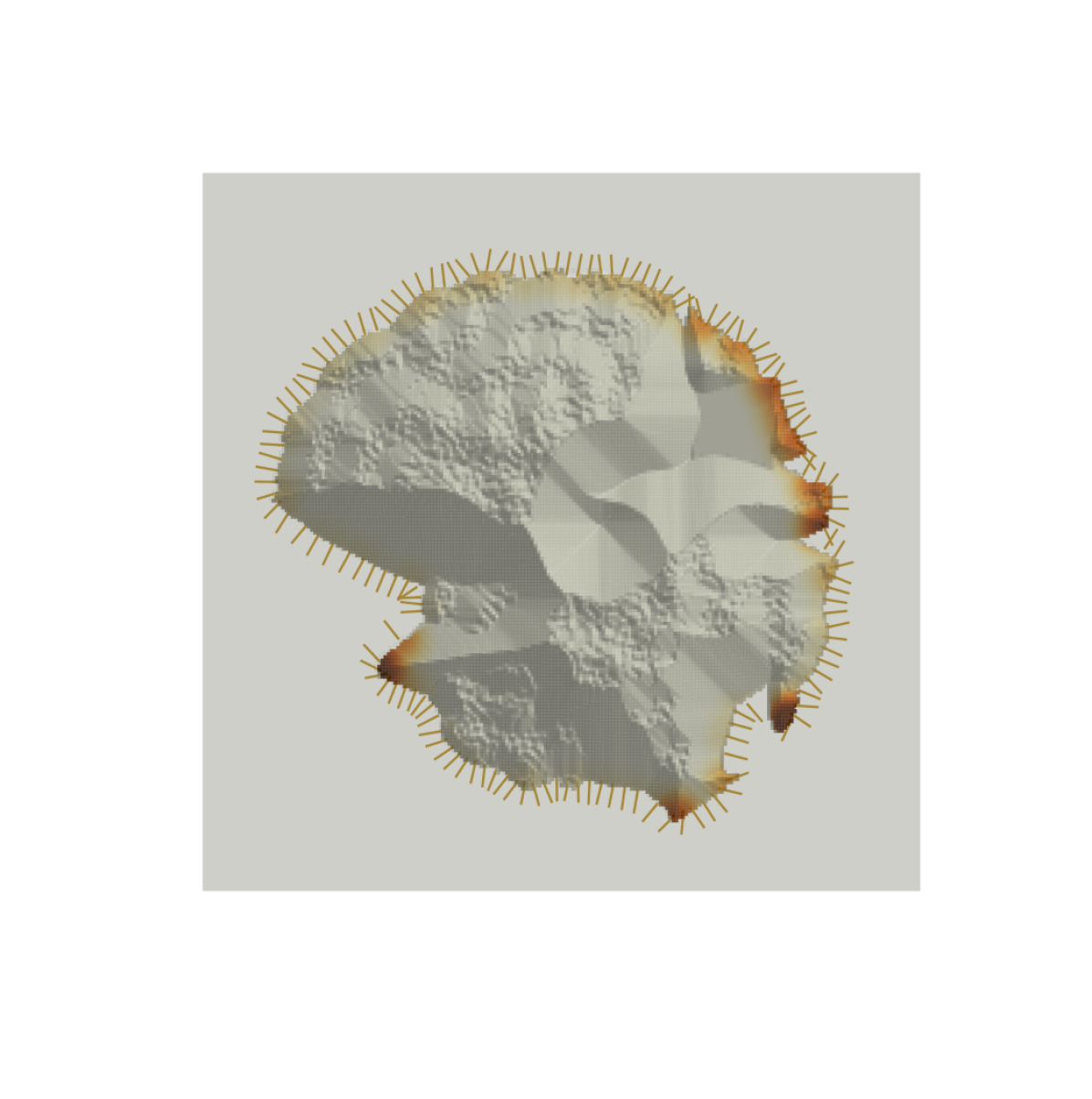
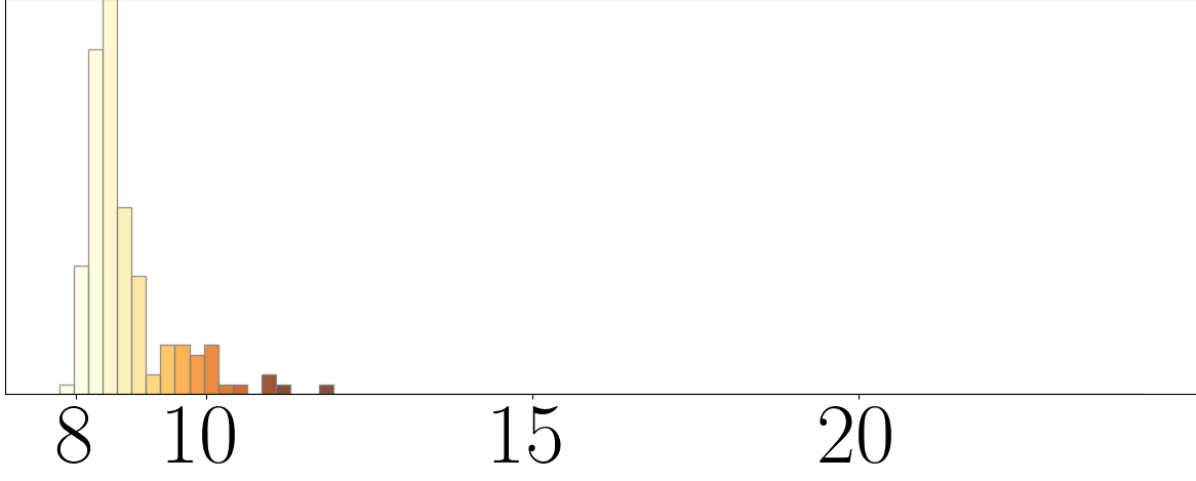
(b) Time [s].

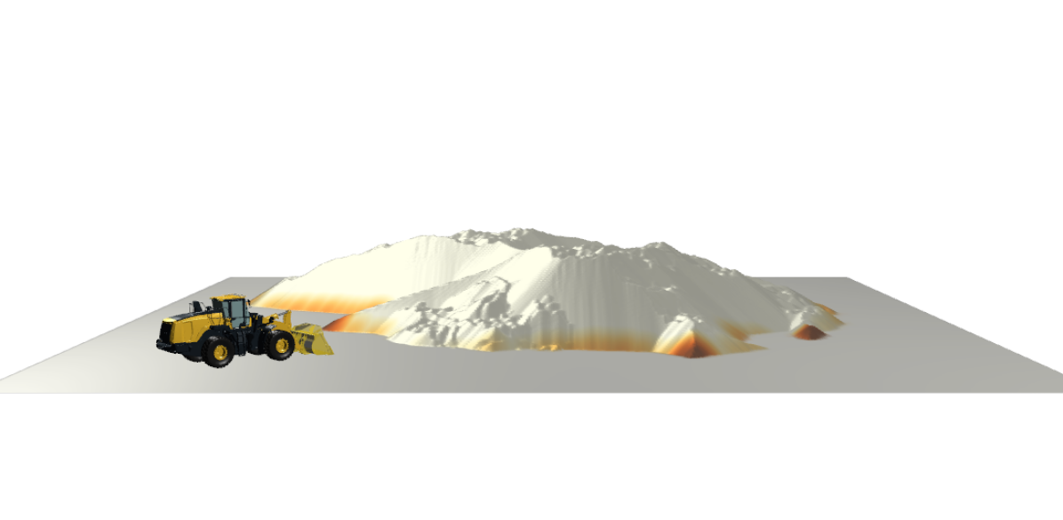
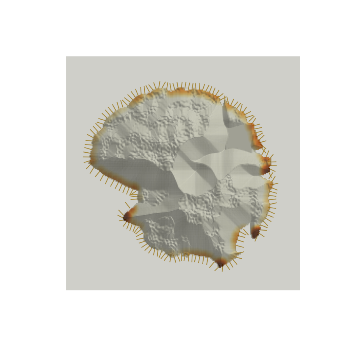
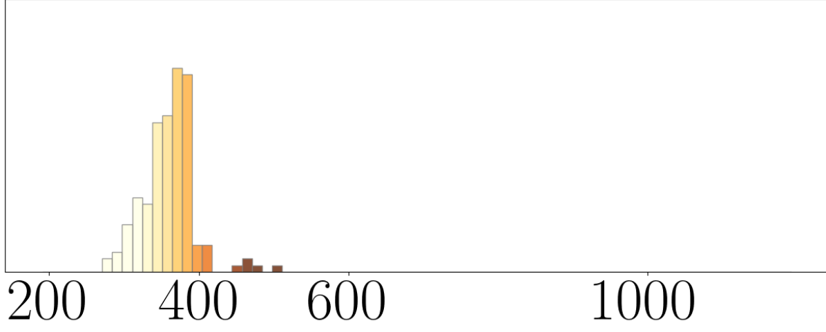
(c) Work [kJ].

Figure 18: Diggability maps that show the predicted loaded mass, time, and work at 150 locations with normal headings, indicated by the lines around the edge. The color coding is explained by the histograms for each of the predicted quantities.

8 Conclusion

This paper shows the feasibility of learning models to predict the outcome of a loading given the local shape of the pile and the choice of control parameters for automatic bucket-filling. The models should be applicable for automatic planning and control of high-performance wheel loading. Future research should focus on handling more complex materials and testing the use of these models in optimal planning. This will help to understand the specific requirements on model accuracy and inference speed.

Appendix A

Supplementary data to this article can be found online at http://umit.cs.umu.se/wl-predictor/.

Appendix B Action dependence of pile state predictions

Here we show the impact of using different actions as input to $\bm{\Phi}$.

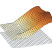
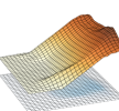
ct-.1in$\bm{p}$ ct-.1in$\hat{\bm{p}}^{\prime}(\bm{a}_{1},\bm{p})$ ct-.1in$\hat{\bm{p}}^{\prime}(\bm{a}_{2},\bm{p})$ ct-.1in$\hat{\bm{p}}^{\prime}(\bm{a}_{3},\bm{p})$

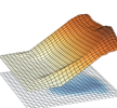
(a) The pre pile state $\bm{p}_{0}$ (from test data #0).

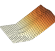
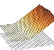
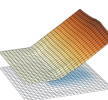
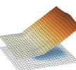
(b) The pre pile state $\bm{p}_{10}$ (from test data #10).

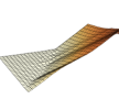
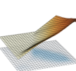
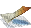
(c) The pre pile state $\bm{p}_{100}$ (from test data #100).

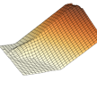
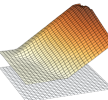
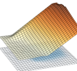
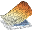
(d) The pre pile state $\bm{p}_{200}$ (from test data #200).

Figure 19: Pile state predictions with different actions $\bm{a}$=[$t_{\text{bm}},k_{\text{bm}},t_{\text{bk}},k_{\text{bk}}$]: $\bm{a}_{1}$=[0.1, 4.0, 0.1, 4.0] (fast lift/fast tilt), $\bm{a}_{2}$=[0.5, 0.1, 0.1, 4.0] (slow lift/fast tilt), and $\bm{a}_{3}$=[0.5, 0.1,0.5, 0.1](slow lift/slow tilt). Error surfaces show the absolute difference compared to the ground truth pre pile state.

References

- [1] Siddharth Dadhich, Fredrik Sandin, Ulf Bodin, Ulf Andersson, and Torbjörn Martinsson. Adaptation of a wheel loader automatic bucket filling neural network using reinforcement learning. In 2020 International Joint Conference on Neural Networks (IJCNN), pages 1–9, 2020.
- [2] Osher Azulay and Amir Shapiro. Wheel loader scooping controller using deep reinforcement learning. IEEE Access, 9:24145–24154, 2021.
- [3] Heshan Fernando and Joshua Marshall. What lies beneath: Material classification for autonomous excavators using proprioceptive force sensing and machine learning. Automation in Construction, 119:103374, 2020.
- [4] Sofi Backman, Daniel Lindmark, Kenneth Bodin, Martin Servin, Joakim Mörk, and Håkan Löfgren. Continuous control of an underground loader using deep reinforcement learning. Machines, 9(10), 2021.
- [5] Daniel Eriksson and Reza Ghabcheloo. Comparison of machine learning methods for automatic bucket filling: An imitation learning approach. Automation in Construction, 150:104843, 2023.
- [6] Eric Halbach, Joni Kämäräinen, and Reza Ghabcheloo. Neural network pile loading controller trained by demonstration. In 2019 International Conference on Robotics and Automation (ICRA), pages 980–986, 2019.
- [7] Carl Borngrund, Fredrik Sandin, and Ulf Bodin. Deep-learning-based vision for earth-moving automation. Automation in Construction, 133:104013, 2022.
- [8] S. Singh and R. Simmons. Task planning for robotic excavation. In Proceedings of the IEEE/RSJ International Conference on Intelligent Robots and Systems, volume 2, pages 1284–1291, 1992.
- [9] Ahmad Hemami and Ferri Hassani. An overview of autonomous loading of bulk material. pages 405–411, Austin, USA, June 2009. International Association for Automation and Robotics in Construction (IAARC).
- [10] Reno Filla and Bobbie Frank. Towards finding the optimal bucket filling strategy through simulation. In Proceedings of 15: th Scandinavian International Conference on Fluid Power, June 7-9, 2017, Linköping, Sweden, number 144, pages 402–417, 2017.
- [11] Koji Aoshima, Martin Servin, and Eddie Wadbro. Simulation-based optimization of high-performance wheel loading. Proceedings of the 38th International Symposium on Automation and Robotics in Construction (ISARC), Dubai, UAE., 2021.
- [12] Koji Aoshima and Martin Servin. Examining the simulation-to-reality gap of a wheel loader digging in deformable terrain. arXiv preprint arXiv:2310.05765, 2023.
- [13] Martin Servin, Tomas Berglund, and Samuel Nystedt. A multiscale model of terrain dynamics for real-time earthmoving simulation. Advanced Modeling and Simulation in Engineering Sciences, 8(1):1–35, 2021.
- [14] A. Dobson, J. Marshall, and J. Larsson. Admittance control for robotic loading: Design and experiments with a 1-tonne loader and a 14-tonne load-haul-dump machine. Journal of Field Robotics, 34(1):123–150, 2017.
- [15] Filippos E. Sotiropoulos and H. Harry Asada. Dynamic modeling of bucket-soil interactions using koopman-dfl lifting linearization for model predictive contouring control of autonomous excavators. IEEE Robotics and Automation Letters, 7(1):151–158, 2022.
- [16] Filippos E. Sotiropoulos and H. Harry Asada. Autonomous excavation of rocks using a gaussian process model and unscented kalman filter. IEEE Robotics and Automation Letters, 5(2):2491–2497, 2020.
- [17] W. Jacob Wagner, Katherine Driggs-Campbell, and Ahmet Soylemezoglu. Model learning and predictive control for autonomous obstacle reduction via bulldozing. In 2022 IEEE/RSJ International Conference on Intelligent Robots and Systems (IROS), pages 6531–6538, 2022.
- [18] Yuki Saku, Masanori Aizawa, Takeshi Ooi, and Genya Ishigami. Spatio-temporal prediction of soil deformation in bucket excavation using machine learning. Advanced Robotics, 35(23):1404–1417, 2021.
- [19] Daniel M. Lindmark and Martin Servin. Computational exploration of robotic rock loading. Robotics and Autonomous Systems, 106:117–129, 2018.
- [20] Shaojie Wang, Shengfeng Yu, Liang Hou, Binyun Wu, and Yanfeng Wu. Prediction of bucket fill factor of loader based on three-dimensional information of material surface. Electronics, 11(18), 2022.
- [21] S. P. Singh and R. Narendrula. Factors affecting the productivity of loaders in surface mines. International Journal of Mining, Reclamation and Environment, 20(1):20–32, 2006.
- [22] S. Singh and H. Cannon. Multi-resolution planning for earthmoving. In Proceedings. 1998 IEEE International Conference on Robotics and Automation (Cat. No.98CH36146), volume 1, pages 121–126 vol.1, 1998.
- [23] Martin Magnusson, Tomasz Kucner, and Achim J. Lilienthal. Quantitative evaluation of coarse-to-fine loading strategies for material rehandling. In 2015 IEEE International Conference on Automation Science and Engineering (CASE), pages 450–455, 2015.
- [24] N. Kuchur. Landscape generator (github repository). https://github.com/nikitakuchur/landscape-generator, 2021.
- [25] Diederik P Kingma, Max Welling, et al. An introduction to variational autoencoders. Foundations and Trends® in Machine Learning, 12(4):307–392, 2019.
- [26] Marta Pla-Castells, I García, and Rafael J Martínez. Approximation of continuous media models for granular systems using cellular automata. In International Conference on Cellular Automata, pages 230–237. Springer, 2004.
- [27] Komatsu Ltd. WA320-7, February 2017.
- [28] Algoryx Simulations. AGX Dynamics, August 2023.
- [29] Ken Perlin. An image synthesizer. 19(3), 1985.
- [30] Prajit Ramachandran, Barret Zoph, and Quoc V. Le. Searching for activation functions. 2017.