Partial continuum limit of the 2D Hubbard model

Abstract

An effective quantum field theory of the 2D Hubbard model on a square lattice near half-filling is presented and studied. This effective model describes so-called nodal- and antinodal fermions, and it is derived from the lattice model using a certain partial continuum limit. It is shown that the nodal fermions can be bosonized, which leads to spin-charge separation and a 2D analogue of a Wess-Zumino-Witten model. A bosonization formula for the nodal fermion field operator is obtained, and an exactly solvable model of interacting 2D fermions is identified. Different ways of treating the antinodal fermions are also proposed.

Remark added on September 20, 2023: This paper was included in the PhD thesis of the first author, who defended his PhD on December 16, 2011 (this thesis: “Fermions in two dimensions and exactly solvable models,” is available on http://kth.diva-portal.org/). We planned to publish this paper, but for some reason or another this did not happen then.

We make this paper available on the arXiv in the form it was on August 14, 2012 (this is a slight update of the version that appeared in the above-mentioned PhD thesis).

1 Introduction

Advancing our computational understanding of the Hubbard model [1, 2, 3] is an important but challenging problem in the theory of many-electron systems. As one of the minimal models for strongly correlated electrons, its ground state is believed to describe various charge-ordered-, magnetic- and superconducting phases for different parameter values and spatial dimensionality [4, 5]. The Hamiltonian can be represented as

$$H_{{\text{Hubb}}}^{\phantom{{\dagger}}}=-\sum\limits_{\alpha=\uparrow,\downarrow}\sum\limits_{i,j}t_{ij}^{\phantom{{\dagger}}}c_{i,\alpha}^{\dagger}c_{j,\alpha}^{\phantom{{\dagger}}}+U\sum\limits_{i}n_{i,\uparrow}n_{i,\downarrow}$$ (1)

with operators $c_{i,\alpha}^{\dagger}$ and $c_{i,\alpha}^{\phantom{{\dagger}}}$ describing the creation- and annihilation of a fermion with spin projection $\alpha$ at lattice site $i$, $n_{i,\alpha}=c_{i,\sigma}^{\dagger}c_{i,\sigma}^{\phantom{{\dagger}}}$ the corresponding density operators, $U\geq 0$ the strength of the screened Coulomb repulsion, and $t_{ij}$ the hopping matrix elements. Of particular interest for the high-Tc problem of the cuprate superconductors [6, 7, 8] is the two-dimensional (2D) model on a square lattice, which is the focus of the present paper. At half-filling and sufficiently large $U$, there is by now compelling evidence that the model is a Mott insulator [9] with strong antiferromagnetic correlations, as seen for example in rigorous Hartree-Fock- [10, 11] and quantum Monte Carlo studies [12, 13]. Less is known away from half-filling. Numerical Hartree-Fock studies find a plethora of inhomogeneous solutions like polarons, different types of domain walls or stripes, vortex-like structures and ferromagnetic domains; see [14] and references therein. Furthermore, renormalization group studies at weak coupling show Fermi-liquid behavior far from half-filling [15], and strong tendencies towards antiferromagnetism and $d$-wave superconductivity close to half-filling [16, 17, 18, 19, 20]; similar results are obtained from quantum cluster methods [21, 22]. Still, few definitive conclusions can be drawn for arbitrary coupling strength.

This level of uncertainty may be contrasted with the corresponding situation in one dimension. The 1D Hubbard model with nearest-neighbor hopping is integrable and can be solved exactly using Bethe ansatz; see [23] and references therein. More general 1D lattice models of fermions can be successfully studied using numerical methods, e.g. the density matrix renormalization group [24]. An alternative approach is to perform a particular continuum limit away from half-filling that leads to a simplified model that can be studied by analytical methods. This limit involves linearising the tight-binding band relation at the non-interacting Fermi surface points and “filling up the infinite Dirac sea of negative energy states”. For spinless fermions one obtains the (Tomonaga-)Luttinger model [25, 26], which can be solved using bosonization [27]; in particular, all thermodynamic Green’s functions can be computed [28, 29, 30, 31, 32, 33, 34]. Generalizing to arbitrary interacting fermion models away from half-filling leads to the notion of the Luttinger liquid [35] – the universality class of gapless Fermi systems in one dimension (see e.g. [36] for review). Furthermore, spinfull systems like the 1D Hubbard model can be studied using both abelian- and non-abelian bosonization, with the latter leading to a Wess–Zumino–Witten-type (WZW) model [37, 38]. We note that bosonization has a rigorous mathematical foundation, see e.g. [39, 40].

The idea of applying bosonization methods in dimensions higher than one goes back to pioneering work of Luther [41], and was popularized by Anderson’s suggestion that the Hubbard model on a square lattice might have Luttinger-liquid behavior away from half-filling [42]. Consider for example a gapless system with a square Fermi surface. Let $k_{\parallel}$ and $k_{\perp}$ denote fermion momenta parallel and perpendicular, respectively, to a face of the square. Following [41], one would treat $k_{\parallel}$ as a flavor index, extend $k_{\perp}$ to be unbounded, and fill up the Dirac sea such that all states $k_{\perp}<0$ are filled. The system can then be bosonized by the same methods used in one dimension. Unfortunately, in this approach only density operators with momentum exchange in the perpendicular direction behave as bosons, while operators with exchange in the parallel direction do not have simple commutation relations. Yet, Mattis [43] proposed a 2D model of spinless fermions with density-density interactions, containing momentum exchange in all directions, that he claimed was solvable using bosonization. The Hamiltonian of Mattis’ model had a kinetic energy term with a linear tight-binding band relation on each face of a square Fermi surface, and with a constant Fermi velocity $v_{F}$ along each face. Mattis rewrote the kinetic energy as a quadratic expression in densities using a generalized Kronig identity, and the Hamiltonian was then diagonalized by a Bogoliubov transformation.

The exact solubility of Mattis’ model can be understood in light of more recent work of Luther [44] in which he studied a model of electrons with linear band relations on a square Fermi surface: A notable difference to the 1D case is the huge freedom one has in choosing the accompanying flavor indices when bosonizing. In particular, one may do a Fourier transformation in the $k_{\parallel}$-direction and then bosonize using a new index flavor $x_{\parallel}$. In this way, Luther obtained density operators that indeed satisfy 2D boson commutation relations. The price one has to pay for solubility is that $v_{F}$ needs to be constant on each face, i.e. it cannot depend on $k_{\parallel}$. The properties of Luther’s model were further investigated in [45, 46]. We also mention Haldane’s phenomenological approach to bosonization in higher dimensions [47], which has been further pursued by various groups [48, 49, 50], and functional integral approaches to bosonization [51, 52]; none of these will be followed here.

Returning to the 2D Hubbard model, consider momentarily the half-filled square lattice with nearest-neighbor (nn) hopping only. The tight-binding band relation relevant in this case is $\epsilon({\bf k})=-2t[\cos(k_{1})+\cos(k_{2})]$, which gives a square (non-interacting) Fermi surface at half-filling. The functional form of $\epsilon({\bf k})$ varies significantly over this surface: In the so-called nodal regions of the Brillouin zone near the midpoints $(\pm\pi/2,\pi/2)$ and $(\pi/2,\pm\pi/2)$ of the four faces, the band relation is well represented by a linear approximation in the perpendicular direction to each face. In contrast, at the corner points $(\pm\pi,0)$ and $(0,\pm\pi)$ in the so-called antinodal regions, $\epsilon({\bf k})$ has saddle points. This makes taking a constant Fermi velocity along each face a questionable approximation. Furthermore, we know that the van-Hove singularities associated with these saddle points, and the nesting of the Fermi surface, give various ordering instabilities that can lead to gaps [53]. Of course, going away from half-filling or including further neighbor hopping can bend the Fermi surface away from these points. Moreover, even if the concept of a Fermi surface survives at intermediate- to strong coupling, the interaction is likely to renormalize the surface geometry [54]. Nonetheless, the fermion degrees of freedom in the nodal- and antinodal regions are likely to play very different roles for the low-energy physics of the Hubbard model.

In this paper we develop a scheme that improves the bosonization treatments of the 2D Hubbard model mentioned above. The basic idea is to treat nodal- and antinodal degrees of freedom using differing methods. To be specific, we perform a certain partial continuum limit that only involves the nodal fermions and that makes them amenable to bosonization, while allowing to treat the antinodal fermions by conventional methods like a mean-field- or random phase approximation. This is an extension of our earlier work on the so-called 2D $t$-$t^{\prime}$-$V$ model of interacting spinless fermions [55, 56, 57, 58]. In the spinless case, the partial continuum limit gives a natural 2D analogue of the Luttinger model consisting of nodal fermions coupled to antinodal fermions [55, 56]. This effective model is a quantum field theory (QFT) model (by this, we mean that the model has an infinite number of degrees of freedom) and, as such, requires short- and long distance regularizations [56, 58]. These regularizations are provided by certain length scale parameters $\tilde{a}$ (proportional to the lattice constant) and $L$ (the linear size of the lattice). After bosonizing the nodal fermions, one can integrate them out exactly using functional integrals, thus leading to an effective model of antinodal fermions only [56]. It was shown in [57] that this antinodal model allows for a mean field phase corresponding to charge ordering (charge–density–wave), such that the antinodal fermions are gapped and the total filling of the system is near, but not equal to, half-filling. In this partially gapped phase the low-energy properties of the system are governed by the nodal part of the effective Hamiltonian. This nodal model is exactly solvable: the Hamiltonian can be diagonalised and all fermion correlation functions can be computed by analytical methods [58]. One finds, for example, that the fermion two-point functions have algebraic decay with non-trivial exponents for intermediate length- and time scales. The purpose of this paper is to extend the above analysis to fermions with spin. In the main text we explain the ideas and present our results, emphasizing the differences with the spinless case. Details and technicalities (which are important in applications of our method) are deferred to appendices. One important feature of our method is its flexibility. To emphasize this, the results in the appendices are given for an extended Hubbard model that also includes a nn repulsive interaction.

In Section 2, we summarize our results by giving a formal description of the effective QFT model that we obtain. We then outline how the partial continuum limit is done for the 2D Hubbard model in Section 3. In Section 4, we define the nodal part of the effective model and show how it can be bosonized by operator methods. We also identify an exactly solvable model of interacting fermions in 2D. In Section 5, we include the antinodal fermions in the analysis and discuss how different effective actions may be obtained by integrating out either the nodal- or the antinodal fermions. The final section contains a discussion of our results. Computational details, including formulas relating the Hubbard model parameters to the parameters of the effective QFT model, are given in Appendices A–D.

Notation: For any vector ${\bf u}\in{\mathbb{R}}^{2}$, we write either ${\bf u}=(u_{1},u_{2})$ or ${\bf u}=u_{+}{\bf e}_{+}+u_{-}{\bf e}_{-}$, with $u_{\pm}\stackrel{{\scriptstyle\mbox{{\tiny def}}}}{{=}}(u_{1}\pm u_{2})/\sqrt{2}$ and ${\bf e}_{\pm}\stackrel{{\scriptstyle\mbox{{\tiny def}}}}{{=}}(1,\pm 1)/\sqrt{2}$. We denote the Pauli matrices by $\sigma^{i}$, $i=1,2,3$, the $2\times 2$ unit matrix as $\sigma^{0}$, and $\sigma^{\pm}=(\sigma^{1}\pm{\rm i}\sigma^{2})/2$. Spin quantum numbers are usually written as $\uparrow,\downarrow$, but sometimes also as $\pm$. We write $h.c.$ for the hermitian conjugate. Fermion- and boson normal ordering of an operator $A$ is written $:\!A\!:$ and $\stackrel{{\scriptstyle\scriptscriptstyle\times}}{{\scriptscriptstyle\times}}\!A\!\stackrel{{\scriptstyle\scriptscriptstyle\times}}{{\scriptscriptstyle\times}}$, respectively. We sometimes use the symbol “$\stackrel{{\scriptstyle\mbox{{\tiny def}}}}{{=}}$” to emphasize that an equation is a definition. When there is no risk of confusion, we often suppress position- or momentum arguments of operators, writing e.g. $\hat{J}_{r,s}^{\dagger}\hat{J}_{r^{\prime},s^{\prime}}^{\phantom{{\dagger}}}\stackrel{{\scriptstyle\mbox{{\tiny def}}}}{{=}}\hat{J}_{r,s}^{\phantom{{\dagger}}}(-{\bf p})\hat{J}_{r^{\prime},s^{\prime}}^{\phantom{{\dagger}}}({\bf p})$.

2 The effective field theory

Similar to the spinless case [55, 56, 57, 58], doing the partial continuum limit for the spinfull lattice fermions also leads to a quantum field theory model of coupled nodal- and antinodal fermions, although much richer in structure and complexity. In this section, we outline the different parts of this model while, at the same time, suppress most of the technical details making the model mathematically well-defined. Complete details are given in later sections and in the appendices.

2.1 A 2D analogue of a Wess–Zumino–Witten model

As will be shown, the nodal part of the full effective Hamiltonian (see below) has a contribution formally given by (we suppress all UV regularizations in this section)

$$\begin{split}H=\int\mathrm{d}^{2}x\,\Bigl{(}&v_{F}\sum\limits_{\alpha=\uparrow,\downarrow}\sum\limits_{r,s=\pm}:\!\psi^{\dagger}_{r,s,\alpha}({\bf x})(-{\rm i}r\partial_{s})\psi_{r,s,\alpha}^{\phantom{{\dagger}}}({\bf x})\!:+g\bigl{(}\sum\limits_{r,s=\pm}J_{r,s}^{0}J_{r,s}^{0}\\ &+\sum\limits_{s=\pm}J_{+,s}^{0}J_{-,s}^{0}+\sum\limits_{r,r^{\prime}=\pm}J_{r,+}^{0}J_{r^{\prime},-}^{0}-\sum\limits_{s=\pm}{{\bf J}}_{+,s}\cdot{{\bf J}}_{-,s}-\sum\limits_{r,r^{\prime}=\pm}{{\bf J}}_{r,+}\cdot{{\bf J}}_{r^{\prime},-}\bigr{)}\Bigr{)}\end{split}$$ (2)

with $\partial_{\pm}=\partial/\partial x_{\pm}$ and $x_{\pm}$ Cartesian coordinates of ${\bf x}$. The fermion field operators $\psi^{\phantom{{\dagger}}}_{r,s,\alpha}({\bf x})$ obey canonical anticommutator relations $\{\psi^{\phantom{{\dagger}}}_{r,s,\alpha}({\bf x}),\psi^{{\dagger}}_{r^{\prime},s^{\prime},\alpha^{\prime}}({\bf y})\}=\delta_{r,r^{\prime}}\delta_{s,s^{\prime}}\delta_{\alpha,\alpha^{\prime}}\delta({\bf x}-{\bf y})$, etc., and $r,s=\pm$ are certain flavor indices. The coupling constant $g$ is proportional to $U$. Furthermore,

$$\begin{split}J_{r,s}^{0}({\bf x})&=\sum\limits_{\alpha}:\!\psi^{\dagger}_{r,s,\alpha}({\bf x})\psi_{r,s,\alpha}^{\phantom{{\dagger}}}({\bf x})\!:\\ {\bf J}_{r,s}({\bf x})&=\sum\limits_{\alpha,\alpha^{\prime}}:\!\psi^{\dagger}_{r,s,\alpha}({\bf x}){\boldsymbol{\sigma}}_{\alpha,\alpha^{\prime}}^{\phantom{{\dagger}}}\psi_{r,s,\alpha^{\prime}}^{\phantom{{\dagger}}}({\bf x})\!:,\qquad\boldsymbol{\sigma}=(\sigma^{1},\sigma^{2},\sigma^{3})\end{split}$$ (3)

are 2D (fermion normal-ordered) density- and (rescaled) spin operators for which the non-trivial commutation relations are given by (again formally)

$$\begin{split}\left[J_{r,s}^{0}({\bf x}),J_{r,s}^{0}({\bf y})\right]=&r\frac{1}{\pi\tilde{a}{\rm i}}\partial_{s}\delta\left({\bf x}-{\bf y}\right)\\ \left[J_{r,s}^{i}({\bf x}),J_{r,s}^{j}({\bf y})\right]=&2{\rm i}\sum\limits_{k}{\epsilon_{ijk}J_{r,s}^{k}({\bf x})}\delta\left({\bf x}-{\bf y}\right)+r\frac{1}{\pi\tilde{a}{\rm i}}\delta_{i,j}\partial_{s}\delta\left({\bf x}-{\bf y}\right)\end{split}.$$ (4)

We also set ${\bf S}_{r,s}({\bf x})={\bf J}_{r,s}({\bf x})/2$. We find by using a particular Sugawara construction that the Hamiltonian in (2) separates into a sum of independent density- and spin parts (spin-charge separation)

$$H=H_{C}^{\phantom{{\dagger}}}+H_{\bf{S}}^{\phantom{{\dagger}}}$$ (5)

with

$$\begin{split}&H_{C}^{\phantom{{\dagger}}}=\frac{v_{F}}{2}\int\mathrm{d}^{2}x\,\pi\tilde{a}\stackrel{{\scriptstyle\scriptscriptstyle\times}}{{\scriptscriptstyle\times}}\!\Bigl{(}\sum\limits_{r,s}\bigl{(}({1+2\gamma})J_{r,s}^{0}J_{r,s}^{0}+\gamma J_{r,s}^{0}J_{-r,s}^{0}\bigr{)}+2\gamma\sum\limits_{r,r^{\prime}}{J_{r,+}^{0}J_{r^{\prime},-}^{0}}\Bigr{)}\!\stackrel{{\scriptstyle\scriptscriptstyle\times}}{{\scriptscriptstyle\times}}\\ &H_{\bf{S}}^{\phantom{{\dagger}}}=\frac{v_{F}}{2}\int\mathrm{d}^{2}x\,\pi\tilde{a}\stackrel{{\scriptstyle\scriptscriptstyle\times}}{{\scriptscriptstyle\times}}\!\Bigl{(}\sum\limits_{r,s}\bigl{(}{\bf J}_{r,s}\cdot{\bf J}_{r,s}/3-\gamma{\bf J}_{r,s}\cdot{\bf J}_{-r,s}\bigr{)}-2\gamma\sum\limits_{r,r^{\prime}}{\bf J}_{r,+}\cdot{\bf J}_{r^{\prime},-}\Bigr{)}\!\stackrel{{\scriptstyle\scriptscriptstyle\times}}{{\scriptscriptstyle\times}}\end{split}$$ (6)

and with a dimensionsless coupling constant $\gamma\geq 0$ proportional to $g$. As is evident from the multiple occurence of the short-distance scale $\tilde{a}$ in (4) and (6), a proper quantum field theory limit $\tilde{a}\to 0^{+}$ of the effective model can possibly make sense only after certain non-trivial multiplicative renormalizations of observables (and implementing a UV regularization on the Hamiltonian). The algebra in (4) and the Sugawara construction leading to (5)–(6) can naturally be interpreted as giving a WZW-type model in two spatial dimensions.

2.2 The full nodal–antinodal model

The full effective Hamiltonian of the nodal-antinodal system is given by

$$H_{eff}=H_{n}+H_{a}+H_{na}$$ (7)

with the terms on the right hand side corresponding to a pure nodal part ($n$), a pure antinodal part ($a$), and a nodal-antinodal interaction ($na$), respectively. We find that

$$H_{n}=H+g_{n}^{P}\int\mathrm{d}^{2}x\,P_{r,s}^{\dagger}({\bf x})\cdot P_{r^{\prime},-s}^{\phantom{{\dagger}}}({\bf x}),$$ (8)

with $H$ defined in (2),

$$\begin{split}H_{a}=\int\mathrm{d}^{2}x\,\sum\limits_{r=\pm}\Bigl{(}&\sum\limits_{\alpha}:\!\psi_{r,0,\alpha}^{\dagger}({\bf x})\bigl{(}rc_{F}\partial_{+}\partial_{-}+c_{F}^{\prime}(\partial_{+}^{2}+\partial_{-}^{2})-\mu_{0}\bigr{)}\psi_{r,0,\alpha}^{\phantom{{\dagger}}}({\bf x})\!:\\ &+g_{a}^{C}J_{r,0}^{\phantom{{\dagger}}}J_{r,0}^{\phantom{{\dagger}}}+\tilde{g}_{a}^{C}J_{r,0}^{\phantom{{\dagger}}}J_{-r,0}^{\phantom{{\dagger}}}+g_{a}^{S}{\bf S}_{r,0}^{\phantom{{\dagger}}}\cdot{\bf S}_{-r,0}^{\phantom{{\dagger}}}+g_{a}^{P}P_{r,0}^{\dagger}\cdot P_{-r,0}^{\phantom{{\dagger}}}\Bigr{)}\end{split},$$ (9)

and

$$H_{na}=\int\mathrm{d}^{2}x\,\sum\limits_{r,r^{\prime},s=\pm}\bigl{(}g_{na}^{C}J_{r,s}^{\phantom{{\dagger}}}J_{r^{\prime},0}^{\phantom{{\dagger}}}+g_{na}^{S}{\bf S}_{r,s}^{\phantom{{\dagger}}}\cdot{\bf S}_{r^{\prime},0}^{\phantom{{\dagger}}}+g_{na}^{P}(P_{r,s}^{\dagger}\cdot P_{r^{\prime},0}^{\phantom{{\dagger}}}+h.c.)/2\bigr{)}$$ (10)

(the coupling constants are defined in terms of the original Hubbard model parameters in Appendix B). While the definition of the density- and spin operators for the antinodal fermions in (9) are similar to (3), we note that there are no anomalous (Schwinger) terms in their commutation relations (cf. (4)). The operators $P_{r,s}^{\mu}$ in (8)–(10) are certain pairing bilinears given by

$$\begin{split}&P_{r,s}^{0}({\bf x})=\frac{1}{2}\sum\limits_{\alpha}\psi^{\phantom{{\dagger}}}_{r_{s},s,\alpha}({\bf x})\psi^{\phantom{{\dagger}}}_{r,s,\alpha}({\bf x})\\ &P_{r,s}^{i}({\bf x})=\frac{1}{2}\sum\limits_{\alpha,\alpha^{\prime}}\psi^{\phantom{{\dagger}}}_{r_{s},s,\alpha}({\bf x})\sigma_{\alpha,\alpha^{\prime}}^{i}\psi^{\phantom{{\dagger}}}_{r,s,\alpha^{\prime}}({\bf x})\qquad(i=1,2,3)\end{split}$$ (11)

with the flavor index $r_{s}\equiv-r$ and $r_{s}\equiv r$ for nodal- ($s=\pm$) and antinodal ($s=0$) fermions, respectively. We note that pairing nodal fermions with opposite flavor (chirality) index $r$ is compatible with pairing momenta ${\bf k}$ with $-{\bf k}$ in the Brillouin zone. The same holds true for antinodal fermions with equal flavor index $r$.

One can use abelian bosonization to rewrite the nodal part of the effective model in terms of boson fields corresponding to charge- and spin degrees of freedom. If one truncates (2) by only keeping the third spin components in the spin rotation invariant interaction, the remaining part becomes quadratic in these boson fields and can thus be diagonalised by a Bogoliubov transformation. This diagonalisation requires that

$$0\leq\gamma<1/3$$ (12)

which translates into constraints on the original Hubbard parameters; one finds that $U/t$ must be bounded from above by a value between ten and twenty. Furthermore, the other spin components and the nodal pairing bilinears in (11) can be written in terms of exponentials of the charge- and spin boson fields (cf. bosonization of the 1D Hubbard model; see e.g. [59]).

3 Partial continuum limit

Our partial continuum limit of the Hubbard model near half-filling is similar to the one done in [56] for a lattice model of spinless fermions. In this section, we outline the main steps in this derivation; technical details are given in Appendix B.

We consider the two-dimensional Hubbard model with nearest- (nn) and next-nearest neighbor (nnn) hopping on a square lattice with lattice constant $a$ and $(L/a)^{2}$ lattice sites. The Hamiltonian is defined as (equivalent to (1) up to a chemical potential term)

$$H_{{\text{Hubb}}}^{\phantom{{\dagger}}}=\sum\limits_{\alpha=\uparrow,\downarrow}\sum\limits_{{\bf k}\in{BZ}}\left(\epsilon({\bf k})-\mu\right)\hat{c}_{\alpha}^{\dagger}({\bf k})\hat{c}_{\alpha}^{\phantom{{\dagger}}}({\bf k})+\frac{U}{2}\left(\frac{a}{L}\right)^{2}\sum\limits_{{\bf p}}\hat{\rho}({-{\bf p}})\hat{\rho}({{\bf p}})$$ (13)

with the fermion operators normalized such that $\{\hat{c}^{\phantom{{\dagger}}}_{\alpha}({\bf k}),\hat{c}^{{\dagger}}_{\alpha^{\prime}}({\bf k}^{\prime})\}=\delta_{{\bf k},{\bf k}^{\prime}}\delta_{\alpha,\alpha^{\prime}}$,

$$\epsilon({\bf k})=-2t\left[\cos\left(k_{1}a\right)+\cos\left(k_{2}a\right)\right]-4t^{\prime}\cos\left(k_{1}a\right)\cos\left(k_{2}a\right)$$ (14)

the tight-binding band relation, and

$$\hat{\rho}({\bf p})=\sum\limits_{\alpha=\uparrow,\downarrow}\sum\limits_{{\bf k}_{1}{\bf k}_{2}\in{BZ}}\sum_{{\bf n}\in{\mathbb{Z}}^{2}}\hat{c}_{\alpha}^{\dagger}({\bf k}_{1})\hat{c}_{\alpha}^{\phantom{{\dagger}}}({\bf k}_{2})\delta_{{\bf k}_{1}+{\bf p}+2\pi{\bf n}/a,{\bf k}_{2}}$$ (15)

Fourier-transformed density operators. We assume that the parameters satisfy the constraints $|t^{\prime}|\leq t/2$ and $U\geq 0$. The average number of fermions per site, or filling factor, is denoted by $\nu$. Note that $0\leq\nu\leq 2$, with half-filling corresponding to $\nu=1$.

We choose to classify one-particle degrees of freedom with momenta ${\bf k}$ according to the functional form of $\epsilon({\bf k})$ in (14) as discussed in the introduction. This enables us to disentangle fermions that (presumably) play different roles for the low-energy physics of the model. To this end, we introduce eight non-overlapping regions in momentum space identified by pairs of indices $(r,s)$, with $r=\pm$ and $s=0,\pm,2$; see the patchwork of rectangles in Figure 1. These regions are defined such that their union is the (first) Brillouin zone, modulo translations of individual momenta by a reciprocal lattice vector. We define the eight regions mathematically by associating to each one a fixed point ${\bf K}_{r,s}$ and a momentum set $\Lambda_{r,s}^{*}$, such that every momenta in the (first) Brillouin zone can be written uniquely as ${\bf K}_{r,s}+{\bf k}$ (modulo reciprocal lattice vectors) for some pair of flavor indices $(r,s)$ and momenta ${\bf k}\in\Lambda_{r,s}^{*}$. The relative size of each region is parameterized by a variable $0\leq\kappa\leq 1$. The precise definitions of the sets $\Lambda_{r,s}^{*}$ are given in Appendix B and is further discussed in [56].

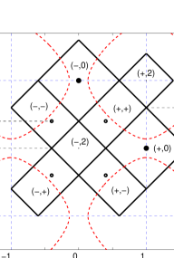
Figure 1: Partition of non-equivalent momenta into eight disjoint regions (rectangles), whose union under suitable translations by reciprocal lattice vectors is the first Brillouin zone. The regions are labelled by pairs of indices $(r,s)$ with $s=0$ corresponding to antinodal fermions, $s=\pm$ nodal fermions, and $s=2$ in- or out fermions. The dashed curves is a superimposed non-interacting Fermi surface corresponding to $t=1$, $t^{\prime}=-0.2$ and $\mu=-0.51(1)$. We set the lattice constant $a=1$.

The eight regions correspond to three classes of fermion degrees of freedom. We let $s=0$ label so-called antinodal fermions and define ${\bf K}_{+,0}\stackrel{{\scriptstyle\mbox{{\tiny def}}}}{{=}}(\pi/a,0)$ and ${\bf K}_{-,0}\stackrel{{\scriptstyle\mbox{{\tiny def}}}}{{=}}(0,\pi/a)$. Similarly, we let $s=\pm$ label so-called nodal fermions and define ${\bf K}_{r,s}=(rQ/a,rsQ/a)$ with a parameter $Q$ close, but not equal, to $\pi/2$. To get a simple geometry, it is useful to also introduce so-called in- and out fermions labelled by $s=2$. The corresponding points are ${\bf K}_{-,2}=(0,0)$ (in) and ${\bf K}_{+,2}=(\pi/a,\pi/a)$ (out), i.e. the center and corners of the Brillouin zone. In the following, one can equally well think of the in- and out fermions as belonging to the nodal fermions. We also define new fermion operators $\hat{c}_{r,s,\alpha}^{({\dagger})}({\bf k})=\hat{c}_{\alpha}^{({\dagger})}({\bf K}_{r,s}+{\bf k})$ such that the Hubbard Hamiltonian in (13) can be represented as

$$H_{{\text{Hubb}}}^{\phantom{{\dagger}}}=H_{{\text{Hubb}}}^{(0)}+H_{{\text{Hubb}}}^{(1)}$$ (16)

with

$$H_{{\text{Hubb}}}^{(0)}=\sum\limits_{\alpha=\uparrow,\downarrow}\sum\limits_{r=\pm}\sum\limits_{s=0,\pm,2}\sum\limits_{{\bf k}\in\Lambda^{*}_{r,s}}\left(\epsilon({\bf K}_{r,s}+{\bf k})-\mu+U/2\right)\hat{c}_{r,s,\alpha}^{{\dagger}}({\bf k})\hat{c}_{r,s,\alpha}^{\phantom{{\dagger}}}({\bf k})$$ (17)

the free part, and

$$\begin{split}H_{{\text{Hubb}}}^{(1)}=U\left(\frac{a}{L}\right)^{2}\sum\limits_{r_{j},s_{j}}\sum\limits_{{\bf k}_{j}\in\Lambda^{*}_{r_{j},s_{j}}}\sum_{{\bf n}\in{\mathbb{Z}}^{2}}\delta_{{\bf K}_{r_{1},s_{1}}-{\bf K}_{r_{2},s_{2}}+{\bf K}_{r_{3},s_{3}}-{\bf K}_{r_{4},s_{4}}+{\bf k}_{1}-{\bf k}_{2}+{\bf k}_{3}-{\bf k}_{4},2\pi{\bf n}/a}\\ \times\hat{c}_{r_{1},s_{1},\uparrow}^{\dagger}({\bf k}_{1})\hat{c}_{r_{2},s_{2},\uparrow}^{\phantom{{\dagger}}}({\bf k}_{2})\hat{c}_{r_{3},s_{3},\downarrow}^{\dagger}({\bf k}_{3})\hat{c}_{r_{4},s_{4},\downarrow}^{\phantom{{\dagger}}}({\bf k}_{4})\end{split}$$ (18)

the interaction part.

We will assume that there exists some underlying Fermi surface dominating the low-energy physics of the interacting model near half-filling, and that this surface has “flat parts” that can be approximated by a straight line segment or Fermi arc in each nodal region. Furthermore, we assume that the parameter $Q$ is such that each ${\bf K}_{r,s=\pm}$ lies on this underlying Fermi surface ($Q$ is the analogue of $k_{F}$ in the corresponding 1D model). We make no assumption on the geometry of the Fermi surface in the antinodal regions.

In the following, we concentrate on that part of (17)–(18) that only involves the nodal fermions ($s=\pm$); the end-result for the effective nodal Hamiltonian is given in the next secion, while the inclusion of antinodal fermions is discussed in Section 5. In Appendix B, the approximations introduced below (except for the continuum limit) are also applied to the antinodal (and in- and out) fermions in order to highlight similarities and differences between the fermions. In the appendices, we also include a nn interaction in the lattice Hamiltonian.

We expand the tight-binding band relations $\epsilon({\bf K}_{r,s}+{\bf k})$ for the nodal fermions as

$$\epsilon({\bf K}_{r,s}+{\bf k})=\epsilon({\bf K}_{r,s})+\varepsilon_{r,s}({\bf k})+O(|a{\bf k}|^{2}),\qquad r,s=\pm$$ (19)

with

$$\varepsilon_{r,s}({\bf k})=v_{F}rk_{s},\qquad v_{F}=2\sqrt{2}\sin(Q)\left[t+2t^{\prime}\cos(Q)\right]a$$ (20)

and where we use coordinates $k_{\pm}=(k_{1}\pm k_{2})/\sqrt{2}$. Our first approximation is to only keep terms up to linear order in $|a{\bf k}|$.

The interaction in the Hubbard Hamiltonian consists of those scattering processes $({\bf k}_{2},{\bf k}_{4})\to({\bf k}_{1},{\bf k}_{3})$ that conserve overall momenta (up to reciprocal lattice vectors). When writing the Hubbard Hamiltonian in terms of the operators $\hat{c}^{({\dagger})}_{r,s,\alpha}({\bf k})$, conservation of momenta corresponds to the following requirement

$$({\bf K}_{r_{1},s_{1}}+{\bf k}_{1})-({\bf K}_{r_{2},s_{2}}+{\bf k}_{2})+({\bf K}_{r_{3},s_{3}}+{\bf k}_{3})-({\bf K}_{r_{4},s_{4}}+{\bf k}_{4})\in(2\pi/a){\mathbb{Z}}^{2}$$ (21)

with ${\bf k}_{j}\in\Lambda_{r_{j},s_{j}}^{*}$. The next approximation is to reduce the number of (nodal) interaction terms in the Hubbard Hamiltonian by imposing the additional constraint

$${\bf K}_{r_{1},s_{1}}-{\bf K}_{r_{2},s_{2}}+{\bf K}_{r_{3},s_{3}}-{\bf K}_{r_{4},s_{4}}\in(2\pi/a){\mathbb{Z}}^{2}$$ (22)

for interaction terms that we keep. If all momenta lie strictly on a Fermi arc, the constraint (22) follows from momentum conservation. All possible combinations of $(r_{j},s_{j})$ satisfying this constraint when $Q\neq\pi/2$ are given in Table 1 in Appendix B. If $Q=\pi/2$ there are additional (and potentially gap-inducing) umklapp processes; it is tempting to identify this value with the half-filled model.

Obvious solutions to the constraint in (22) is to set either $(r_{1},s_{1})=(r_{2},s_{2})$ and $(r_{3},s_{3})=(r_{4},s_{4})$, or $(r_{1},s_{1})=(r_{4},s_{4})$ and $(r_{2},s_{2})=(r_{3},s_{3})$. These combinations naturally lead to the definition of density- and spin operators $\hat{\rho}_{r,s}^{\phantom{{\dagger}}}$ and $\hat{S}_{r,s}^{i}$, $i=1,2,3$, corresponding to each pair of flavor indices. For example, the nodal density operators are

$$\hat{\rho}_{r,s}({\bf p})=\sum\limits_{\alpha=\uparrow,\downarrow}\sum\limits_{{\bf k}_{1},{\bf k}_{2}\in\Lambda^{*}_{r,s}}\hat{c}^{\dagger}_{r,s,\alpha}({\bf k}_{1})\hat{c}^{\phantom{{\dagger}}}_{r,s,\alpha}({\bf k}_{2})\delta_{{\bf k}_{1}+{\bf p},{\bf k}_{2}}.$$ (23)

The interaction terms in the truncated Hubbard Hamiltonian with the above combinations for $(r_{j},s_{j})$ are products of these bilinears, i.e. $\hat{\rho}_{r,s}\hat{\rho}_{r^{\prime},s^{\prime}}$ and $\hat{\bf S}_{r,s}\cdot\hat{\bf S}_{r^{\prime},s^{\prime}}$. The constraint in (22) also allows for interaction terms involving pairing bilinears of the form $\hat{\psi}^{({\dagger})}\hat{\psi}^{({\dagger})}$. We define associated pairing operators denoted by $\hat{P}_{r,s}^{\mu}$, $\mu=0,1,2,3$, and write these interaction terms as $\hat{P}_{r,s}^{\dagger}\cdot\hat{P}_{r^{\prime},s^{\prime}}^{\phantom{{\dagger}}}$ with $\hat{P}_{r,s}^{\phantom{{\dagger}}}=(\hat{P}^{0}_{r,s},\hat{P}^{1}_{r,s},\hat{P}^{2}_{r,s},\hat{P}^{3}_{r,s})$.

The components of the momenta in the nodal sets $\Lambda_{r,s=\pm}^{*}$ are restricted by cutoffs proportional to the inverse lattice constant. Our partial contnuum limit for the nodal fermions involves removing the cutoff in the directions orthogonal to each Fermi arc. To this end, we normal-order the kinetic part and the bilinears in the truncated interaction with respect to a state $\Omega$ (the Dirac sea) in which all momenta up to the Fermi arcs in the nodal regions are occupied.

Consider now region $(+,+)$ in Figure 1. After removing the cutoff in the $k_{+}$-direction, it would be possible to bosonize the nodal fermions by treating the $k_{+}$ as an unbounded 1D chain of momenta and $k_{-}$ a flavor index labelling each chain. However, as discussed in the introduction, this does not lead to simple bosonic commutation relations for (23); only densities with momentum exchange in the $k_{+}$-direction would behave as bosons and one cannot treat momentum exchange between fermions on different chains. Instead, it is more fruitful to first do a Fourier transformation (change of basis) in the $k_{-}$-direction and then bosonize the fermions using a new flavor index $x_{-}$ [44, 56]. If one also removes the cutoff in the $k_{-}$-direction, the commutation relations of the (normal-ordered and rescaled) densities in (23) become that of 2D bosons. However, this limit is delicate as the (normal-ordered) Hamiltonian would then no longer be bounded from below; see the next section.

A mathematically more sound way to proceed is to keep the cutoff and instead modify the nodal density operators in (23); we define the normal-ordered density operators

$$\hat{J}_{r,s=\pm}^{0}({\bf p})=\sum\limits_{\alpha}\sum\limits_{{\bf k}_{1},{\bf k}_{2}\in\Lambda^{*}_{s}}:\!\hat{c}^{\dagger}_{r,s,\alpha}({\bf k}_{1})\hat{c}^{\phantom{{\dagger}}}_{r,s,\alpha}({\bf k}_{2})\!:\sum\limits_{n\in{\mathbb{Z}}}\delta_{{\bf k}_{1}+{\bf p}+2\pi n{\bf e}_{-s}/\tilde{a},{\bf k}_{2}}$$ (24)

with ${\bf e}_{-s}$ a unit vector in the direction of the Fermi arc. Here $\tilde{a}=\sqrt{2}a/({1-\kappa})$ with the length of each Fermi arc given by $2\pi/\tilde{a}$. This operator is obtained from (23) by adding “umklapp terms” corresponding to $n\neq 0$. As shown in [58], it is possible to send $\tilde{a}\to 0^{+}$ on the level of correlation functions. We do a similar regularization for the spin operators. With this, one obtains our effective nodal Hamiltonian; see Equation (LABEL:Regularised_nodal_Hamiltonian) in the next section.

4 Nodal fermions

We formulate the nodal part of the effective QFT model obtained from our partial continuum limit of the 2D Hubbard model near half-filling. We also show that the nodal fermions can be bosonized using exact methods. Some of these results are straightforward generalisations of the corresponding ones obtained for the so-called Mattis model in [58], and in those instances we will be rather brief in the presentation. Further mathematical details are also given in Appendix C. In this section, the flavor indices are always $r,s=\pm$.

4.1 The nodal Hamiltonian

We rescale the nodal fermion operators by setting $\hat{\psi}_{r,s,\alpha}({\bf k})=L/(2\pi)\hat{c}_{r,s,\alpha}({\bf k})$ such that

$$\{\hat{\psi}^{\phantom{{\dagger}}}_{r,s,\alpha}({\bf k}),\hat{\psi}^{{\dagger}}_{r^{\prime},s^{\prime},\alpha^{\prime}}({\bf k}^{\prime})\}=[L/(2\pi)]^{2}\delta_{r,r^{\prime}}\delta_{s,s^{\prime}}\delta_{\alpha,\alpha^{\prime}}\delta_{{\bf k},{\bf k}^{\prime}},\quad\{\hat{\psi}^{\phantom{{\dagger}}}_{r,s,\alpha}({\bf k}),\hat{\psi}^{\phantom{{\dagger}}}_{r^{\prime},s^{\prime},\alpha^{\prime}}({\bf k}^{\prime})\}=0.$$ (25)

The momenta ${\bf k}$ are in the (unbounded) sets

$$\Lambda_{s}^{*}=\left\{{\bf k}\in\frac{2\pi}{L}\Bigl{(}\mathbb{Z}+\frac{1}{2}\Bigr{)}^{2}\;:\;-\frac{\pi}{\tilde{a}}\leq k_{-s}<\frac{\pi}{\tilde{a}}\right\}.$$ (26)

The nodal part of the effective model is obtained from a Dirac vacuum $\Omega$ satisfying

$$\hat{\psi}^{\phantom{{\dagger}}}_{r,s,\alpha}({\bf k})\Omega=\hat{\psi}^{\dagger}_{r,s,\alpha}(-{\bf k})\Omega=0,\quad\mbox{for all }{\bf k}\in\Lambda_{s}^{*}\;\mbox{ such that }\;rk_{s}>0$$ (27)

with $\langle\Omega,\Omega\rangle=1$. The specific choice of filling for the antinodal fermion states in $\Omega$ is unimportant; we assume for simplicity that no state is occupied. We also introduce ordinary fermion normal-ordering with respect to $\Omega$ such that $:\!\mathcal{O}\!:\,=\mathcal{O}-\langle\Omega,\mathcal{O}\Omega\rangle$ for fermion bilinears $\mathcal{O}=\hat{\psi}^{\dagger}_{r,s,\alpha}({\bf k})\hat{\psi}^{\phantom{{\dagger}}}_{r^{\prime},s^{\prime},\alpha^{\prime}}({\bf k}^{\prime})$.

We define the following nodal bilinear operators

$$\hat{J}_{r,s}^{\mu}({\bf p}) =\sum\limits_{\alpha,\beta}\sum\limits_{{\bf k}_{1},{\bf k}_{2}\in\Lambda^{*}_{s}}\sum\limits_{n\in{\mathbb{Z}}}\Bigl{(}\frac{2\pi}{L}\Bigr{)}^{2}:\!\hat{\psi}^{\dagger}_{r,s,\alpha}({\bf k}_{1})\sigma_{\alpha,\beta}^{\mu}\hat{\psi}^{\phantom{{\dagger}}}_{r,s,\beta}({\bf k}_{2})\!:\delta_{{\bf k}_{1}+{\bf p},{\bf k}_{2}+2\pi n{\bf e}_{-s}/\tilde{a}}$$ (28)

$$\hat{P}_{r,s}^{\mu}({\bf p}) =\frac{1}{2}\sum\limits_{\alpha,\beta}\sum\limits_{{\bf k}_{1},{\bf k}_{2}\in\Lambda^{*}_{r,s}}\Bigl{(}\frac{2\pi}{L}\Bigr{)}^{2}\hat{\psi}^{\phantom{{\dagger}}}_{-r,s,\alpha}({\bf k}_{1})\sigma_{\alpha,\beta}^{\mu}\hat{\psi}^{\phantom{{\dagger}}}_{r,s,\beta}({\bf k}_{2})\delta_{{\bf k}_{1}+{\bf k}_{2},{\bf p}}$$ (29)

with $r,s=\pm$ and $\mu=0,1,2,3$; here $\sigma^{i}$, $i=1,2,3$, are the Pauli matrices, $\sigma_{\alpha,\beta}^{0}=\delta_{\alpha,\beta}$ and the momenta ${\bf p}$ are in the set

$$\tilde{\Lambda}_{s}^{*}=\left\{{\bf p}=(p_{+},p_{-})\in(2\pi/L){\mathbb{Z}}\texttwosuperior\;:\;-{\pi}/{\tilde{a}}\leq p_{-s}<{\pi}/{\tilde{a}}\right\}.$$ (30)

Spin operators are given by the simple rescaling $\hat{S}_{r,s}^{i}=\hat{J}_{r,s}^{i}/2$. We note that removing the cutoff in the summation of momenta ${\bf k}_{1},{\bf k}_{2}$ in (29) would lead to ill-defined operators [39]. For example, acting with such operators on $\Omega$ would result in a state of infinite norm.

The nodal part of the effective Hamiltonian is now defined as

$$\begin{split}&H_{n}=H+U\sum\limits_{r,r^{\prime},s=\pm}\sum\limits_{{\bf p}}\Bigl{(}\frac{a}{L}\Bigr{)}^{2}\chi({\bf p})\hat{P}_{r,s}^{\dagger}({\bf p})\cdot\hat{P}_{r^{\prime},-s}^{\phantom{{\dagger}}}({\bf p})\\ &H=H_{0}+H_{1}\end{split}$$ (31)

with

$$H_{0}=v_{F}\sum\limits_{\alpha=\pm}\sum\limits_{r,s=\pm}\sum\limits_{{\bf k}\in\Lambda_{s}^{*}}\Bigl{(}{\frac{{2\pi}}{L}}\Bigr{)}^{2}rk_{s}:\hat{\psi}_{r,s,\alpha}^{\dagger}({\bf k})\hat{\psi}_{r,s,\alpha}^{\phantom{{\dagger}}}({\bf k}):$$ (32)

the free part, and

$$\begin{split}H_{1}=\frac{U}{2}\sum\limits_{{\bf p}}\Bigl{(}\frac{a}{L}\Bigr{)}^{2}\chi({\bf p})\Bigl{(}\sum\limits_{s=\pm}\bigl{(}\sum\limits_{r=\pm}\hat{J}_{r,s}^{0{\dagger}}\hat{J}_{r,s}^{0}+\hat{J}_{+,s}^{0{\dagger}}\hat{J}_{-,s}^{0}-{\hat{\bf J}}_{+,s}^{\dagger}\cdot{\hat{\bf J}}_{-,s}^{\phantom{{\dagger}}}\bigr{)}\\ +\sum\limits_{r,r^{\prime}=\pm}\bigl{(}\hat{J}_{r,+}^{0{\dagger}}\hat{J}_{r^{\prime},-}^{0}-{\hat{\bf J}}_{r,+}^{\dagger}\cdot{\hat{\bf J}}_{r^{\prime},-}^{\phantom{{\dagger}}}\bigr{)}\Bigr{)}\end{split}$$ (33)

the density- and spin interaction part; here ${\hat{\bf J}}_{r,s}=(\hat{J}_{r,s}^{1},\hat{J}_{r,s}^{2},\hat{J}_{r,s}^{3})$ and we suppress common arguments of ${\bf p}$. Furthermore, we have introduced a cutoff function for possible momentum exchange in the interaction by

$$\chi({\bf p})=\begin{cases}1&\text{if }-{\pi}/{\tilde{a}}\leq p_{\pm}<{\pi}/{\tilde{a}}\\ 0&\text{otherwise}\end{cases}.$$ (34)

The nodal Hamiltonian in (LABEL:Regularised_nodal_Hamiltonian) contains different types of scattering processes. Terms involving the bilinears in (28) correspond to processes for which both fermions remain near the same Fermi arc, and for which their spin projection may or may not be reversed. In contrast, terms involving (29) are such that both fermions are scattered from one Fermi arc to another. As we will see below, these latter terms cannot be easily analyzed using our methods.

We also summarize our conventions for Fourier transforms of nodal operators (similar expressions can be found in [58]). Define nodal fermion field operators by

$$\psi_{r,s,\alpha}^{\phantom{{\dagger}}}({\bf x})=\frac{1}{2\pi}\sum_{{\bf k}\in\Lambda^{*}_{s}}\Bigl{(}\frac{2\pi}{L}\Bigr{)}^{2}\hat{\psi}_{r,s,\alpha}({\bf k})\,{\rm e}^{{\rm i}{\bf k}\cdot{\bf x}}\qquad(s=\pm),$$ (35)

with “positions” ${\bf x}$ in

$$\Lambda_{s}=\left\{{\bf x}\in{\mathbb{R}}^{2}\,:\,x_{s}\in\mathbb{R},\;x_{-s}\in\tilde{a}\mathbb{Z},\;-{L}/{2}\leq x_{\pm}<{L}/{2}\right\}$$ (36)

and which obey the anticommutation relations

$$\{\psi^{\phantom{{\dagger}}}_{r,s,\sigma}({\bf x}),\psi^{{\dagger}}_{r^{\prime},s^{\prime},\sigma^{\prime}}({\bf y})\}=\delta_{r,r^{\prime}}^{\phantom{{\dagger}}}\delta_{s,s^{\prime}}^{\phantom{{\dagger}}}\delta_{\sigma,\sigma^{\prime}}^{\phantom{{\dagger}}}\tilde{\delta}_{s}^{\phantom{{\dagger}}}({\bf x}-{\bf y}),\qquad\tilde{\delta}_{s}({\bf x})=\delta(x_{s})\frac{1}{\tilde{a}}\delta_{x_{-s},0}.$$ (37)

The (regularized) Fourier transforms of the nodal density- and spin operators in (28) are defined as

$$\begin{split}J_{r,s}^{\mu}({\bf x};\epsilon)=\sum_{{\bf p}\in\tilde{\Lambda}^{*}_{s}}\frac{1}{L^{2}}\hat{J}_{r,s}^{\mu}({\bf p})\,{\rm e}^{{\rm i}{\bf p}\cdot{\bf x}-\epsilon|p_{s}|/2},\qquad J_{r,s}^{\mu}({\bf x})=\lim_{\epsilon\to 0^{+}}J_{r,s}^{\mu}({\bf x};\epsilon)\end{split}$$ (38)

with $\epsilon>0$ infinitesimal. Using these operators, it is for example possible to rewrite $H_{0}$ in (32) in “position” space and thus obtain a well-defined regularised expression replacing the free part of (2)

$$H_{0}=v_{F}\sum\limits_{\alpha=\pm}\sum\limits_{r,s=\pm}\;\,\tilde{\!\!\!\int\limits_{{s}}}\mathrm{d}^{2}x\,:\!\psi^{\dagger}_{r,s,\alpha}({\bf x})(-{\rm i}r\partial_{s})\psi_{r,s,\alpha}^{\phantom{{\dagger}}}({\bf x})\!:$$ (39)

where we have defined

$$\;\,\tilde{\!\!\!\int\limits_{{s}}}\mathrm{d}^{2}x\,=\int\limits_{-L/2}^{L/2}\mathrm{d}x_{s}\sum_{x_{-s}\in\Lambda_{1\rm D}}\tilde{a}$$ (40)

and

$$\Lambda_{1\rm D}=\left\{x\in\tilde{a}\mathbb{Z}\;:\;-{L}/{2}\leq x<{L}/{2}\right\}.$$ (41)

The free part of the nodal Hamiltonian (39) can thus be interpreted as a system of 1D (massless) Dirac fermions where, for each $s=\pm$, $x_{s}\in\bigl{[}-L/2,L/2\bigr{)}$ is a (continuous) spatial variable and $x_{-s}\in\Lambda_{1D}$ a (discrete) flavor index. Analogous regularized expressions may be written down for the interaction part of (2). Likewise, insertion of the inverse relation to (35) into (38), using (28), yields (3).

4.2 Bosonization

The presence of the Dirac vacuum satisfying (27) leads to anomalous commutator relations [27] for the fermion bilinears in (28) (see Appendix C for proof)

$$\begin{split}\left[\hat{J}_{r,s}^{0}({\bf p}),\hat{J}_{r,s}^{0}({\bf p}^{\prime})\right]&=r\frac{4\pi p_{s}}{\tilde{a}}\Bigl{(}\frac{L}{2\pi}\Bigr{)}^{2}\delta_{{\bf p}+{\bf p}^{\prime},{\bf 0}}\\ \left[\hat{J}_{r,s}^{i}({\bf p}),\hat{J}_{r,s}^{j}({\bf p}^{\prime})\right]&=2{\rm i}\sum\limits_{k=1}^{3}\epsilon_{ijk}\hat{J}_{r,s}^{k}({\bf p}+{\bf p}^{\prime})+r\frac{4\pi p_{s}}{\tilde{a}}\Bigl{(}\frac{L}{2\pi}\Bigr{)}^{2}\delta_{{\bf p}+{\bf p}^{\prime},{\bf 0}}\delta_{i,j}\end{split}$$ (42)

with all other commutators vanishing; $\epsilon_{ijk}$ is the totally antisymmetric tensor and $\epsilon_{123}=1$. Furthermore, $\hat{J}_{r,s}^{\mu}({\bf p})\Omega=0$ for all ${\bf p}$ such that $rp_{s}\geq 0$. Using (42) together with (38), one obtains the commutation relations in (4) (everywhere replacing $\delta({\bf x})$ with $\tilde{\delta}_{s}({\bf x})$ defined in (37)).

We introduce spin-dependent densities,

$$\hat{J}_{r,s,\uparrow}({\bf p})=\bigl{(}\hat{J}_{r,s}^{0}({\bf p})+\hat{J}_{r,s}^{3}({\bf p})\bigr{)}/2,\qquad\hat{J}_{r,s,\downarrow}({\bf p})=\bigl{(}\hat{J}_{r,s}^{0}({\bf p})-\hat{J}_{r,s}^{3}({\bf p})\bigr{)}/2,$$ (43)

which by (42) satisfy the commutation relations

$$\Bigl{[}\hat{J}_{r,s,\alpha}({\bf p}),\hat{J}_{r,s,\alpha^{\prime}}({\bf p}^{\prime})\Bigr{]}=r\delta_{\alpha,\alpha^{\prime}}\frac{2\pi p_{s}}{\tilde{a}}\Bigl{(}\frac{L}{2\pi}\Bigr{)}^{2}\delta_{{\bf p}+{\bf p}^{\prime},{\bf 0}}.$$ (44)

It follows that the rescaled densities

$$b_{s,\alpha}({\bf p})=\begin{cases}-\frac{{\rm i}}{L}\sqrt{\frac{2\pi\tilde{a}}{|p_{s}|}}\hat{J}_{+,s,\alpha}({\bf p})&\text{if $p_{s}>0$}\\ \phantom{-}\frac{{\rm i}}{L}\sqrt{\frac{2\pi\tilde{a}}{|p_{s}|}}\hat{J}_{-,s,\alpha}({\bf p})&\text{if $p_{s}<0$}\end{cases}$$ (45)

obey the defining relations of 2D boson creation- and annihilation operators,

$$[b^{\phantom{{\dagger}}}_{s,\alpha}({\bf p}),b^{\dagger}_{s^{\prime},\alpha^{\prime}}({\bf p}^{\prime})]=\delta_{s,s^{\prime}}\delta_{\alpha,\alpha^{\prime}}\delta_{{\bf p},{\bf p}^{\prime}},\qquad[b^{\phantom{{\dagger}}}_{s,\alpha}({\bf p}),b^{\phantom{{\dagger}}}_{s^{\prime},\alpha^{\prime}}({\bf p}^{\prime})]=0,\qquad b^{\phantom{{\dagger}}}_{s,\alpha}({\bf p})\Omega=0.$$ (46)

The boson operators in (45) are defined for momenta ${\bf p}\in\tilde{\Lambda}_{s}^{*}$ such that $p_{s}\neq 0$; we denote this set as $\hat{\Lambda}_{s}^{*}$ (see (89)). Corresponding to momenta with $p_{s}=0$, we also introduce so-called zero mode operators, or simply zero modes, $N_{r,s,\alpha}(x)$ with $x\in\Lambda_{1\rm D}$ (see (41)); their definition is given in Appendix C. To complete the bosonization of the nodal fermions, we also need the so-called Klein factors $R_{r,s,\alpha}(x)$ conjugate to the zero modes. These are sometimes called charge shift- or ladder operators [60] as they raise or lower the number of fermions (with flavor indices $(r,s,\alpha,x)$) by one when acting on the Dirac vacuum. The Klein factors, together with the boson operators introduced above, span the nodal part of the fermion Fock space when acting on the Dirac vacuum; see Appendix C for details. This enables us to express nodal operators in terms of Klein factors and density operators; in particular, the fermion field operator in (35) has the form

$$\begin{split}\psi_{r,s,\alpha}^{\phantom{{\dagger}}}({\bf x})\sim\frac{1}{\sqrt{2\pi\tilde{a}\epsilon}}R_{r,s,\alpha}(x_{-s})^{-r}\exp\Bigl{(}r\frac{\tilde{a}}{2\pi}\sum_{{\bf p}\in\hat{\Lambda}_{s}}\Bigl{(}\frac{2\pi}{L}\Bigr{)}^{2}\frac{1}{p_{s}}\hat{J}_{r,s,\alpha}({\bf p})\,{\rm e}^{{\rm i}{\bf p}\cdot{\bf x}}\,{\rm e}^{-\epsilon|p_{s}|/2}\Bigr{)}\end{split}$$ (47)

with $\epsilon\to 0^{+}$ implicit; precise statements are given in Appendix C.

We define boson normal-ordering with respect to the Dirac vacuum $\Omega$ such that

$$\stackrel{{\scriptstyle\scriptscriptstyle\times}}{{\scriptscriptstyle\times}}\!\hat{J}_{r,s}^{\mu}({\bf p})\hat{J}_{r^{\prime},s^{\prime}}^{\mu}({\bf p}^{\prime})\!\stackrel{{\scriptstyle\scriptscriptstyle\times}}{{\scriptscriptstyle\times}}\,\stackrel{{\scriptstyle\mbox{{\tiny def}}}}{{=}}\begin{cases}\hat{J}_{r,s}^{\mu}({\bf p})\hat{J}_{r^{\prime},s^{\prime}}^{\mu}({\bf p}^{\prime})&\text{if $rp_{s}<0$}\\ \hat{J}_{r^{\prime},s^{\prime}}^{\mu}({\bf p}^{\prime})\hat{J}_{r,s}^{\mu}({\bf p})&\text{if $rp_{s}\geq 0$}\end{cases}\qquad(\mu=0,1,2,3)$$ (48)

(analogous expressions hold for $\hat{J}_{r,s,\alpha}$). Then the following operator identities hold true

$$\begin{split}\sum\limits_{\alpha=\uparrow,\downarrow}\sum\limits_{{\bf k}\in\Lambda_{s}^{*}}\Bigl{(}{\frac{{2\pi}}{L}}\Bigr{)}^{2}rk_{s}:\!\hat{\psi}_{r,s,\alpha}^{\dagger}\hat{\psi}_{r,s,\alpha}^{\phantom{{\dagger}}}\!:&=\tilde{a}\pi\sum\limits_{\alpha=\uparrow,\downarrow}\sum_{{\bf p}\in\tilde{\Lambda}_{s}^{*}}\frac{1}{L^{2}}\stackrel{{\scriptstyle\scriptscriptstyle\times}}{{\scriptscriptstyle\times}}\!\hat{J}_{r,s,\alpha}^{\dagger}\hat{J}_{r,s,\alpha}^{\phantom{{\dagger}}}\!\stackrel{{\scriptstyle\scriptscriptstyle\times}}{{\scriptscriptstyle\times}}\\ &=\frac{\tilde{a}\pi}{2}\sum\limits_{{\bf p}\in\tilde{\Lambda}_{s}^{*}}\frac{1}{L^{2}}\stackrel{{\scriptstyle\scriptscriptstyle\times}}{{\scriptscriptstyle\times}}\!\Bigl{(}\hat{J}_{r,s}^{0{\dagger}}\hat{J}_{r,s}^{0}+\frac{1}{3}{\hat{\bf J}}_{r,s}^{\dagger}\cdot{\hat{\bf J}}_{r,s}^{\phantom{{\dagger}}}\Bigr{)}\!\stackrel{{\scriptstyle\scriptscriptstyle\times}}{{\scriptscriptstyle\times}}\end{split}$$ (49)

with the momentum sets defined in (26) and (30). The first identity is an application of the Kronig identity, while the second is a Sugawara construction; see Appendix C.

4.3 An exactly solvable model of 2D electrons

We discuss the bosonization of the nodal Hamiltonian in (LABEL:Regularised_nodal_Hamiltonian) using the results obtained above. Inserting the last expression of (49) into (32) gives (5) with (cf. (6))

$$\begin{split}H_{C}^{\phantom{{\dagger}}}=\frac{v_{F}\pi\tilde{a}}{2}\sum\limits_{{\bf p}}\frac{1}{L^{2}}\stackrel{{\scriptstyle\scriptscriptstyle\times}}{{\scriptscriptstyle\times}}\!\Big{(}\sum\limits_{r,s=\pm}\left(\left(1+2\gamma\chi({\bf p})\right)\hat{J}_{r,s}^{0{\dagger}}{\hat{J}}_{r,s}^{0}+\gamma\chi({\bf p})\hat{J}_{r,s}^{0{\dagger}}{\hat{J}}_{-r,s}^{0}\right)\\ +2\gamma\chi({\bf p})\sum\limits_{r,r^{\prime}=\pm}\hat{J}_{r,+}^{0{\dagger}}{\hat{J}}_{r^{\prime},-}^{0}\Bigr{)}\!\stackrel{{\scriptstyle\scriptscriptstyle\times}}{{\scriptscriptstyle\times}}\end{split}$$ (50)

$$\begin{split}H_{\bf{S}}^{\phantom{{\dagger}}}=\frac{v_{F}\pi\tilde{a}}{2}\sum\limits_{{\bf p}}\frac{1}{L^{2}}\stackrel{{\scriptstyle\scriptscriptstyle\times}}{{\scriptscriptstyle\times}}\!\Big{(}\sum\limits_{r,s=\pm}\left(\hat{\bf J}_{r,s}^{\dagger}\cdot{\hat{\bf J}}_{r,s}^{\phantom{{\dagger}}}/3-\gamma{\chi}({\bf p})\hat{\bf J}_{r,s}^{\dagger}\cdot{\hat{\bf J}}_{-r,s}^{\phantom{{\dagger}}}\right)\\ -2\gamma{\chi}({\bf p})\sum\limits_{r,r^{\prime}=\pm}\hat{\bf J}_{r,+}^{\dagger}\cdot{\hat{\bf J}}_{r^{\prime},-}^{\phantom{{\dagger}}}\Bigr{)}\!\stackrel{{\scriptstyle\scriptscriptstyle\times}}{{\scriptscriptstyle\times}}\end{split}$$ (51)

and with the dimensionsless coupling constant

$$\gamma=\frac{a^{2}U}{2\pi\tilde{a}v_{F}}.$$ (52)

We emphasize that this does not imply (exact) spin-charge separation of the nodal Hamiltonian; there is also the second term on the right hand side of (LABEL:Regularised_nodal_Hamiltonian) that does not have a simple bosonized form (although it can indeed be expressed in terms of Klein factors, density- and spin operators using Proposition C.3 in Appendix C).

A complete analysis of (50)–(51) will not be attempted in the present paper. Instead, we will focus in the remainder of this section on the “abelian” part of $H$ obtained by breaking manifest spin rotation invariance, and which we denote by $H_{M}$ due to its similarity to the so-called Mattis Hamiltonian in [58]. More specifically, we write

$$\begin{split}H=H_{M}-\frac{U}{4}\sum\limits_{{\bf p}}\Bigl{(}\frac{a}{L}\Bigr{)}^{2}\chi({\bf p})\Bigl{(}&\sum\limits_{s=\pm}\bigl{(}\hat{J}_{+,s}^{+}(-{\bf p})\hat{J}_{-,s}^{-}({\bf p})+h.c.\bigr{)}\\ &+\sum\limits_{r,r^{\prime}=\pm}\bigl{(}\hat{J}_{r,+}^{+}(-{\bf p})\hat{J}_{r^{\prime},-}^{-}({\bf p})+h.c.\bigr{)}\Bigr{)}\end{split}$$ (53)

with the raising- and lowering operators defined as usual, $\hat{J}_{r,s}^{\pm}=\bigl{(}\hat{J}_{r,s}^{1}\pm{\rm i}\hat{J}_{r,s}^{2}\bigr{)}/2$, and where $H_{M}$ only depends on $\hat{J}_{r,s}^{0}$ and $\hat{J}_{r,s}^{3}$. Using results from Section 4.2, it is possible to write the Hamiltonian $H_{M}$ in terms of free bosons. Define

$$\begin{aligned} \hat{\Phi}_{C;s}({\bf p})\stackrel{{\scriptstyle\mbox{{\tiny def}}}}{{=}}&\sqrt{\frac{\tilde{a}}{8\pi}}\frac{1}{{\rm i}p_{s}}\Bigl{(}\hat{J}_{+,s}^{0}({\bf p})+\hat{J}_{-,s}^{0}({\bf p})\Bigr{)},&\quad\hat{\Pi}_{C;s}({\bf p})\stackrel{{\scriptstyle\mbox{{\tiny def}}}}{{=}}&\sqrt{\frac{\tilde{a}}{8\pi}}\Bigl{(}-\hat{J}_{+,s}^{0}({\bf p})+\hat{J}_{-,s}^{0}({\bf p})\Bigr{)}\\ \hat{\Phi}_{{S};s}({\bf p})\stackrel{{\scriptstyle\mbox{{\tiny def}}}}{{=}}&\sqrt{\frac{\tilde{a}}{8\pi}}\frac{1}{{\rm i}p_{s}}\Bigl{(}\hat{J}_{+,s}^{3}({\bf p})+\hat{J}_{-,s}^{3}({\bf p})\Bigr{)},&\quad\hat{\Pi}_{{S};s}({\bf p})\stackrel{{\scriptstyle\mbox{{\tiny def}}}}{{=}}&\sqrt{\frac{\tilde{a}}{8\pi}}\Bigl{(}-\hat{J}_{+,s}^{3}({\bf p})+\hat{J}_{-,s}^{3}({\bf p})\Bigr{)}\end{aligned}$$ (54)

for $s=\pm$ and 2D momenta ${\bf p}\in\hat{\Lambda}_{s}^{*}$. It follows that these obey the defining relations of 2D neutral bosons, i.e.

$${[}\hat{\Phi}^{\phantom{{\dagger}}}_{X;s}({\bf p}),\hat{\Pi}^{\dagger}_{X^{\prime};s^{\prime}}({\bf p}^{\prime}){]}={\rm i}\delta_{X,X^{\prime}}\delta_{s,s^{\prime}}\Bigl{(}\frac{L}{2\pi}\Bigr{)}^{2}\delta_{{\bf p},{\bf p}^{\prime}}$$ (55)

(all other commutators vanishing) and

$$\hat{\Pi}^{\dagger}_{X;s}({\bf p})=\hat{\Pi}^{\phantom{{\dagger}}}_{X;s}(-{\bf p}),\qquad\hat{\Phi}^{\dagger}_{X;s}({\bf p})=\hat{\Phi}^{\phantom{{\dagger}}}_{X;s}(-{\bf p}),$$ (56)

where we have used the symbolic notation $X,X^{\prime}=C,{S}$. Furthermore, applying the first equality in (49) to (32), together with (54), allows us to write

$$H_{M}=H_{C}^{\phantom{{\dagger}}}+H_{S}^{\phantom{{\dagger}}}$$ (57)

with

$$\begin{split}H_{C}^{\phantom{{\dagger}}}=&\frac{v_{F}}{2}\sum_{s=\pm}\sum_{{\bf p}\in\hat{\Lambda}^{*}_{s}}\Bigl{(}\frac{2\pi}{L}\Bigr{)}^{2}\stackrel{{\scriptstyle\scriptscriptstyle\times}}{{\scriptscriptstyle\times}}\!\Bigl{(}\bigl{(}1+\gamma\chi({\bf p})\bigr{)}\hat{\Pi}^{\dagger}_{C;s}\hat{\Pi}^{\phantom{{\dagger}}}_{C;s}\\ &+\bigl{(}1+3\gamma\chi({\bf p})\bigr{)}p_{s}^{2}\hat{\Phi}^{\dagger}_{C;s}\hat{\Phi}^{\phantom{{\dagger}}}_{C;s}+2\gamma p_{+}p_{-}\chi({\bf p})\hat{\Phi}^{\dagger}_{C;s}\hat{\Phi}^{\phantom{{\dagger}}}_{C;-s}\Bigr{)}\!\stackrel{{\scriptstyle\scriptscriptstyle\times}}{{\scriptscriptstyle\times}}+z.m.\end{split}$$ (58)

$$\begin{split}H_{S}=&\frac{v_{F}}{2}\sum_{s=\pm}\sum_{{\bf p}\in\hat{\Lambda}^{*}_{s}}\Bigl{(}\frac{2\pi}{L}\Bigr{)}^{2}\stackrel{{\scriptstyle\scriptscriptstyle\times}}{{\scriptscriptstyle\times}}\!\Bigl{(}\bigl{(}1+\gamma\chi({\bf p})\bigr{)}\hat{\Pi}^{\dagger}_{{S};s}\hat{\Pi}^{\phantom{{\dagger}}}_{{S};s}\\ &+\bigl{(}1-\gamma\chi({\bf p})\bigr{)}p_{s}^{2}\hat{\Phi}^{\dagger}_{{S};s}\hat{\Phi}^{\phantom{{\dagger}}}_{{S};s}-2\gamma p_{+}p_{-}\chi({\bf p})\hat{\Phi}^{\dagger}_{{S};s}\hat{\Phi}^{\phantom{{\dagger}}}_{{S};-s}\Bigr{)}\!\stackrel{{\scriptstyle\scriptscriptstyle\times}}{{\scriptscriptstyle\times}}+z.m.\end{split}$$ (59)

with $z.m.$ denoting terms involving zero mode operators; a complete solution including the zero modes is given in Appendix C.3.

The charge- and spin parts of $H_{M}$ in (57) each have the same structure as the bosonized Hamiltonian of the so-called Mattis model of spinless fermions studied in [58] (compare Equation (3.3) in [58] with (58) and (59)). As for the Mattis Hamiltonian, the right hand side of (57) can be diagonalised by a Bogoliubov transformation into a sum of decoupled harmonic oscillators and zero mode terms. To this end, define

$$b_{C;s}({\bf p})=\bigl{(}b_{s,\uparrow}({\bf p})+b_{s,\downarrow}({\bf p})\bigr{)}/\sqrt{2},\qquad b_{{S};s}({\bf p})=\bigl{(}b_{s,\uparrow}({\bf p})-b_{s,\downarrow}({\bf p})\bigr{)}/\sqrt{2}.$$ (60)

The Hamiltonian in (57) can then be diagonalized by a unitary operator $\mathcal{U}$ as follows (see Theorem C.5 in Appendix C.3)

$$\mathcal{U}^{\dagger}H_{M}\mathcal{U}=\sum_{s=\pm}\sum_{{\bf p}\in\hat{\Lambda}_{s}^{*}}\left(\omega_{C;s}^{\phantom{{\dagger}}}({\bf p})b_{C;s}^{\dagger}({\bf p})b^{\phantom{{\dagger}}}_{C;s}({\bf p})+\omega_{{S};s}^{\phantom{{\dagger}}}({\bf p})b_{{S};s}^{\dagger}({\bf p})b^{\phantom{{\dagger}}}_{{S};s}({\bf p})\right)+\mathcal{E}^{(0)}+z.m.$$ (61)

with

$$\omega_{C;\pm}^{\phantom{{\dagger}}}({\bf p})=\begin{cases}\tilde{v}_{F}^{C}\sqrt{\frac{1}{2}\Bigl{(}|{\bf p}|^{2}\pm\sqrt{|{\bf p}|^{4}-A_{C}\bigl{(}2p_{+}p_{-}\bigr{)}^{2}}\;\Bigr{)}}&\mbox{ if }\;\gamma\chi({\bf p})p_{+}p_{-}\neq 0\\ v_{F}\sqrt{\bigl{(}1+2\gamma\chi({\bf p})\bigr{)}^{2}-\bigl{(}\gamma\chi({\bf p})\bigr{)}^{2}}|p_{\pm}|&\mbox{ if }\;\gamma\chi({\bf p})p_{+}p_{-}=0\end{cases}$$ (62)

$$A_{C}=1-\bigl{[}{2\gamma}/({1+3\gamma})\bigr{]}^{2},\qquad\tilde{v}_{F}^{C}=v_{F}\sqrt{\bigl{(}1+2\gamma\bigr{)}^{2}-\gamma^{2}}$$ (63)

and

$$\omega_{{S};\pm}^{\phantom{{\dagger}}}({\bf p})=\begin{cases}\tilde{v}_{F}^{S}\sqrt{\frac{1}{2}\Bigl{(}|{\bf p}|^{2}\pm\sqrt{|{\bf p}|^{4}-A_{S}\bigl{(}2p_{+}p_{-}\bigr{)}^{2}}\;\Bigr{)}}&\mbox{ if }\;\gamma\chi({\bf p})p_{+}p_{-}\neq 0\\ v_{F}\sqrt{1-\bigl{(}\gamma\chi({\bf p})\bigr{)}^{2}}|p_{\pm}|&\mbox{ if }\;\gamma\chi({\bf p})p_{+}p_{-}=0\end{cases}$$ (64)

$$A_{S}=1-\bigl{[}2{\gamma}/({1-\gamma})\bigr{]}^{2},\qquad\tilde{v}_{F}^{S}=v_{F}\sqrt{1-\gamma^{2}}$$ (65)

the boson dispersion relations, and

$$\mathcal{E}^{(0)}=\frac{1}{2}\sum_{s=\pm}\sum_{{\bf p}\in\hat{\Lambda}_{s}^{*}}\bigl{(}\omega_{C;s}^{\phantom{{\dagger}}}({\bf p})+\omega_{{S};s}^{\phantom{{\dagger}}}({\bf p})-2v_{F}|p_{s}|\bigr{)}$$ (66)

the groundstate energy of $H_{M}$. This is well-defined if (12) is fulfilled. For the special case $t^{\prime}=0$, $\kappa=1/2$, and $Q\to\pi/2$, one obtains the upper bound $U/t<16\pi/3$.

In principle, one can now obtain the complete solution for the model defined by $H_{M}$ by stepwise generalizing the results given in [58] to the present case. For example, all correlation functions of nodal fermion operators in the thermal equilibrium state obtained from $H_{M}$ can be computed exactly by analytical methods. Furthermore, as shown in [58], zero modes do not contribute to correlation functions in the thermodynamic limit $L\to\infty$ (much like in 1D). The only exception are the Klein factors that need to be handled with some care; see Section 3.3 in [58].

5 Integrating out degrees of freedom

Up to now, we have studied the part that involves only nodal fermions in the effective Hamiltonian (7). Below, we will propose different ways of also including the antinodal fermions in the analysis.

5.1 Integrating out nodal fermions

The nodal- and antinodal fermions couple through various types of scattering processes in the Hubbard interaction (18) that we cannot treat in full generality. A simple approximation is to also introduce the constraint in (22) for nodal-antinodal processes. This leads to an effective interaction involving nodal- and antinodal bilinears of the same form as in (LABEL:Regularised_nodal_Hamiltonian); we refer to Appendix B for details. If we truncate this interaction further by only keeping terms involving the nodal bilinears $J^{0}_{r,s}$ and $J^{3}_{r,s}$, it is possible to integrate out the bosonized nodal fermions using a functional integral representation of the partition function. We set (cf. (153); note the abuse of notation for the left hand side)

$$H_{na}=\frac{U}{2}\sum\limits_{r,r^{\prime},s=\pm}\sum\limits_{{\bf p}}\Bigl{(}\frac{a}{L}\Bigr{)}^{2}\chi({\bf p})\Bigl{(}\hat{J}_{r,s}^{0}(-{\bf p})\hat{J}_{r^{\prime},0}^{0}({\bf p})-{\hat{J}}_{r,s}^{3}(-{\bf p}){\hat{J}}_{r^{\prime},0}^{3}({\bf p})\Bigr{)}$$ (67)

with the antinodal bilinears ($\mu=0,1,2,3$)

$$\hat{J}_{r,0}^{\mu}({\bf p})=\sum\limits_{\alpha,\beta=\uparrow,\downarrow}\sum\limits_{{\bf k}_{1},{\bf k}_{2}\in\Lambda^{*}_{0}}\hat{c}^{\dagger}_{r,0,\alpha}({\bf k}_{1})\sigma_{\alpha,\beta}^{\mu}\hat{c}^{\phantom{{\dagger}}}_{r,0,\beta}({\bf k}_{2})\delta_{{\bf k}_{1}+{\bf p},{\bf k}_{2}}$$ (68)

and we can write $\Lambda^{*}_{0}=\Lambda^{*}_{r,0}$ for the antinodal momenta. Using (54),

$$\begin{split}H_{na}=\frac{U}{2}\sqrt{\frac{2}{\pi\tilde{a}}}\sum\limits_{r,s=\pm}\sum\limits_{{\bf p}\in\hat{\Lambda}_{s}^{*}}\Bigl{(}\frac{a}{L}\Bigr{)}^{2}2\pi{\rm i}p_{s}\chi({\bf p})\Bigl{(}\hat{J}_{r,0}^{0}(-{\bf p})\hat{\Phi}_{C;s}^{\phantom{{\dagger}}}({\bf p})-\hat{J}_{r,0}^{3}(-{\bf p})\hat{\Phi}_{{S};s}^{\phantom{{\dagger}}}({\bf p})\Bigr{)}+z.m.\end{split}$$ (69)

where $z.m.$ denote terms involving zero mode operators; we will assume throughout this section that their contribution to the functional integral becomes irrelevant in the thermodynamic limit $L\to\infty$.

The functional integration of the nodal bosons is done exactly as in [56] (see Section 6.3 and Appendix C) with the only difference that we now have two independent boson fields instead of one. Performing the (Gaussian) integrals for the fields $\hat{\Pi}^{\phantom{{\dagger}}}_{C;s}(\tau,{\bf p})$ and $\hat{\Pi}^{\phantom{{\dagger}}}_{{S};s}(\tau,{\bf p})$ yields an action that is at most quadratic in $\hat{\Phi}^{\phantom{{\dagger}}}_{C;s}(\tau,{\bf p})$ and $\hat{\Phi}^{\phantom{{\dagger}}}_{{S};s}(\tau,{\bf p})$. The interaction between the nodal boson fields and the antinodal fermions, which is linear in the former, can then be removed by completing a square. This leads to the induced action

$$S_{a}^{\prime}=\sum\limits_{n\in{\mathbb{Z}}}\sum\limits_{r,r^{\prime}=\pm}\sum\limits_{{\bf p}}\frac{1}{L^{2}}\left(\hat{v}_{C}^{\phantom{{\dagger}}}(\omega_{n},{\bf p})\hat{J}_{r,0}^{0{\dagger}}\hat{J}_{r^{\prime},0}^{0}+\hat{v}_{S}^{\phantom{{\dagger}}}(\omega_{n},{\bf p})\hat{J}_{r,0}^{3{\dagger}}\hat{J}_{r^{\prime},0}^{3}\right)$$ (70)

contributing to the full antinodal action; we write $\hat{J}_{r,0}^{\mu{\dagger}}=\hat{J}_{r,0}^{\mu}(-\omega_{n},-{\bf p})$ with boson Matsubara frequencies $\omega_{n}=2\pi n/\beta$. The induced density-density interaction potential is found to be

$$\hat{v}_{C}^{\phantom{{\dagger}}}(\omega_{n},{\bf p})=-\frac{a^{4}U^{2}}{8\pi\tilde{a}v_{F}}\sum\limits_{s=\pm}\frac{W_{C;s}^{\phantom{{\dagger}}}({\bf p})}{\omega_{n}^{2}+\omega_{C;s}^{\phantom{{\dagger}}}({\bf p})^{2}}\chi({\bf p})$$ (71)

with

$$W_{C;\pm}^{\phantom{{\dagger}}}({\bf p})=v_{F}^{2}\left(1+\gamma\right)\Biggl{(}\left|{\bf p}\right|^{2}\pm\frac{\left(p_{+}^{2}-p_{-}^{2}\right)^{2}+\sqrt{1-A_{C}}\left(2p_{+}p_{-}\right)^{2}}{\sqrt{\left|{\bf p}\right|^{4}-A_{C}\left(2p_{+}p_{-}\right)^{2}}}\Biggr{)}$$ (72)

(see also definitions (62)–(63)). Likewise, the induced spin-spin interaction potential is

$$\hat{v}_{S}^{\phantom{{\dagger}}}(\omega_{n},{\bf p})=-\frac{a^{4}U^{2}}{8\pi\tilde{a}v_{F}}\sum\limits_{s=\pm}\frac{W_{{S};s}^{\phantom{{\dagger}}}({\bf p})}{\omega_{n}^{2}+\omega_{{S};s}^{\phantom{{\dagger}}}({\bf p})^{2}}\chi({\bf p})$$ (73)

with (see (64)–(65))

$$W_{{S};\pm}^{\phantom{{\dagger}}}({\bf p})=v_{F}^{2}\left(1-\gamma\right)\Biggl{(}\left|{\bf p}\right|^{2}\pm\frac{\left(p_{+}^{2}-p_{-}^{2}\right)^{2}-\sqrt{1-A_{S}}\left(2p_{+}p_{-}\right)^{2}}{\sqrt{\left|{\bf p}\right|^{4}-A_{S}\left(2p_{+}p_{-}\right)^{2}}}\Biggr{)}.$$ (74)

We note that the functional form of the induced potentials (71) and (73) are both identical to the induced potential found for the spinless model; cf. Equation (86) in [56].

Furthermore, in the derivation above, we have been rather nonchalant in treating different momentum domains. In particular, in (70)ff one should in principle be more careful to distinguish between different cases when components of ${\bf p}$ are zero or not. We assume this becomes irrelevant in the thermodynamic limit.

The analysis above leads to an effective antinodal action that breaks spin rotation invariance. It is possible to go beyond this abelian treatment by recalling the commutation relations in (4). Rescaling the nodal operators $\tilde{J}_{r,s}^{i}({\bf x})\stackrel{{\scriptstyle\mbox{{\tiny def}}}}{{=}}\sqrt{\tilde{a}}J_{r,s}^{i}({\bf x})$, one sees that the first term on the right hand side of the commutator

$$\left[\tilde{J}_{r,s}^{i}({\bf x}),\tilde{J}_{r,s}^{j}({\bf y})\right]=2{\rm i}\sqrt{\tilde{a}}\sum\limits_{k}{\epsilon_{ijk}\tilde{J}_{r,s}^{k}({\bf x})}\delta_{s}\left({\bf x}-{\bf y}\right)+r\frac{1}{\pi{\rm i}}\delta_{i,j}\partial_{s}\delta_{s}\left({\bf x}-{\bf y}\right)$$ (75)

is of lower order in $\tilde{a}$ as compared to the second term. This suggest, at least within the functional integral framework, to treat the three components approximately as mutually commuting (bosonic) fields; thus being able to integrate out the nodal fermions while still preserving spin rotation invariance. Results are given in Appendix D.

5.2 Integrating out antinodal fermions

Another interesting possibility is to integrate out the antinodal fermions and obtain an effective action involving only nodal fermions. To do this in a systematic manner, it is useful to return to the representation (17)–(18) of the Hubbard Hamiltonian. The corresponding action for the pure antinodal part can then be written (${\bf p}\in(2\pi/L){\mathbb{Z}}^{2}$, $-\pi/a\leq p_{1,2}<\pi/a$)

$$\begin{split}S_{a}=&\sum_{\alpha=\uparrow,\downarrow}\sum_{r=\pm}\sum_{{\bf k}\in\Lambda^{*}_{0}}\int_{0}^{\beta}\mathrm{d}\tau\,\bar{\psi}_{r,0,\alpha}(\tau,{\bf k})\left(\partial_{\tau}+\epsilon({\bf K}_{r,s}+{\bf k})-\mu\right)\psi_{r,0,\alpha}^{\phantom{{\dagger}}}(\tau,{\bf k})\\ &+\frac{U}{4}\sum_{r_{j}=\pm}\sum_{{\bf p}}\Bigl{(}\frac{a}{L}\Bigr{)}^{2}\int_{0}^{\beta}\mathrm{d}\tau\left(\rho_{r_{1}r_{2}}^{a}(\tau,{\bf p})\rho_{r_{3}r_{4}}^{a}(\tau,-{\bf p})-J_{r_{1}r_{2}}^{3,a}(\tau,{\bf p})J_{r_{3}r_{4}}^{3,a}(\tau,-{\bf p})\right)\end{split}$$ (76)

with Grassmann fields $\psi_{r,0,\alpha}(\tau,{\bf k})$, Matsubara time $\tau\in[0,\beta)$ and bilinears

$$\begin{split}&\rho_{r_{1}r_{2}}^{a}(\tau,{\bf p})=\sum\limits_{\alpha}{\sum\limits_{{\bf n}\in{{\mathbb{Z}}^{2}}}{\sum\limits_{{{\bf k}_{1}}{{\bf k}_{2}}\in\Lambda_{0}^{*}}{{\delta_{{{\bf K}_{{r_{1}},0}}-{{\bf K}_{{r_{2}},0}}+{{\bf k}_{1}}-{{\bf k}_{2}},{\bf p}+2\pi{\bf n}/a}}\bar{\psi}_{{r_{1}},0,\alpha}^{\dagger}(\tau,{{\bf k}_{1}}){\psi_{{r_{2}},0,\alpha}}(\tau,{{\bf k}_{2}})}}}\\ &J_{{r_{1}}{r_{2}}}^{3,a}(\tau,{\bf p})=\sum\limits_{\alpha\alpha^{\prime}}{\sum\limits_{{\bf n}\in{{}^{2}}}{\sum\limits_{{{\bf k}_{1}}{{\bf k}_{2}}\in\Lambda_{0}^{*}}{{\delta_{{{\bf K}_{{r_{1}},0}}-{{\bf K}_{{r_{2}},0}}+{{\bf k}_{1}}-{{\bf k}_{2}},{\bf p}+2\pi{\bf n}/a}}\bar{\psi}_{{r_{1}},0,\alpha}^{\dagger}(\tau,{{\bf k}_{1}})\sigma_{\alpha\alpha^{\prime}}^{3}{\psi_{{r_{2}},0,\alpha^{\prime}}}(\tau,{{\bf k}_{2}})}}}\end{split}.$$ (77)

The nodal action $S_{n}$ has the same form with corresponding bilinears $\rho_{r_{1}r_{2}}^{n}(\tau,{\bf p})$ and $J_{{r_{1}}{r_{2}}}^{3,n}(\tau,{\bf p})$. The action for the nodal-antinodal interaction in (18) has a more complicated form. A simple approximation is to truncate it by only keeping the terms

$$S_{na}=\frac{U}{2}\sum_{r_{j}=\pm}\sum_{{\bf p}}\Bigl{(}\frac{a}{L}\Bigr{)}^{2}\int_{0}^{\beta}\mathrm{d}\tau\left(\rho_{r_{1}r_{2}}^{a}(\tau,{\bf p})\rho_{r_{3}r_{4}}^{n}(\tau,-{\bf p})-J_{r_{1}r_{2}}^{3,a}(\tau,{\bf p})J_{r_{3}r_{4}}^{3,n}(\tau,-{\bf p})\right).$$ (78)

We define the full action as $S=S_{n}+S_{a}+S_{na}$. The interaction terms can then be decoupled by introducing two Hubbard-Stratonovich (HS) fields $\phi_{0}(\tau,{\bf p})$ and $\phi_{S}(\tau,{\bf p})$ such that

$$\begin{split}S=\sum\limits_{\alpha}{\sum\limits_{r=\pm}{\sum\limits_{s=0,\pm}{\sum\limits_{{\bf k}\in\Lambda_{r,s}^{*}}{\int\limits_{0}^{\beta}{\mathrm{d}\tau\,\bar{\psi}_{r,s,\alpha}\left({\partial_{\tau}+\varepsilon({\bf K}_{r,s}+{\bf k})-\mu}\right)\psi_{r,s,\alpha}}}}}}+\frac{U}{4}\sum\limits_{{\bf p}}\Bigl{(}{\frac{a}{L}}\Bigr{)}^{2}\int\limits_{0}^{\beta}\mathrm{d}\tau\\ \times\Bigl{(}{\hat{\phi}_{0}^{\dagger}\hat{\phi}_{0}^{\phantom{{\dagger}}}+\hat{\phi}_{S}^{\dagger}\hat{\phi}_{S}^{\phantom{{\dagger}}}-2\sum\limits_{r_{1}r_{2}}{\bigl{(}{{\rm i}\hat{\phi}_{0}^{\dagger}({\rho_{r_{1}r_{2}}^{a}+\rho_{r_{1}r_{2}}^{n}})+\hat{\phi}_{S}^{\dagger}({J_{r_{1}r_{2}}^{3,a}+J_{r_{1}r_{2}}^{3,n}})}\bigr{)}}}\Bigr{)}\end{split}$$ (79)

with $\phi_{0}^{\dagger}(\tau,{\bf p})=\phi_{0}^{\phantom{{\dagger}}}(\tau,-{\bf p})$, etc. There are several ways of decoupling the interaction using HS fields; our choice is such that, if the nodal fermions are ignored in (79), a saddle-point analysis reproduces the correct Hartree-Fock equations for the antinodal fermions when spin rotation invariance is broken; see [61] for further discussion of this point. Integrating out the antinodal Grassman fields in (79) gives a term $-\text{Tr}\ln G^{-1}$, where

$$\begin{split}G_{{\bf k},r,\alpha;{\bf k}^{\prime},r^{\prime},\alpha^{\prime}}^{-1}=&\left({\partial_{\tau}+\varepsilon({\bf K}_{r,s}+{\bf k})-\mu}\right)\delta_{{\bf k},{\bf k}^{\prime}}\delta_{r,r^{\prime}}\delta_{\alpha,\alpha^{\prime}}-\frac{U}{2}\left({\frac{a}{L}}\right)^{2}\\ &\times\left({{\rm i}\hat{\phi}_{0}^{\phantom{{\dagger}}}(\tau,{\bf K}_{r^{\prime},0}-{\bf K}_{r,0}+{\bf k}^{\prime}-{\bf k})+\hat{\phi}_{S}^{\phantom{{\dagger}}}(\tau,{\bf K}_{r^{\prime},0}-{\bf K}_{r,0}+{\bf k}^{\prime}-{\bf k})\sigma_{\alpha\alpha^{\prime}}^{3}}\right)\end{split}.$$ (80)

If we expand this term to quadratic order in the HS fields, we can integrate out these fields and obtain an effective action of nodal fermions. This action can then be analyzed using the same partial continuum limit as in Section 3.

6 Discussion

In this paper, we have related an effective QFT model of interacting electrons to the 2D Hubbard model near half-filling. The model consists of so-called nodal- and antinodal fermions and is obtained by performing a certain partial continuum limit in the lattice model. We have shown that the nodal part can be studied using bosonization methods in the Hamiltonian framework. Important results are a formula expressing the nodal fermion field operator in terms of Klein factors and density operators, and a 2D extension of the Sugawara construction. We identified a QFT model of 2D electrons (defined by the Hamiltonian in (57)) that can be solved exactly by bosonization. We also obtained a 2D analogue of a Wess–Zumino–Witten model, which we believe is simpler to analyse than the corresponding one in 1D due to different scaling behavior.

The antinodal fermions can be studied on different levels of sophistication. As in [57], we can do a local-time approximation in the induced antinodal action obtained by integrating out the bosonized nodal fermions. The antinodal fermions can then be studied using ordinary mean field theory. Due to the close similarity to the spinless case [57], we are likely to find a mean field phase near half-filling in which the antinodal fermions are gapped and have an antiferromagnetic ordering. In this partially gapped phase, the low-energy physics of the effective QFT model would then be governed by the nodal fermions alone.

If the antinodal fermions are gapless, they will contribute to the low-energy physics. As we have proposed above, a crude way to incorporate their effect is to apply a Hubbard-Stratonovich (HS) transformation and then expand the resulting action in powers of the HS fields. This allows us to derive an effective nodal action that becomes Gaussian after bosonization. The study of this action is left to future work.

Acknowledgments

We thank Pedram Hekmati, Vieri Mastropietro, Manfred Salmhofer, Chris Varney and Mats Wallin for useful discussions. This work was supported by the Göran Gustafsson Foundation and the Swedish Research Council (VR) under contract no. 621-2010-3708.

Appendix A Index sets

The following index sets are used throughout the paper and are collected here for easy reference ($s=\pm$)

$$\Lambda=\{{\bf x}\in a{\mathbb{Z}}^{2}\,:\,-L/2\leq x_{\pm}<L/2\}$$ (81)

$$\Lambda_{s}=\left\{{\bf x}\in{\mathbb{R}}^{2}\,:\,x_{s}\in\mathbb{R},\;x_{-s}\in\tilde{a}\mathbb{Z},\;-{L}/{2}\leq x_{\pm}<{L}/{2}\right\}$$ (82)

$$\Lambda_{1\rm D}=\left\{x\in\tilde{a}\mathbb{Z}\;:\;-{L}/{2}\leq x<{L}/{2}\right\}$$ (83)

$$\Lambda^{*}=\{{\bf k}\in{\mathbb{R}}^{2}\,:\,k_{\pm}\in(2\pi/L)\left({\mathbb{Z}}+1/2\right)\}$$ (84)

$$\Lambda_{s}^{*}=\left\{{\bf k}\in\Lambda^{*}\;:\;-{\pi}/{\tilde{a}}\leq k_{-s}<{\pi}/{\tilde{a}}\right\}$$ (85)

$$\Lambda_{0}^{*}=\left\{{\bf k}\in\Lambda^{*}\,:\,\left|k_{\pm}+{\pi}/{L}\right|<{\kappa\pi}/({\sqrt{2}a})\right\}$$ (86)

$$\tilde{\Lambda}^{*}=\{{\bf p}\in{\mathbb{R}}^{2}\,:\,p_{\pm}\in(2\pi/L){\mathbb{Z}}\}$$ (87)

$$\tilde{\Lambda}_{s}^{*}=\left\{{\bf p}\in\tilde{\Lambda}^{*}\;:\;-{\pi}/{\tilde{a}}\leq p_{-s}<{\pi}/{\tilde{a}}\right\}$$ (88)

$$\hat{\Lambda}_{s}^{*}=\left\{{\bf p}\in\tilde{\Lambda}_{s}^{*}\;:\;p_{s}\neq 0\right\}$$ (89)

$$\tilde{\Lambda}_{1\rm D}^{*}=\left\{p\in(2\pi/L)\mathbb{Z}\,:\,-{\pi}/{\tilde{a}}\leq p<{\pi}/{\tilde{a}}\right\}$$ (90)

$$\hat{\Lambda}_{1\rm D}^{*}=\left\{p\in\tilde{\Lambda}_{1\rm D}^{*}\,:\,p\neq 0\right\}$$ (91)

Appendix B Derivation of the effective QFT model

We summarise technical details for the derivation of the nodal-antinodal model from the 2D Hubbard model near half-filling; see also [56, 57] for further explanations.

B.1 The extended Hubbard model

To emphasize the generality of the derivation, we will in this and the following appendices include a nearest-neighbor interaction in the lattice Hamiltonian. We thus consider an extended Hubbard model of itinerant spin-$1/2$ fermions on a diagonal square lattice $\Lambda$ with lattice constant $a$ and $(L/a)^{2}$ lattice sites (see (81)). The model is defined by fermion creation- and annihilation operators $\psi_{\alpha}^{({\dagger})}({\bf x})$, with ${\bf x}\in\Lambda$ and spin $\alpha=\pm$, acting on a fermion Fock space with vacuum $|0\rangle$ and $\psi^{\phantom{{\dagger}}}_{\alpha}({\bf x})|0\rangle=0$. The fermion operators satisfy antiperiodic boundary conditions and are normalized such that ${\{\psi_{\alpha}^{\phantom{{\dagger}}}({\bf x}),\psi_{\alpha^{\prime}}^{\dagger}({\bf y})\}=\delta_{\alpha,\alpha^{\prime}}\delta_{{\bf x},{\bf y}}/a^{2}}$, etc. The Hamiltonian is

$$H_{{\text{Hubb}}}^{\phantom{{\dagger}}}\stackrel{{\scriptstyle\mbox{{\tiny def}}}}{{=}}\sum\limits_{\alpha=\pm}\sum\limits_{{\bf x},{\bf y}\in\Lambda}a^{4}\left(-T({\bf x}-{\bf y})-\mu\delta_{{\bf x},{\bf y}}/a^{2}\right)\psi_{\alpha}^{\dagger}({\bf x})\psi_{\alpha}^{\phantom{{\dagger}}}({\bf y})+\sum\limits_{{\bf x},{\bf y}\in\Lambda}a^{4}u({\bf x}-{\bf y})\rho({\bf x})\rho({\bf y})$$ (92)

with non-zero hopping matrix elements $T({\bf x}-{\bf y})$ equal to $t/a^{2}>0$ for nn sites and $t^{\prime}/a^{2}$ for nnn sites, and non-zero interaction matrix elements $u({\bf x}-{\bf y})$ equal to $U/2$ for on-site and $V/2$ for nn sites; the (local) density operators are $\rho({\bf x})\stackrel{{\scriptstyle\mbox{{\tiny def}}}}{{=}}\sum_{\alpha}\psi_{\alpha}^{\dagger}({\bf x})\psi_{\alpha}^{\phantom{{\dagger}}}({\bf x})$. We will assume that the Hubbard parameters satisfy the constraints

$$|t^{\prime}|\leq t/2,\qquad U\geq 4V\geq 0.$$ (93)

We define Fourier-transformed fermion creation- and annihilation operators by

$$\hat{\psi}_{\alpha}({\bf k})\stackrel{{\scriptstyle\mbox{{\tiny def}}}}{{=}}\frac{1}{{2\pi}}\sum\limits_{{\bf x}\in\Lambda}{a^{2}\psi_{\alpha}({\bf x})\,{\rm e}^{-{\rm i}{\bf k}\cdot{\bf x}}}\qquad({\bf k}\in\Lambda^{*})$$ (94)

such that $\{\hat{\psi}^{\phantom{{\dagger}}}_{\alpha}({\bf k}),\hat{\psi}^{{\dagger}}_{\alpha^{\prime}}({\bf k}^{\prime})\}=[L/(2\pi)]^{2}\delta_{{\bf k},{\bf k}^{\prime}}\delta_{\alpha,\alpha^{\prime}}$, etc. Note that the fermion operators in Section 3 are related to these as $\hat{c}_{\alpha}({\bf k})=(2\pi/L)\hat{\psi}_{\alpha}({\bf k})$. The Fourier-transformed density operators are

$$\begin{split}\hat{\rho}({\bf p})\stackrel{{\scriptstyle\mbox{{\tiny def}}}}{{=}}\sum\limits_{{\bf x}\in\Lambda}{a^{2}\rho({\bf x})\,{\rm e}^{-{\rm i}{\bf p}\cdot{\bf x}}}=\sum\limits_{\alpha=\uparrow,\downarrow}\sum\limits_{{\bf k}_{1}{\bf k}_{2}\in{BZ}}\sum_{{\bf n}\in{\mathbb{Z}}^{2}}\Bigl{(}\frac{2\pi}{L}\Bigr{)}^{2}\hat{\psi}_{\alpha}^{\dagger}({\bf k}_{1})\hat{\psi}_{\alpha}^{\phantom{{\dagger}}}({\bf k}_{2})\delta_{{\bf k}_{1}+{\bf p}+2\pi{\bf n}/a,{\bf k}_{2}}\end{split}$$ (95)

where ${\bf p}\in\tilde{\Lambda}^{*}$; the last sum in (95) accounts for umklapp terms and

$${BZ}\stackrel{{\scriptstyle\mbox{{\tiny def}}}}{{=}}\{{\bf k}\in\Lambda^{*}\,:\,-\pi/a\leq k_{1,2}<\pi/a\}$$ (96)

is the Brillouin zone. The Hamiltonian is written in terms of these latter operators as (the second sum is such that ${\bf p}\in(2\pi/L){\mathbb{Z}}^{2}$, $-\pi/a\leq p_{1,2}<\pi/a$)

$$H_{{\text{Hubb}}}^{\phantom{{\dagger}}}=\sum\limits_{\alpha=\pm}\sum\limits_{{\bf k}\in{BZ}}\Bigl{(}\frac{2\pi}{L}\Bigr{)}^{2}\left(\epsilon({\bf k})-\mu\right)\hat{\psi}_{\alpha}^{\dagger}({\bf k})\hat{\psi}_{\alpha}^{\phantom{{\dagger}}}({\bf k})+\sum\limits_{{\bf p}}\Bigl{(}\frac{2\pi}{L}\Bigr{)}^{2}\hat{u}({\bf p})\hat{\rho}({-{\bf p}})\hat{\rho}({\bf p})$$ (97)

with the tight-binding band relation in (14) and

$$\hat{u}({\bf p})=a^{2}\Bigl{(}U/2+V\bigl{[}\cos\left(ap_{1}\right)+\cos\left(ap_{2}\right)\bigr{]}\Bigr{)}/\left({2\pi}\right)^{2}$$ (98)

the interaction potential. With the chosen normalization for $\hat{\psi}^{({\dagger})}_{\alpha}({\bf k})$, the fermion number operator is given by

$$N=\hat{\rho}({\bf 0})=\sum\limits_{\alpha=\pm}\sum\limits_{{\bf k}\in{BZ}}\Bigl{(}\frac{2\pi}{L}\Bigr{)}^{2}\hat{\psi}_{\alpha}^{\dagger}({\bf k})\hat{\psi}_{\alpha}^{\phantom{{\dagger}}}({\bf k}).$$ (99)

We recall that, under a particle-hole transformation

$$\mathcal{W}_{ph}^{\phantom{{\dagger}}}\hat{\psi}_{\alpha}^{\phantom{{\dagger}}}({\bf k})\mathcal{W}_{ph}^{\dagger}\stackrel{{\scriptstyle\mbox{{\tiny def}}}}{{=}}\hat{\psi}_{\alpha}^{\dagger}\left(-{\bf k}+\left(\pi,\pi\right)/a\right),$$ (100)

the filling $\nu$ is mapped to $2-\nu$, while the Hamiltonian in (97) transforms as

$$\begin{split}\mathcal{W}_{ph}^{\phantom{{\dagger}}}H_{{\text{Hubb}}}^{\phantom{{\dagger}}}{\left(t,t^{\prime},\mu,U,V\right)}\mathcal{W}_{ph}^{\dagger}=H_{{\text{Hubb}}}^{\phantom{{\dagger}}}{\left(t,-t^{\prime},2(U+4V)-\mu,U,V\right)}\\ +2\left(U+4V-\mu\right)\left(L/a\right)^{2}\end{split}$$ (101)

where the notation $H_{{\text{Hubb}}}^{\phantom{{\dagger}}}{\left(t,t^{\prime},\mu,U,V\right)}$ has been used for the right hand side of (97).

B.2 Eight-flavor representation of the Hamiltonian

We rewrite the Hubbard Hamiltonian in terms of nodal-, antinodal-, in- and out fermions. To this end, we let $\mathcal{I}$ be the index set of the eight pairs of flavor indices $(r,s)$, with $r=\pm$ and $s=0,\pm,2$. The momentum regions are defined as ($r=\pm$)

$$\begin{split}&\Lambda_{r,0}^{*}\stackrel{{\scriptstyle\mbox{{\tiny def}}}}{{=}}\left\{{\bf k}\in\Lambda^{*}\,:\,\left|k_{\pm}+{\pi}/{L}\right|<{\kappa\pi}/({\sqrt{2}a})\right\}\\ &\Lambda_{r,2}^{*}\stackrel{{\scriptstyle\mbox{{\tiny def}}}}{{=}}\left\{{\bf k}\in\Lambda^{*}\,:\,\left|k_{\pm}+{\pi}/{L}\right|<{\pi}/{\tilde{a}}\right\}\\ &\Lambda_{r,s=\pm}^{*}\stackrel{{\scriptstyle\mbox{{\tiny def}}}}{{=}}\left\{{\bf k}\in\Lambda^{*}\,:\,\left|k_{s}+\frac{\pi}{L}+r\frac{2Q-\pi}{\sqrt{2}a}\right|<\frac{\kappa\pi}{\sqrt{2}a},\,\left|k_{-s}+\frac{\pi}{L}\right|<\frac{\pi}{\tilde{a}}\right\}\end{split}$$ (102)

with the parameters

$$\kappa\in(2\sqrt{2}a/L)({\mathbb{N}}+1/2),\qquad Q\in(\sqrt{2}\pi a/L){\mathbb{N}},\qquad\tilde{a}\stackrel{{\scriptstyle\mbox{{\tiny def}}}}{{=}}\sqrt{2}a/(1-\kappa)$$ (103)

satisfying the geometric constraints

$$Q\neq\pi/2,\qquad\pi(1-\kappa)/2<Q<\pi(1+\kappa)/2,\qquad 0<\kappa<1.$$ (104)

The relative number of momenta in these regions, defined as $f_{r,s}\stackrel{{\scriptstyle\mbox{{\tiny def}}}}{{=}}\sum_{{\bf k}\in\Lambda^{*}_{r,s}}(a/L)^{2}$, are

$$f_{r,0}=\kappa^{2}/2,\qquad f_{r,2}=(1-\kappa)^{2}/2,\qquad f_{r,s=\pm}=\kappa(1-\kappa)/2.$$ (105)

We also set

$$\begin{aligned} &{\bf K}_{-,2}\stackrel{{\scriptstyle\mbox{{\tiny def}}}}{{=}}(0,0),&\quad&{\bf K}_{+,2}\stackrel{{\scriptstyle\mbox{{\tiny def}}}}{{=}}\left(\pi/a,\pi/a\right),&\quad&{\bf K}_{r,s=\pm}\stackrel{{\scriptstyle\mbox{{\tiny def}}}}{{=}}\left(rQ/a,rsQ/a\right)\\ &{\bf K}_{+,0}\stackrel{{\scriptstyle\mbox{{\tiny def}}}}{{=}}\left(\pi/a,0\right),&\quad&{\bf K}_{-,0}\stackrel{{\scriptstyle\mbox{{\tiny def}}}}{{=}}\left(0,\pi/a\right),&\quad&\phantom{-}\end{aligned}$$ (106)

and define new fermion operators by

$$\hat{\psi}_{r,s,\alpha}^{({\dagger})}({\bf k})\stackrel{{\scriptstyle\mbox{{\tiny def}}}}{{=}}\hat{\psi}_{\alpha}^{({\dagger})}({\bf K}_{r,s}+2\pi{\bf n}/a+{\bf k})\qquad({\bf k}\in\Lambda_{r,s}^{*})$$ (107)

with ${\bf n}\in{\mathbb{Z}}^{2}$ such that ${\bf K}_{r,s}+2\pi{\bf n}/a+{\bf k}\in{BZ}$. They satisfy the anticommutation relations

$$\{\hat{\psi}^{\phantom{{\dagger}}}_{r,s,\alpha}({\bf k}),\hat{\psi}^{{\dagger}}_{r^{\prime},s^{\prime},\alpha^{\prime}}({\bf k}^{\prime})\}=[L/(2\pi)]^{2}\delta_{r,r^{\prime}}\delta_{s,s^{\prime}}\delta_{\alpha,\alpha^{\prime}}\delta_{{\bf k},{\bf k}^{\prime}},\quad\{\hat{\psi}^{\phantom{{\dagger}}}_{r,s,\alpha}({\bf k}),\hat{\psi}^{\phantom{{\dagger}}}_{r^{\prime},s^{\prime},\alpha^{\prime}}({\bf k}^{\prime})\}=0.$$ (108)

In terms of these operators, the kinetic part of the Hubbard Hamiltonian in (97) can be written

$$H_{{\text{Hubb}}}^{(0)}=\sum\limits_{\alpha=\pm}\sum\limits_{(r,s)\in\mathcal{I}}\sum\limits_{{\bf k}\in\Lambda^{*}_{r,s}}\Bigl{(}\frac{2\pi}{L}\Bigr{)}^{2}\left[\epsilon({\bf K}_{r,s}+{\bf k})-\mu\right]\hat{\psi}_{r,s,\alpha}^{{\dagger}}({\bf k})\hat{\psi}_{r,s,\alpha}^{\phantom{{\dagger}}}({\bf k})$$ (109)

and similarly for the interaction part

$$\begin{split}H_{{\text{Hubb}}}^{(1)}=\sum\limits_{\alpha,\alpha^{\prime}=\pm}\sum\limits_{(r_{j},s_{j})\in\mathcal{I}}\sum\limits_{{\bf k}_{j}\in\Lambda^{*}_{r_{j},s_{j}}}&\Bigl{(}\frac{2\pi}{L}\Bigr{)}^{8}\hat{v}(K_{1},K_{2},K_{3},K_{4})\\ &\times\hat{\psi}_{r_{1},s_{1},\alpha}^{{\dagger}}({\bf k}_{1})\hat{\psi}_{r_{2},s_{2},\alpha}^{\phantom{{\dagger}}}({\bf k}_{2})\hat{\psi}_{r_{3},s_{3},\alpha^{\prime}}^{{\dagger}}({\bf k}_{3})\hat{\psi}_{r_{4},s_{4},\alpha^{\prime}}^{\phantom{{\dagger}}}({\bf k}_{4})\end{split}$$ (110)

with $K_{j}$ short for ${\bf K}_{r_{j},s_{j}}+{\bf k}_{j}$, and

$$\begin{split}\hat{v}(K_{1},K_{2},K_{3},K_{4})=&\hat{u}({\bf K}_{r_{1},s_{1}}-{\bf K}_{r_{2},s_{2}}+{\bf k}_{1}-{\bf k}_{2})\\ &\times\sum\limits_{{\bf n}\in{\mathbb{Z}}^{2}}\Bigl{(}\frac{L}{2\pi}\Bigr{)}^{2}\delta_{{\bf K}_{r_{1},s_{1}}-{\bf K}_{r_{2},s_{2}}+{\bf K}_{r_{3},s_{3}}-{\bf K}_{r_{4},s_{4}}+{\bf k}_{1}-{\bf k}_{2}+{\bf k}_{3}-{\bf k}_{4},2\pi{\bf n}/a}\end{split}.$$ (111)

Setting $V=0$ gives (17)–(18). The fermion number operator can be expressed as

$$N=\sum\limits_{(r,s)\in\mathcal{I}}N_{r,s},\qquad N_{r,s}\stackrel{{\scriptstyle\mbox{{\tiny def}}}}{{=}}\sum\limits_{\alpha=\pm}\sum\limits_{{\bf k}\in\Lambda^{*}_{r,s}}\Bigl{(}\frac{2\pi}{L}\Bigr{)}^{2}\hat{\psi}_{r,s,\alpha}^{{\dagger}}({\bf k})\hat{\psi}_{r,s,\alpha}^{\phantom{{\dagger}}}({\bf k}).$$ (112)

Note that the mapping from the representation in (97) to the one in (109)–(111) is exact.

Under the particle-hole transformation defined in (100), the fermion operators in the eight-flavor representation transform as

$$\mathcal{W}_{ph}^{\phantom{{\dagger}}}\hat{\psi}_{r,0,\alpha}^{\phantom{{\dagger}}}({\bf k})\mathcal{W}_{ph}^{\dagger}=\hat{\psi}_{-r,0,\alpha}^{\dagger}(-{\bf k}),\qquad\mathcal{W}_{ph}^{\phantom{{\dagger}}}\hat{\psi}_{r,2,\alpha}^{\phantom{{\dagger}}}({\bf k})\mathcal{W}_{ph}^{\dagger}=\hat{\psi}_{-r,2,\alpha}^{\dagger}(-{\bf k})$$ (113)

and

$$\mathcal{W}_{ph}^{\phantom{{\dagger}}}\hat{\psi}_{r,s,\alpha}^{\phantom{{\dagger}}}({\bf k})\mathcal{W}_{ph}^{\dagger}=\hat{\psi}_{r,s,\alpha}^{\dagger}(-{\bf k}+\left(\pi,\pi\right)/a-2{{\bf K}_{r,s}}+2\pi{\bf n}/a),\qquad(s=\pm)$$ (114)

where ${\bf n}\in{\mathbb{Z}}^{2}$ is such that $(-{\bf k}+\left(\pi,\pi\right)/a-2{{\bf K}_{r,s}}+2\pi{\bf n}/a)\in\Lambda_{r,s}^{*}$.

B.3 Simplified matrix elements

Expanding the tight-binding band relation to lowest non-trivial order around the points ${\bf K}_{r,s}$, $(r,s)\in\mathcal{I}$, leads to

$$\epsilon({\bf K}_{r,s}+{\bf k})=\epsilon({\bf K}_{r,s})+\varepsilon_{r,s}({\bf k})+\ldots\qquad({\bf k}\in\Lambda_{r,s}^{*})$$ (115)

with constants

$$\epsilon({\bf K}_{r,0})=4t^{\prime},\qquad\epsilon({\bf K}_{r,\pm})=-4\cos(Q)\left[{t+t^{\prime}\cos(Q)}\right],\qquad\epsilon({\bf K}_{r,2})=4(rt-t^{\prime})$$ (116)

and effective band relations

$$\varepsilon_{r,0}({\bf k})=-rc_{F}k_{+}k_{-}-c_{F}^{\prime}|{\bf k}|^{2},\quad\varepsilon_{r,\pm}({\bf k})=rv_{F}k_{\pm},\quad\varepsilon_{r,2}({\bf k})=\left(-rc_{F}/2+c_{F}^{\prime}\right)|{\bf k}|^{2}$$ (117)

where

$$v_{F}\stackrel{{\scriptstyle\mbox{{\tiny def}}}}{{=}}2\sqrt{2}\sin(Q)\left[t+2t^{\prime}\cos(Q)\right]a,\qquad c_{F}\stackrel{{\scriptstyle\mbox{{\tiny def}}}}{{=}}2ta^{2},\qquad c_{F}^{\prime}\stackrel{{\scriptstyle\mbox{{\tiny def}}}}{{=}}2t^{\prime}a^{2}.$$ (118)

Thus, the nodal fermions have (approximately) a linear-, the antinodal fermions a hyperbolic-, and the in- and out fermions a parabolic band relation.

Approximation B.1.

Replace the tight-binding band relations $\epsilon({\bf K}_{r,s}+{\bf k})$ in (109) by $\epsilon({\bf K}_{r,s})+\varepsilon_{r,s}({\bf k})$ defined in Equations (116)–(118).

We note that this approximation is only crucial for the nodal fermions and is not done for the other fermions in the main text.

Approximation B.2.

Simplify the interaction vertex in (111) by replacing the right-hand side with

$$\hat{u}({\bf K}_{r_{1},s_{1}}-{\bf K}_{r_{2},s_{2}})\Bigl{(}\frac{L}{2\pi}\Bigr{)}^{2}\delta_{{\bf k}_{1}-{\bf k}_{2}+{\bf k}_{3}-{\bf k}_{4},{\bf 0}}\sum\limits_{{\bf n}\in{\mathbb{Z}}^{2}}\delta_{{\bf K}_{r_{1},s_{1}}-{\bf K}_{r_{2},s_{2}}+{\bf K}_{r_{3},s_{3}}-{\bf K}_{r_{4},s_{4}},2\pi{\bf n}/a}.$$ (119)

In addition to the added constraint (22), this involves expanding the interaction vertex in (111) as

$$\hat{u}({\bf K}_{r,s}-{\bf K}_{r^{\prime},s^{\prime}}+{\bf k}-{\bf k}^{\prime})=\hat{u}({\bf K}_{r,s}-{\bf K}_{r^{\prime},s^{\prime}})+O\left(|a({\bf k}-{\bf k}^{\prime})|\right)$$ (120)

and then only keeping the lowest-order term; this approximation is not needed if $V=0$. Again, Approximation B.2 is only crucial for scattering processes involving nodal fermions and will not be done for processes involving only antinodal fermions in the main text.

The constraint imposed by the second Kronecker delta in (119) reduces the number of terms in the original Hubbard interaction: of the originally 4096 possible combinations of pairs $(r_{j},s_{j})$, 512 yield a non-zero interaction vertex if $Q=\pi/2$, and $196$ if $Q\neq\pi/2$. The combinations of $(r_{j},s_{j})\in\mathcal{I}$ for which (119) is non-zero when $Q\neq\pi/2$ are collected in Table 1.

$r_{1},s_{1}$	$r_{2},s_{2}$	$r_{3},s_{3}$	$r_{4},s_{4}$	Restrictions	#
$r,s$	$r,s$	$r,s$	$r,s$	$s=0,\pm,2$	08
$r,s$	$r,s$	$r^{\prime},s^{\prime}$	$r^{\prime},s^{\prime}$	$(r,s)\neq(r^{\prime},s^{\prime})$, $s,s^{\prime}=0,\pm,2$	56
$r,s$	$r^{\prime},s^{\prime}$	$r^{\prime},s^{\prime}$	$r,s$	$(r,s)\neq(r^{\prime},s^{\prime})$, $s,s^{\prime}=0,\pm,2$	56
$r,s$	$r^{\prime},s^{\prime}$	$-r,s$	$-r^{\prime},s^{\prime}$	$(s,s^{\prime})=(\pm,\mp),(0,2),(2,0)$	16
$r,s$	$-r,s$	$r,s$	$-r,s$	$s=0,2$	04
$r,s$	$r^{\prime},s^{\prime}$	$r,s$	$-r^{\prime},s^{\prime}$	$s=0,2$, $s^{\prime}=\pm$	16
$r,s$	$r^{\prime},s^{\prime}$	$-r,s$	$r^{\prime},s^{\prime}$	$s=\pm$, $s^{\prime}=0,2$	16
$r,s$	$r^{\prime},s^{\prime}$	$r,s$	$r^{\prime},s^{\prime}$	$(s,s^{\prime})=(0,2),(2,0)$	08
$r,s$	$r^{\prime},s^{\prime}$	$-r^{\prime},s^{\prime}$	$-r,s$	$(s,s^{\prime})=(0,2),(2,0)$	08
$r,s$	$-r,s$	$r^{\prime},s^{\prime}$	$-r^{\prime},s^{\prime}$	$(s,s^{\prime})=(0,2),(2,0)$	08

Table 1: List of all combinations for $(r_{j},s_{j})\in\mathcal{I}$ that satisfy the constraint in (22) when $Q\neq\pi/2$; $r,r^{\prime}=\pm$. The rightmost column indicates the total number of terms corresponding to each line; they sum up to 196.

Define interaction coefficients $v_{r,s,r^{\prime},s^{\prime}}\stackrel{{\scriptstyle\mbox{{\tiny def}}}}{{=}}a^{2}\hat{u}({\bf K}_{r,s}-{\bf K}_{r^{\prime},s^{\prime}})/(2\pi)^{2}$, with

$$\begin{aligned} &v_{+,0,-,0}=v_{+,2,-,2}=U/2-2V,&\quad&v_{+,\pm,-,\pm}=U/2+2V\cos\left(2Q\right)\\ &v_{r,0,r^{\prime},\pm}=v_{r,0,r^{\prime},2}=U/2,&\quad&v_{r,\pm,r^{\prime},\mp}=U/2+V\left(1+\cos\left(2Q\right)\right)\\ &v_{r,\pm,r^{\prime},2}=U/2-r^{\prime}2V\cos\left(Q\right),&\quad&v_{r,s,r,s}=U/2+2V\end{aligned}$$ (121)

for $r,r^{\prime}=\pm$. Introducing Approximations B.1 and B.2 into Equations (109)–(111) leads to the truncated Hamiltonian

$$\tilde{H}_{{\text{Hubb}}}^{\phantom{{\dagger}}}=\tilde{H}_{{\text{Hubb}}}^{(0)}+\tilde{H}_{{\text{Hubb}}}^{(1)}$$ (122)

with

$$\tilde{H}_{{\text{Hubb}}}^{(0)}=\sum\limits_{\alpha=\pm}\sum\limits_{(r,s)\in\mathcal{I}}\sum\limits_{{\bf k}\in\Lambda^{*}_{r,s}}\Bigl{(}\frac{2\pi}{L}\Bigr{)}^{2}\left(\varepsilon_{r,s}({\bf k})-\left[\mu-\epsilon({\bf K}_{r,s})\right]\right)\hat{\psi}_{r,s,\alpha}^{{\dagger}}({\bf k})\hat{\psi}_{r,s,\alpha}^{\phantom{{\dagger}}}({\bf k})$$ (123)

and

$$\begin{split}\tilde{H}_{{\text{Hubb}}}^{(1)}=\sum\limits_{\genfrac{}{}{0.0pt}{1}{(r,s),(r^{\prime},s^{\prime})\in\mathcal{I}}{(r,s)\neq(r^{\prime},s^{\prime})}}f_{r,s}v_{r,s,r^{\prime},s^{\prime}}N_{r^{\prime},s^{\prime}}+\sum\limits_{(r,s),(r^{\prime},s^{\prime})\in\mathcal{I}}\sum\limits_{{\bf p}\in\tilde{\Lambda}^{*}}\frac{1}{L^{2}}\Bigl{(}g_{r,s,r^{\prime},s^{\prime}}^{C}{\hat{\rho}}_{r,s}^{\dagger}{\hat{\rho}}_{r^{\prime},s^{\prime}}^{\phantom{{\dagger}}}\\ +g_{r,s,r^{\prime},s^{\prime}}^{{S}}{\hat{\bf S}}_{r,s}^{\dagger}\cdot{\hat{\bf S}}_{r^{\prime},s^{\prime}}^{\phantom{{\dagger}}}+g_{r,s,r^{\prime},s^{\prime}}^{P}{\hat{P}}_{r,s}^{\dagger}\cdot\hat{P}^{\phantom{{\dagger}}}_{r^{\prime},s^{\prime}}\Bigr{)}+\tilde{H}_{rem}\end{split}$$ (124)

where $\tilde{H}_{rem}$ contains interaction terms between in- or out fermions and nodal- or antinodal fermions (including e.g. the last three lines in Table 1),

$$\hat{\rho}_{r,s}^{\phantom{{\dagger}}}({\bf p}) \stackrel{{\scriptstyle\mbox{{\tiny def}}}}{{=}}\sum\limits_{\alpha=\pm}\sum\limits_{{\bf k}_{1},{\bf k}_{2}\in\Lambda^{*}_{r,s}}\Bigl{(}\frac{2\pi}{L}\Bigr{)}^{2}\hat{\psi}^{\dagger}_{r,s,\alpha}({\bf k}_{1})\hat{\psi}^{\phantom{{\dagger}}}_{r,s,\alpha}({\bf k}_{2})\delta_{{\bf k}_{1}+{\bf p},{\bf k}_{2}}$$ (125)

$$\hat{S}_{r,s}^{i}({\bf p}) \stackrel{{\scriptstyle\mbox{{\tiny def}}}}{{=}}\frac{1}{2}\sum\limits_{\alpha,\beta=\pm}\sum\limits_{{\bf k}_{1},{\bf k}_{2}\in\Lambda^{*}_{r,s}}\Bigl{(}\frac{2\pi}{L}\Bigr{)}^{2}\hat{\psi}^{\dagger}_{r,s,\alpha}({\bf k}_{1})\sigma_{\alpha,\beta}^{i}\hat{\psi}^{\phantom{{\dagger}}}_{r,s,\beta}({\bf k}_{2})\delta_{{\bf k}_{1}+{\bf p},{\bf k}_{2}}$$ (126)

such that ${\hat{\bf S}}_{r,s}^{\dagger}\cdot{\hat{\bf S}}_{r^{\prime},s^{\prime}}^{\phantom{{\dagger}}}=\sum_{i=1}^{3}\hat{S}_{r,s}^{i}(-{\bf p})\hat{S}_{r^{\prime},s^{\prime}}^{i}({\bf p})$, and

$$\hat{P}_{r,s}^{\mu}({\bf p})\stackrel{{\scriptstyle\mbox{{\tiny def}}}}{{=}}\frac{1}{2}\sum\limits_{\alpha,\beta=\pm}\sum\limits_{{\bf k}_{1}\in\Lambda^{*}_{r,s}}\sum\limits_{{\bf k}_{2}\in\Lambda^{*}_{r_{s},s}}\Bigl{(}\frac{2\pi}{L}\Bigr{)}^{2}\hat{\psi}^{\phantom{{\dagger}}}_{r_{s},s,\alpha}({\bf k}_{1})\sigma_{\alpha,\beta}^{\mu}\hat{\psi}^{\phantom{{\dagger}}}_{r,s,\beta}({\bf k}_{2})\delta_{{\bf k}_{1}+{\bf k}_{2},{\bf p}}$$ (127)

where $r_{s}\equiv r$ for $s=0,2$ (antinodal-, in-, and out fermions), $r_{s}\equiv-r$ for $s=\pm$ (nodal fermions), and ${\hat{P}}_{r,s}^{\dagger}\cdot\hat{P}^{\phantom{{\dagger}}}_{r^{\prime},s^{\prime}}=\sum_{\mu=0}^{3}[P_{r,s}^{\mu}({\bf p})]^{\dagger}P_{r^{\prime},s^{\prime}}^{\mu}({\bf p})$. The coupling constants are

$$\begin{split}g_{r,s,r^{\prime},s^{\prime}}^{C}\stackrel{{\scriptstyle\mbox{{\tiny def}}}}{{=}}&\,a^{2}\left[\delta_{r,r^{\prime}}\delta_{s,s^{\prime}}v_{r,s,r^{\prime},s^{\prime}}+\left(1-\delta_{r,r^{\prime}}\delta_{s,s^{\prime}}\right)\left(v_{r,s,r,s}-v_{r,s,r^{\prime},s^{\prime}}/2\right)\right]\\ g_{r,s,r^{\prime},s^{\prime}}^{S}\stackrel{{\scriptstyle\mbox{{\tiny def}}}}{{=}}&\,2a^{2}\left(\delta_{r,r^{\prime}}\delta_{s,s^{\prime}}-1\right)v_{r,s,r^{\prime},s^{\prime}}\\ g_{r,s,r^{\prime},s^{\prime}}^{P}\stackrel{{\scriptstyle\mbox{{\tiny def}}}}{{=}}&\,2a^{2}\Bigl{[}{\delta_{s,-s^{\prime}}\left({\delta_{s,+}+\delta_{s,-}}\right)+\delta_{r,-r^{\prime}}\delta_{s,s^{\prime}}\left({\delta_{s,0}+\delta_{s,2}}\right)}\\ &\qquad{+\left({\delta_{s,+}+\delta_{s,-}}\right)\delta_{s^{\prime},0}+\delta_{s,0}\left({\delta_{s^{\prime},+}+\delta_{s^{\prime},-}}\right)}\Bigr{]}v_{r,s,r^{\prime},s^{\prime}}\end{split}.$$ (128)

B.4 Normal-ordering

Depending on the filling of the system, different degrees of freedom will be important for the low-energy physics. To distinguish these, we define a reference state (Fermi sea)

$$\Omega\stackrel{{\scriptstyle\mbox{{\tiny def}}}}{{=}}\prod_{\alpha=\pm}\prod_{{\bf k}\in\mathcal{S}}\psi_{\alpha}^{\dagger}({\bf k})|0\rangle$$ (129)

with the set $\mathcal{S}\subset{BZ}$ chosen such that one of the following three cases hold: (I) all nodal-, antinodal- and out fermion states are unoccupied with the filling $\nu\ll 1$, (II) all in-, nodal- and antinodal fermion states are occupied with $\nu\gg 1$, or (III) all in fermion states are occupied and all out fermion states are unoccupied with $\nu\approx 1$.

The filling factors of the state (129) for different fermion flavors are defined as $\nu_{r,s}\stackrel{{\scriptstyle\mbox{{\tiny def}}}}{{=}}(a/L)^{2}\langle\Omega,N_{r,s}\Omega\rangle$ with the total filling $\nu=\sum_{(r,s)\in\mathcal{I}}\nu_{r,s}$. By fermion normal-ordering the bilinears in (125)–(127) with respect to (129), one finds ($i=1,2,3$ and $\mu=0,1,2,3$)

$$\hat{J}_{r,s}^{0}\stackrel{{\scriptstyle\mbox{{\tiny def}}}}{{=}}\,:\!\hat{\rho}_{r,s}\!:\,=\hat{\rho}_{r,s}-(L/a)^{2}\nu_{r,s}\delta_{{\bf p},{\bf 0}},\qquad:\!\hat{S}^{i}_{r,s}\!:\,=\hat{S}^{i}_{r,s},\qquad:\!\hat{P}^{\mu}_{r,s}\!:\,=\hat{P}^{\mu}_{r,s}$$ (130)

where $\hat{J}_{r,s}^{0}=\hat{J}_{r,s}^{0}({\bf p})$, etc. We note that the terms in $\tilde{H}_{rem}$ are automatically normal-ordered.

Approximation B.3.

Drop all normal-ordered interaction terms between in- and out fermions, and between in- or out fermions and nodal- or antinodal fermions.

This approximation leads to the following (eight-flavor) Hamiltonian consisting of decoupled in-, out-, and nodal-antinodal fermions

$$\begin{split}&H_{8{\text{-}}f}\stackrel{{\scriptstyle\mbox{{\tiny def}}}}{{=}}\mathcal{E}+\sum\limits_{\alpha=\pm}\sum\limits_{r,s\in\mathcal{I}}\sum\limits_{{\bf k}\in\Lambda^{*}_{r,s}}\Bigl{(}\frac{2\pi}{L}\Bigr{)}^{2}\left[\varepsilon_{r,s}({\bf k})-\mu_{r,s}\right]:\!\hat{\psi}^{\dagger}_{r,s,\alpha}({\bf k})\hat{\psi}^{\phantom{{\dagger}}}_{r,s,\alpha}({\bf k})\!:\\ &+\sum\limits_{r,r^{\prime},s,s^{\prime}}\sum\limits_{{\bf p}\in\tilde{\Lambda}^{*}}\frac{1}{L^{2}}\Bigl{(}g_{r,s,r^{\prime},s^{\prime}}^{C}{\hat{J}}_{r,s}^{0{\dagger}}{\hat{J}}_{r^{\prime},s^{\prime}}^{0}-g_{r,s,r^{\prime},s^{\prime}}^{{S}}{\hat{\bf S}}_{r,s}^{\dagger}\cdot{\hat{\bf S}}_{r^{\prime},s^{\prime}}^{\phantom{{\dagger}}}+g_{r,s,r^{\prime},s^{\prime}}^{P}{\hat{P}}_{r,s}^{\dagger}\cdot\hat{P}^{\phantom{{\dagger}}}_{r^{\prime},s^{\prime}}\Bigr{)}\\ &+\sum\limits_{r}\sum\limits_{{\bf p}\in\tilde{\Lambda}^{*}}\frac{1}{L^{2}}\Bigl{(}g_{r,2,r,2}^{C}{\hat{J}}_{r,2}^{0{\dagger}}{\hat{J}}_{r,2}^{0}-g_{r,2,r,2}^{{S}}{\hat{\bf S}}_{r,2}^{\dagger}\cdot{\hat{\bf S}}_{r,2}^{\phantom{{\dagger}}}+g_{r,2,r,2}^{P}{\hat{P}}_{r,2}^{\dagger}\cdot\hat{P}^{\phantom{{\dagger}}}_{r,2}\Bigr{)}\end{split}$$ (131)

with the sums in the second line such that $s,s^{\prime}=0,\pm$ (the nodal- and antinodal interaction terms),

$$\mu_{r,s}=\mu-\varepsilon(Q_{r,s})-\sum\limits_{\genfrac{}{}{0.0pt}{1}{(r^{\prime},s^{\prime})\in\mathcal{I}}{(r^{\prime},s^{\prime})\neq(r,s)}}{\left({f_{r^{\prime},s^{\prime}}-\nu_{r^{\prime},s^{\prime}}}\right)v_{r,s,r^{\prime},s^{\prime}}}-2\nu v_{r,s,r,s}$$ (132)

the effective chemical potentials, and

$$\begin{split}&\mathcal{E}=\sum\limits_{\alpha=\pm}\sum\limits_{(r,s)\in\mathcal{I}}\sum\limits_{{\bf k}\in\Lambda^{*}_{r,s}}\Bigl{(}\frac{2\pi}{L}\Bigr{)}^{2}\left[\epsilon({\bf K}_{r,s})+\varepsilon_{r,s}({\bf k})\right]\langle\Omega,\hat{\psi}_{r,s,\alpha}^{{\dagger}}({\bf k})\hat{\psi}_{r,s,\alpha}^{\phantom{{\dagger}}}({\bf k})\Omega\rangle+\mathcal{E}_{1}\\ &\Bigl{(}\frac{a}{L}\Bigr{)}^{2}\mathcal{E}_{1}\stackrel{{\scriptstyle\mbox{{\tiny def}}}}{{=}}-\mu\nu+(U/2+2V)\nu^{2}+\sum\limits_{\genfrac{}{}{0.0pt}{1}{(r,s),(r^{\prime},s^{\prime})\in\mathcal{I}}{(r,s)\neq(r^{\prime},s^{\prime})}}{\nu_{r,s}\left({f_{r^{\prime},s^{\prime}}-\nu_{r^{\prime},s^{\prime}}/2}\right)v_{r,s,r^{\prime},s^{\prime}}}\end{split}$$ (133)

an additive energy constant.

B.5 Partial continuum limit near half-filling

In this paper, we will concentrate on the nearly half-filled regime for which the in- and out fermions can be ignored in (131) (corresponding to case (III) above). To this end, we choose the momentum set $\mathcal{S}$ in (129) such that

$$\hat{\psi}_{-,2,\alpha}^{\dagger}({\bf k})\Omega=0\quad\mbox{for all }{\bf k}\in\Lambda_{-,2}^{*},\qquad\hat{\psi}_{+,2,\alpha}^{\phantom{{\dagger}}}({\bf k})\Omega=0\quad\mbox{for all }{\bf k}\in\Lambda_{+,2}^{*}$$ (134)

for the in- and out fermions,

$$\hat{\psi}^{\phantom{{\dagger}}}_{r,0}({\bf k})\Omega=0\quad\mbox{for all }{\bf k}\in\Lambda_{r,0}^{*}.$$ (135)

for the antinodal fermions, and

$$\hat{\psi}_{r,s,\alpha}^{\dagger}({\bf k})\Omega=\hat{\psi}_{r,s,\alpha}^{\phantom{{\dagger}}}(-{\bf k})\Omega=0\qquad\mbox{for all }{\bf k}\in\Lambda_{r,s}^{*}\,:\,rk_{s}\leq\sqrt{2}\left(Q_{0}-Q\right)/a$$ (136)

for the nodal fermions ($s=\pm)$; the parameter $Q_{0}$ satisfy the same requirements as $Q$ in (103)–(104). With this, the filling factors of (129) become

$$\begin{split}\nu_{r,0}=0,\quad\nu_{r,\pm}=\left(1-\kappa\right)\left({2Q_{0}}/\pi-1+\kappa\right)/2,\quad\nu_{-,2}=\left(1-\kappa\right)^{2},\quad\nu_{+,2}=0\end{split}$$ (137)

such that the total filling is $\nu=1-\kappa^{2}+2\left(1-\kappa\right)\left({2Q_{0}}/{\pi}-1\right)$.

The chemical potential $\mu$ is fixed such that $\varepsilon_{r,s}({\bf k})-\mu_{r,s}=0$ for $s=\pm$ and momenta ${\bf k}$ satisfying ${\bf k}+{\bf K}_{r,s}=(rQ_{0}/a,rsQ_{0}/a)$, i.e.

$$v_{F}\sqrt{2}\left(Q_{0}-Q\right)/a-\mu_{r,s}=0.$$ (138)

This is equivalent to requiring that the underlying Fermi surface corresponding to (129) crosses the points $(rQ_{0}/a,rsQ_{0}/a)$. One finds

$$\begin{split}\mu=v_{F}\sqrt{2}\left({Q_{0}}-Q\right)/a-4t\cos\left(Q\right)-4t^{\prime}{\cos^{2}}\left(Q\right)+{U}/{2}-4VC\cos\left(Q\right)\\ +\left({1-\kappa}\right)\left({{2{Q_{0}}}/{\pi}-1}\right)\left({U}/{4}+V\right)+\left({U}/{2}+4V\right)\nu\end{split}$$ (139)

with

$$C\stackrel{{\scriptstyle\mbox{{\tiny def}}}}{{=}}\left({1-\kappa}\right)\cos\left(Q\right)\left({2{Q_{0}}}/{\pi}-1\right)+{\left({1-\kappa}\right)^{2}}/2.$$ (140)

Likewise, the energy constant $\mathcal{E}_{1}$ in (133) becomes

$$\begin{split}\Bigl{(}\frac{a}{L}\Bigr{)}^{2}\mathcal{E}_{1}=&-\mu\nu+\left(U+4V\right)\nu^{2}/{2}-4V{C^{2}}+U{\kappa^{2}}\left({1-\kappa}\right)\left({{2{Q_{0}}}/{\pi}-1}\right)\\ &+U\left({1-\kappa}\right)\left({2{\kappa^{3}}+\kappa+1}\right)/4+V{\kappa^{2}}{\left({1-\kappa}\right)^{2}}\left({4{{\cos}^{2}}\left(Q\right)-1}\right)\\ &+\left({V-{3U}/{4}}\right){\left({1-\kappa}\right)^{2}}{\left({{2{Q_{0}}}/{\pi}-1}\right)^{2}}\end{split}.$$ (141)

Within a mean field approximation, one can fix the parameter $Q$ using (138) and imposing the self-consistency condition $Q=Q_{0}$; the reader is referred to [57] for details. In the following, we simplify the presentation by taking $Q=Q_{0}$ at the outset (thus setting $\mu_{r,s=\pm}=0$) at the cost of keeping $Q$ as a free parameter.

Approximation B.4.

Drop all terms in (131) involving in- and out fermions.

We regularize the interaction in (131) using the cutoff functions (see Section 5.4 in [56] for further discussion of these functions)

$$\chi_{s}^{\phantom{{\dagger}}}({\bf p})\stackrel{{\scriptstyle\mbox{{\tiny def}}}}{{=}}\begin{cases}1&\text{if }\left|p_{s}\right|<\kappa\pi/(\sqrt{2}a)\text{ and }\left|p_{-s}\right|<\pi/\tilde{a}\\ 0&\text{otherwise}\end{cases}$$ (142)

for $s=\pm$ and ${\bf p}\in\tilde{\Lambda}^{*}$; we use a somewhat simplified cutoff function in the main text.

Approximation B.5.

Replace all nodal operators ${\hat{J}}_{r,s}^{0}({\bf p})$, ${\hat{S}^{i}}_{r,s}({\bf p})$, and ${\hat{P}}_{r,s}^{\mu}({\bf p})$ ($s=\pm$) in (131) by the operators $\chi_{s}({\bf p}){\hat{J}}_{r,s}^{0}({\bf p})$, $\chi_{s}({\bf p}){\hat{S}^{i}}_{r,s}({\bf p})$, and $\chi_{s}({\bf p}){\hat{P}}_{r,s}^{\mu}({\bf p})$.

With this, the UV cutoff can be partly removed for the nodal fermions:

Approximation B.6.

Replace the nodal momentum sets $\Lambda_{r,s=\pm}^{*}$ in (102) by $\Lambda_{s=\pm}^{*}$ in (85).

We will use the same notation for the reference state in (129) defined before taking the partial continuum limit, and the Dirac vacuum obtained after the limit.

In order to facilitate the bosonization of the nodal Hamiltonian (see the discussion in Section 3), we need to add certain umklapp terms to the nodal density- and spin bilinears.

Approximation B.7.

Replace the fermion normal-ordered nodal density- and spin operators in (125)–(126) (using (130)) by

$$\hat{J}_{r,s}^{0}({\bf p}) \stackrel{{\scriptstyle\mbox{{\tiny def}}}}{{=}}\sum\limits_{\alpha}\sum\limits_{{\bf k}_{1},{\bf k}_{2}\in\Lambda^{*}_{s}}\Bigl{(}\frac{2\pi}{L}\Bigr{)}^{2}:\!\hat{\psi}^{\dagger}_{r,s,\alpha}({\bf k}_{1})\hat{\psi}^{\phantom{{\dagger}}}_{r,s,\alpha}({\bf k}_{2})\!:\sum\limits_{n\in{\mathbb{Z}}}\delta_{{\bf k}_{1}+{\bf p},{\bf k}_{2}+2\pi n{\bf e}_{-s}/\tilde{a}}$$ (143)

$$\hat{S}_{r,s}^{i}({\bf p}) \stackrel{{\scriptstyle\mbox{{\tiny def}}}}{{=}}\frac{1}{2}\sum\limits_{\alpha,\beta}\sum\limits_{{\bf k}_{1},{\bf k}_{2}\in\Lambda^{*}_{s}}\Bigl{(}\frac{2\pi}{L}\Bigr{)}^{2}:\!\hat{\psi}^{\dagger}_{r,s,\alpha}({\bf k}_{1})\sigma_{\alpha,\beta}^{i}\hat{\psi}^{\phantom{{\dagger}}}_{r,s,\beta}({\bf k}_{2})\!:\sum\limits_{n\in{\mathbb{Z}}}\delta_{{\bf k}_{1}+{\bf p},{\bf k}_{2}+2\pi n{\bf e}_{-s}/\tilde{a}}.$$ (144)

After applying all this to (131), the effective Hamiltonian of the coupled system of nodal- and antinodal fermions becomes

$$H_{eff}\stackrel{{\scriptstyle\mbox{{\tiny def}}}}{{=}}H_{n}+H_{a}+H_{na}+\mathcal{E}$$ (145)

with the nodal part of (145) given by

$$\begin{split}&H_{n}=H+g_{n}^{P}\sum\limits_{r,r^{\prime},s=\pm}\sum\limits_{{\bf p}\in\tilde{\Lambda}^{*}}\frac{1}{L^{2}}\chi_{+}^{\phantom{{\dagger}}}({\bf p})\chi_{-}^{\phantom{{\dagger}}}({\bf p})\hat{P}_{r,s}^{\dagger}({\bf p})\cdot\hat{P}_{r^{\prime},-s}^{\phantom{{\dagger}}}({\bf p})\\ &H=H_{0}+H_{1}\end{split}$$ (146)

with

$$H_{0}=v_{F}\sum\limits_{\alpha=\pm}\sum\limits_{r,s=\pm}\sum\limits_{{\bf k}\in\Lambda_{s}^{*}}\Bigl{(}{\frac{{2\pi}}{L}}\Bigr{)}^{2}rk_{s}:\hat{\psi}_{r,s,\alpha}^{\dagger}({\bf k})\hat{\psi}_{r,s,\alpha}^{\phantom{{\dagger}}}({\bf k}):$$ (147)

the free part, and

$$\begin{split}H_{1}=\sum\limits_{{\bf p}\in\tilde{\Lambda}^{*}}\frac{1}{L^{2}}\Bigl{(}\sum\limits_{s=\pm}\chi_{s}^{\phantom{{\dagger}}}({\bf p})\bigl{(}\sum\limits_{r=\pm}g_{0}^{C}\hat{J}_{r,s}{0^{\dagger}}\hat{J}_{r,s}^{0}+g_{1}^{C}\hat{J}_{+,s}^{0{\dagger}}\hat{J}_{-,s}^{0}+g_{1}^{S}{\hat{\bf S}}_{+,s}^{\dagger}\cdot{\hat{\bf S}}_{-,s}^{\phantom{{\dagger}}}\bigr{)}\\ +\chi_{+}^{\phantom{{\dagger}}}({\bf p})\chi_{-}^{\phantom{{\dagger}}}({\bf p})\sum\limits_{r,r^{\prime}=\pm}\bigl{(}g_{2}^{C}\hat{J}_{r,+}^{0{\dagger}}\hat{J}_{r^{\prime},-}^{0}+g_{2}^{S}{\hat{\bf S}}_{r,+}^{\dagger}\cdot{\hat{\bf S}}_{r^{\prime},-}^{\phantom{{\dagger}}}\bigr{)}\Bigr{)}\end{split}$$ (148)

the density- and spin interaction part. The coupling contants are

$$\begin{aligned} &g_{0}^{C}=a^{2}\left(U/2+2V\right),&\quad&g_{n}^{P}=a^{2}\left(U+2V\left(1+\cos\left(2Q\right)\right)\right)\\ &g_{1}^{C}=a^{2}\left(U/2+2V\left(2-\cos\left({2Q}\right)\right)\right),&\quad&g_{2}^{C}=a^{2}\left(U/2+V\left(3-\cos\left({2Q}\right)\right)\right)\\ &g_{1}^{S}=-a^{2}\left(2U+8V\cos\left(2Q\right)\right),&\quad&g_{2}^{S}=-a^{2}\left(2U+4V\left(1+\cos\left(2Q\right)\right)\right)\end{aligned}$$ (149)

The antinodal part of (145) is given by

$$\begin{split}H_{a}=&\sum\limits_{\alpha=\pm}\sum\limits_{r=\pm}\sum\limits_{{\bf k}\in\Lambda_{0}^{*}}\Bigl{(}\frac{2\pi}{L}\Bigr{)}^{2}\left(\varepsilon_{r,0}({\bf k})-\mu_{0}\right):\!\hat{\psi}^{\dagger}_{r,0,\alpha}({\bf k})\hat{\psi}^{\phantom{{\dagger}}}_{r,0,\alpha}({\bf k})\!:\\ &+\sum\limits_{r=\pm}\sum\limits_{{\bf p}\in\tilde{\Lambda}^{*}}\frac{1}{L^{2}}\Bigl{(}g_{a}^{C}\hat{J}_{r,0}^{0{\dagger}}\hat{J}_{r,0}^{0}+\tilde{g}_{a}^{C}\hat{J}_{r,0}^{0{\dagger}}\hat{J}_{-r,0}^{0}+g_{a}^{S}{\hat{\bf S}}_{r,0}^{\dagger}\cdot{\hat{\bf S}}_{-r,0}^{\phantom{{\dagger}}}+g_{a}^{P}\hat{P}_{r,0}^{\dagger}\cdot\hat{P}_{-r,0}^{\phantom{{\dagger}}}\Bigr{)}\end{split}$$ (150)

with

$$\mu_{0}=\mu-4t^{\prime}-{U}/{2}+\left({U}/{4}+V\right)\kappa^{2}-\left({U}/{2}+4V\right)\nu$$ (151)

the effective antinodal chemical potential, and

$$\begin{aligned} &g_{a}^{C}=a^{2}\left(U/2+2V\right),&\quad&\tilde{g}_{a}^{C}=a^{2}\left(U/4+3V\right)\\ &g_{a}^{S}=-a^{2}\left(U-4V\right),&\quad&g_{a}^{P}=a^{2}\left(U-4V\right)\end{aligned}$$ (152)

the coupling constants. Note that we can write $\mu_{0}\stackrel{{\scriptstyle\mbox{{\tiny def}}}}{{=}}\mu_{r,0}$ since the right hand side of (151) is independent of $r$, and similarly $\Lambda_{0}^{*}\stackrel{{\scriptstyle\mbox{{\tiny def}}}}{{=}}\Lambda_{r,0}^{*}$.

Finally, the nodal fermions couple to the antinodal fermions through the following contribution to the effective Hamiltonian in (145) (note the abuse of duplicate notation in (69) and (153))

$$H_{na}=H_{na}^{{}^{\prime}}+\frac{g_{na}^{P}}{2}\sum\limits_{r,r^{\prime},s=\pm}\sum\limits_{{\bf p}\in\tilde{\Lambda}^{*}}\frac{1}{L^{2}}\chi_{s}^{\phantom{{\dagger}}}({\bf p})\Bigl{(}\hat{P}_{r,s}^{\dagger}\cdot\hat{P}_{r^{\prime},0}^{\phantom{{\dagger}}}+\hat{P}_{r^{\prime},0}^{\dagger}\cdot\hat{P}_{r,s}^{\phantom{{\dagger}}}\Bigr{)}$$ (153)

with

$$H_{na}^{{}^{\prime}}=\sum\limits_{r,r^{\prime},s=\pm}\sum\limits_{{\bf p}\in\tilde{\Lambda}^{*}}\frac{1}{L^{2}}\chi_{s}^{\phantom{{\dagger}}}({\bf p})\Bigl{(}g_{na}^{C}\hat{J}_{r,s}^{0{\dagger}}\hat{J}_{r^{\prime},0}^{0}+g_{na}^{S}{\hat{\bf S}}_{r,s}^{\dagger}\cdot{\hat{\bf S}}_{r^{\prime},0}^{\phantom{{\dagger}}}\Bigr{)}$$ (154)

the density- and spin interaction part, and

$$\begin{aligned} &g_{na}^{C}=a^{2}\left(U/2+4V\right),&\quad&g_{na}^{S}=-2a^{2}U,&\quad&g_{na}^{P}=2a^{2}U\end{aligned}$$ (155)

the coupling constants.

Appendix C Bosonization of nodal fermions – additional details

We collect without proofs some known results on non-abelian bosonization (Appendix C.1); the reader is referred to Chapter 15 in [62] and references therein for further discussion. The notation used here is the same as that in Appendix A of [58]. We also give the precise results on the bosonization of the nodal fermions (Appendices C.2–C.3).

C.1 Non-abelian bosonization

Let $r,r^{\prime}=\pm$ be chirality indices, $A,A^{\prime}\in\mathcal{I}$ flavor indices with $\mathcal{I}$ some index set to be specified later, $\alpha,\alpha^{\prime}=\pm$ spin indices, and $k,k^{\prime}\in(2\pi/L)({\mathbb{Z}}+1/2)$ 1D Fourier modes. We consider fermion operators $c^{({\dagger})}_{r,A,\sigma}(k)$ defined on a fermion Fock space $\mathcal{F}$ with normalized vacuum state $\Omega$ (Dirac sea) such that

$$\{c^{\phantom{{\dagger}}}_{r,A,\alpha}(k),c^{\dagger}_{r^{\prime},A^{\prime},\alpha^{\prime}}(k^{\prime})\}=\delta_{r,r^{\prime}}\delta_{\alpha,\alpha^{\prime}}\delta_{A,A^{\prime}}\delta_{k,k^{\prime}},\quad\{c^{\phantom{{\dagger}}}_{r,A,\alpha}(k),c^{\phantom{{\dagger}}}_{r^{\prime},A^{\prime},\alpha^{\prime}}(k^{\prime})\}=0$$ (156)

and

$$c^{\phantom{{\dagger}}}_{r,A,\alpha}(k)\Omega=c^{\dagger}_{r,A,\alpha}(-k)\Omega=0\quad\mbox{ for all }\;k\;\mbox{ such that }\;rk>0.$$ (157)

For $p\in(2\pi/L){\mathbb{Z}}$ and $\mu=0,1,2,3$, let

$$\hat{\jmath}_{r,A}^{\mu}(p)\stackrel{{\scriptstyle\mbox{{\tiny def}}}}{{=}}\sum_{\alpha,\alpha^{\prime}}\sum_{k\in\frac{2\pi}{L}({\mathbb{Z}}+\frac{1}{2})}:\!c^{\dagger}_{r,A,\alpha}(k-p)\sigma_{\alpha,\alpha^{\prime}}^{\mu}c^{\phantom{{\dagger}}}_{r,A,\alpha^{\prime}}(k)\!:$$ (158)

with the colons denoting fermion normal ordering. These are well-defined operators on $\mathcal{F}$ satisfying the commutation relations

$$\begin{split}&\left[\hat{\jmath}_{r,A}^{0}(p),\hat{\jmath}_{r^{\prime},A^{\prime}}^{0}(p^{\prime})\right]=2\delta_{r,r^{\prime}}\delta_{A,A^{\prime}}r\frac{Lp}{2\pi}\delta_{p+p^{\prime},0}\\ &\left[\hat{\jmath}_{r,A}^{0}(p),\hat{\jmath}_{r^{\prime},A^{\prime}}^{i}(p^{\prime})\right]=0\\ &\left[\hat{\jmath}_{r,A}^{i}(p),\hat{\jmath}_{r^{\prime},A^{\prime}}^{j}(p^{\prime})\right]=2\delta_{r,r^{\prime}}\delta_{A,A^{\prime}}\Bigl{(}\sum_{k=1}^{3}{\rm i}\epsilon_{ijk}^{\phantom{{\dagger}}}\hat{\jmath}_{r,A}^{k}(p+p^{\prime})+r\delta_{i,j}\frac{Lp}{2\pi}\delta_{p+p^{\prime},0}\Bigr{)}\end{split}$$ (159)

and

$$\hat{\jmath}_{r,A}^{\mu}(p)^{\dagger}=\hat{\jmath}_{r,A}^{\mu}(-p),\qquad\hat{\jmath}_{r,A}^{\mu}(p)\Omega=0\quad\mbox{ for all }\;p\;\mbox{ such that }\;rp\geq 0.$$ (160)

Define also (generators of the Virasoro algebra [62])

$$\hat{L}_{r,A}^{\phantom{{\dagger}}}(p)\stackrel{{\scriptstyle\mbox{{\tiny def}}}}{{=}}\sum_{\alpha}\sum_{k\in\frac{2\pi}{L}({\mathbb{Z}}+\frac{1}{2})}r(k-p/2):\!c^{\dagger}_{r,A,\alpha}(k-p)c^{\phantom{{\dagger}}}_{r,A,\alpha}(k)\!:\qquad(p\in(2\pi/L){\mathbb{Z}})$$ (161)

such that

$$\sum_{A\in\mathcal{I}}\left[\hat{L}_{+,A}^{\phantom{{\dagger}}}(0)+\hat{L}_{-,A}^{\phantom{{\dagger}}}(0)\right]=\sum_{A\in\mathcal{I}}\sum_{r=\pm}\sum_{k\in\frac{2\pi}{L}({\mathbb{Z}}+\frac{1}{2})}rk:\!c^{\dagger}_{r,A,\alpha}(k)c^{\phantom{{\dagger}}}_{r,A,\alpha}(k)\!:$$ (162)

is proportional to an ordinary 1D (massless) Dirac Hamiltonian. The operators in (161) satisfy the commutation relations

$$\begin{split}&\left[\hat{L}_{r,A}^{\phantom{{\dagger}}}(p),\hat{L}_{r,A}^{\phantom{{\dagger}}}(p^{\prime})\right]=r(p-p^{\prime})\hat{L}_{r,A}^{\phantom{{\dagger}}}(p+p^{\prime})+2\frac{2\pi}{L}\delta_{p+p^{\prime},0}\frac{1}{12}rp\Bigr{[}\Bigr{(}\frac{Lp}{2\pi}\Bigl{)}^{2}-1\Bigl{]}\\ &\left[\hat{L}_{r,A}^{\phantom{{\dagger}}}(p),\hat{\jmath}_{r,A}^{\mu}(p^{\prime})\right]=-rp^{\prime}\hat{\jmath}_{r,A}^{\mu}(p+p^{\prime})\end{split}$$ (163)

and $\hat{L}_{r,A}^{\phantom{{\dagger}}}(p)\Omega=0$ if $rp\geq 0$. The following operator identity holds true (the Sugawara construction)

$$\hat{L}_{r,A}^{\phantom{{\dagger}}}(p)=\frac{1}{4}\sum\limits_{p^{\prime}\in\frac{2\pi}{L}{\mathbb{Z}}}\frac{2\pi}{L}\stackrel{{\scriptstyle\scriptscriptstyle\times}}{{\scriptscriptstyle\times}}\!\Bigl{[}\hat{\jmath}_{r,A}^{0}(p-p^{\prime})\hat{\jmath}_{r,A}^{0}(p^{\prime})+\frac{1}{3}\sum\limits_{i=1}^{3}\hat{\jmath}_{r,A}^{i}(p-p^{\prime})\hat{\jmath}_{r,A}^{i}(p^{\prime})\Bigr{]}\!\stackrel{{\scriptstyle\scriptscriptstyle\times}}{{\scriptscriptstyle\times}}$$ (164)

with $\!\stackrel{{\scriptstyle\scriptscriptstyle\times}}{{\scriptscriptstyle\times}}\cdot\stackrel{{\scriptstyle\scriptscriptstyle\times}}{{\scriptscriptstyle\times}}\!$ denoting boson normal ordering as in (48).

C.2 Bosonization identites for the nodal fermions

The unspecified flavor index set $\mathcal{I}$ in Appendix C.1 is now defined as

$$\mathcal{I}\stackrel{{\scriptstyle\mbox{{\tiny def}}}}{{=}}\{(s,x)\,:\,s=\pm,\,x\in\Lambda_{\mathrm{1D}}\}.$$ (165)

We can then represent the nodal fermion operators as

$$\hat{\psi}_{r,s,\alpha}({\bf k})=\frac{L}{2\pi}\sqrt{\frac{\tilde{a}}{L}}\sum_{x\in\Lambda_{\mathrm{1D}}}c_{r,s,x,\alpha}(k_{s})\,{\rm e}^{-{\rm i}k_{-s}x}\qquad({\bf k}=k_{+}{\bf e}_{+}+k_{-}{\bf e}_{-})$$ (166)

such that (156) and (157) are equivalent to (25) and (27).

Proposition C.1.

The operators in (28) are well-defined operators on the fermion Fock space obeying the commutation relations (${\bf p}\in\tilde{\Lambda}^{*}$)

$$\begin{split}\left[\hat{J}_{r,s}({\bf p}),\hat{J}_{r,s}({\bf p}^{\prime})\right]&=r\frac{4\pi p_{s}}{\tilde{a}}\Bigl{(}\frac{L}{2\pi}\Bigr{)}^{2}\sum\limits_{n\in{\mathbb{Z}}}\delta_{{\bf p}+{\bf p}^{\prime},2\pi n{\bf e}_{-s}/\tilde{a}}\\ \left[\hat{S}_{r,s}^{i}({\bf p}),\hat{S}_{r,s}^{j}({\bf p}^{\prime})\right]&={\rm i}\sum\limits_{k=1}^{3}\epsilon_{ijk}\hat{S}_{r,s}^{k}({\bf p}+{\bf p}^{\prime})+\delta_{i,j}r\frac{\pi p_{s}}{\tilde{a}}\Bigl{(}\frac{L}{2\pi}\Bigr{)}^{2}\sum\limits_{n\in{\mathbb{Z}}}\delta_{{\bf p}+{\bf p}^{\prime},2\pi n{\bf e}_{-s}/\tilde{a}}\end{split}$$ (167)

with all other commutators vanishing. Moreover,

$$\hat{J}_{r,s}({\bf p})^{\dagger}=\hat{J}_{r,s}(-{\bf p}),\quad\hat{S}_{r,s}^{i}({\bf p})^{\dagger}=\hat{S}_{r,s}^{i}(-{\bf p})$$ (168)

and

$$\hat{J}_{r,s}({\bf p})\Omega=0,\quad\hat{S}_{r,s}^{i}({\bf p})\Omega=0,\qquad\forall{\bf p}\in\tilde{\Lambda}^{*}\,\mbox{ such that }\,rp_{s}\geq 0.$$ (169)

Proof.

Using (166) we can write the nodal density- and spin operators in terms of the operators in (158) as

$$\begin{split}\hat{J}_{r,s}({\bf p})&=\sum_{x\in\Lambda_{\mathrm{1D}}}\hat{\jmath}_{r,s,x}^{0}(p_{s})\,{\rm e}^{-{\rm i}p_{-s}x}\\ \hat{S}_{r,s}^{i}({\bf p})&=\frac{1}{2}\sum_{x\in\Lambda_{\mathrm{1D}}}\hat{\jmath}_{r,s,x}^{i}(p_{s})\,{\rm e}^{-{\rm i}p_{-s}x}\end{split}\qquad({\bf p}=p_{+}{\bf e}_{+}+p_{-}{\bf e}_{-}).$$ (170)

The results stated in the proposition now follow by applying Equations (159)–(160). ∎

We define zero mode operators by

$$\hat{N}_{r,s,\alpha}(p_{-s})\stackrel{{\scriptstyle\mbox{{\tiny def}}}}{{=}}\sqrt{\frac{\tilde{a}}{2\pi}}\left.\hat{J}_{r,s,\alpha}({\bf p})\right|_{p_{s}=0}\qquad(p_{-s}\in\tilde{\Lambda}_{1\rm D}^{*})$$ (171)

and their Fourier-transform

$$N_{r,s,\alpha}(x)\stackrel{{\scriptstyle\mbox{{\tiny def}}}}{{=}}\sqrt{2\pi\tilde{a}}\sum_{p\in\tilde{\Lambda}^{*}_{1\mathrm{D}}}\frac{1}{L}\hat{N}_{r,s,\alpha}(p)\,{\rm e}^{{\rm i}px}\qquad(x\in\Lambda_{1\rm D}).$$ (172)

When rewriting the nodal Hamiltonian in bosonized form in the next section, the following linear combinations of zero mode operators will be useful

$$\begin{split}&Q_{C;r,s}(x)\stackrel{{\scriptstyle\mbox{{\tiny def}}}}{{=}}\frac{1}{\sqrt{2}}\sum\limits_{\alpha=\pm}\bigl{[}N_{+,s,\alpha}(x)+rN_{-,s,\alpha}(x)\bigr{]}\\ &Q_{{S};r,s}(x)\stackrel{{\scriptstyle\mbox{{\tiny def}}}}{{=}}\frac{1}{\sqrt{2}}\sum\limits_{\alpha=\pm}\alpha\bigl{[}N_{+,s,\alpha}(x)+rN_{-,s,\alpha}(x)\bigr{]}\end{split}\qquad(x\in\Lambda_{1\rm D}).$$ (173)

We also define ${\hat{Q}}_{C;r,s}(p)$ and ${\hat{Q}}_{{S};r,s}(p)$, $p\in\tilde{\Lambda}_{1\rm D}^{*}$, in a similar way (replace $N_{r,s,\alpha}(x)$ with ${\hat{N}}_{r,s,\alpha}(p)$ on the right hand sides above).

Lemma C.2.

(a) There exist unitary operators $R_{r,s,\alpha}(x)$ on the fermion Fock space commuting with all boson operators in (45) and satisfying the commutation relations

$$\begin{split}[N_{r,s,\alpha}(x),R_{r^{\prime},s^{\prime},\alpha^{\prime}}(x^{\prime})]&=r\delta_{r,r^{\prime}}\delta_{s,s^{\prime}}\delta_{\alpha,\alpha^{\prime}}\delta_{x,x^{\prime}}R_{r,s,\alpha}(x),\\ \{R_{r,s,\alpha}(x),R_{r^{\prime},s^{\prime},\alpha^{\prime}}(x^{\prime})^{\dagger}\}&=2\delta_{r,r^{\prime}}\delta_{s,s^{\prime}}\delta_{\alpha,\alpha^{\prime}}\delta_{x,x^{\prime}}.\end{split}$$ (174)

(b) Let $\mathcal{Q}$ be the set of all pairs $({\bf n},\boldsymbol{\nu})$ with

$${\bf n}=\left\{n_{s,\alpha}({\bf p})\right\}_{s,\alpha=\pm,\,{\bf p}\in\hat{\Lambda}_{s}^{*}},\qquad\boldsymbol{\nu}=\left\{\nu_{r,s,\alpha}(x)\right\}_{r,s,\alpha=\pm,\,x\in\Lambda_{1\mathrm{D}}}$$ (175)

and integers $\nu_{r,s,\alpha}(x)$ and $n_{s,\alpha}({\bf p})\geq 0$ such that

$$\sum_{\alpha=\pm}\sum_{r,s=\pm}\sum_{x\in\Lambda_{1\mathrm{D}}}\nu_{r,s,\alpha}(x)^{2}<\infty,\qquad\sum_{\alpha=\pm}\sum_{s=\pm}\sum_{{\bf p}\in\hat{\Lambda}_{s}^{*}}|p_{s}|n_{s,\alpha}({\bf p})<\infty.$$ (176)

Then the states

$$\eta_{{\bf n},\boldsymbol{\nu}}\stackrel{{\scriptstyle\mbox{{\tiny def}}}}{{=}}\Bigl{(}\prod_{\alpha=\pm}\prod_{s=\pm}\prod_{{\bf p}\in\hat{\Lambda}_{s}^{*}}\frac{b_{s,\alpha}^{\dagger}({\bf p})^{n_{s,\alpha}({\bf p})}}{\sqrt{n_{s,\alpha}({\bf p})!}}\Bigr{)}\Bigl{(}\prod_{\alpha=\pm}\prod_{r,s=\pm}\prod_{x\in\Lambda_{1\mathrm{D}}}R_{r,s,\alpha}(x)^{\nu_{r,s,\alpha}(x)}\Bigr{)}\Omega,$$ (177)

with $({\bf n},\boldsymbol{\nu})\in\mathcal{Q}$, provide a complete orthonormal basis in the fermion Fock space.
(c) The states $\eta_{{\bf n},\boldsymbol{\nu}}$ are common eigenstates of the operators $N_{r,s,\alpha}(x)$ and $b_{s,\alpha}^{\dagger}({\bf p})b^{\phantom{{\dagger}}}_{s,\alpha}({\bf p})$ with eigenvalues $\nu_{r,s,\alpha}(x)$ and $n_{s,\alpha}({\bf p})$, respectively.

(Proof: See the proof of Lemma 2.1 in [58].)

Proposition C.3.

For $r,s=\pm$, $\alpha=\pm$, ${\bf x}\in\Lambda_{s}$, and $\epsilon>0$, the operator

$$\begin{split}\psi_{r,s,\alpha}^{\phantom{{\dagger}}}({\bf x};\epsilon)\stackrel{{\scriptstyle\mbox{{\tiny def}}}}{{=}}&\frac{1}{\sqrt{2\pi\tilde{a}\epsilon}}\,{\rm e}^{{\rm i}r\pi x_{s}N_{r,s,\alpha}(x_{-s})/L}R_{r,s,\alpha}(x_{-s})^{-r}\,{\rm e}^{{\rm i}r\pi x_{s}N_{r,s,\alpha}(x_{-s})/L}\\ &\times\exp\Bigl{(}r\frac{\tilde{a}}{2\pi}\sum_{{\bf p}\in\hat{\Lambda}_{s}}\Bigl{(}\frac{2\pi}{L}\Bigr{)}^{2}\frac{1}{p_{s}}\hat{J}_{r,s,\alpha}({\bf p})\,{\rm e}^{{\rm i}{\bf p}\cdot{\bf x}}\,{\rm e}^{-\epsilon|p_{s}|/2}\Bigr{)}\end{split}$$ (178)

is such that $\sqrt{2\pi\tilde{a}\epsilon}\psi_{r,s,\alpha}^{\phantom{{\dagger}}}({\bf x};\epsilon)$ is a unitary operator on the fermion Fock space, and

$$\hat{\psi}_{r,s,\alpha}^{\phantom{{\dagger}}}({\bf k})=\lim_{\epsilon\to 0^{+}}\frac{1}{2\pi}\sum_{x_{-s}\in\Lambda_{1\rm D}}\tilde{a}\int\limits_{-L/2}^{L/2}\mathrm{d}x_{s}\,\psi_{r,s,\alpha}^{\phantom{{\dagger}}}({\bf x};\epsilon)\,{\rm e}^{-{\rm i}{\bf k}\cdot{\bf x}}.$$ (179)

(Proof: See the proof of Proposition 2.2 in [58].)

The operator in (178) yields a regularized version of the operator-valued distribution defined by the Fourier transform in (35). This regularization is useful when computing correlation functions involving nodal operators (see [58] for further discussion of this).

The following proposition is key in bosonizing the nodal part of the effective Hamiltonian:

Proposition C.4.

The following operator identities hold true

$$\begin{split}\sum\limits_{\alpha=\pm}\sum\limits_{{\bf k}\in\Lambda_{s}^{*}}\Bigl{(}{\frac{{2\pi}}{L}}\Bigr{)}^{2}rk_{s}:\hat{\psi}_{r,s,\alpha}^{\dagger}({\bf k})\hat{\psi}_{r,s,\alpha}^{\phantom{{\dagger}}}({\bf k}):&=\tilde{a}\pi\sum\limits_{\alpha=\pm}\sum_{{\bf p}\in\tilde{\Lambda}_{s}^{*}}\frac{1}{L^{2}}\stackrel{{\scriptstyle\scriptscriptstyle\times}}{{\scriptscriptstyle\times}}\!\hat{J}_{r,s,\alpha}^{\dagger}\hat{J}_{r,s,\alpha}^{\phantom{{\dagger}}}\!\stackrel{{\scriptstyle\scriptscriptstyle\times}}{{\scriptscriptstyle\times}}\\ &=\tilde{a}\pi\sum\limits_{{\bf p}\in\tilde{\Lambda}_{s}^{*}}\frac{1}{L^{2}}\stackrel{{\scriptstyle\scriptscriptstyle\times}}{{\scriptscriptstyle\times}}\!\Bigl{(}\frac{1}{2}\hat{J}_{r,s}^{\dagger}\hat{J}_{r,s}^{\phantom{{\dagger}}}+\frac{2}{3}{\hat{\bf S}}_{r,s}^{\dagger}\cdot{\hat{\bf S}}_{r,s}^{\phantom{{\dagger}}}\Bigr{)}\!\stackrel{{\scriptstyle\scriptscriptstyle\times}}{{\scriptscriptstyle\times}}\end{split}$$ (180)

with all three expressions defining self-adjoint operators on the fermion Fock space.

Proof.

See the proof of Proposition 2.1 in [58] for the first equality. The second equality is obtained using (161) and (164) for the special case $p=0$, together with relations (166) and (170). ∎

C.3 Bosonization of the nodal Hamiltonian

We write out the bosonization of the nodal Hamiltonian in (LABEL:Regularised_nodal_Hamiltonian:_app)–(148) obtained from the extended Hubbard model. Using Proposition C.4, we find

$$\begin{split}H_{C}^{\phantom{{\dagger}}}=\frac{v_{F}\pi\tilde{a}}{2}\stackrel{{\scriptstyle\scriptscriptstyle\times}}{{\scriptscriptstyle\times}}\!\Big{(}&\sum\limits_{r,s=\pm}\sum\limits_{{\bf p}\in\tilde{\Lambda}_{s}^{*}}\frac{1}{L^{2}}\left(\left(1+\gamma_{0}^{C}\chi_{s}({\bf p})\right)\hat{J}_{r,s}^{0{\dagger}}{\hat{J}}_{r,s}^{0}+\gamma_{1}^{C}\chi_{s}({\bf p})\hat{J}_{r,s}^{0{\dagger}}{\hat{J}}_{-r,s}^{0}\right)\\ &+\sum\limits_{{\bf p}\in\tilde{\Lambda}^{*}}\frac{1}{L^{2}}\gamma_{2}^{C}\chi_{+}({\bf p})\chi_{-}({\bf p})\sum\limits_{r,r^{\prime}=\pm}\hat{J}_{r,+}^{0{\dagger}}{\hat{J}}_{r^{\prime},-}^{0}\Bigr{)}\!\stackrel{{\scriptstyle\scriptscriptstyle\times}}{{\scriptscriptstyle\times}}\end{split}$$ (181)

$$\begin{split}H_{\bf{S}}^{\phantom{{\dagger}}}=2{v_{F}}\pi\tilde{a}\stackrel{{\scriptstyle\scriptscriptstyle\times}}{{\scriptscriptstyle\times}}\!\Big{(}&\sum\limits_{r,s=\pm}\sum\limits_{{\bf p}\in\tilde{\Lambda}_{s}^{*}}\frac{1}{L^{2}}\left(\hat{\bf S}_{r,s}^{\dagger}\cdot{\hat{\bf S}}_{r,s}^{\phantom{{\dagger}}}/3+\gamma_{1}^{S}{\chi_{s}}({\bf p})\hat{\bf S}_{r,s}^{\dagger}\cdot{\hat{\bf S}}_{-r,s}^{\phantom{{\dagger}}}\right)\\ &+\sum\limits_{{\bf p}\in\tilde{\Lambda}^{*}}\frac{1}{L^{2}}\gamma_{2}^{S}{\chi_{+}}({\bf p}){\chi_{-}}({\bf p})\sum\limits_{r,r^{\prime}=\pm}\hat{\bf S}_{r,+}^{\dagger}\cdot{\hat{\bf S}}_{r^{\prime},-}^{\phantom{{\dagger}}}\Bigr{)}\!\stackrel{{\scriptstyle\scriptscriptstyle\times}}{{\scriptscriptstyle\times}}\end{split}$$ (182)

and where the (dimensionless) coupling constants are defined as (see also (149))

$$\gamma_{0}^{C}\stackrel{{\scriptstyle\mbox{{\tiny def}}}}{{=}}\frac{2g_{0}^{C}}{v_{F}\pi\tilde{a}},\quad\gamma_{1}^{C}\stackrel{{\scriptstyle\mbox{{\tiny def}}}}{{=}}\frac{g_{1}^{C}}{v_{F}\pi\tilde{a}},\quad\gamma_{2}^{C}\stackrel{{\scriptstyle\mbox{{\tiny def}}}}{{=}}\frac{2g_{2}^{C}}{v_{F}\pi\tilde{a}},\quad\gamma_{1}^{S}\stackrel{{\scriptstyle\mbox{{\tiny def}}}}{{=}}\frac{g_{1}^{S}}{4v_{F}\pi\tilde{a}},\quad\gamma_{2}^{S}\stackrel{{\scriptstyle\mbox{{\tiny def}}}}{{=}}\frac{g_{2}^{S}}{2v_{F}\pi\tilde{a}}.$$ (183)

We assume these satisfy

$$\left|{\gamma_{1}^{C}}\right|<\left|{1+\gamma_{0}^{C}}\right|,\quad\left|{\gamma_{2}^{C}}\right|<\left|{1+\gamma_{0}^{C}+\gamma_{1}^{C}}\right|,\quad\left|{\gamma_{1}^{S}}\right|<1,\quad\left|{\gamma_{2}^{S}}\right|<\left|{1+\gamma_{1}^{S}}\right|,$$ (184)

which implies the constraint

$$\frac{\left(3U+4V\left[1+2\cos\left(2Q\right)\right]\right)\left(1-\kappa\right)}{8\pi\sin(Q)\left[t+2t^{\prime}\cos(Q)\right]}<1.$$ (185)

As in Section 4.3, we write

$$\begin{split}H=H_{M}+\frac{1}{2}\sum\limits_{{\bf p}\in\tilde{\Lambda}^{*}}\frac{1}{L^{2}}\Bigl{(}&g_{1}^{S}\sum\limits_{s=\pm}\chi_{s}({\bf p}){\bigl{(}{\hat{S}_{+,s}^{+}(-{\bf p})\hat{S}_{-,s}^{-}({\bf p})+h.c.}\bigr{)}}\\ &+g_{2}^{S}\sum\limits_{r,r^{\prime}=\pm}\chi_{+}({\bf p})\chi_{-}({\bf p}){\bigl{(}{\hat{S}_{r,+}^{+}(-{\bf p})\hat{S}_{r^{\prime},-}^{-}({\bf p})+h.c.}\bigr{)}}\Bigr{)}\end{split}$$ (186)

with

$$H_{M}=H_{C}^{\phantom{{\dagger}}}+H_{S}^{\phantom{{\dagger}}}$$ (187)

and

$$\begin{split}H_{C}^{\phantom{{\dagger}}}=&\frac{v_{F}}{2}\sum_{s=\pm}\sum_{{\bf p}\in\hat{\Lambda}^{*}_{s}}\Bigl{(}\frac{2\pi}{L}\Bigr{)}^{2}\stackrel{{\scriptstyle\scriptscriptstyle\times}}{{\scriptscriptstyle\times}}\!\Bigl{(}\bigl{(}1+(\gamma_{0}^{C}-\gamma_{1}^{C})\chi({\bf p})\bigr{)}\hat{\Pi}^{\dagger}_{C;s}\hat{\Pi}^{\phantom{{\dagger}}}_{C;s}\\ &+\bigl{(}1+(\gamma_{0}^{C}+\gamma_{1}^{C})\chi({\bf p})\bigr{)}p_{s}^{2}\hat{\Phi}^{\dagger}_{C;s}\hat{\Phi}^{\phantom{{\dagger}}}_{C;s}+\gamma_{2}^{C}p_{+}p_{-}\chi({\bf p})\hat{\Phi}^{\dagger}_{C;s}\hat{\Phi}^{\phantom{{\dagger}}}_{C;-s}\Bigr{)}\!\stackrel{{\scriptstyle\scriptscriptstyle\times}}{{\scriptscriptstyle\times}}+H_{C;z.m}^{\phantom{{\dagger}}}\end{split}$$ (188)

$$\begin{split}H_{S}\stackrel{{\scriptstyle\mbox{{\tiny def}}}}{{=}}\,&\frac{v_{F}}{2}\sum_{s=\pm}\sum_{{\bf p}\in\hat{\Lambda}^{*}_{s}}\Bigl{(}\frac{2\pi}{L}\Bigr{)}^{2}\stackrel{{\scriptstyle\scriptscriptstyle\times}}{{\scriptscriptstyle\times}}\!\Bigl{(}\bigl{(}1-\gamma_{1}^{S}\chi({\bf p})\bigr{)}\hat{\Pi}^{\dagger}_{{S};s}\hat{\Pi}^{\phantom{{\dagger}}}_{{S};s}\\ &+\bigl{(}1+\gamma_{1}^{S}\chi({\bf p})\bigr{)}p_{s}^{2}\hat{\Phi}^{\dagger}_{{S};s}\hat{\Phi}^{\phantom{{\dagger}}}_{{S};s}+\gamma_{2}^{S}p_{+}p_{-}\chi({\bf p})\hat{\Phi}^{\dagger}_{{S};s}\hat{\Phi}^{\phantom{{\dagger}}}_{{S};-s}\Bigr{)}\!\stackrel{{\scriptstyle\scriptscriptstyle\times}}{{\scriptscriptstyle\times}}+H_{{S};z.m.}^{\phantom{{\dagger}}}\end{split}$$ (189)

and where ($X=C,{S}$ and $\gamma_{0}^{S}\stackrel{{\scriptstyle\mbox{{\tiny def}}}}{{=}}0$)

$$\begin{split}H_{X;z.m}^{\phantom{{\dagger}}}=\,&\frac{v_{F}}{2}\Bigl{(}\frac{2\pi}{L}\Bigr{)}^{2}\Bigl{[}\sum\limits_{s=\pm}\sum\limits_{{\bf p}\in\hat{\Lambda}_{s}^{*}}\stackrel{{\scriptstyle\scriptscriptstyle\times}}{{\scriptscriptstyle\times}}\!\bigl{(}\hat{\Xi}_{X;s}^{\dagger}\hat{\Phi}_{X;s}^{\phantom{{\dagger}}}+\hat{\Phi}_{X;s}^{\dagger}\hat{\Xi}_{X;s}\bigr{)}\!\stackrel{{\scriptstyle\scriptscriptstyle\times}}{{\scriptscriptstyle\times}}\\ &+\frac{1}{2}\sum\limits_{r,s=\pm}\sum\limits_{p\in\tilde{\Lambda}_{1D}^{*}}\bigl{(}1+\gamma_{0}^{X}+r\gamma_{1}^{X}\bigr{)}\hat{Q}_{X;r,s}^{\dagger}\hat{Q}_{X;r,s}^{\phantom{{\dagger}}}+\gamma_{2}^{X}\hat{Q}_{X;+,+}^{\phantom{{\dagger}}}(0)\hat{Q}_{X;+,-}^{\phantom{{\dagger}}}(0)\Bigr{]}\end{split}$$ (190)

$$\hat{\Xi}_{X;s}^{\phantom{{\dagger}}}({\bf p})\stackrel{{\scriptstyle\mbox{{\tiny def}}}}{{=}}-\frac{1}{\sqrt{2}}\gamma_{2}^{X}{\rm i}p_{s}\chi({\bf p})\hat{Q}_{X;+,-s}^{\phantom{{\dagger}}}(p_{s})\delta_{p_{-s},0}$$ (191)

denote terms involving zero mode operators; we have used the cutoff function in (34) for simplicity.

Theorem C.5.

There exists a unitary operator $\mathcal{U}$ diagonalizing the Hamiltonian in (187) as follows:

$$\mathcal{U}^{\dagger}H_{M}\mathcal{U}=\sum_{s=\pm}\sum_{{\bf p}\in\hat{\Lambda}_{s}^{*}}\left(\omega_{C;s}^{\phantom{{\dagger}}}({\bf p})b_{C;s}^{\dagger}({\bf p})b^{\phantom{{\dagger}}}_{C;s}({\bf p})+\omega_{{S};s}^{\phantom{{\dagger}}}({\bf p})b_{{S};s}^{\dagger}({\bf p})b^{\phantom{{\dagger}}}_{{S};s}({\bf p})\right)+\tilde{H}_{Q}+\mathcal{E}^{(0)}$$ (192)

with

$$\omega_{C;\pm}^{\phantom{{\dagger}}}({\bf p})=\begin{cases}\tilde{v}_{F}^{C}\sqrt{\frac{1}{2}\Bigl{(}|{\bf p}|^{2}\pm\sqrt{|{\bf p}|^{4}-A_{C}\bigl{(}2p_{+}p_{-}\bigr{)}^{2}}\;\Bigr{)}}&\mbox{ if }\;\gamma_{2}^{C}\chi({\bf p})p_{+}p_{-}\neq 0\\ v_{F}\sqrt{\bigl{(}1+\gamma_{0}^{C}\chi({\bf p})\bigr{)}^{2}-\bigl{(}\gamma_{1}^{C}\chi({\bf p})\bigr{)}^{2}}|p_{\pm}|&\mbox{ if }\;\gamma_{2}^{C}\chi({\bf p})p_{+}p_{-}=0\end{cases}$$ (193)

$$A_{C}\stackrel{{\scriptstyle\mbox{{\tiny def}}}}{{=}}1-\bigl{[}{\gamma_{2}^{C}}/({1+\gamma_{0}^{C}+\gamma_{1}^{C}})\bigr{]}^{2},\qquad\tilde{v}_{F}^{C}\stackrel{{\scriptstyle\mbox{{\tiny def}}}}{{=}}v_{F}\sqrt{\bigl{(}1+\gamma_{0}^{C}\bigr{)}^{2}-(\gamma_{1}^{C}\bigr{)}^{2}}$$ (194)

and

$$\omega_{{S};\pm}^{\phantom{{\dagger}}}({\bf p})=\begin{cases}\tilde{v}_{F}^{S}\sqrt{\frac{1}{2}\Bigl{(}|{\bf p}|^{2}\pm\sqrt{|{\bf p}|^{4}-A_{S}\bigl{(}2p_{+}p_{-}\bigr{)}^{2}}\;\Bigr{)}}&\mbox{ if }\;\gamma_{2}^{S}\chi({\bf p})p_{+}p_{-}\neq 0\\ v_{F}\sqrt{1-\bigl{(}\gamma_{1}^{S}\chi({\bf p})\bigr{)}^{2}}|p_{\pm}|&\mbox{ if }\;\gamma_{2}^{S}\chi({\bf p})p_{+}p_{-}=0\end{cases}$$ (195)

$$A_{S}\stackrel{{\scriptstyle\mbox{{\tiny def}}}}{{=}}1-\bigl{[}{\gamma_{2}^{S}}/({1+\gamma_{1}^{S}})\bigr{]}^{2},\qquad\tilde{v}_{F}^{S}\stackrel{{\scriptstyle\mbox{{\tiny def}}}}{{=}}v_{F}\sqrt{1-(\gamma_{1}^{S}\bigr{)}^{2}}$$ (196)

the boson dispersion relations,

$$\begin{split}&\tilde{H}_{Q}=\frac{v_{F}\pi}{2L}\Biggl{(}\sum\limits_{s}\sum\limits_{x}\Bigl{[}\left(1+\gamma_{0}^{C}+\gamma_{1}^{C}\right)A_{C}^{\phantom{{\dagger}}}Q_{C;+,s}^{\phantom{{\dagger}}}(x)^{2}+\left(1+\gamma_{0}^{C}-\gamma_{1}^{C}\right)Q_{C;-,s}^{\phantom{{\dagger}}}(x)^{2}\Bigr{]}\\ &+\frac{\tilde{a}}{L}\sum\limits_{s}\Biggl{[}\frac{\left(\gamma_{2}^{C}\right)^{2}}{1+\gamma_{0}^{C}+\gamma_{1}^{C}}\Bigl{(}\sum\limits_{x}Q_{C;+,s}^{\phantom{{\dagger}}}(x)\Bigr{)}^{2}+\gamma_{2}^{C}\Bigl{(}\sum\limits_{x}{Q_{C;+,s}^{\phantom{{\dagger}}}(x)}\Bigr{)}\Bigl{(}\sum\limits_{x}Q_{C;+,-s}^{\phantom{{\dagger}}}(x)\Bigr{)}\Biggr{]}\\ &+\sum\limits_{s}\sum\limits_{x}\Bigl{[}\left(1+\gamma_{1}^{S}\right)A_{S}^{\phantom{{\dagger}}}Q_{{S};+,s}^{\phantom{{\dagger}}}(x)^{2}+\left(1-\gamma_{1}^{S}\right)Q_{{S};-,s}^{\phantom{{\dagger}}}(x)^{2}\Bigr{]}\\ &+\frac{\tilde{a}}{L}\sum\limits_{s}\Biggl{[}\frac{\left(\gamma_{2}^{S}\right)^{2}}{1+\gamma_{1}^{S}}\Bigl{(}\sum\limits_{x}Q_{{S};+,s}^{\phantom{{\dagger}}}(x)\Bigr{)}^{2}+\gamma_{2}^{S}\Bigl{(}\sum\limits_{x}{Q_{{S};+,s}^{\phantom{{\dagger}}}(x)}\Bigr{)}\Bigl{(}\sum\limits_{x}Q_{{S};+,-s}^{\phantom{{\dagger}}}(x)\Bigr{)}\Biggr{]}\Biggr{)}\end{split}$$ (197)

the part involving only zero mode operators (the sums are over $s=\pm$ and $x\in\Lambda_{1D}$), and

$$\mathcal{E}^{(0)}=\frac{1}{2}\sum_{s=\pm}\sum_{{\bf p}\in\hat{\Lambda}_{s}^{*}}\bigl{(}\omega_{C;s}^{\phantom{{\dagger}}}({\bf p})+\omega_{{S};s}^{\phantom{{\dagger}}}({\bf p})-2v_{F}|p_{s}|\bigr{)}$$ (198)

the groundstate energy of $H_{M}$.

(Proof: See the proof of Theorem 3.1 in [58].)

Note that (184) are necessary and sufficient constraints on the coupling constants in order for $\mathcal{E}^{(0)}$ to be well-defined and finite. One finds that the constraints on $\gamma_{i}^{C}$, $i=0,1,2$, are always satisfied, while those on $\gamma_{i}^{S}$, $i=1,2$, are fulfilled if (185) holds.

Appendix D Functional integration of nodal bosons

We give the results for the induced antinodal action obtained from the effective model in Appendix B. We truncate the nodal Hamiltonian in (LABEL:Regularised_nodal_Hamiltonian:_app) by only keeping $H_{M}$ (cf. (186)), and then perform a similar truncation in the nodal-antinodal interaction (154); we write

$$H_{na}^{{}^{\prime}}=H_{na}^{{}^{\prime}(0)}+\frac{1}{2}\sum\limits_{r,r^{\prime},s=\pm}\sum\limits_{{\bf p}\in\tilde{\Lambda}^{*}}\frac{1}{L^{2}}\chi({\bf p})g_{na}^{S}\Bigl{(}{\hat{S}}_{r,s}^{+}(-{\bf p}){\hat{S}}_{r^{\prime},0}^{-}({\bf p})+h.c.\Bigr{)}$$ (199)

(using the simplified cutoff in (34)). From (54), we find

$$\begin{split}H_{na}^{{}^{\prime}(0)}=\sqrt{\frac{2}{\pi\tilde{a}}}\sum\limits_{r,s=\pm}\sum\limits_{{\bf p}\in\hat{\Lambda}_{s}^{*}}\frac{1}{L^{2}}2\pi{\rm i}p_{s}\chi({\bf p})\Bigl{(}g_{na}^{C}\hat{J}_{r,0}^{0{\dagger}}\hat{\Phi}_{C;s}^{\phantom{{\dagger}}}+\frac{g_{na}^{S}}{2}\hat{S}_{r,0}^{3{\dagger}}\hat{\Phi}_{{S};s}^{\phantom{{\dagger}}}\Bigr{)}+z.m.\end{split}.$$ (200)

The induced action becomes after integrating out the nodal bosons

$$S_{ind}^{(0)}\stackrel{{\scriptstyle\mbox{{\tiny def}}}}{{=}}\sum\limits_{n\in{\mathbb{Z}}}\sum\limits_{r,r^{\prime}=\pm}\sum\limits_{{\bf p}}\frac{1}{L^{2}}\left(\hat{v}_{C}^{\phantom{{\dagger}}}(\omega_{n},{\bf p})\hat{J}_{r,0}^{\dagger}\hat{J}_{r^{\prime},0}^{\phantom{{\dagger}}}+\hat{v}_{S}^{\phantom{{\dagger}}}(\omega_{n},{\bf p})(\hat{S}_{r,0}^{3})^{\dagger}\hat{S}_{r^{\prime},0}^{3}\right)$$ (201)

with the density-density interaction potential

$$\hat{v}_{C}^{\phantom{{\dagger}}}(\omega_{n},{\bf p})=-\frac{\left(g_{na}^{C}\right)^{2}}{2\pi\tilde{a}v_{F}}\sum\limits_{s=\pm}\frac{W_{C;s}^{\phantom{{\dagger}}}({\bf p})}{\omega_{n}^{2}+\omega_{C;s}^{\phantom{{\dagger}}}({\bf p})^{2}}\chi({\bf p})$$ (202)

where

$$W_{C;\pm}^{\phantom{{\dagger}}}({\bf p})\stackrel{{\scriptstyle\mbox{{\tiny def}}}}{{=}}v_{F}^{2}\left(1+\gamma_{0}^{C}-\gamma_{1}^{C}\right)\Biggl{(}\left|{\bf p}\right|^{2}\pm\frac{\left(p_{+}^{2}-p_{-}^{2}\right)^{2}+\sqrt{1-A_{C}}\left(2p_{+}p_{-}\right)^{2}}{\sqrt{\left|{\bf p}\right|^{4}-A_{C}\left(2p_{+}p_{-}\right)^{2}}}\Biggr{)}$$ (203)

(see also definitions (193)–(194)). Likewise, the induced spin-spin interaction potential is

$$\hat{v}_{S}^{\phantom{{\dagger}}}(\omega_{n},{\bf p})=-\frac{\left(g_{na}^{S}\right)^{2}}{8\pi\tilde{a}v_{F}}\sum\limits_{s=\pm}\frac{W_{{S};s}^{\phantom{{\dagger}}}({\bf p})}{\omega_{n}^{2}+\omega_{{S};s}^{\phantom{{\dagger}}}({\bf p})^{2}}\chi({\bf p})$$ (204)

with (see (195)–(196))

$$W_{{S};\pm}^{\phantom{{\dagger}}}({\bf p})\stackrel{{\scriptstyle\mbox{{\tiny def}}}}{{=}}v_{F}^{2}\left(1-\gamma_{1}^{S}\right)\Biggl{(}\left|{\bf p}\right|^{2}\pm\frac{\left(p_{+}^{2}-p_{-}^{2}\right)^{2}-\sqrt{1-A_{S}}\left(2p_{+}p_{-}\right)^{2}}{\sqrt{\left|{\bf p}\right|^{4}-A_{S}\left(2p_{+}p_{-}\right)^{2}}}\Biggr{)}$$ (205)

(the sign discrepancy between the numerators of (203) and (205) is due to the fact that $\gamma_{2}^{C}\geq 0$ while $\gamma_{2}^{S}\leq 0$).

We also give the result when treating the nodal spin operators $\hat{S}_{r,s}^{i}$ as mutually commuting (to lowest order in $\tilde{a}$). Let

$$\begin{aligned} \hat{\Phi}_{i;s}({\bf p})\stackrel{{\scriptstyle\mbox{{\tiny def}}}}{{=}}&\sqrt{\frac{\tilde{a}}{2\pi}}\frac{1}{{\rm i}p_{s}}\Bigl{(}\hat{S}_{+,s}^{i}({\bf p})+\hat{S}_{-,s}^{i}({\bf p})\Bigr{)},&\quad\hat{\Pi}_{i;s}({\bf p})\stackrel{{\scriptstyle\mbox{{\tiny def}}}}{{=}}&\sqrt{\frac{\tilde{a}}{2\pi}}\Bigl{(}-\hat{S}_{+,s}^{i}({\bf p})+\hat{S}_{-,s}^{i}({\bf p})\Bigr{)}\end{aligned}$$ (206)

with $i=1,2,3$, $s=\pm$, and ${\bf p}\in\hat{\Lambda}^{*}_{s}$; we note that $\hat{\Phi}_{3;s}\equiv\hat{\Phi}_{{S};s}$ and $\hat{\Pi}_{3;s}\equiv\hat{\Pi}_{{S};s}$ (cf. (54)). Similar to $H_{S}^{\phantom{{\dagger}}}$ in (189), we can express $H_{\bf{S}}^{\phantom{{\dagger}}}$ in (182) in terms of these operators as

$$\begin{split}H_{\bf{S}}^{\phantom{{\dagger}}}=\,&\frac{v_{F}}{2}\sum\limits_{i=1}^{3}\sum_{s=\pm}\sum_{{\bf p}\in\hat{\Lambda}^{*}_{s}}\Bigl{(}\frac{2\pi}{L}\Bigr{)}^{2}\stackrel{{\scriptstyle\scriptscriptstyle\times}}{{\scriptscriptstyle\times}}\!\Bigl{(}\bigl{[}1/3-\gamma_{1}^{S}\chi({\bf p})\bigr{]}\hat{\Pi}^{\dagger}_{i;s}\hat{\Pi}^{\phantom{{\dagger}}}_{i;s}\\ &+\bigl{[}1/3+\gamma_{1}^{S}\chi({\bf p})\bigr{]}p_{s}^{2}\hat{\Phi}^{\dagger}_{i;s}\hat{\Phi}^{\phantom{{\dagger}}}_{i;s}+\gamma_{2}^{S}p_{+}p_{-}\chi({\bf p})\hat{\Phi}^{\dagger}_{i;s}\hat{\Phi}^{\phantom{{\dagger}}}_{i;-s}\Bigr{)}\!\stackrel{{\scriptstyle\scriptscriptstyle\times}}{{\scriptscriptstyle\times}}+z.m.\end{split}$$ (207)

Likewise, the density- and spin part of the nodal-antinodal interaction given in (154) can be written as

$$H_{na}^{{}^{\prime}}=\sqrt{\frac{2}{\pi\tilde{a}}}\sum\limits_{r,s=\pm}\sum\limits_{{\bf p}\in\hat{\Lambda}_{s}^{*}}\frac{1}{L^{2}}2\pi{\rm i}p_{s}\chi({\bf p})\Bigl{(}g_{na}^{C}\hat{J}_{r,0}^{\dagger}\hat{\Phi}_{C;s}^{\phantom{{\dagger}}}+\frac{g_{na}^{S}}{2}\sum\limits_{i=1}^{3}(\hat{S}_{r,0}^{i})^{\dagger}\hat{\Phi}_{i;s}^{\phantom{{\dagger}}}\Bigr{)}+z.m.$$ (208)

The induced action is then

$$S_{ind}\stackrel{{\scriptstyle\mbox{{\tiny def}}}}{{=}}\sum\limits_{n\in{\mathbb{Z}}}\sum\limits_{r,r^{\prime}=\pm}\sum\limits_{{\bf p}\in\tilde{\Lambda}^{*}}\frac{1}{L^{2}}\left(\hat{v}_{C}^{\phantom{{\dagger}}}(\omega_{n},{\bf p})\hat{J}_{r,0}^{\dagger}\hat{J}_{r^{\prime},0}^{\phantom{{\dagger}}}+\hat{v}_{\bf{S}}^{\phantom{{\dagger}}}(\omega_{n},{\bf p})\hat{\bf{S}}_{r,0}^{\dagger}\cdot\hat{\bf{S}}_{r^{\prime},0}^{\phantom{{\dagger}}}\right)$$ (209)

where the spin-spin interaction potential is now given by

$$\hat{v}_{\bf{S}}^{\phantom{{\dagger}}}(\omega_{n},{\bf p})=-\frac{\left(g_{na}^{S}\right)^{2}}{8\pi\tilde{a}v_{F}}\sum\limits_{s=\pm}\frac{W_{{\bf{S}};s}^{\phantom{{\dagger}}}({\bf p})}{\omega_{n}^{2}+\omega_{{\bf{S}};s}^{\phantom{{\dagger}}}({\bf p})^{2}}\chi({\bf p})$$ (210)

with

$$\begin{split}&\omega_{{\bf{S}};\pm}^{\phantom{{\dagger}}}({\bf p})\stackrel{{\scriptstyle\mbox{{\tiny def}}}}{{=}}\tilde{v}_{F}^{\bf{S}}\sqrt{\frac{1}{2}\Bigl{(}|{\bf p}|^{2}\pm\sqrt{|{\bf p}|^{4}-A_{\bf{S}}\bigl{(}2p_{+}p_{-}\bigr{)}^{2}}\;\Bigr{)}}\\ &A_{\bf{S}}\stackrel{{\scriptstyle\mbox{{\tiny def}}}}{{=}}1-\bigl{[}{\gamma_{2}^{S}}/({1/3+\gamma_{1}^{S}})\bigr{]}^{2},\qquad\tilde{v}_{F}^{\bf{S}}\stackrel{{\scriptstyle\mbox{{\tiny def}}}}{{=}}v_{F}\sqrt{(1/3)^{2}-(\gamma_{1}^{S}\bigr{)}^{2}}\end{split}$$ (211)

(note that this differ from (195)–(196)), and

$$W_{{\bf{S}};\pm}^{\phantom{{\dagger}}}({\bf p})\stackrel{{\scriptstyle\mbox{{\tiny def}}}}{{=}}v_{F}^{2}\left(1/3-\gamma_{1}^{S}\right)\Biggl{(}\left|{\bf p}\right|^{2}\pm\frac{\left(p_{+}^{2}-p_{-}^{2}\right)^{2}-\sqrt{1-A_{\bf{S}}}\left(2p_{+}p_{-}\right)^{2}}{\sqrt{\left|{\bf p}\right|^{4}-A_{\bf{S}}\left(2p_{+}p_{-}\right)^{2}}}\Biggr{)}.$$ (212)

For (210)ff to be well-defined, we need to impose the somewhat stricter conditions on the coupling constants

$$\left|{\gamma_{1}^{S}}\right|<1/3,\qquad\left|{\gamma_{2}^{S}}\right|<\left|{1/3+\gamma_{1}^{S}}\right|$$ (213)

which translates into (cf. (185))

$$\frac{\left(3U+4V\left[1+2\cos\left(2Q\right)\right]\right)\left(1-\kappa\right)}{8\pi\sin(Q)\left[t+2t^{\prime}\cos(Q)\right]}<\frac{1}{3}.$$ (214)

References

- [1] J. Hubbard. Electron correlations in narrow energy bands. Proc. Roc. Soc. (London), A276:238, 1963.
- [2] J. Kanamori. Electron correlation and ferromagnetism of transition metals. Prog. Theor. Phys., 30:275, 1963.
- [3] M. C. Gutzwiller. Effect of correlation on the ferromagnetism of transition metals. Phys. Rev. Lett., 10:159, 1963.
- [4] E. Lieb. The Hubbard Model: Some Rigorous Results and Open Problems in: Proceedings of XIth International Congress of Mathematical Physics (Paris, 1994), p. 392–412, edited by D. Iagolnitzer. International Press, 1995.
- [5] D. J. Scalapino. Numerical studies of the 2D Hubbard model in: Handbook of High Temperature Superconductivity, Chap. 13, edited by J. R. Schrieffer and R. S. Brooks. Springer, New York, 2007.
- [6] P. W. Anderson. The resonating valence bond state in La2Cuo4 and superconductivity. Science, 235:1196, 1987.
- [7] E. Dagotto. Correlated electrons in high-temperature superconductors. Rev. Mod. Phys., 66:763, 1994.
- [8] P. A. Lee, N. Nagaosa, and X.-G. Wen. Doping a Mott insulator: Physics of high-temperature superconductivity. Rev. Mod. Phys., 78(1):17–85, 2006.
- [9] M. Imada, A. Fujimori, and Y. Tokura. Metal-insulator transitions. Rev. Mod. Phys., 70(4):1039–1263, 1998.
- [10] V. Bach, E. H. Lieb, and J. P. Solovej. Generalized Hartree-Fock theory and the Hubbard model. J. Stat. Phys, 76:3, 1994.
- [11] V. Bach and J. Poelchau. Hartree-Fock Gibbs states for the Hubbard model. Markov Processes Rel. Fields, 2(1):225, 1996.
- [12] J. E. Hirsch and S. Tang. Antiferromagnetism in the two-dimensional Hubbard model. Phys. Rev. Lett., 62:591–594, 1989.
- [13] C. N. Varney, C.-R. Lee, Z. J. Bai, S. Chiesa, M. Jarrell, and R. T. Scalettar. Quantum Monte Carlo study of the two-dimensional fermion Hubbard model. Phys. Rev. B, 80:075116, 2009.
- [14] J. A. Vergés, E. Louis, P. S. Lomdahl, F. Guinea, and A. R. Bishop. Holes and magnetic textures in the two-dimensional Hubbard model. Phys. Rev. B, 43(7):6099–6108, 1991.
- [15] G. Benfatto, A. Giuliani, and V. Mastropietro. Fermi liquid behavior in the 2D Hubbard model at low temperatures. Ann. Henri Poincaré, 7:809–898, 2006.
- [16] D. Zanchi and H. J. Schulz. Weakly correlated electrons on a square lattice: Renormalization-group theory. Phys. Rev. B, 61(20):13609–13632, 2000.
- [17] C. J. Halboth and Walter Metzner. Renormalization-group analysis of the two-dimensional Hubbard model. Phys. Rev. B, 61:7364–7377, 2000.
- [18] C. Honerkamp and M. Salmhofer. Magnetic and superconducting instabilities of the Hubbard model at the van Hove filling. Phys. Rev. Lett., 87(18):187004, 2001.
- [19] C. Honerkamp, M. Salmhofer, N. Furukawa, and T. M. Rice. Breakdown of the Landau-Fermi liquid in two dimensions due to umklapp scattering. Phys. Rev. B, 63:035109, 2001.
- [20] W. Metzner, M. Salmhofer, C. Honerkamp, V. Meden, and K. Schoenhammer. Functional renormalization group approach to correlated fermion systems. arXiv:1105.5289v1 [cond-mat.str-el], 2011.
- [21] D. Sénéchal, P.-L. Lavertu, M.-A. Marois, and A.-M. S. Tremblay. Competition between antiferromagnetism and superconductivity in high- cuprates. Phys. Rev. Lett., 94:156404, 2005.
- [22] T. A. Maier, M. Jarrell, T. C. Schulthess, P. R. C. Kent, and J. B. White. Systematic study of -wave superconductivity in the 2D repulsive Hubbard model. Phys. Rev. Lett., 95(23):237001, 2005.
- [23] F. H. L. Essler, H. Frahm, F. Göhmann, A. Klümper, and V. E. Korepin. The One-Dimensional Hubbard Model. Cambridge University Press, 2005.
- [24] Steven R. White. Density matrix formulation for quantum renormalization groups. Phys. Rev. Lett., 69(19):2863–2866, 1992.
- [25] S. Tomonaga. Remarks on Bloch’s method of sound waves applied to many-fermion problems. Prog. Theor. Phys., 5:544, 1950.
- [26] J. M. Luttinger. An exactly soluble model of a many-fermion system. J. Math. Phys., 4(9):1154–1162, 1963.
- [27] D. C. Mattis and E. H. Lieb. Exact solution of a many-fermion system and its associated boson field. J. Math. Phys., 6:304, 1965.
- [28] Alba Theumann. Single-particle green’s function for a one-dimensional many-fermion system. J. Math. Phys., 8(12):2460–2467, 1967.
- [29] Carl B. Dover. Properties of the Luttinger model. Ann. Phys., 50(3):500 – 533, 1968.
- [30] I. E. Dzyaloshinskii and A. I. Larkin. Correlation functions for a one-dimesional Fermi system with long-range interaction (tomonaga model). Sov. Phys. JETP, 38:202–208, 1974.
- [31] H.U. Everts and H. Schulz. Application of conventional equation of motion methods to the Tomonaga model. Solid State Communications, 15(8):1413 – 1416, 1974.
- [32] A. Luther and I. Peschel. Single-particle states, Kohn anomaly, and pairing fluctuations in one dimension. Phys. Rev. B, 9(7):2911–2919, 1974.
- [33] H. C. Fogedby. Correlation functions for the Tomonaga model. Sol. Stat. Phys., 9:3757, 1976.
- [34] R. Heidenreich, R. Seiler, and D.A. Uhlenbrock. The Luttinger model. J. Stat. Phys., 22:27, 1980.
- [35] F. D. M. Haldane. Luttinger liquid theory of one-dimensional quantum fluids: I. properties of the Luttinger model and their extension to the general 1d interacting spinless Fermi gas. J. Phys. C, 14:2585, 1981.
- [36] J. Voit. One-dimensional Fermi liquids. Rep. Prog. Phys., 58(9):977, 1995.
- [37] E. Witten. Non-abelian bosonization in two dimensions. Commun. Math. Phys., 92:455, 1984.
- [38] I. Affleck. Field theory methods and quantum critical phenomena in: Fields, strings and critical phenomena (Les Houches Session XLIX), p. 563–640, edited by E. Brézin and J. Zinn-Justin. North-Holland, 1990.
- [39] A. L. Carey and S. N. M. Ruijsenaars. On fermion gauge groups, current algebras and Kac-Moody algebras. Acta Appl. Math., 10:1–86, 1987.
- [40] J. von Delft and H. Schoeller. Bosonization for beginners – refermionization for experts. Ann. der Physik, 7(4):225–305, 1998.
- [41] A. Luther. Tomonaga fermions and the Dirac equation in three dimensions. Phys. Rev. B, 19:320–330, 1979.
- [42] P. W. Anderson. Luttinger-liquid behavior of the normal metallic state of the 2D Hubbard model. Phys. Rev. Lett., 64:1839, 1990.
- [43] D. C. Mattis. Implications of infrared instability in a two-dimensional electron gas. Phys. Rev. B, 36:745–747, 1987.
- [44] A. Luther. Interacting electrons on a square Fermi surface. Phys. Rev. B, 50:11446–11458, 1994.
- [45] J. O. Fjærestad, A. Sudbø, and A. Luther. Correlation functions for a two-dimensional electron system with bosonic interactions and a square Fermi surface. Phys. Rev. B, 60:13361–13370, 1999.
- [46] O. F. Syljuåsen and A. Luther. Adjacent face scattering and stability of the square Fermi surface. Phys. Rev. B, 72:165105, 2005.
- [47] F. D. M. Haldane. Luttinger’s Theorem and Bosonization of the Fermi Surface in: Proceedings of the International School of Physics Enrico Fermi, Course CXXI: erspectives in Many-Particle Physics p. 5–30, edited by R. Broglia and J. R. Schrieffer. North Holland, 1994.
- [48] A. Houghton and J. B. Marston. Bosonization and fermion liquids in dimensions greater than one. Phys. Rev. B, 48:7790–7808, 1993.
- [49] A. H. Castro Neto and E. Fradkin. Bosonization of Fermi liquids. Phys. Rev. B, 49:10877–10892, 1994.
- [50] R. Hlubina. Luttinger liquid in a solvable two-dimensional model. Phys. Rev. B, 50:8252–8256, 1994.
- [51] J. Fröhlich, R. Götschmann, and P. A. Marchetti. Bosonization of Fermi systems in arbitrary dimension in terms of gauge forms. J. Phys. A, 28:1169, 1995.
- [52] P. Kopietz and K. Schönhammer. Bosonization of interacting fermions in arbitrary dimensions. Z. Phys. B, 100:259, 1996.
- [53] H. J. Schulz. Fermi-surface instabilities of a generalized two-dimensional Hubbard model. Phys. Rev. B, 39:2940–2943, 1989.
- [54] C. J. Halboth and W. Metzner. Fermi surface of the 2D Hubbard model at weak coupling. Z. Phys. B, 102:501–504, 1997.
- [55] E. Langmann. A two-dimensional analogue of the Luttinger model. Lett. Math. Phys., 92:109, 2010.
- [56] E. Langmann. A 2D Luttinger model. J. Stat. Phys., 141:17, 2010.
- [57] J. de Woul and E. Langmann. Partially gapped fermions in 2D. J. Stat. Phys., 139:1033, 2010.
- [58] J. de Woul and E. Langmann. Exact solution of a 2D interacting fermion model. Commun. Math. Phys., 314:1, 2012.
- [59] T. Giamarchi. Quantum Physics in One Dimension. Oxford University Press, 2004.
- [60] F. D. M. Haldane. Coupling between charge and spin degrees of freedom in the one-dimensional Fermi gas with backscattering. J. Phys. C, 12:4791, 1979.
- [61] E. Langmann and M. Wallin. Mean-field approach to antiferromagnetic domains in the doped Hubbard model. Phys. Rev B, 55:9439, 1997.
- [62] P. Di Francesco, P. Mathieu, and D. Senechal. Conformal Field Theory. Springer-Verlag, 1997.