RTS-GT: Robotic Total Stations Ground Truthing dataset

Abstract

Numerous datasets and benchmarks exist to assess and compare Simultaneous Localization and Mapping (SLAM) algorithms. Nevertheless, their precision must follow the rate at which SLAM algorithms improved in recent years. Moreover, current datasets fall short of comprehensive data-collection protocol for reproducibility and the evaluation of the precision or accuracy of the recorded trajectories. With this objective in mind, we proposed the Robotic Total Stations Ground Truthing dataset (RTS-GT) dataset to support localization research with the generation of six- Degrees Of Freedom (DOF) ground truth trajectories. This novel dataset includes six-DOF ground truth trajectories generated using a system of three Robotic Total Stations tracking moving robotic platforms. Furthermore, we compare the performance of the RTS-based system to a Global Navigation Satellite System (GNSS)-based setup. The dataset comprises around sixty experiments conducted in various conditions over a period of $17$ months, and encompasses over $49$ kilometers of trajectories, making it the most extensive dataset of RTS-based measurements to date. Additionally, we provide the precision of all poses for each experiment, a feature not found in the current state-of-the-art datasets. Our results demonstrate that RTS provide measurements that are $22$ times more stable than GNSS in various environmental settings, making them a valuable resource for SLAM benchmark development.

I Introduction

Accurate and precise ground truth trajectories in open-source datasets are essential to evaluate SLAM algorithms [1]. Motion capture such as Vicon or OptiTrack systems have become the de facto standard to generate such ground truth in indoor environments [2]. Nonetheless, they are not suitable to be deployed outside due to direct sunlight corrupting the readings and the need to cover significantly larger areas. For outdoor deployments, the majority of datasets use GNSS in Real Time Kinematics (RTK) mode integrated with Inertial Navigation System (INS) to compute the reference trajectories within several centimeters accuracy [3, 4, 5]. Meanwhile, such localization systems are vulnerable to GNSS outages, as seen on the KITTI dataset [6]. A few datasets rely on High-Definition (HD) maps from a terrestrial laser scanner to obtain the reference within centimeter accuracy [7, 8]. However, surveying remains an open challenge, especially in off-road terrains where reference planes are scarce, making it challenging to align scans.

In recent years, a limited number of datasets used a single RTS to generate such references indoors or outdoors with various platforms [9, 10]. RTS is a surveying instrument capable of measuring the position of a reflective target (hereafter prism) with millimeter precision in two modes: 1) static when the prism is fixed, and 2) dynamic when the prism is in motion. Moreover, two types of prism exist, active and passive. An active prism is equipped with LEDs that emit a unique infrared signature. This active signature enables multiple RTS to automatically track different prisms within their field of view. Regardless of their accuracy and robustness, a single RTS can only provide the reference 3D position of the tracked platform. This limitation arises since only one prism can be tracked while the robot is in motion. By using three passive prisms, it is possible to obtain the six-DOF reference trajectory by collecting manually the data when the robot is static [11], which makes the data collection procedure cumbersome. To the best of our knowledge, active prisms were never used in any released datasets providing six-DOF reference trajectories generated by RTS in dynamic mode. Moreover, new research done recently enables estimation of the uncertainty for a multi-RTS setup [12]. This uncertainty on ground truth is not available in state-of-the-art SLAM datasets, which can lead to unbiased comparisons as many SLAM algorithms are approaching centimeter-level accuracy [13].

The key motivation for this work is to provide a high-quality dataset that covers a variety of challenging environments and further motivates ground truth generation for SLAM algorithms. As shown in our previous research [14, 12], generating a reliable six-DOF reference trajectories of a moving robot with three RTS is now feasible. As a follow-up, we present RTS-GT, a dataset providing six-DOF reference trajectories originating from two different types of setup, three RTS and three GNSS receivers. The RTS-GT dataset was collected during $17$ months in diverse weather conditions, totaling over $49$ kilometers of trajectories. With this dataset, we provide and compare the precision and the reproducibility of the setups during multiple weather conditions and in different environments as shown in Figure 1, demonstrating that RTS are more reliable than GNSS to generate ground truth trajectories.

II Related work

TABLE I: Comparison of public datasets containing ground truth trajectories. The top half of the table shows the most popular datasets used for SLAM evaluation. The bottom half shows public datasets that contain ground truth generated by the most accurate setups. The RTS-GT dataset is the only that allows dynamic six-DOF ground truth generation with RTSs on a large scale. The symbol ^∗ indicates the value is estimated by us. The letter O means Outside and the letter I means Inside.

Dataset

Area

Platform

Sensors

Ground truth

DOF

Accuracy

Distance

Weather

Site

Lidar

Cam.

IMU

GNSS

Radar

KAIST [3]

Urban

Car

✓

✓

✓

✓

-

INS

3

$<$ $10\text{\,}\mathrm{cm}$∗

$191\text{\,}\mathrm{km}$

-

O

Wild-Places [15]

Forest

Handheld

✓

✓

✓

-

-

HD map

6

$<$ $30\text{\,}\mathrm{cm}$

$33\text{\,}\mathrm{km}$

-

O

NCLT [5]

Campus

Segway

✓

✓

✓

✓

-

INS

6

$\thickapprox$ $10\text{\,}\mathrm{cm}$∗

$147\text{\,}\mathrm{km}$

-

I/O

KITTI [6]

Urban

Car

✓

✓

✓

✓

-

INS

6

$<$ $10\text{\,}\mathrm{cm}$∗

$39\text{\,}\mathrm{km}$

-

O

nuScenes [16]

Urban

Car

✓

✓

✓

✓

✓

HD map

6

$<$ $10\text{\,}\mathrm{cm}$

$242\text{\,}\mathrm{km}$

Rain

O

Oxford [4]

Urban

Car

✓

✓

✓

✓

✓

INS

6

$\thickapprox$ $1\text{\,}\mathrm{cm}$

$280\text{\,}\mathrm{km}$

Fog, rain, snow

O

Hilti-Oxford [8]

Urban

Handheld

✓

✓

✓

-

-

HD map

6

$<$ $1\text{\,}\mathrm{cm}$

$<$ $10\text{\,}\mathrm{km}$

-

I/O

Hilti SLAM [10]

Urban

Handheld

✓

✓

✓

-

-

Hilti PLT 300

3

$\thickapprox$ $3\text{\,}\mathrm{mm}$

$<$ $10\text{\,}\mathrm{km}$

-

I/O

Euroc [17]

Indoor

UAV

-

✓

✓

-

-

Leica MS50

3

$\thickapprox$ $1\text{\,}\mathrm{mm}$

$0.9\text{\,}\mathrm{km}$

-

I

UZH-FPV [9]

Campus

UAV

-

✓

✓

-

-

Leica MS60

3

$\thickapprox$ $1\text{\,}\mathrm{mm}$

$10\text{\,}\mathrm{km}$

-

I

TUM [2]

Campus

Handheld

-

✓

✓

-

-

OptiTrack

6

$\thickapprox$ $1\text{\,}\mathrm{mm}$

$<$ $1\text{\,}\mathrm{km}$*

-

I/O

Challenging dataset [11]

Campus, mountain

Rig

✓

-

✓

-

-

Leica TS15

6

$\thickapprox$ $1\text{\,}\mathrm{mm}$

$<$ $1\text{\,}\mathrm{km}$

-

I/O

RTS-GT dataset (Ours)

Campus, forest

UGV

✓

-

✓

✓

-

Trimble S7

6

$\thickapprox$ $4\text{\,}\mathrm{mm}$

$49\text{\,}\mathrm{km}$

Fog, rain, snow

I/O

Among the majority of datasets used for benchmarking SLAM algorithms, the prominent reference trajectory generation method is GNSS-Aided INS. This approach relies on integrating data from one or more GNSS receivers with high-frequency measurements obtained from a Inertial Measurement Unit (IMU) within an INS [18]. This fusion provides the six-DOF pose estimation for the platform. The KITTI dataset [6] was the first dataset to introduce a SLAM algorithm benchmark using over $39\text{\,}\mathrm{km}$ of reference trajectory data, generated by an GNSS-Aided INS. This system was mounted on a car equipped with lidar and camera sensors for continuous data collection. Given this success within the scientific community, numerous other benchmarks emerged, employing sensor-equipped cars and similarly utilizing GNSS-Aided INS for production of reference trajectories datasets [3, 4, 5]. Nonetheless, GNSS-Aided INS systems encounter challenges in urban environments, such as the GNSS canyon effect caused by buildings, issues related to signal multi-path, and limited satellite visibility. As a result, the system’s accuracy can fluctuate, typically ranging around $10\text{\,}\mathrm{cm}$ which may be too significant for specific benchmarking scenarios such as the TUM-VI dataset [2]. This dataset focused on high-speed drone localization using camera images and IMU data. Given the drone’s aggressive dynamics, a one-millimeter-accurate Optitrack system was used to generate the six-DOF reference trajectory. Other datasets have employed high-definition 3D maps provided by terrestrial scanners to generate reference trajectories [16]. The obtained accuracy is under ten centimeters, and the dataset supports object detection and tracking to train autonomous vehicle algorithms under clear or rainy conditions. More recently, [8] also utilizes high-resolution mapping of urban locations to reconstruct a camera, lidar, and IMU setup’s trajectory in six-DOF. Lidar scans are directly aligned with the high-definition 3D map, resulting in millimeter-level accuracy. For natural environments, [15] used an SLAM algorithm to reconstruct their setup’s trajectory in six-DOF and used it as a ground truth with an $30\text{\,}\mathrm{cm}$ accuracy. All of these methods are limited in accuracy, as seen with GNSS-Aided INS systems, or are difficult to apply in outdoor environments, such as high-resolution terrestrial laser scanning or Optitrack measurement methods. Our RTS-GT dataset overcomes these limitations, offering a dataset in various indoor and outdoor environments with centimeter-level accuracy through the use of multiple RTS.

As mentioned earlier, previous datasets have already employed RTS to generate reference trajectories for their robotic platforms. The EuRoc [17] and UZH-FPV [9] datasets have employed a Leica RTS-based system to generate reference trajectories for drones navigating in indoor and outdoor environments. Similarly, the Hilti SLAM dataset [10] uses a Leica RTS-based system for dynamic tracking of a setup equipped with lidar, cameras, and an IMU. To generate reference trajectories using RTS, two strategies exist in the literature. The first strategy, employed by [11], involves placing three passive prisms on a robotic platform and manually capturing static position measurements using an RTS. This method provides the platform’s six-DOF with millimeter-level accuracy. However, the number of obtained reference poses is limited due to the time-consuming nature of manual RTS measurements. The second strategy involves dynamically tracking an active prism with an RTS. The positional measurement accuracy is in the order of millimeters, and the entire prism trajectory can be reconstructed. However, the generated reference trajectory has only three-DOFs as a single prism is tracked in real-time.

The Table I provides an overview of the mentioned datasets along with their respective characteristics. To the best of our knowledge, there is not any reference dataset that provides a six-DOF reference trajectory of a dynamic platform using a multi-RTS-based system. Moreover, there is a lack of precision information in available datasets regarding the precision of the dynamic RTS or GNSS measurements. Hence, we present the RTS-GT dataset, the first dataset focusing on creating six-DOF reference trajectories using three RTS tracking three distinct active prisms. Additionally, we provide the precision of measurements and the final poses, a unique feature not previously provided in other datasets.

III Hardware

Two mobile robotic platforms were deployed for the dataset: a Clearpath Warthog Uncrewed Ground Vehicle (UGV), and a SuperDroid HD2 UGV. The Warthog robot is equipped with a RoboSense RS-32 lidar and an XSens MTi-10 IMU, whereas the HD2 robot’s sensor payload consists of a Velodyne-VLP 16 lidar and an XSens MTi-30 IMU. We generalized our approach to generate reference trajectories by using and comparing two different types of setup for the two robots, as shown in Figure 2 and Figure 3 for deployments of the HD2 and Warthog platforms, respectively.

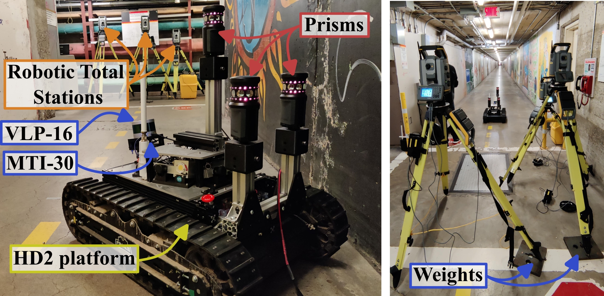
Figure 2: Setup used in the tunnel sites. Left: RTS setup with the HD2 robot. Right: one deployment done in a $120\text{\,}\mathrm{m}$ tunnel. Because the floor was slippery, heavy weights were added to stabilize the RTS tripods.

The first ground truth setup is composed of three Trimble S7 RTS. Each RTS tracks a single Trimble MultiTrack Active Target MT1000 prism at a maximum achievable measurement rate of $2.5\text{\,}\mathrm{Hz}$. For this active prism, the nominal range at the tracking mode is $800\text{\,}\mathrm{m}$ and the nominal position measurement accuracy is $4\text{\,}\mathrm{mm}$. To collect the data from each RTS, a Raspberry Pi 4 is used as a client through a USB connection. The data are then sent to a master Raspberry Pi 4 through LoRa Shield radio modules from Dragino operating with a radio frequency of $905\text{\,}\mathrm{MHz}$. The chosen modulation allows the Raspberry Pi to reliably send data over a distance of up to $800\text{\,}\mathrm{m}$ at $366\text{\,}\mathrm{Bps}$ in open space. The second ground truth setup is composed of a set of four GNSS receivers used for outdoor experiences. In this setup, three GNSS receivers are mounted on the Warthog UGV and the fourth GNSS receiver serves as a static base station. For the sake of comparison, two different models of GNSS receivers are used in this dataset, Reach RS+ and Trimble R10-2. When operating in RTK rover/base mode, the Trimble R10-2 receiver has a vertical accuracy of $21.2\text{\,}\mathrm{mm}$ and horizontal accuracy of $11.3\text{\,}\mathrm{mm}$, while the Reach RS+ has a vertical accuracy of $19.8\text{\,}\mathrm{mm}$ and horizontal accuracy of $9.9\text{\,}\mathrm{mm}$. All three prisms and GNSS receivers were mounted on the Warthog robot for outdoor experiments. The HD2 UGV was used to collect data in the university tunnels. In such environments, GNSS receivers are not functional, thus, only the prisms can be used.

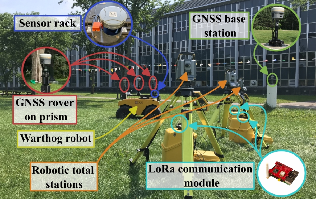
Figure 3: Setup used on the campus with the Warthog UGV. A GNSS fixed base station sends corrections to the three GNSS rovers on the robot. Three prisms are tracked by three RTS. Data are collected by three Raspberry Pi clients connected by USB to the RTS. A LoRa communication protocol is used to send data to a Raspberry Pi master located on the UGV. The lidar and IMU are on the front part of the Warthog.

IV Data collection

Our main contribution revolves around delivering a dataset featuring openly available ground truth trajectories obtained using diverse setups. The RTS-GT dataset was gathered across three distinct environmental settings, encompassing various times of day and spanning around diverse weather conditions, summarized in the Table II.

TABLE II: Table of deployments in the RTS-GT dataset. The weather legend is as follows: C=Clear, FR=Freezing rain, S=Snow, R=Rain. The robot legend means W=Warthog and H=HD2.

	Month	Exp.	Length	Weather	Robot	Setup
	Feb. 22	1	$1.58\text{\,}\mathrm{km}$	C	W	RTS/GNSS
	Mar. 22	6	$7.45\text{\,}\mathrm{km}$	FR, S, C	W	RTS/GNSS
	May 22	8	$14.43\text{\,}\mathrm{km}$	C	W	RTS/GNSS
Campus	Jun. 22	4	$3.42\text{\,}\mathrm{km}$	C	W	RTS/GNSS
	Jul. 22	6	$2.67\text{\,}\mathrm{km}$	C	W	RTS/GNSS
	Nov. 22	14	$3.91\text{\,}\mathrm{km}$	C	W	RTS/GNSS
	Dec. 22	4	$2.1\text{\,}\mathrm{km}$	C, R	W	RTS/GNSS
	Jul. 23	2	$2\text{\,}\mathrm{km}$	C	W	RTS/GNSS
	May 22	6	$1.55\text{\,}\mathrm{km}$	C	H	RTS
Tunnel	Jul. 22	5	$1.58\text{\,}\mathrm{km}$	C	H	RTS
	Sep. 22	9	$0.85\text{\,}\mathrm{km}$	C	H	RTS
Forest	Nov. 22	4	$3.16\text{\,}\mathrm{km}$	C	W	RTS/GNSS

IV-A Environments

The first deployment site is the campus of Université Laval in Quebec City. This campus comprises buildings, open spaces, and wooded areas. Multiple views of the campus are depicted in Figure 1-right and Figure 3. Overall, $45$ different experiments through $20$ distinct deployments were conducted with the Warthog UGV, totaling $37.6\text{\,}\mathrm{km}$ of trajectories on the campus. During these data collection campaigns, various weather conditions were encountered, including clear weather, rain, and even a snowstorm. Data from both RTS and GNSS setups are available for each of the conducted experiments, enabling a comparison of their respective accuracies in generating reference trajectories.

For the second deployment site, underground tunnels located beneath the university campus were selected. Four deployments were conducted in these tunnels to gather data from RTS setup during $20$ different experiments, covering a total of $4\text{\,}\mathrm{km}$ of trajectories with the HD2 platform. These tunnels have lengths of several hundred meters, which might cause particular challenges for SLAM algorithms. Unlike other setups based on motion capture or ultra-wideband, our RTS setup can generate reference trajectories at long ranges without the need to alter the environment. The Figure 2 shows an example of a tunnel as a long-range environment.

Finally, the last site is located in the Montmorency Forest, which belongs to Université Laval. This site contains numerous paths for snowmobiles and cross-country ski trails in a dense forest. Two deployments were carried out with the Warthog robot, along with RTS and GNSS systems. In total, $3.2\text{\,}\mathrm{km}$ of trajectories were acquired during four different experiments. An example of the RTS system in the forest is depicted in Figure 1-left. The lidar was available during the majority of deployments to collect data for SLAM algorithms.

IV-B Ground truth protocol

In this section, we introduce the standardized protocols that we employed for each of the setups during all conducted deployments, split between RTS and GNSS. Starting with RTS protocol, the field deployment of the three RTS is carried out in several steps:

1. ($30\text{\,}\mathrm{min}$) RTS units are acclimated to the ambient temperature before data collection can begin. This step is necessary to prevent any condensation effects that could bias the measurements, especially in winter;

2. ($5$-$60\text{\,}\mathrm{min}$) Tripods for the RTS are set up, while the RTS units adjust to the ambient temperature;

3. ($10$-$15\text{\,}\mathrm{min}$) RTS units are mounted on tripods, and we roughly level RTS units visually. To achieve a finer leveling for RTS units, calibrated electronic sensors are utilized;

4. ($3$-$5\text{\,}\mathrm{min}$) Raspberry Pi devices are powered on and connected via USB to the RTS units to retrieve their data and send it to the master unit for recording. These Raspberry Pi devices also assign a unique prism number to each RTS unit to be tracked;

5. ($1$-$2\text{\,}\mathrm{min}$) Active prisms are mounted on the UGV and powered on with their unique ID. To facilitate data processing of multiple experiments conducted by the robots, the same prism ID and positions were adopted during all data acquisition operations;

6. ($1$-$10\text{\,}\mathrm{min}$) Verification of proper prism tracking is performed, followed by measurements of static prism positions to enable post-processing extrinsic calibration of RTS units.

The complete setup process takes between $50\text{\,}\mathrm{min}$ and $120\text{\,}\mathrm{min}$, which depends on the number of available operators and weather conditions. At the end of the data collection procedure, prisms have to remain on the UGV to immediately perform an extrinsic sensor calibration, discussed later.

As for the GNSS protocol, we need a minimum of three GNSS receivers as rover plus one GNSS receiver as a base station to generate a six-DOF ground truth with only GNSS-based setup. This rover/base configuration, known as RTK, can achieve centimeter-level accuracy by correcting errors of the GNSS receivers used as rovers. The base station, consisting of a GNSS receiver, provides corrections for the rover GNSS observations by simultaneously monitoring the same satellites as the rover receivers. The base station can be fixed at a predetermined, known, and stationary location (e.g., a geodesic pillar stock or a geodetic survey marker) or an unknown position. If the position of the base station is known in advance, GNSS receivers have just to be powered on and once the radio connection between the base and rovers is established the system is operational and the collection of data can start. On the other hand, if the position of the base station is unknown, a waiting time of at least $15\text{\,}\mathrm{min}$ is necessary before data collection to let the rover or the base receivers have enough time to boot, average their positions, and achieve optimal reading of the satellite constellations in the sky. The positional corrections are then transmitted through messages via a radio link from the base station to the rover receivers, where they are employed to correct the real-time positions of the rover. Moreover, the internal radio of the GNSS receiver has a maximum range of $2\text{\,}\mathrm{km}$. To achieve a greater range, we have to use the external radio, which can theoretically transmit up to $10\text{\,}\mathrm{km}$ under optimal conditions.

IV-C Calibration and time synchronization

This section specifies how the systems were calibrated and synchronized, along with the data format given by the dataset. Attention is given to 1) extrinsic calibration and 2) time synchronization. First, the extrinsic calibration process involves obtaining the precise pose of all the sensors on the robots. Calibration is performed using one RTS at the end of each deployment to closely match the conditions of the experiments as temperature, pressure, and humidity can affect measurements, especially in winter. Retro-reflective targets, as shown in Figure 3, are stuck atop the lidar and GNSS receivers. The prisms are left in active mode for this calibration. Ten repetitions are performed for each millimeter-precise position to increase precision and to determine their uncertainties. This method provides the relative positions of the prisms, GNSS receivers, and lidar to each other. Since the IMU is too small, its extrinsic calibration with the lidar is based on the work of [19], who uses lidar and IMU data to perform calibration within a tenth of a degree using a modified four-DOF SLAM algorithm. Translation between the lidar and IMU is determined using the Computer-Aided Design (CAD) model of their support. These calibrations were performed after each deployment to ensure precise referenced measurements. As for time synchronization, a Network Time Protocol (NTP) daemon was used to synchronize the clocks between the two on-board computers on the robot (i.e., the main computer of the UGV and the Raspberry Pi master connected to the robot network). Ten minutes was allowed after booting up both of the computers so that the client clock could adjust. Measurements from the wheel encoders, lidar, and IMU were timestamped using the data logging computer’s clock. Synchronization between the master and client Raspberry Pi is achieved using a modified NTP protocol designed for LoRa communication, as described in [20]. Initial synchronization is performed at the start of data collection, followed by repetitions every five minutes for each client. This method ensures clock precision at the level of one to two milliseconds. As the GNSS devices are not connected to the setup, temporal synchronization to the RTS data is established using a classical maximum likelihood state estimator, similar to the approach taken by [17].

IV-D Data format

For each deployment and experiment, ROS 2 rosbag files are provided for data gathered by the Warthog and HD2 UGV. These files include lidar scans, IMU measurements, motors and encoders data, as well as rigid transformation between all sensor frames. Unified Robot Description Format (URDF) files are provided along with these rosbag files for each UGV. Note that no INS were used to process the IMU measurements. All IMU raw data is available in the different rosbag files. With the RTS setup, prism positions, and time synchronizations are provided for rosbag files in ROS 1 and ROS 2. The static prism positions computed for the RTS extrinsic calibration are given in a text file GCP.txt, and the sensor extrinsic calibration results are given in another text file calibration_raw.txt. Finally, NMEA and UBX files are provided for all GNSS receivers used during experiments. The RTS-GT dataset is available at https://github.com/norlab-ulaval/RTS_project, along with a toolbox code to process the data.

V Discussion and challenges

To assess the disparities among the setups, we conducted an analysis of $27$ outdoor experiments, covering a total distance of $20.6\text{\,}\mathrm{km}$, during which we tracked the trajectories of the robot using GNSS and RTS-based setups when available. We evaluated the precision of each system by employing inter-distances between prisms and GNSSs. These distances are calculated between every synchronized triplet of prism positions or GNSS receiver positions recorded during each experiment, respectively referred as inter-prism distances and inter-GNSS distances. Subsequently, each of these distance triplets is compared to their corresponding calibrated distance (evaluated at step six of our protocol) and taken as a reference to obtain the errors in precision. Furthermore, we employed an inter-precision distance to quantify variation in precision between different experiments conducted on the same site at different times. The purpose of this distance is to highlight the reproducibility of the different setups to generate ground truth trajectories. Sets of closest positions in the ground truth trajectories recorded during separate experiments are computed by a nearest neighbors algorithm. Subsequently, the inter-precision distance is computed for each set by subtracting each average inter-prism or inter-GNSS distances of each position.

V-A Precision and reproducibility

Results of inter-prism distances, inter-GNSS distances, and precision on the final translation and rotation of the robot are shown in Table III for $15$ deployments. The precision on the final pose is estimated by the same method used in our previous work [12]. It can be seen that RTS precision is stable in multiple environments, while the GNSS can have a variation of more than $300\text{\,}\mathrm{m}\mathrm{m}$ in the forest environment, as well as in open space. Moreover, higher distances between a prism and its RTS affect the precision, leading to higher uncertainties.

TABLE III: Median values for different metrics obtained over $15$ RTS and GNSS setups. All deployments happened during 2022 and the date format is day/month. For each row, light colors indicate low values, whereas dark means high values.

	Environment
1pt]2-Z	Open space									Building		Forest
	24/02	07/03	14/03	16/03	22/06	30/06	11/07	29/11	05/12	12/03	16/11	31/03	09/11	10/11	24/11
[0.5pt] Inter-prism distance [mm]	6.5	$2.4$	4.1	4.1	9.7	5.7	22.9	4.6	3.7	4.3	4.5	6.6	18.0	5.0	3.2
Inter-GNSS distance [mm]	5.5	$5.2$	4.6	6.4	37.2	368.0	111.0	6.9	20.5	230.0	17.7	288.0	149.0	394.0	423.0
Translation error [mm]	15.2	$28.7$	25.3	10.6	12.3	12.8	35.2	22.9	12.7	23.7	12.0	19.0	12.8	6.7	21.0
Rotation error [deg]	1.51	$1.6$	2.05	1.4	0.9	0.94	4.0	1.94	1.33	1.93	0.85	1.06	0.97	0.53	1.59
RTS Range [m]	39.0	$20.0$	18.0	19.0	90.0	32.0	87.0	39.0	32.0	71.0	42.0	38.0	42.0	59.0	37.4

The results depicted in Figure 4-Left offer general insights into the errors associated with the inter-prism and inter-GNSS distances. These findings reveal that the RTS acquisition system consistently achieves a median precision of approximately $4.5\text{\,}\mathrm{mm}$, whereas the GNSS system exhibits a $22$ times lower median precision, being around $118.1\text{\,}\mathrm{mm}$. It is important to emphasize that the inter-distance errors highlight the highest precision of the RTS acquisition system compared to the GNSS system. This discrepancy can be attributed to the relatively low error inherent to the RTS acquisition system, in contrast to the absolute error associated with GNSS.

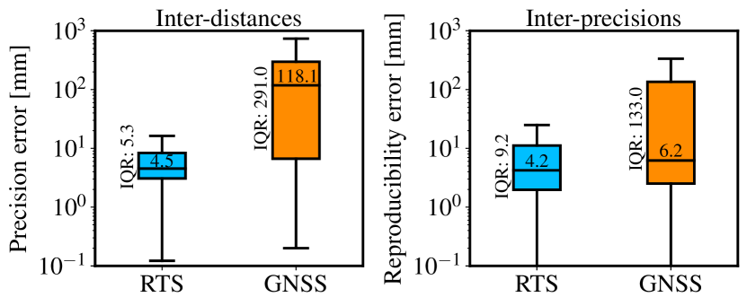
Figure 4: Distribution of errors arising for the two setups. Left: inter-prism and inter-GNSS distances. Right: inter-precision distances. Results obtained from the RTS are denoted in blue, whereas those from the GNSS are shown in orange. The median error values are in the center of each box, and the IQR is indicated alongside for reference.

To evaluate the reproducibility between experiments, we employ a nearest neighbor distance calculation within three meters, with data expressed in the GNSS frame. As illustrated in Figure 4-Right, the RTS setup consistently exhibits high reproducibility, with a median error of $4.2\text{\,}\mathrm{mm}$. The GNSS have the same level of reproducibility, with a median of $6.2\text{\,}\mathrm{mm}$. However, the GNSS IQR, with a value of $133\text{\,}\mathrm{mm}$, is $14$ times more important than the RTS. This observation underscores the stability of precision across all experiments for the RTS compared to the GNSS.

V-B Challenges encountered

The first encountered challenge was the leveling of the RTS in winter. It is sometimes necessary to remove snow from the ground for step two of our protocol to prevent tripods from gradually sinking into the snow, which would impact the ground truth. In forested areas where the snow depth can reach several meters, as shown in Figure 5-Left, surface snow is compacted to provide stability. Secondly, as depicted in Figure 1, obstacles between prisms and RTS can disrupt measurements. To address this issue, RTS placement locations are pre-selected based on the planned trajectory of the UGV, and the heights of both RTS and prisms are varied to minimize occlusion risks. Another challenge is the presence of dust or dirt on RTS lenses, as shown in Figure 5-Middle, which can degrade RTS performance. Therefore, lenses should be wiped regularly. Furthermore, since prisms and GNSS units are elevated on the UGV, they are susceptible to vibrations during motions. These vibrations can lead to positioning errors of up to $1\text{\,}\mathrm{cm}$. To deal with this problem, metal supports have been added to dampen vibrations, as depicted in Figure 5-Right. Finally, unlike GNSS data, RTS measurement timestamps are not globally valid. To address this issue and obtain the six-DOF pose, data interpolation is performed. This interpolation can reduce the accuracy of the final estimated pose, especially for high UGV dynamic and low-rate measurement setups.

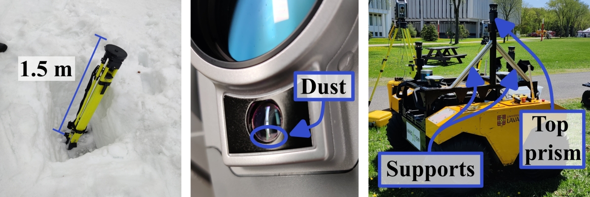
Figure 5: Issues encountered while collecting the dataset. Left: difficulties of leveling on deep snow. Middle: dust on a lens which was interfering with the tracking mode of the RTS. Right: supports added on the Warthog to reduce vibrations on the top prism.

VI Conclusion

In this paper, we have introduced a novel dataset, the RTS-GT dataset, designed to compare various ground truthing setups. The RTS-GT dataset stands out as a unique dataset for providing six-DOF reference trajectories of a moving robotic platform generated by three RTS. The dataset encompasses GNSS and RTS data as well, along with information from lidar, IMU, and encoder sensors. It facilitates the application of SLAM algorithms and the assessment of results to the ground truth data. Furthermore, the RTS-GT dataset covers diverse environments and weather conditions to assess the quality of the different ground truth setups. Additionally, tools for quantifying their precision are provided, a feature not present in previous datasets. An extensive analysis of the precision and reproducibility of different trajectory generation setups was conducted. The results indicate that RTS systems deliver more precise and reproducible data compared to GNSS solutions, even when used in RTK mode. These results demonstrate the challenges posed by generating six-DOF ground truth trajectories in outdoor and indoor environments. Moreover, it shows that multiple RTS can be used to benchmark six-DOF SLAM algorithm comparisons.

References

- [1] Li Qingqing, Yu Xianjia, Jorge Peña Queralta and Tomi Westerlund “Multi-Modal Lidar Dataset for Benchmarking General-Purpose Localization and Mapping Algorithms” In IEEE/RSJ International Conference on Intelligent Robots and Systems (IROS), 2022, pp. 3837–3844 DOI: 10.1109/IROS47612.2022.9981078
- [2] David Schubert et al. “The TUM VI Benchmark for Evaluating Visual-Inertial Odometry” In IEEE/RSJ International Conference on Intelligent Robots and Systems (IROS), 2018, pp. 1680–1687 DOI: 10.1109/IROS.2018.8593419
- [3] Yukyung Choi et al. “KAIST Multi-Spectral Day/Night Data Set for Autonomous and Assisted Driving” In IEEE Transactions on Intelligent Transportation Systems 19.3, 2018, pp. 934–948 DOI: 10.1109/TITS.2018.2791533
- [4] Dan Barnes et al. “The Oxford Radar RobotCar Dataset: A Radar Extension to the Oxford RobotCar Dataset” In IEEE International Conference on Robotics and Automation (ICRA), 2020, pp. 6433–6438 DOI: 10.1109/ICRA40945.2020.9196884
- [5] Nicholas Carlevaris-Bianco, Arash K. Ushani and Ryan M. Eustice “University of Michigan North Campus long-term vision and lidar dataset” In International Journal of Robotics Research 35.9, 2015, pp. 1023–1035
- [6] Andreas Geiger, Philip Lenz and Raquel Urtasun “Are we ready for autonomous driving? The KITTI vision benchmark suite” In IEEE Conference on Computer Vision and Pattern Recognition, 2012, pp. 3354–3361 DOI: 10.1109/CVPR.2012.6248074
- [7] Kamak Ebadi et al. “Present and Future of SLAM in Extreme Environments: The DARPA SubT Challenge” In arXiv preprint arXiv:2208.01787, 2022 arXiv: http://arxiv.org/abs/2208.01787
- [8] Lintong Zhang et al. “Hilti-Oxford Dataset: A Millimeter-Accurate Benchmark for Simultaneous Localization and Mapping” In IEEE Robotics and Automation Letters 8.1, 2023, pp. 408–415 DOI: 10.1109/LRA.2022.3226077
- [9] Jeffrey Delmerico et al. “Are We Ready for Autonomous Drone Racing? The UZH-FPV Drone Racing Dataset” In International Conference on Robotics and Automation (ICRA), 2019, pp. 6713–6719 DOI: 10.1109/ICRA.2019.8793887
- [10] Michael Helmberger et al. “The Hilti SLAM Challenge Dataset” In IEEE Robotics and Automation Letters 7.3, 2022, pp. 7518–7525 DOI: 10.1109/LRA.2022.3183759
- [11] François Pomerleau, Ming Liu, Francis Colas and Roland Siegwart “Challenging data sets for point cloud registration algorithms” In The International Journal of Robotics Research 31.14, 2012, pp. 1705–1711 DOI: 10.1177/0278364912458814
- [12] Maxime Vaidis et al. “Uncertainty analysis for accurate ground truth trajectories with robotic total stations” In IEEE International Conference on Intelligent Robots and Systems (IROS), 2023
- [13] Carlos Campos, Jose M.M. Montiel and Juan D. Tardos “Inertial-Only Optimization for Visual-Inertial Initialization” In IEEE International Conference on Robotics and Automation (ICRA) IEEE, 2020 DOI: 10.1109/icra40945.2020.9197334
- [14] Maxime Vaidis et al. “Extrinsic calibration for highly accurate trajectories reconstruction” In IEEE International Conference on Robotics and Automation (ICRA), 2023, pp. 4185–4192 DOI: 10.1109/ICRA48891.2023.10160505
- [15] Joshua Knights et al. “Wild-Places: A Large-Scale Dataset for Lidar Place Recognition in Unstructured Natural Environments” In IEEE International Conference on Robotics and Automation (ICRA), 2023, pp. 11322–11328 DOI: 10.1109/ICRA48891.2023.10160432
- [16] Holger Caesar et al. “nuScenes: A Multimodal Dataset for Autonomous Driving” In IEEE/CVF Conference on Computer Vision and Pattern Recognition (CVPR), 2020, pp. 11618–11628 DOI: 10.1109/CVPR42600.2020.01164
- [17] Michael Burri et al. “The EuRoC micro aerial vehicle datasets” In The International Journal of Robotics Research 35.10, 2016, pp. 1157–1163 DOI: 10.1177/0278364915620033
- [18] Mohinder S Grewal, Lawrence R Weill and Angus P Andrews “Global positioning systems, inertial navigation, and integration” John Wiley & Sons, 2007
- [19] Vladimír Kubelka, Maxime Vaidis and François Pomerleau “Gravity-constrained point cloud registration” In IEEE/RSJ International Conference on Intelligent Robots and Systems (IROS), 2022, pp. 4873–4879 DOI: 10.1109/IROS47612.2022.9981916
- [20] Maxime Vaidis, Philippe Giguère, François Pomerleau and Vladimír Kubelka “Accurate outdoor ground truth based on total stations” In 18th Conference on Robots and Vision (CRV), 2021, pp. 1–8 DOI: 10.1109/CRV52889.2021.00012