Product states optimize quantum $p$-spin models for large $p$

Abstract

We consider the problem of estimating the maximal energy of quantum $p$-local spin glass random Hamiltonians, the quantum analogues of widely studied classical spin glass models. Denoting by $E^{*}(p)$ the (appropriately normalized) maximal energy in the limit of a large number of qubits $n$, we show that $E^{*}(p)$ approaches $\sqrt{2\log 6}$ as $p$ increases. This value is interpreted as the maximal energy of a much simpler so-called Random Energy Model, widely studied in the setting of classical spin glasses.

Our most notable and (arguably) surprising result proves the existence of near-maximal energy states which are product states, and thus not entangled. Specifically, we prove that with high probability as $n\to\infty$, for any $E<E^{*}(p)$ there exists a product state with energy $\geq E$ at sufficiently large constant $p$. Even more surprisingly, this remains true even when restricting to tensor products of Pauli eigenstates. Our approximations go beyond what is known from monogamy-of-entanglement style arguments—the best of which, in this normalization, achieve approximation error growing with $n$. Our results not only challenge prevailing beliefs in physics that extremely low-temperature states of random local Hamiltonians should exhibit non-negligible entanglement, but they also imply that classical algorithms can be just as effective as quantum algorithms in optimizing Hamiltonians with large locality—though performing such optimization is still likely a hard problem.

Our results are robust with respect to the choice of the randomness (disorder) and apply to the case of sparse random Hamiltonian using Lindeberg’s interpolation method. The proof of the main result is obtained by estimating the expected trace of the associated partition function, and then matching its asymptotics with the extremal energy of product states using the second moment method.

Important note about error in this draft: There is an error in the proof of the current draft with regards to the upper bound in Section 5. The argument stated in this sentence is incorrect: “By choosing nearest anticommuting pairs of Pauli operators, then, one can uniquely match permutations in a way such that all contributions cancel.” Consequently, the main result in this paper may not be correct as stated. We have left the paper as-is to document the other results and will update this draft when corrections have been made to the proof and main result.

1 Introduction

We consider the quantum analogue of a classical $p$-spin glass model [BM80, ES14, BS20], which is a $p$-local random Hamiltonian taking the form

$$H_{n,p}={n\choose p}^{-1/2}\sum_{\begin{subarray}{c}\sigma\in\mathcal{P}_{n}\\ \sigma\text{ is $p$-local}\end{subarray}}\alpha_{\sigma}\sigma,\quad\quad\alpha_{\sigma}\sim\mathcal{N}(0,1),$$

where $\mathcal{P}_{n}$ denotes the set of Pauli matrices on $n$ qubits and $\alpha_{\sigma}$ are i.i.d. Gaussian coefficients (see the more formal definition in Equation 1 below).

Unlike the widely studied classical spin glass model which is now rigorously analyzed and well understood, its quantum counterpart remains notably underdeveloped. Specifically, we investigate the problem of estimating the normalized ground energy of this quantum model. For classical spin glasses, seminal developments originating from the work of Parisi [Par79] and later formalized by Talagrand and Panchenko [Tal06, Pan13], provide a remarkably precise answer to this question for every fixed $p$ via a solution of a certain variational problem. The answer simplifies dramatically as $p$ increases (after the number of spins diverges) to the value $\sqrt{2\log 2}$, as was shown recently in [GJK23]. However, quantum models of spin glasses present substantial challenges for which a rigorous analogue of Parisi’s ansatz is yet to be developed. Here we solve this problem in the large $p$ regime by establishing that the ground state value $E^{*}_{n}(p)$ of the model given in Equation 1 (normalized by $\sqrt{n})$ approaches $\sqrt{2\log 6}$ in the double limit of $n\to\infty$ and then $p\to\infty$, thus establishing a quantum analogue of the result in [GJK23]. The limit value $\sqrt{2\log 6}$ is interpreted as an extreme value of an uncorrelated sequence of Gaussians and arises naturally in the so-called Random Energy Model (REM)—a tractable simplification of classical spin glasses.

Our most important and (arguably) surprising structural result is the following implication of knowing the asymptotic value $\lim_{p}\lim_{n}E_{n}^{*}(p)=\sqrt{2\log 6}$: this value is achieved asymptotically by unentangled (that is, product) states up to an arbitrary level of precision. Specifically, for every $E<\sqrt{2\log 6}$ and large enough $p$ and $n$ there exists a product state with energy at least $E$. We thus summarize our main finding as follows:

The gap between the average limiting ground energy and the optimal energy achievable by unentangled states vanishes for random $p$-local spin glass quantum Hamiltonians when $p$ is large.

In fact, as we will show, the product states achieving near optimality take the simple form of tensor products of eigenstates of Pauli operators. This result is of potential interest in the field of condensed matter physics as it challenges conventional assumptions in physics regarding entanglement and real-world quantum systems. Namely, commonly held beliefs in physics stipulate that (a) random local Hamiltonians accurately model physical quantum systems, and that (b) low-energy states in thermal equilibrium should be entangled. Our results contradict this, revealing that for large enough $p$ and $n$, product states can achieve near-optimal energy levels. This calls into question the simultaneous validity of the stipulations (a) and (b).

Our work also has implications for quantum computational complexity, especially concerning the role of entanglement as a computational resource. The algorithmic task of finding the ground energy of a general local quantum Hamiltonian is at the heart of quantum computation theory. Not only is this problem a leading candidate to test the capabilities and limits of quantum computation, it is also a paradigmatic problem for ascertaining quantum advantage in general. Specifically, the worst-case version of our Hamiltonian (Equation 1) is QMA-complete, and thus under a widely held complexity theoretic belief such ground states cannot be efficiently classically verified (that is, $\textsc{QMA}\neq\textsc{NP}$). Our result implies that for random Hamiltonians this is not the case. Indeed, as we will show, the product states achieving near optimality are in fact Pauli basis states. As such they can be easily evaluated by classical algorithms. Thus random Hamiltonians of the form of Equation 1 do not represent the most difficult instances for quantum computation. This stands in stark contrast with the classical case where there is mounting evidence that spin glasses are in fact algorithmically hard; potentially as hard as NP-hard problems. See below for the discussion on algorithmic intractability of classical spin glasses.

Informal statement of results

We now formally define our model of quantum spin glass. The random quantum $p$-spin-glass Hamiltonian we consider takes the form

$$H_{n,p}=\frac{1}{\sqrt{{n\choose p}}}\sum_{\begin{subarray}{c}i_{1}<\cdots<i_{p}\in[n]\\ a_{1},\dots,a_{p}\in\{1,2,3\}\end{subarray}}\alpha[i_{1},\dots,i_{p};a_{1},\dots,a_{p}]\;\sigma_{i_{1}}^{a_{1}}\sigma_{i_{2}}^{a_{2}}\cdots\sigma_{i_{p}}^{a_{p}},\quad\alpha[i_{1},\dots,i_{p};a_{1},\dots,a_{p}]\sim\mathcal{N}(0,1).$$ (1)

In the above, $\alpha[i_{1},\dots,i_{p};a_{1},\dots,a_{p}]$ are i.i.d. standard normal coefficients and $\sigma_{i}^{a}$ indicates Pauli matrix $\sigma^{a}$ acting on qubit $i$ where $1,2,3$ correspond to standard Pauli operators $X,Y,Z$ respectively. We will later demonstrate that there is some flexibility in the choice of distribution for $\bm{\alpha}$. This model is inspired by its classical counterparts [SK75, Par79, EA75, Tal06] taking the diagonal Hamiltonian form

$$H_{n,p}^{c}=n^{-\frac{p-1}{2}}\sum_{i_{1},\dots,i_{p}=1}^{n}J_{i_{1},\dots,i_{p}}\sigma_{i_{1}}^{3}\cdots\sigma_{i_{p}}^{3},$$ (2)

where $J_{i_{1},\dots,i_{p}}$ are also i.i.d. standard normal coefficients.

Where convenient, we will adopt the shortened notation with super-indices $\bar{\bm{i}}=(i_{1},\ldots,i_{p})\in[n]^{p}$ and $\bar{\bm{a}}=(a_{1},\ldots,a_{p})\in\{1,2,3\}^{p}$ which are each vectors of length $p$. Letting $\mathcal{I}_{p}^{n}=\{\bar{\bm{i}}\in[n]^{p}:i_{1}<i_{2}<\cdots<i_{p}\}$ denote the set of ordered $p$-tuples, the Hamiltonian in Equation 1 can be written in the more concise form:

$$H_{n,p}=\frac{1}{{n\choose p}^{1/2}}\sum_{\bar{\bm{i}}\in\mathcal{I}_{p}^{n}}\sum_{\bar{\bm{a}}\in\{1,2,3\}^{p}}\alpha[\bar{\bm{i}};\bar{\bm{a}}]\;P_{\bar{\bm{i}}}^{\bar{\bm{a}}},$$ (3)

where $\alpha[\bar{\bm{i}};\bar{\bm{a}}]$ are i.i.d. standard normal coefficients and $P_{\bar{\bm{i}}}^{\bar{\bm{a}}}=\sigma_{i_{1}}^{a_{1}}\sigma_{i_{2}}^{a_{2}}\cdots\sigma_{i_{p}}^{a_{p}}$. When the $\bm{\alpha}$ are specified, we denote the Hamiltonian with coefficients $\bm{\alpha}$ as $H_{n,p}(\bm{\alpha})$.

An important quantity is the constant $E^{*}(p)$ corresponding to the largest average eigenvalue or maximum energy of the random Hamiltonian $H_{n,p}$ in the limit of large $n$:

$$E^{*}(p)\coloneqq\lim_{n\to\infty}\mathbb{E}\left[\frac{1}{\sqrt{n}}\lambda_{max}(H_{n,p})\right]=\lim_{n\to\infty}\mathbb{E}\left[\frac{1}{\sqrt{n}}\max_{\ket{\phi}\in\mathcal{S}_{\rm all}^{n}}\bra{\phi}H_{n,p}\ket{\phi}\right].$$ (4)

This limiting extremal value is characterized in two equivalent ways: as the largest eigenvalue $\lambda_{max}$ or as the maximum energy over the set $\mathcal{S}_{\rm all}^{n}$ of all quantum states on $n$ qubits. In fact, this average limiting energy also holds in the high probability sense (namely the model exhibits self-averaging) for any random Hamiltonian, as standard concentration bounds can be applied (see Section 3.2) to show that in the limit of large $n$, the maximum energy $\lambda_{max}(H_{n,p})$ concentrates around its average. An analogous constant $E_{\rm product}^{*}(p)$ defined as:

$$E_{\rm product}^{*}(p)\coloneqq\lim_{n\to\infty}\mathbb{E}\left[\frac{1}{\sqrt{n}}\max_{\ket{\phi}\in\mathcal{S}_{\rm product}^{n}}\bra{\phi}H_{n,p}\ket{\phi}\right]$$ (5)

quantifies the limiting maximum energy when optimizing over the set $\mathcal{S}_{\rm product}^{n}$ of all product states on $n$ qubits.

Justifying the existence of the above limits $E^{*}(p)$ and $E_{\rm product}^{*}(p)$ is far from obvious. Fortunately, for even $p$, we can extend proofs from classical spin glasses  [GT02] (see our Section 6) to show that the limit $E_{\rm product}^{*}(p)$ indeed does exist. Formally, we cannot guarantee that the limit in the definition of $E^{*}(p)$ (Equation 4) exists, and leave such a proof of existence as a conjecture (see Conjecture 5). Our formal results hold when replacing the associated $\lim$ with a $\limsup$.

Product states possess no entanglement and have efficient classical descriptions. Thus comparing $E^{*}(p)$ and $E_{\rm product}^{*}(p)$ helps answer whether extrema of the random quantum Hamiltonians are “complex” quantum states. Our main result stated informally below says that this is not the case when $p$ is large:

Theorem 1 (Main result (informal)).

The limiting maximum energy attainable by product states $E_{\rm product}^{*}(p)$ (Equation 5) as a function of locality $p$ satisfies

$$E^{*}(p)\left(1-O(1/p)\right)\leq E_{\rm product}^{*}(p)\leq E^{*}(p),$$ (6)

where $E^{*}(p)$ is the (conjectural) limit of the ground energy of the $p$-local quantum spin glass Hamiltonian (Equation 4).

Our main result therefore implies that the gap between the largest energy achieved by product states and the largest energy across all states closes as $p$ grows and thus product states achieve near optimality in the large $p$ limit. The fact that the existence of the limit $E^{*}(p)$ is yet to be justified does not impact our conclusion. Indeed, formally we establish an $n$-dependent version of Theorem 1 (see the formal statement Theorem 2 below).

In addition to the aforementioned result regarding the existence of the limit $E^{*}_{\rm product}(p)$ for every $p$, we also establish distributional insensitivity (universality) of our results with respect to the choice of randomness of $\alpha$. In particular, in Section 7 we establish that the limit $\lim_{p}E^{*}(p)=\sqrt{2\log 6}$ holds also when $\alpha$ is a zero mean sparse random variable. Here sparsity refers to the fact that the likelihood $\alpha\neq 0$ is of the order $\omega(1/n^{p-1})$, implying order $\omega(n)$ number of non-zero coefficients $\alpha$ appearing in the Hamiltonian. The term $\omega(n)$ underscores that the number of terms grows faster than $n$ at any arbitrarily slow rate. This sparsity regime corresponds to the so-called sparse random hypergraph model with “large” average degree, also called the diluted spin glass model, which was widely studied in the classical literature both in physics [FL03] and the theory of random graphs [Sen18]. To prove this result, we employ a variant of Lindeberg’s interpolation technique [Cha05], which is also the main tool underlying [Sen18].

Proof sketch

We now describe the proof idea behind Theorem 1. It is based on obtaining an upper bound on $E^{*}(p)$ and obtaining a nearly matching lower bound on $E^{*}_{\rm product}(p)$. For the upper bound we consider the expected trace of the partition function with a judicious choice of the inverse temperature of the form $\beta\sqrt{n}$ for a constant $\beta>0$. By Jensen’s inequality this provides an upper bound on the (exponent of the) largest eigenvalue. The partition function is then expanded using the Taylor series. This is in fact a standard method to analyze $H_{n,p}$, used both in [ES14, BS20] for quantum spin glasses and in [FTW19] for a related SYK model. In both cases they study the free energy with temperature on the order $O(1)$, such that the dominating terms in the Taylor expansion come from $O(1)$ powers of the Hamiltonian. In our case, as we prove, the dominating contribution comes from powers of the Hamiltonian that are linear in $n$.

Next we show that due to an underlying symmetry only commuting Pauli operators contribute non-zero values. We give a simple descripton of such operators: these are obtained simply by splitting the set of qubits $[n]$ into three parts $S_{X},S_{Y},S_{Z}$ and assigning Pauli operators $X,Y,Z$ to them respectively. From this we obtain a very simple expression for an upper bound on the expectation of the partition function given by $6^{n}\exp(\beta^{2}n/2)$. The associated bound on the largest energy is $\log\left(6^{n}\exp(\beta^{2}n/2)\right)/(\beta n)$. Optimizing over the choice of $\beta$ is how our claimed upper bound $\sqrt{2\log 6}$ is obtained.

To obtain a matching lower bound we resort to the so-called second moment method. This is done by estimating the first two moments of a certain counting quantity $Z$ and then showing that $Z\geq 1$ with high probabiltiy (whp) using the Paley–Zygmund inequality, provided the second moment nearly matches the square of the first moment. In our case the quantity of interest $Z$ is the number of high-energy states which are tensor products of single-qubit Pauli eigenstates $\ket{\psi}$ achieving normalized energy approximately $\sqrt{2\log 6}$. We are able to calculate the first and second moment of $Z$ since the energy associated with each $\ket{\psi}$ is a Gaussian with mean $0$, variance $1/n$, and covariance described in terms of the number of matching single-qubit Pauli bases between the two associated states $\ket{\psi},\ket{\psi^{\prime}}$. Note that a trivial upper bound on the first moment is obtained as the extreme of $6^{n}$ variance-$1/n$ Gaussians, which is $(1/\sqrt{n})\sqrt{2\log 6^{n}}=\sqrt{2\log 6}$. This number is then justified by controlling the second moment. Here, $6^{n}$ comes from the $3^{n}$ choices of Pauli eigenbasis for each qubit, and $2^{n}$ from the number of choices of associated eigenstates. This approach follows an approach recently developed for purely classical spin glass models with large $p$ [GJK23]. This is the special case of our model when all Paulis are restricted to be identical, which restricts the number of configurations to $2^{n}$ leading to the asymptotic maximum eigenenergy $\sqrt{2\log 2}$. As in [GJK23] we show that $E[Z^{2}]=(1+o(1))\mathbb{E}[Z]^{2}$ where $o(1)$ hides terms vanishing with $n$. The proof is obtained by saddle point approximation. The derivation is technical but conceptually simple. We also provide an alternative proof not based on saddle point approximation which achieves a weaker bound $E[Z^{2}]=O(n)\mathbb{E}[Z]^{2}$ but still obtains the claimed result by adopting a trick introduced by Frieze [Fri90] which takes advantage of concentration inequalities. This method has been used widely ever since, for example in the context of classical spin glasses in [DGZ23].

Reflecting on the proof, it reveals that for our model the ground state—namely, the energy at the edge of the spectrum—is obtained as the maximum of nearly uncorrelated Gaussians associated with product states. As a matter of fact we prove that product states typically have variance exponentially larger than random states which are typically highly entangled. Thus the intuition behind our main result may stem from this fact: entanglement reduces variance and thus entangled states have a “smaller” chance of reaching the ground state energy when compared with product states. A similar phenomenon was previously noted in [HM17], which studied worst-case bounds on product-state approximations to the ground state of sparse models. To what extent this picture extends to other types of random Hamiltonians remains to be seen.

Contradictions to prevailing intuition from physics

Our findings offer an intriguing counterpoint to widely held beliefs and conjectures in physics which hold that truly “quantum” states are needed to optimize quantum Hamiltonians. These conjectures and beliefs that stand in contrast to our findings take on various forms which we elaborate below.

First, the fact that the random quantum Hamiltonians that we study can be optimized by product states may appear especially surprising given that random states are whp nearly maximally entangled and product states form a vanishingly small portion of the set of all possible states [Pag93, FK94]. Near-ground states of random local Hamiltonians are generally not near maximally entangled as in the case of truly random states, though various works have shown that the entanglement of eigenstates of random Hamiltonians typically grows with the number of qubits either in the considered subsystem or in its boundary [VLRK03, Hua22, VR17, KLW15, LG19, Hua21]. Note that these works study eigenstates themselves and do not address how well product states approximate the ground state energy of a random Hamiltonian. Indeed, when the system has large interaction degree, monogamy of entanglement arguments can be used to show that these highly-entangled states are locally approximated by product states. [BH13] formalizes this intuition via de Finetti theorems. However, as the ground state energy of the quantum $p$-spin model scales subextensively with the number of terms—as it is extremely frustrated—the associated worst-case guarantees are unable to achieve a multiplicative-error product state approximation (with error not growing with $n$). This suggests that the product state bounds we find go beyond what can be implied from monogamy of entanglement-style arguments.

Our results also contradict so-called area laws for Hamiltonians defined on $d$-dimensional lattices, where it is conjectured that the entropy of a subsystem of a near ground state grows with the area of the boundary of such a subsystem [GHL⁺15, ECP10]. Since the Hamiltonians we study are defined on fully connected graphs (or random sparse graphs as detailed in Section 7), naively applying such an area law conjecture would lead one to believe that near ground states possess entanglement growing with the size of the subsystem itself. In fact, various papers have proposed quantum algorithms and quantum variational ansatzes to find such near ground states of the $p$-spin glass and related Hamiltonians under the belief that entanglement is beneficial in the search of such near-ground states [APD⁺06, SGS⁺22, VMC08]. Our results counter this intuition and show that, with high probability over our model class, any potential improvement in approximation by introducing entanglement is lost in the limit of large (yet constant with respect to $n$) interaction degree $p$.

Comparisons to other random quantum Hamiltonian models also stand in contrast with the main findings of our study. Indeed, [BS20] noted connections between the quantum $p$-spin model and a bosonic version of the SYK model, which numerically appeared to have a ground state satisfying a volume law [FS16]. Furthermore, our results stand in contrast with those in [CFCD⁺23] studying a sparsified GUE random Hamiltonian model consisting of $O(n^{5})$ random (nonlocal) Pauli terms each chosen completely at random from the set of all Pauli matrices. There, the authors show that near ground states of these random nonlocal Hamiltonians possess non-neglibible circuit complexity with high probability. Product states that nearly optimize the $p$-local spin glass Hamiltonians we study for large $p$, in contrast, have trivial circuit complexity since they can be constructed in a single layer.

Algorithmic (in)tractability of classical and quantum spin glasses

The fact that ground state values of quantum $p$-spin models are achievable by product states only indicates a certain kind of tractability, namely one of state representation complexity. It simply means that the near ground states can be prepared from trivial states (such as $|0\rangle^{\otimes n}$) by a constant depth (specifically depth-1) quantum circuit. Such states are called “trivial.” Triviality and non-triviality of states underlies the quantum state representation complexity questions, such as the validity of the NLTS (No-Low-Energy-Trivial-State) conjecture which was recently positively resolved in [ABN23]. By no means, however, does the triviality of near ground states imply algorithmic tractability. Namely, the algorithmic complexity of generating low energy trivial (i.e., product) states is far from clear. Recent advances based on a geometric property of solution spaces called the overlap gap property has ruled out large classes of algorithms as contenders in the classical setting—even in the setting when the disorder $\alpha$ is randomly generated as in our setting—and in fact provide strong evidence that no polynomial time algorithm exists for this problem [HS22, Gam21, GMZ22, GJK23, GJ21, GJW20].

We emphasize that our results have no bearing on, e.g., the NP-hardness of the ground-state problem for the $p$-spin glass model as NP-hardness is a statement of the worst-case complexity of the problem—our results are whp over the disorder $\bm{\alpha}$. This distinguishes this work from previous results studying product-state approximations of the ground state of $p$-spin models, which previously had been considered in a worst-case setting. [BH13] studied worst-case product-state approximations for dense $p$-local models, and give an efficient classical algorithm for finding the approximation; however, as previously mentioned, the associated guarantee on the multiplicative error grows with $n$ for the model we consider here due to its highly frustrated nature. [HM17] gives bounds for sparse models which are also loose for the model we consider. [BGKT19] also gives a constant-fraction product-state approximation for $2$-local Hamiltonians though, once again, in the worst case. [GK12] gives bounds for product-state approximations when the Hamiltonian can be written as a sum of PSD terms, and their bound loosens exponentially in $p$.

Open questions

We put forward now several open questions for future investigation. The main question of interest is whether our structural result extends for every fixed $p$ as opposed to asymptotics $p\to\infty$. Namely, is it the case that product form states achieve near optimality for every fixed $p$? We conjecture that the answer is yes. For this one would need to have a tighter control on the actual (quenched) value of the partition function as opposed to its annealed (expectation) approximation. In this direction the tools from Parisi’s ansatz [Par79],[Par80] and their rigorization by Guerra–Toninelli [GT02],[Tal06], which have been used effectively for the analysis of classical spin appear glasses, appear unavoidable. A related question is whether these product states can be restricted to be eigenstates of tensor products of Pauli operators, as is the case in the limit as $p\to\infty$. We conjecture that this is the case. Both conjectures are explicitly stated in the next Section.

Another question is whether the our result extends to other similar quantum spin models, of which the Sachdev-Ye-Kitaev (SYK) model [SY93, Ros19] is of particular importance due to its physics applications. Also of potential interest are whether our results extend to quantum analogues of classical optimization problems such as quantum versions of random $k$-SAT (denoted $k$-QSAT) [BMR09, Bra11, AKS12, LMSS09] and quantum max-cut [GP19, HNP⁺23].

Structure of the paper

The remainder of the paper is structured as follows. We formally detail our main results in Section 2. In Section 3, we prove preliminary technical results on the concentration and covariance of the energies of the Hamiltonians which we use throughout this work. Before proceeding with proofs of our main results for the quantum model, we overview our techniques for the classical $p$-spin glass model in Section 4 both to review existing results and to detail the classical nature of the proofs. Then, in Section 5, we prove Theorem 2 about the limiting maximum energy of the quantum $p$-spin model. Section 6 and Section 7 contain the proofs of the existence of the limit (Theorem 4) and the universality under different choices of distribution (Theorem 6). Finally, we study the statistical properties of entangled states in Section 8 to show entangled states typically have exponentially smaller variance in comparison with product states thus giving some intuition for our results.

2 Main results

We denote the set of $n$ elements as $[n]\coloneqq\{1,2,\dots,n\}$. Throughout this study, $n$ refers to the number of qubits. Systems of $n$ qubits live on the vector space $\mathbb{C}^{2^{n}}$. A Hamiltonian is a Hermitian matrix acting on this vector space, i.e. a matrix $H\in\mathbb{C}^{2^{n}\times 2^{n}}$ obeying the Hermitian relation $H^{\dagger}=H$. We denote the largest eigenvalue of a matrix $M$ as $\lambda_{max}(M)$.

The Pauli matrices form a basis for the space of Hermitian matrices acting on $n$ qubits. For a single qubit, there are four Pauli matrices (Paulis $I$, $X$, $Y$, and $Z$):

$$\sigma^{0}=\begin{pmatrix}1&0\\ 0&1\end{pmatrix},\quad\quad\sigma^{1}=\begin{pmatrix}0&1\\ 1&0\end{pmatrix},\quad\quad\sigma^{2}=\begin{pmatrix}0&-i\\ i&0\end{pmatrix},\quad\quad\sigma^{3}=\begin{pmatrix}1&0\\ 0&-1\end{pmatrix}.$$ (7)

For $n$ qubits, the set of Pauli matrices $\mathcal{P}_{n}$ is the set of all $4^{n}$ possible $n$-fold tensor products of Pauli matrices,

$$\mathcal{P}_{n}=\{\sigma^{a_{1}}\otimes\cdots\otimes\sigma^{a_{n}}:a_{1},\dots,a_{n}\in\{0,1,2,3\}\}.$$ (8)

If a Pauli matrix equals the identity $\sigma^{0}$ at all but a single qubit, we let $\sigma_{i}^{a}\in\mathcal{P}_{n}$ denote such a Pauli matrix where $\sigma^{a}$ acts on qubit $i$ tensored with the identity Pauli $\sigma^{0}$ on all other qubits. Given superindices $\bar{\bm{i}}=(i_{1},\ldots,i_{p})\in[n]^{p}$ and $\bar{\bm{a}}=(a_{1},\ldots,a_{p})\in\{0,1,2,3\}^{p}$, we define the Pauli matrix $P_{\bar{\bm{i}}}^{\bar{\bm{a}}}\in\mathcal{P}_{n}$ as

$$P_{\bar{\bm{i}}}^{\bar{\bm{a}}}=\prod_{k=1}^{p}\sigma_{i_{k}}^{a_{k}}.$$ (9)

As a simple example, for $n=5$ qubits, superindices $\bar{\bm{i}}=[2,4],\bar{\bm{a}}=[1,3]$ denote the Pauli matrix $P_{\bar{\bm{i}}}^{\bar{\bm{a}}}=\sigma^{0}\otimes\sigma^{1}\otimes\sigma^{0}\otimes\sigma^{3}\otimes\sigma^{0}$. Any Pauli matrix that can be written in such a form containing exactly $p$ elements in its tensor product not equal to $\sigma^{0}$ is called a $p$-local Pauli matrix. Similarly, a Hamiltonian is called a $p$-local Hamiltonian if it can be written as a linear combination of (at most) $p$-local Pauli matrices.

For $n$ qubits, we use bra-ket notation to denote states where a ket $\ket{\phi}$ is a vector in the vector space $\ket{\phi}\in\mathbb{C}^{2^{n}}$ and $\bra{\phi}$ denotes its conjugate transpose. We denote the set of all pure states by $\mathcal{S}_{\rm all}^{n}=\{\ket{\phi}\in\mathbb{C}^{2^{n}}:|\innerproduct{\phi}{\phi}|^{2}=1\}$. A state $\ket{\phi}$ is a product state on $n$ qubits if it can be written as a tensor product of states $\ket{\phi^{(i)}}$ on its individual qubits $i\in[n]$: $\ket{\phi}=\ket{\phi^{(1)}}\otimes\cdots\otimes\ket{\phi^{(n)}}$. The set of such product states on $n$ qubits we denote as

$$\mathcal{S}^{n}_{\rm product}=\{\ket{\phi}=\ket{\phi^{(1)}}\otimes\cdots\otimes\ket{\phi^{(n)}}\in\mathcal{S}_{\rm all}^{n}:\;\ket{\phi^{(i)}}\in\mathcal{S}_{\rm all}^{1},\forall i\in[n]\}.$$ (10)

A particular finite subset of $\mathcal{S}^{n}_{\rm product}$ that we will study is $\mathcal{S}^{n}_{\rm Pauli}$, the set of product states of $1$-qubit Pauli eigenstates. Pauli matrices $\sigma^{k}$ for $k\in\{1,2,3\}$ each have an eigenbasis spanned by $\ket{k,b}$ where $b\in\{+1,-1\}$ (equivalently $b\in\left\{+,-\right\}$ for shorthand) denotes the eigenstate with positive and negative eigenvalue, respectively. More explicitly, these states are:

$$\begin{split}\ket{1,+}=\frac{1}{\sqrt{2}}\begin{bmatrix}1\\ 1\end{bmatrix},\quad&\ket{1,-}=\frac{1}{\sqrt{2}}\begin{bmatrix}1\\ -1\end{bmatrix},\quad\\ \ket{2,+}=\frac{1}{\sqrt{2}}\begin{bmatrix}1\\ i\end{bmatrix},\quad&\ket{2,-}=\frac{1}{\sqrt{2}}\begin{bmatrix}1\\ -i\end{bmatrix}\\ \ket{3,+}=\begin{bmatrix}1\\ 0\end{bmatrix},\quad&\ket{3,-}=\begin{bmatrix}0\\ 1\end{bmatrix}.\end{split}$$ (11)

$\mathcal{S}^{n}_{\rm Pauli}$ is the set of all $6^{n}$ possible tensor products of these eigenstates:

$$\mathcal{S}^{n}_{\rm Pauli}=\{\ket{\phi}=\ket{\bm{a},\bm{b}}=\ket{a_{1},b_{1}}\otimes\cdots\otimes\ket{a_{n},b_{n}}\in\mathcal{S}_{\rm product}^{n}:a_{1},\dots,a_{n}\in\{1,2,3\},b_{1},\dots,b_{n}\in\{+,-\}\}.$$ (12)

We call these states Pauli basis states.

We now introduce the following $n$-dependent prelimit analogues of Equation 4 and Equation 5 with respect to the same Hamiltonian $H_{n,p}$ as defined in Equation 1.

$$E^{*}_{n}(p) \coloneqq\frac{1}{\sqrt{n}}\lambda_{max}(H_{n,p})=\frac{1}{\sqrt{n}}\max_{\ket{\phi}\in\mathcal{S}_{\rm all}^{n}}\bra{\phi}H_{n,p}\ket{\phi},$$ (13)

$$E_{n,\rm prod}^{*}(p) \coloneqq\frac{1}{\sqrt{n}}\max_{\ket{\phi}\in\mathcal{S}_{\rm product}^{n}}\bra{\phi}H_{n,p}\ket{\phi}.$$ (14)

Similarly, introduce

$$E_{n,\rm Pauli}^{*}(p) \coloneqq\frac{1}{\sqrt{n}}\max_{\ket{\phi}\in\mathcal{S}_{\rm Pauli}^{n}}\bra{\phi}H_{n,p}\ket{\phi}.$$ (15)

Note the absence of the expectation operator in the definitions above. In particular $E_{n,\rm Pauli}^{*}(p)\leq E_{n,\rm prod}^{*}(p)\leq E^{*}_{n}(p)$ are random variables, with inequalities holding trivially. We will show below, however, that these random variables are highly concentrated around their means.

We now state our main result.

Theorem 2 (Main result (formal)).

For every $\epsilon>0$ there exists $p_{0}$ such that for all $p\geq p_{0}$ the following holds with high probability with respect to the randomness of $\alpha=\left(\alpha[\bar{\bm{i}};\bar{\bm{a}}],\bar{\bm{i}}\in\mathcal{I}_{p}^{n},\bar{\bm{a}}\in\{1,2,3\}^{p}\right)$ as $n\to\infty$:

$$\sqrt{2\log 6}-\epsilon\leq E_{n,\rm Pauli}^{*}(p)\leq E_{n,\rm prod}^{*}(p)\leq E^{*}_{n}(p)\leq\sqrt{2\log 6}+\epsilon.$$ (16)

As stated in the introduction, we conjecture that a similar result hold for every $p$, as opposed to only in the limit as $p\to\infty$.

Conjecture 3.

For every $p$ the following holds whp as $n\to\infty$:

$$\lim_{n}E_{n,\rm Pauli}^{*}(p)/E_{n}^{*}(p)=\lim_{n}E_{n,\rm prod}^{*}(p)/E_{n}^{*}(p)=1.$$ (17)

Next we turn to our results regarding the existence of limits of random variables $E^{*}_{n}(p)$, $E_{n,\rm prod}^{*}(p)$, and $E_{n,\rm Pauli}^{*}(p)$. While we leave open the question of the existence of the limit of $E^{*}_{n}(p)$, we can confirm these limits for the latter variables.

Theorem 4.

For every even $p$ there exist constants $E^{*}_{\rm prod}(p)$ and $E_{\rm Pauli}^{*}(p)$ such that whp as $n\to\infty$, $E_{n,\rm prod}^{*}(p)\to E^{*}_{\rm prod}(p)$ and $E_{n,\rm Pauli}^{*}(p)\to E_{\rm Pauli}^{*}(p)$.

The status of this question for $E^{*}_{n}(p)$ remains a conjecture.

Conjecture 5.

For every $p$ there exist constants $E^{*}(p)$ such that whp as $n\to\infty$, $E_{n}^{*}(p)\to E^{*}(p)$.

Finally, we turn to our universality results. Namely, insensitivity with respect to the choice of distribution of the disorder $\alpha$. We consider a sequence of centered variance $1$ distributions $\mathcal{D}_{n}$ with the following properties. Let $X_{n}$ be distributed according to $\mathcal{D}_{n}$. Then:

$$\mathbb{E}[X_{n}]=0,$$

$$\mathbb{E}[X_{n}^{2}]=1,$$

$$\forall\epsilon>0,\;\lim_{n\to\infty}\mathbb{E}[X_{n}^{2};|X_{n}|>n^{(p-1)/2}\epsilon]=0.$$ (18)

Theorem 6 (Universality).

Suppose the coefficients ${\bm{\alpha}}=\left(\alpha[\bar{\bm{i}};\bar{\bm{a}}],\bar{\bm{i}}\in\mathcal{I}_{p}^{n},\bar{\bm{a}}\in\{1,2,3\}^{p}\right)$ of the Hamiltonian $H_{n,p}$ are generated i.i.d. according to a distribution $\mathcal{D}_{n}$ satisfying Equation 18. Then for every $p$,

$$\lim_{n\to\infty}\mathbb{E}_{\alpha[\bar{\bm{i}},\bar{\bm{a}}]\sim\mathcal{N}(0,1)}\left[\frac{1}{\sqrt{n}}\max_{\ket{\phi}\in\mathcal{S}_{\rm all}^{n}}\bra{\phi}H_{n,p}(\bm{\alpha})\ket{\phi}\right]=\lim_{n\to\infty}\mathbb{E}_{\alpha[\bar{\bm{i}},\bar{\bm{a}}]\sim\mathcal{D}_{n}}\left[\frac{1}{\sqrt{n}}\max_{\ket{\phi}\in\mathcal{S}_{\rm all}^{n}}\bra{\phi}H_{n,p}(\bm{\alpha})\ket{\phi}\right].$$ (19)

A canonical model where our theorem above applies is the setting of a sparse random graph. Construct the distribution $\mathcal{D}_{n}$ as follows: entries of $\bm{\tilde{\alpha}}=\left(\tilde{\alpha}[\bar{\bm{i}};\bar{\bm{a}}],\bar{\bm{i}}\in\mathcal{I}_{p}^{n},\bar{\bm{a}}\in\{1,2,3\}^{p}\right)$ take values $\pm 1$ with probability $(1/2)3^{-p}d_{n}/{n\choose p-1}$ and take value $0$ otherwise, independently across $\bar{\bm{i}}$ and $\bar{\bm{a}}$. Namely, non-zero terms are supported on a sparse random hypergraph with average degree (number of non-zero disorders per node) equal to $(d_{n}3^{-p}/{n\choose p-1})3^{p}{n-1\choose p-1}=d_{n}$, where $d_{n}$ is assumed to be an arbitrarily slowly growing function of $n$. The $3^{p}$ factors account for the $3^{p}$ possible Pauli matrices on each hyperedge.

In order to bring $\tilde{\alpha}$ to the setting of Equation 18 we rescale the disorder as follows: $\alpha^{\prime}=\sqrt{{n\choose p-1}\over d_{n}}\tilde{\alpha}$. Then $\mathbb{E}[\alpha^{\prime}]=0$ and $\mathbb{E}[\alpha^{\prime 2}]=1$. We have

$$\mathbb{P}\left(\alpha^{\prime}>n^{p-1\over 2}\epsilon\right)=\mathbb{P}\left(\tilde{\alpha}>\sqrt{d_{n}(p-1)!}\epsilon+o(1)\right)$$ (20)

which becomes zero as soon as $d_{n}$ is large enough. This means that the third condition in Equation 18 holds trivially for large enough $n$ and thus Equation 19 holds. Rewriting this identity in terms of the random variables $\alpha^{\prime}=\sqrt{3^{p}{n\choose p-1}\over d_{n}}\tilde{\alpha}$ we obtain that

$$\lim_{n\to\infty}\mathbb{E}_{\alpha[\bar{\bm{i}},\bar{\bm{a}}]\sim\mathcal{N}(0,1)}\left[\frac{1}{\sqrt{n}}\max_{\ket{\phi}\in\mathcal{S}_{\rm all}^{n}}\bra{\phi}H_{n,p}(\bm{\alpha})\ket{\phi}\right]=\lim_{n\to\infty}\mathbb{E}_{\tilde{\alpha}[\bar{\bm{i}},\bar{\bm{a}}]\sim\mathcal{D}_{n}}\left[\frac{1}{\sqrt{n}}\sqrt{3^{p}{n\choose p-1}\over d_{n}}\max_{\ket{\phi}\in\mathcal{S}_{\rm all}^{n}}\bra{\phi}H_{n,p}(\bm{\tilde{\alpha}})\ket{\phi}\right].$$ (21)

Redefining the Hamiltonian $H_{n,p}$ as

$$\tilde{H}_{n,p}=\sum_{\bar{\bm{a}}\in\{1,2,3\}^{p}}\alpha^{\prime}[\bar{\bm{i}};\bar{\bm{a}}]\;P_{\bar{\bm{i}}}^{\bar{\bm{a}}}$$ (22)

we obtain a simplified identity:

$$\lim_{n\to\infty}\mathbb{E}_{\alpha[\bar{\bm{i}},\bar{\bm{a}}]\sim\mathcal{N}(0,1)}\left[\frac{1}{\sqrt{n}}\max_{\ket{\phi}\in\mathcal{S}_{\rm all}^{n}}\bra{\phi}H_{n,p}(\bm{\alpha})\ket{\phi}\right]=\lim_{n\to\infty}\mathbb{E}_{\alpha^{\prime}[\bar{\bm{i}},\bar{\bm{a}}]\sim\mathcal{D}_{n}}\left[{1\over\sqrt{nd_{n}}}\max_{\ket{\phi}\in\mathcal{S}_{\rm all}^{n}}\bra{\phi}\tilde{H}_{n,p}(\bm{\alpha}^{\prime})\ket{\phi}\right].$$ (23)

In fact, as in the classical setting, our proof implies the following double limit identity. Suppose $d$ is a constant not depending on $n$. Define the associated distribution $\mathcal{D}_{n,d}$ of the disorder as above with $d$ replacing $d_{n}$. Then

$$\lim_{n\to\infty}\mathbb{E}_{\alpha[\bar{\bm{i}},\bar{\bm{a}}]\sim\mathcal{N}(0,1)}\left[\frac{1}{\sqrt{n}}\max_{\ket{\phi}\in\mathcal{S}_{\rm all}^{n}}\bra{\phi}H_{n,p}(\bm{\alpha})\ket{\phi}\right]=\lim_{d\to\infty}\lim_{n\to\infty}\mathbb{E}_{\alpha^{\prime}[\bar{\bm{i}},\bar{\bm{a}}]\sim\mathcal{D}_{n,d}}\left[{1\over\sqrt{nd}}\max_{\ket{\phi}\in\mathcal{S}_{\rm all}^{n}}\bra{\phi}\tilde{H}_{n,p}(\bm{\alpha}^{\prime})\ket{\phi}\right],$$ (24)

which is a more common way of expressing this universality in the classical setting. We do not bother with this formal strengthening for simplicity.

3 Preliminary technical results

3.1 Variance and covariance of energies

An important quantity in our study is the covariance of the energy of the random Hamiltonian with respect to given states $\ket{\phi}$ and $\ket{\psi}$. Lemma 7 quantifies this covariance for product states and is crucially used throughout our proofs in later sections. For completeness, we also calculate variance and covariance for the energy over arbitrary and potentially entangled states in Section 8 and comment on how entanglement typically reduces the magnitude of the variance there.

Lemma 7.

For any two product states $\ket{\phi},\ket{\psi}\in\mathcal{S}_{\rm product}^{n}$ where $\ket{\phi}=\ket{\phi^{(1)}}\otimes\cdots\otimes\ket{\phi^{(n)}}$ and $\ket{\psi}=\ket{\psi^{(1)}}\otimes\cdots\otimes\ket{\psi^{(n)}}$:

$$\mathbb{E}\left[\bra{\phi}H_{n,p}\ket{\phi}\bra{\psi}H_{n,p}\ket{\psi}\right]=\frac{1}{\binom{n}{p}}\sum_{\bar{\bm{i}}\in\mathcal{I}_{p}^{n}}\prod_{k=1}^{p}\left(2\left|\bra{\phi^{(i_{k})}}\ket{\psi^{(i_{k})}}\right|^{2}-1\right).$$ (25)

Furthermore, if $\ket{\phi},\ket{\psi}\in\mathcal{S}_{\rm Pauli}^{n}$ are restricted to the Pauli eigenbasis where $\ket{\phi}=\ket{p_{1},b_{1}}\otimes\cdots\otimes\ket{p_{n},b_{n}}$ and $\ket{\psi}=\ket{p_{1}^{\prime},b_{1}^{\prime}}\otimes\cdots\otimes\ket{p_{n}^{\prime},b_{n}^{\prime}}$, then

$$\mathbb{E}\left[\bra{\phi}H_{n,p}\ket{\phi}\bra{\psi}H_{n,p}\ket{\psi}\right]=\frac{1}{\binom{n}{p}}\sum_{\bar{\bm{i}}\in\mathcal{I}_{p}^{n}:\bar{\bm{i}}\subseteq\Delta\left(\phi,\psi\right)}\prod_{k=1}^{p}b_{i_{k}}b_{i_{k}}^{\prime},$$ (26)

where $\Delta\left(\phi,\psi\right)=\{i\in[n]:p_{i}=p_{i}^{\prime}\}$ is the set of qubits in the same Pauli eigenbasis.

Proof.

By taking the expectation over coefficients, it is straightforward to note that

$$\mathbb{E}\left[\bra{\phi}H_{n,p}\ket{\phi}\bra{\psi}H_{n,p}\ket{\psi}\right]=\frac{1}{\binom{n}{p}}\sum_{\bar{\bm{i}}\in\mathcal{I}_{p}^{n}}\sum_{\bar{\bm{a}}\in\{1,2,3\}^{p}}\bra{\phi}P_{\bar{\bm{i}}}^{\bar{\bm{a}}}\ket{\phi}\bra{\psi}P_{\bar{\bm{i}}}^{\bar{\bm{a}}}\ket{\psi}.$$ (27)

Since $\ket{\phi}$ is a product state, we denote its tensor components as $\ket{\phi}=\ket{\phi^{(1)}}\otimes\cdots\otimes\ket{\phi^{(n)}}$ and similarly for $\ket{\psi}$. Looking at each term within the first sum, for each $\bar{\bm{i}}$:

$$\begin{split}\sum_{\bar{\bm{a}}\in\{1,2,3\}^{p}}\bra{\phi}P_{\bar{\bm{i}}}^{\bar{\bm{a}}}\ket{\phi}\bra{\psi}P_{\bar{\bm{i}}}^{\bar{\bm{a}}}\ket{\psi}&=\sum_{a_{1}\in\{1,2,3\}}\bra{\phi^{(i_{1})}}\sigma_{a_{1}}\ket{\phi^{(i_{1})}}\bra{\psi^{(i_{1})}}\sigma_{a_{1}}\ket{\psi^{(i_{1})}}\\ &\quad\times\sum_{a_{2}\in\{1,2,3\}}\bra{\phi^{(i_{2})}}\sigma_{a_{2}}\ket{\phi^{(i_{2})}}\bra{\psi^{(i_{2})}}\sigma_{a_{2}}\ket{\psi^{(i_{2})}}\\ &\quad\times\cdots\\ &\quad\times\sum_{a_{p}\in\{1,2,3\}}\bra{\phi^{(i_{p})}}\sigma_{a_{p}}\ket{\phi^{(i_{p})}}\bra{\psi^{(i_{p})}}\sigma_{a_{p}}\ket{\psi^{(i_{p})}}.\end{split}$$ (28)

For each individual sum on the right hand side, we have

$$\sum_{a_{k}\in\{1,2,3\}}\bra{\phi^{(i_{k})}}\sigma_{a_{k}}\ket{\phi^{(i_{k})}}\bra{\psi^{(i_{k})}}\sigma_{a_{k}}\ket{\psi^{(i_{k})}}=\bra{\phi^{(i_{k})}}\bra{\psi^{(i_{k})}}\left(\sum_{a_{k}\in\{1,2,3\}}\sigma_{a_{k}}\otimes\sigma_{a_{k}}\right)\ket{\phi^{(i_{k})}}\ket{\psi^{(i_{k})}}.$$ (29)

To continue, we must differentiate between the setting where $\ket{\phi}$ and $\ket{\psi}$ are arbitrary product states or product states in the Pauli eigenbasis.

Arbitrary product state

Defining the $\operatorname{SWAP}$ operator as

$$\operatorname{SWAP}=\begin{bmatrix}1&0&0&0\\ 0&0&1&0\\ 0&1&0&0\\ 0&0&0&1\end{bmatrix},$$ (30)

we note that

$$\sum_{a\in\{1,2,3\}}\sigma^{a}\otimes\sigma^{a}=\begin{bmatrix}0&0&0&1\\ 0&0&1&0\\ 0&1&0&0\\ 1&0&0&0\end{bmatrix}+\begin{bmatrix}0&0&0&-1\\ 0&0&1&0\\ 0&1&0&0\\ -1&0&0&0\end{bmatrix}+\begin{bmatrix}1&0&0&0\\ 0&-1&0&0\\ 0&0&-1&0\\ 0&0&0&1\end{bmatrix}=2(\operatorname{SWAP})-I.$$ (31)

Therefore, returning to Equation 29:

$$\begin{split}\bra{\phi^{(i_{k})}}\bra{\psi^{(i_{k})}}\left(\sum_{a_{k}\in\{1,2,3\}}\sigma_{a_{k}}\otimes\sigma_{a_{k}}\right)\ket{\phi^{(i_{k})}}\ket{\psi^{(i_{k})}}&=\bra{\phi^{(i_{k})}}\bra{\psi^{(i_{k})}}\left[2(\operatorname{SWAP})-I\right]\ket{\phi^{(i_{k})}}\ket{\psi^{(i_{k})}}\\ &=2\left|\bra{\phi^{(i_{k})}}\ket{\psi^{(i_{k})}}\right|^{2}-1,\end{split}$$ (32)

and thus

$$\sum_{\bar{\bm{a}}\in\{1,2,3\}^{p}}\bra{\phi}P_{\bar{\bm{i}}}^{\bar{\bm{a}}}\ket{\phi}\bra{\psi}P_{\bar{\bm{i}}}^{\bar{\bm{a}}}\ket{\psi}=\prod_{k=1}^{p}\left(2\left|\bra{\phi^{(i_{k})}}\ket{\psi^{(i_{k})}}\right|^{2}-1\right).$$ (33)

Returning to Equation 27, we now have that

$$\begin{split}\mathbb{E}\left[\bra{\phi}H_{n,p}\ket{\phi}\bra{\psi}H_{n,p}\ket{\psi}\right]&=\frac{1}{\binom{n}{p}}\sum_{\bar{\bm{i}}\in\mathcal{I}_{p}^{n}}\sum_{\bar{\bm{a}}\in\{1,2,3\}^{p}}\bra{\phi}P_{\bar{\bm{i}}}^{\bar{\bm{a}}}\ket{\phi}\bra{\psi}P_{\bar{\bm{i}}}^{\bar{\bm{a}}}\ket{\psi}\\ &=\frac{1}{\binom{n}{p}}\sum_{\bar{\bm{i}}\in\mathcal{I}_{p}^{n}}\prod_{k=1}^{p}\left(2\left|\bra{\phi^{(i_{k})}}\ket{\psi^{(i_{k})}}\right|^{2}-1\right).\end{split}$$ (34)

Product state in Pauli eigenbasis

Here, we can decompose the states into their corresponding Pauli eigenbasis and sign for each qubit, i.e., $\ket{\phi}=\ket{p_{1},b_{1}}\otimes\cdots\otimes\ket{p_{n},b_{n}}$ and $\ket{\psi}=\ket{p_{1}^{\prime},b_{1}^{\prime}}\otimes\cdots\otimes\ket{p_{n}^{\prime},b_{n}^{\prime}}$. In this setting, the right hand side of Equation 29 evaluates to

$$\bra{\phi^{(i_{k})}}\bra{\psi^{(i_{k})}}\left(\sum_{a_{k}\in\{1,2,3\}}\sigma_{a_{k}}\otimes\sigma_{a_{k}}\right)\ket{\phi^{(i_{k})}}\ket{\psi^{(i_{k})}}=\mathbbm{1}\left[p_{i_{k}}=p_{i_{k}}^{\prime}\right]b_{i_{k}}b_{i_{k}}^{\prime}.$$ (35)

Denoting $\Delta\left(\phi,\psi\right)=\{i\in[n]:p_{i}=p_{i}^{\prime}\}$ (or equivalently $\Delta\left(\bm{p},\bm{p^{\prime}}\right)$) as the set of indices in the same eigenbasis, we can simplify Equation 27 here to

$$\mathbb{E}\left[\bra{\phi}H_{n,p}\ket{\phi}\bra{\psi}H_{n,p}\ket{\psi}\right]=\frac{1}{\binom{n}{p}}\sum_{\bar{\bm{i}}\in\mathcal{I}_{p}^{n}:\bar{\bm{i}}\subseteq\Delta\left(\phi,\psi\right)}\prod_{k=1}^{p}b_{i_{k}}b_{i_{k}}^{\prime}.$$ (36)

∎

As a consequence of the above, for any product state $\ket{\phi}\in\mathcal{S}_{\rm product}^{n}$, the variance is normalized so that $\mathbb{E}\left[\bra{\phi}H_{n,p}\ket{\phi}\bra{\phi}H_{n,p}\ket{\phi}\right]=1$.

3.2 Concentration

Throughout this study, we aim to study properties of “typical” random Hamiltonians $H_{n,p}$ by studying these properties on average. In the case of the largest eigenvalue, standard Gaussian concentration inequalities can be applied to show that $\lambda_{max}(\sqrt{n}H_{n,p})$ is concentrated around its mean.

Proposition 8 (Concentration of largest eigenvalue).

For all $t\geq 0$:

$$\mathbb{P}\left[\left|\lambda_{max}(\sqrt{n}H_{n,p})-\mathbb{E}\lambda_{max}(\sqrt{n}H_{n,p})\right|\geq tn\right]\leq 2\exp\left(-\frac{t^{2}n}{2\cdot 3^{p}}\right).$$ (37)

To prove this, we apply the Gaussian concentration inequality for Lipschitz functions. A function $f:\mathbb{R}^{N}\to\mathbb{R}$ is $L$-Lipschitz if $|f(x)-f(y)|\leq L\|x-y\|_{2}$ for all $x,y\in\mathbb{R}^{n}$.

Lemma 9 (Gaussian concentration inequality for Lipschitz functions; Theorem 2.26 of [Wai19]).

Let $X_{1},\dots,X_{N}$ be i.i.d. standard Normal variables and $f:\mathbb{R}^{N}\to\mathbb{R}$ be an $L$-Lipschitz function. Then for any $t\geq 0$:

$$\mathbb{P}\left[\left|f(X)-\mathbb{E}f(X)\right|\geq t\right]\leq 2\exp\left(-\frac{t^{2}}{2L^{2}}\right).$$ (38)

Proof of Proposition 8.

Applying Lemma 9 with $f(\bm{\alpha})=\lambda_{max}(\sqrt{n}H_{n,p}(\bm{\alpha}))$, it suffices to show that the function $\lambda_{max}(\sqrt{n}H_{n,p}(\bm{\alpha}))$ has Lipschitz constant bounded by $n$. Note that for any given state $\ket{\phi}$

$$\|\nabla_{\bm{\alpha}}\bra{\phi}\sqrt{n}H_{n,p}(\bm{\alpha})\ket{\phi}\|_{2}^{2}=\frac{n}{\binom{n}{p}}\sum_{\bar{\bm{i}}\in\mathcal{I}_{p}^{n}}\sum_{\bar{\bm{a}}\in\{1,2,3\}^{p}}\left(\bra{\phi}P_{\bar{\bm{i}}}^{\bar{\bm{a}}}\ket{\phi}\right)^{2}.$$ (39)

Since $\left(\bra{\phi}P_{\bar{\bm{i}}}^{\bar{\bm{a}}}\ket{\phi}\right)^{2}\leq 1$ for any Pauli matrix $P_{\bar{\bm{i}}}^{\bar{\bm{a}}}$, this implies that $\|\nabla_{\bm{\alpha}}\bra{\phi}\sqrt{n}H_{n,p}\ket{\phi}\|_{2}^{2}\leq 3^{p}n$ and the Lipschitz constant of the function $\bra{\phi}\sqrt{n}H_{n,p}(\bm{\alpha})\ket{\phi}$ is bounded by $L\leq\sqrt{3^{p}n}$.

The function $\lambda_{max}(\sqrt{n}H_{n,p}(\bm{\alpha}))$ also has the same Lipschitz bound $L\leq\sqrt{3^{p}n}$. This can be shown by the following argument. $\lambda_{max}(\sqrt{n}H_{n,p}(\bm{\alpha}))$ is the maximum of $\bra{\phi}\sqrt{n}H_{n,p}(\bm{\alpha})\ket{\phi}$ over all states $\ket{\phi}$. For a given draw of coefficients $\bm{\alpha}$, let $\ket{\psi}$ be a state which achieves the optimum $\bra{\psi}\sqrt{n}H_{n,p}(\bm{\alpha})\ket{\psi}=\lambda_{max}(\sqrt{n}H_{n,p}(\bm{\alpha}))$; then,

$$\lambda_{max}(\sqrt{n}H_{n,p}(\bm{\alpha}))\leq\bra{\psi}\sqrt{n}H_{n,p}(\bm{\alpha}^{\prime})\ket{\psi}+L\|\bm{\alpha}-\bm{\alpha}^{\prime}\|\leq\lambda_{max}(\sqrt{n}H_{n,p}(\bm{\alpha}^{\prime}))+L\|\bm{\alpha}-\bm{\alpha}^{\prime}\|.$$ (40)

Applying a symmetric bound, we similarly have that $\lambda_{max}(\sqrt{n}H_{n,p}(\bm{\alpha}))\geq\lambda_{max}(\sqrt{n}H_{n,p}(\bm{\alpha}^{\prime}))-L\|\bm{\alpha}-\bm{\alpha}^{\prime}\|$. This then implies that $\left|\lambda_{max}(\sqrt{n}H_{n,p}(\bm{\alpha}))-\lambda_{max}(\sqrt{n}H_{n,p}(\bm{\alpha}^{\prime}))\right|\leq L\|\alpha-\alpha^{\prime}\|$, which is the same Lipschitz bound. Taking $L^{2}=3^{p}n$ in Lemma 9 completes the proof. ∎

Remark 10.

The proof of Proposition 8 can be adapted to show that the maximum energy over product states

$$E_{n,\rm Prod}^{*}(p)\coloneqq\frac{1}{\sqrt{n}}\max_{\ket{\phi}\in\mathcal{S}_{\rm product}^{n}}\bra{\phi}H_{n,p}\ket{\phi}$$ (41)

or over Pauli basis states

$$E_{n,\rm Pauli}^{*}(p)\coloneqq\frac{1}{\sqrt{n}}\max_{\ket{\phi}\in\mathcal{S}_{\rm Pauli}^{n}}\bra{\phi}H_{n,p}\ket{\phi}$$ (42)

for a random Hamiltonian is concentrated around expectations $\mathbb{E}E_{n,\rm Prod}^{*}(p)$ and $\mathbb{E}E_{n,\rm Pauli}^{*}(p)$ respectively (see Equation 5 and Equation 15). In fact, the same Lipschitz bound $L\leq\sqrt{3^{p}n}$ applies to these two quantities since $\left(\bra{\phi}P_{\bar{\bm{i}}}^{\bar{\bm{a}}}\ket{\phi}\right)^{2}\leq 1$ holds for any quantum state (see Equation 39 in proof). Therefore, we have a concentration inequality of the form:

$$\mathbb{P}\left[\left|E_{n,\rm Prod}^{*}(p)-\mathbb{E}\left[E_{n,\rm Prod}^{*}(p)\right]\right|\geq t\right]\leq 2\exp\left(-\frac{t^{2}n}{2\cdot 3^{p}}\right),$$ (43)

and similarly for the Pauli basis states.

4 Expected maximum eigenvalue in the classical $p$-spin model

Before proceeding with the quantum model, we analyze the properties of the more commonly studied classical $p$-spin model $H_{n,p}^{c}$. This model takes the form of the quantum model restricted to diagonal Pauli terms:

$$H_{n,p}^{c}=n^{-\frac{p-1}{2}}\sum_{i_{1},\dots,i_{p}=1}^{n}J_{i_{1},\dots,i_{p}}\sigma_{i_{1}}^{3}\cdots\sigma_{i_{p}}^{3}.$$ (44)

Since the above Hamiltonian is diagonal in the computational basis, we can evaluate any eigenvalue by measuring its corresponding bitstring. That is, for any $\tau\in\{-1,+1\}^{n}$, the energy of the above Hamiltonian can be written in the more standard form:

$$H_{n,p}^{c}(\tau)=n^{-\frac{p-1}{2}}\sum_{i_{1},\dots,i_{p}=1}^{n}J_{i_{1},\dots,i_{p}}\tau_{i_{1}}\cdots\tau_{i_{p}}.$$ (45)

We are interested in the expected maximum eigenvalue of this classical Hamiltonian:

$$\mathbb{E}\left[\frac{1}{n}\lambda_{max}(H_{n,p}^{c})\right]=\mathbb{E}\left[\frac{1}{n}\max_{\tau\in\{-1,+1\}^{n}}H_{n,p}^{c}(\tau)\right].$$ (46)

The results we give in this section were already demonstrated in [GJK23], though we use different techniques in proving the matching lower bound. We present these results not only for review, but also to emphasize the inherently classical nature of the near-ground states we study in our quantum model, as the techniques we use in studying the two models are near identical.

For concreteness, the result we show here is:

Theorem 11 (Classical analogue of main result).

For every $\epsilon>0$ there exists $p_{0}$ such that for all $p\geq p_{0}$ as $n\to\infty$:

$$\sqrt{2\log 2}-\epsilon\leq\mathbb{E}\left[\frac{1}{n}\lambda_{max}\left(H_{n,p}^{c}\right)\right]\leq\sqrt{2\log 2}.$$ (47)

4.1 Upper bound on the expected maximum eigenvalue

We can find an upper bound on the expected maximum eigenvalue by considering the free energy defined as

$$F(\beta)=\frac{1}{\beta}\mathbb{E}\log\left(\sum_{\tau\in\{-1,+1\}^{n}}\exp\left(\beta H_{n,p}^{c}(\tau)\right)\right).$$ (48)

The sum inside the logarithm above is denoted as the partition function. The maximum eigenvalue is related to the quantity above by the inequality

$$\mathbb{E}\left[\frac{1}{n}\lambda_{max}(H_{n,p}^{c})\right]=\frac{1}{\beta n}\mathbb{E}\log\left(\exp\left(\beta\lambda_{max}(H_{n,p}^{c})\right)\right)\leq\frac{1}{\beta n}\mathbb{E}\log\left(\sum_{\tau\in\{-1,+1\}^{n}}\exp\left(\beta H_{n,p}^{c}(\tau)\right)\right)=\frac{F(\beta)}{n}.$$ (49)

Noting that for any $\tau\in\{-1,+1\}^{n}$, the random variable $\beta H_{n,p}^{c}(\tau)$ is Gaussian with mean zero and variance $\beta^{2}n$, we have

$$\mathbb{E}\sum_{\tau\in\{-1,+1\}^{n}}\exp\left(\beta H_{n,p}^{c}(\tau)\right)=2^{n}\exp\left(\frac{1}{2}\beta^{2}n\right),$$ (50)

where each term in the sum above can be evaluated from the moment generating function of the Guassian random variable $\beta nH_{n,p}^{c}(\tau)$. Using this fact along with Jensen’s inequality yields:

$$\begin{split}\mathbb{E}\left[\frac{1}{n}\lambda_{max}(H_{n,p}^{c})\right]&\leq\frac{1}{\beta n}\mathbb{E}\log\left(\sum_{\tau\in\{-1,+1\}^{n}}\exp\left(\beta H_{n,p}^{c}(\tau)\right)\right)\\ &\leq\frac{1}{\beta n}\log\left(\mathbb{E}\sum_{\tau\in\{-1,+1\}^{n}}\exp\left(\beta H_{n,p}^{c}(\tau)\right)\right)\\ &\leq\frac{1}{\beta n}\log\left(2^{n}\exp\left(\frac{1}{2}\beta^{2}n\right)\right)\\ &=\frac{\log 2}{\beta}+\frac{\beta}{2}.\end{split}$$ (51)

Minimizing over $\beta$ then gives:

$$\mathbb{E}\left[\frac{1}{n}\lambda_{max}(H_{n,p}^{c})\right]\leq\sqrt{2\log 2}.$$ (52)

This is the upper bound claimed in Theorem 11.

4.2 Matching lower bound in the large $p$ limit

The upper bound above is true for all values of $n$ and $p$. Via the second moment method, a matching lower bound can be obtained for the limit of large $p$. We can use the second moment method applied to the number of configurations $N_{\epsilon}$ above energy threshold $(1-\epsilon)\sqrt{2\log 2}n$ for some $\epsilon\geq 0$ defined as

$$N_{\epsilon}=\left|\left\{\tau\in\{-1,+1\}^{n}:H_{n,p}^{c}(\tau)\geq(1-\epsilon)\sqrt{2\log 2}n\right\}\right|.$$ (53)

To simplify notation we introduce the constant $C_{\epsilon}\coloneqq(1-\epsilon)\sqrt{2\log 2}$. The second moment method guarantees that $N_{\epsilon}>0$ via the Paley–Zygmund inequality:

$$\mathbb{P}\left[N_{\epsilon}>0\right]\geq\frac{\mathbb{E}[N_{\epsilon}]^{2}}{\mathbb{E}{[N_{\epsilon}^{2}]}}.$$ (54)

Denoting the cumulative distribution function (CDF) of the standard normal distribution as $\Phi$, we have the following property of the tail bound for $\Phi(x)$ [Sav62]:

$$1-\Phi(x)=\frac{1}{x+O\left(\frac{1}{x}\right)}\frac{1}{\sqrt{2\pi}}\exp\left(-\frac{x^{2}}{2}\right).$$ (55)

Since $H_{n,p}^{c}(\tau)$ is Gaussian with mean zero and variance $n$ for any $\tau\in\{-1,+1\}^{n}$, the first moment is equal to

$$\begin{split}\mathbb{E}N_{\epsilon}&=\sum_{\tau\in\{-1,+1\}^{n}}\mathbb{P}[H_{n,p}^{c}(\tau)\geq C_{\epsilon}n]\\ &=2^{n}\left(1-\Phi((1-\epsilon)\sqrt{2n\log 2}\sqrt{n})\right)\\ &=2^{n}\exp\left(-(1-\epsilon)^{2}\log(2)n\right)\frac{1}{\sqrt{2\pi}}\frac{1}{C_{\epsilon}\sqrt{n}+o(1)}\\ &=\exp_{2}(n(2\epsilon-\epsilon^{2}))\frac{1}{\sqrt{2\pi}}\frac{1}{C_{\epsilon}\sqrt{n}+o(1)},\end{split}$$ (56)

where we use the notation $\exp_{2}(x)=2^{x}$. For the second moment, we note that the covariance of two different configurations is equal to

$$R(\tau,\tau^{\prime})\coloneqq\frac{1}{n}\mathbb{E}[H_{n,p}^{c}(\tau)H_{n,p}^{c}(\tau^{\prime})]=\left(\frac{\langle\tau,\tau^{\prime}\rangle}{n}\right)^{p},$$ (57)

where $\langle\tau,\tau^{\prime}\rangle=\sum_{i=1}^{n}\tau_{i}\tau_{i}^{\prime}$ is the overlap of the configurations. In other words, $H_{n,p}^{c}(\tau)$ and $H_{n,p}^{c}(\tau^{\prime})$ are jointly Gaussian with the above covariance. We compute the joint probability as

$$\begin{split}\mathbb{P}\left[H_{n,p}^{c}(\tau)\geq C_{\epsilon}n\cap H_{n,p}^{c}(\tau^{\prime})\geq C_{\epsilon}n\right]&\leq\mathbb{P}\left[H_{n,p}^{c}(\tau)\geq C_{\epsilon}n\right]\mathbb{P}\left[H_{n,p}^{c}(\tau^{\prime})\geq C_{\epsilon}n\;|\;H_{n,p}^{c}(\tau)=C_{\epsilon}n\right]\\ &=\left[1-\Phi(C_{\epsilon}\sqrt{n})\right]\left[1-\Phi\left(C_{\epsilon}\left(1-R(\tau,\tau^{\prime})^{2p}\right)^{-1/2}\left(1-R(\tau,\tau^{\prime})^{p}\right)\sqrt{n}\right)\right].\end{split}$$ (58)

For the inequality, we use the monotonicity of the conditional CDF of the Gaussian since the conditional CDF is minimized when conditioned on the smallest value possible.

From the above, we can calculate the second moment as

$$\begin{split}\mathbb{E}[N_{\epsilon}^{2}]&=\sum_{\tau,\tau^{\prime}\in\{-1,+1\}^{n}}\mathbb{P}\left[H_{n,p}^{c}(\tau)\geq C_{\epsilon}n\cap H_{n,p}^{c}(\tau^{\prime})\geq C_{\epsilon}n\right]\\ &\leq 2^{n}\sum_{r=-\frac{n}{2}+1}^{\frac{n}{2}-1}\binom{n}{\frac{n+2r}{2}}\left(1-\Phi(C_{\epsilon}\sqrt{n})\right)\left(1-\Phi\left(C_{\epsilon}\left(1-\left(\frac{2r}{n}\right)^{2p}\right)^{-1/2}\left(1-\left(\frac{2r}{n}\right)^{p}\right)\sqrt{n}\right)\right)+2\mathbb{E}[N_{\epsilon}]\\ &=\sum_{r=-\frac{n}{2}+1}^{\frac{n}{2}-1}\binom{n}{\frac{n+2r}{2}}\frac{1}{2\pi}\frac{\exp_{2}(n(2\epsilon-\epsilon^{2}))\exp_{2}\left(-(1-\epsilon)^{2}\left(\frac{1-(\frac{2r}{n})^{p}}{1+(\frac{2r}{n})^{p}}\right)n\right)}{C_{\epsilon}^{2}\left(1-\left(\frac{2r}{n}\right)^{2p}\right)^{-1/2}\left(1-\left(\frac{2r}{n}\right)^{p}\right)n+o(\sqrt{n})}+2\mathbb{E}[N_{\epsilon}].\end{split}$$ (59)

Then, taking the ratio:

$$\begin{split}\frac{\mathbb{E}\left[N_{\epsilon}^{2}\right]}{\mathbb{E}\left[N_{\epsilon}\right]^{2}}&\leq\left(1+o\left(1\right)\right)\sum_{r=-\frac{n}{2}+1}^{\frac{n}{2}-1}\binom{n}{\frac{n+2r}{2}}\frac{\exp_{2}(-n(2\epsilon-\epsilon^{2}))\exp_{2}\left(-(1-\epsilon)^{2}\left(\frac{1-(\frac{2r}{n})^{p}}{1+(\frac{2r}{n})^{p}}\right)n\right)}{\left(1-\left(\frac{2r}{n}\right)^{2p}\right)^{-1/2}\left(1-\left(\frac{2r}{n}\right)^{p}\right)}\\ &=\left(1+o\left(1\right)\right)\sum_{r=-\frac{n}{2}+1}^{\frac{n}{2}-1}\binom{n}{\frac{n+2r}{2}}\frac{\exp_{2}\left(-n+\frac{2(1-\epsilon)^{2}}{1+(\frac{n}{2r})^{p}}n\right)}{\left(1-\left(\frac{2r}{n}\right)^{2p}\right)^{-1/2}\left(1-\left(\frac{2r}{n}\right)^{p}\right)}.\end{split}$$ (60)

As we will show in Lemma 12, for properly chosen $p$ and $\epsilon$, the sum above takes its maximum when $r=0$.

Here, the binomial coefficient is peaked at ${n\choose n/2}$, and we have the asymptotic approximation [Spe14]

$${n\choose\frac{n+r}{2}}2^{-n}=(1+o(1))\sqrt{\frac{2}{\pi n}}\exp\left(-\frac{r^{2}}{2n}+O(r^{3}/n^{2})\right).$$ (61)

Applying this to Equation 60 and converting the Riemann sum to an integral via the Euler–Maclaurin formula (noting the error terms are exponentially subleading in $n$) yields:

$$\begin{split}\frac{\mathbb{E}\left[N_{\epsilon}^{2}\right]}{\mathbb{E}\left[N_{\epsilon}\right]^{2}}&\leq(1+o(1))\sqrt{\frac{1}{2n\pi}}\int_{-n}^{n}\exp\left(-\frac{r^{2}}{2n}+\frac{C_{\epsilon}^{2}}{1+\frac{n^{p}}{r^{p}}}n+O(r^{3}/n^{2})\right)h(r)\differential{r}\\ &=(1+o(1))\sqrt{\frac{n}{2\pi}}\int_{-1}^{1}\exp\left(\left(-\frac{r^{2}}{2}+\frac{C_{\epsilon}^{2}}{1+\frac{1}{r^{p}}}+O(r)\right)n\right)h(r)\;dr\\ &=(1+o(1))\sqrt{\frac{n}{2\pi}}\int_{-1}^{1}\exp\left(-g(r)n\right)h(r)\differential{r},\end{split}$$ (62)

where $g(r)=\frac{r^{2}}{2}-\frac{C_{\epsilon}^{2}}{1+\frac{1}{r^{p}}}+O(r)$ and $h(r)=\left(1-\left(\frac{r}{n}\right)^{2p}\right)^{1/2}\left(1-\left(\frac{r}{n}\right)^{p}\right)^{-1}$ is the positive function outside the exponential which takes the value $h(0)=1$.

From Laplace’s saddle point approximation (e.g., see [But07] Chapter 2),

$$\int_{-1}^{1}\exp\left(-g(r)n\right)h(r)\differential{r}=(1+o(1))\frac{\sqrt{2\pi}\exp(-g(\hat{r})n)}{\sqrt{ng^{\prime\prime}(\hat{r})}}h(\hat{r}),$$ (63)

where $\hat{r}=\operatorname*{arg\,min}_{r\in[-1,1]}g(r)$. As we will show in Lemma 12, $\hat{r}=0$, and noting that $g^{\prime\prime}(0)=1$ for $p>2$, plugging the above into Equation 62, we arrive at our desired result:

$$\frac{\mathbb{E}\left[N_{\epsilon}^{2}\right]}{\mathbb{E}\left[N_{\epsilon}\right]^{2}}\leq 1+o(1).$$ (64)

This implies the lower bound claimed in Theorem 11.

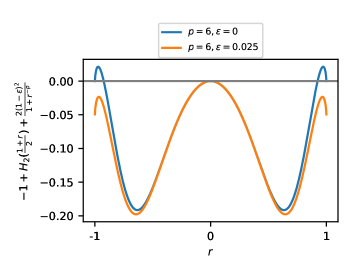
Figure 1: Example form of the function $\Lambda_{p,\epsilon}(r)$ analyzed in Lemma 12. For any $\epsilon>0$ it is possible to choose a $p$ large enough such that for $r\in\left[-1,1\right]$, $\Lambda_{p,\epsilon}(r)\leq 0$, with equality only at $r=0$.

Lemma 12.

For every $\epsilon>0$ there exists large enough $p$ such that the function

$$\Lambda_{p,\epsilon}(r)=\binom{n}{\frac{n+rn}{2}}\exp_{2}\left(-n+\frac{2(1-\epsilon)^{2}}{1+r^{-p}}n\right)$$ (65)

over the domain $r\in\left[-1,1\right]$ achieves its maximum at $r=0$ in the limit of large $n$.

Proof.

From Stirling’s approximation we have that

$$\binom{n}{\frac{n+rn}{2}}=\exp_{2}\left(\left(H_{2}\left(\frac{1+r}{2}\right)+o(1)\right)n\right),$$ (66)

where $H_{2}(p)=-p\log_{2}(p)-(1-p)\log_{2}(1-p)$ is the binary entropy function. Furthermore, the binomial coefficient is maximized when $r=0$ where

$${n\choose n/2}=(1+o(1))\sqrt{\frac{2}{\pi n}}.$$ (67)

Thus, we have that

$$\Lambda_{p,\epsilon}(r)=\exp_{2}\left(\left(H_{2}\left(\frac{1+r}{2}\right)+\frac{2(1-\epsilon)^{2}}{1+r^{-p}}-1+o(1)\right)n\right),\quad\quad\Lambda_{p,\epsilon}(0)=\exp_{2}(o(n)).$$ (68)

Let us denote $g(r,\epsilon,p)=H_{2}\left(\frac{1+r}{2}\right)+\frac{2(1-\epsilon)^{2}}{1+r^{-p}}-1$. The form of this function is shown as an example in Figure 1. The function $g$ is even for $p$ even. For $p$ odd, the function is negative for $r<0$ so we need only consider the range $r\in(0,1]$. Note that $H_{2}\left(\frac{1+r}{2}\right)$ is concave and equal to $0$ at the endpoints $r\in\{-1,+1\}$. In the range $r=(0,1]$, the function $\frac{2(1-\epsilon)^{2}}{1+r^{-p}}$ is decreasing with $p$. Sending $p\to\infty$, it is clear that for any $\epsilon>0$, there exists $p$ large enough so that the contribution from $\frac{2(1-\epsilon)^{2}}{1+r^{-p}}$ is decaying fast enough so that the function $g(r,\epsilon,p)<0$ in its tail.

We can calculate the scaling of the required $\epsilon$ with $p$. Using an upper-bound on $H_{2}\left(\frac{1+r}{2}\right)$ in the interval $r\in\left(0,1\right]$:

$$H_{2}\left(\frac{1+r}{2}\right)+\frac{2(1-\epsilon)^{2}}{1+r^{-p}}-1\leq\sqrt{1-r^{2}}+\frac{2(1-\epsilon)^{2}}{1+r^{-p}}-1.$$ (69)

It therefore suffices to choose $\epsilon$ such that:

$$\left(1-\epsilon\right)^{2}<\frac{1}{2}\left(1-\sqrt{1-r^{2}}\right)\left(1+r^{-p}\right)$$ (70)

for all $r\in\left(0,1\right]$. By taking a derivative we find that the right-hand side is minimized over $r$ on the interval $r\in\left(0,1\right]$ when:

$$r^{2}\left(1+r^{p}\right)+p\left(1-r^{2}-\sqrt{1-r^{2}}\right)=0.$$ (71)

It is straightforward to check that

$$r=1-\frac{2}{p^{2}}+O\left(\frac{1}{p^{3}}\right)$$ (72)

solves Equation 71 up to terms of the order $O\left(\frac{1}{p^{2}}\right)$. To leading nontrivial order in $p$, then,

$$\left(1-\epsilon\right)^{2}<\frac{1}{2}\left(1-\frac{2}{p}+O\left(\frac{1}{p^{2}}\right)\right)2=1-\frac{2}{p}+O\left(\frac{1}{p^{2}}\right)$$ (73)

suffices. That is, one can take any $p$ such that

$$\epsilon>\frac{1}{p}+O\left(\frac{1}{p^{2}}\right).$$ (74)

∎

4.3 Alternative derivation from concentration properties

For an alternative derivation of the maximum limiting energy of the classical $p$-spin model, one can also proceed via proof by contradiction in relation to the concentration properties of the model. Here, we will first show that $\mathbb{P}\left(\max_{\tau}H^{c}_{n,p}(\tau)\geq C_{\epsilon}n\right)\geq O(1/n)$ and then boost this to probability $1-o(1)$ by showing that if $\mathbb{E}\max_{\tau}H^{c}_{n,p}(\tau)<C_{2\epsilon}n$, it would contradict the concentration properties stated in Proposition 8. This strategy is due to Frieze [Fri90].

We start from Equation 60 copied below:

$$\begin{split}\frac{\mathbb{E}\left[N_{\epsilon}^{2}\right]}{\mathbb{E}\left[N_{\epsilon}\right]^{2}}&\leq\left(1+o\left(1\right)\right)\sum_{r=-\frac{n}{2}}^{\frac{n}{2}}\binom{n}{\frac{n+2r}{2}}\frac{\exp_{2}\left(-n+\frac{2(1-\epsilon)^{2}}{1+(\frac{n}{2r})^{p}}n\right)}{\left(1-\left(\frac{2r}{n}\right)^{2p}\right)^{-1/2}\left(1-\left(\frac{2r}{n}\right)^{p}\right)}.\end{split}$$ (75)

We split the sum above into two sums, the first corresponding to the case $|r|>(1-1/p)n$ and the second corresponding to the complementary case $|r|\leq(1-1/p)n$. In the former case we obtain using $|r|\leq n-1$ namely $|r/n|\leq 1-1/n$, that

$$\sum_{r:|r|>(1-1/p)n}\binom{n}{\frac{n+r}{2}}\frac{\exp_{2}\left(-n+\frac{2(1-\epsilon)^{2}}{1+(\frac{n}{r})^{p}}n\right)}{\left(1-\left(\frac{r}{n}\right)^{2p}\right)^{-1/2}\left(1-\left(\frac{r}{n}\right)^{p}\right)}$$ (76)

$$\leq n^{O(1)}\max_{r:|r|\geq(1-1/p)n}\exp_{2}\left(-n+\frac{2(1-\epsilon)^{2}}{1+(\frac{n}{r})^{p}}n\right)\sum_{r:|r|>(1-1/p)n}\binom{n}{\frac{n+r}{2}}.$$

By Stirling’s approximation

$${n\choose n+r/2} =\exp_{2}\left(nH_{2}(1/2+r/2)+\log n\right)$$ (77)

$$\leq\exp_{2}\left(nH_{2}(1-1/(2p))+\log n\right),$$ (78)

where $H_{2}(s)=-s\log s-(1-s)\log s$ is the binary entropy function.

On the other hand

$$-n+\frac{2(1-\epsilon)^{2}}{1+(\frac{n}{r})^{p}}n \leq-n+(1-\epsilon)^{2}n$$ (79)

$$\leq-2\epsilon(1-\epsilon)n,$$ (80)

since this expression is monotone in $r$. For any fixed $\epsilon>0$ we find large enough $p$ so that $H_{2}(1-1/(2p))<2\epsilon(1-\epsilon)$ and, as a result, the expression under $\exp_{2}(\cdot)$ is at most $-\Omega(n)$. Since the number of terms in the sum is at most linear in $n$, the sum in Equation 76—namely the contribution from the case $|r|\geq(1-1/p)n$—vanishes as $n\to\infty$.

We now turn to the second case when $|r|\leq(1-1/p)n$. In this case, $|r/n|\leq 1-1/p\leq\mathrm{e}^{-1/p}$ and thus $|r/n|^{p}\leq 1/\mathrm{e}$ so we obtain a bound:

$$\sum_{r:|r|\leq(1-1/p)n}\binom{n}{\frac{n+r}{2}}\frac{\exp_{2}\left(-n+\frac{2(1-\epsilon)^{2}}{1+(\frac{n}{r})^{p}}n\right)}{\left(1-\left(\frac{r}{n}\right)^{2p}\right)^{-1/2}\left(1-\left(\frac{r}{n}\right)^{p}\right)}$$ (81)

$$\leq O(1)\sum_{r:|r|\leq(1-1/p)n}\binom{n}{\frac{n+r}{2}}\exp_{2}\left(-n+\frac{2(1-\epsilon)^{2}}{1+(\frac{n}{r})^{p}}n\right)$$ (82)

$$=O(1)\sum_{r:|r|\leq(1-1/p)n}\exp_{2}\left(nH_{2}(1/2+r/2)+\log n\right)\exp_{2}\left(-n+\frac{2(1-\epsilon)^{2}}{1+(\frac{n}{r})^{p}}n\right)$$ (83)

where we used Stirling’s approximation again. Applying Lemma 12, giving $\Lambda(0)=O(1/\sqrt{n})=o(1)$, we obtain an upper bound $O(1/\sqrt{n})|\{r:|r|\leq(1-1/p)n\}|=O(n)$.

In conclusion $\frac{\mathbb{E}\left[N_{\epsilon}^{2}\right]}{\mathbb{E}\left[N_{\epsilon}\right]^{2}}=O(n)$. Applying the Paley–Zygmund inequality we conclude that

$$\mathbb{P}\left(\max_{\tau}H^{c}_{n,p}(\tau)\geq C_{\epsilon}n\right)\geq O(1/n).$$ (84)

We now use a standard argument based on concentration property stating that in fact this lower bound on probability can be boosted to $1-o(1)$. First we claim that

$$\mathbb{E}\left[\max_{\tau}H^{c}_{n,p}(\tau)\right]\geq C_{2\epsilon}n$$ (85)

for every $\epsilon>0$ and every sufficiently large $p$. Indeed, assume this is not the case. Then by the concentration bound given in Proposition 8 we obtain that

$$\mathbb{P}\left(\max_{\tau}H^{c}_{n,p}(\tau)\geq C_{\epsilon}n\right) \leq\mathbb{P}\left(\max_{\tau}H^{c}_{n,p}(\tau)-\mathbb{E}\left[\max_{\tau}H^{c}_{n,p}(\tau)\right]\geq C_{\epsilon}n-C_{2\epsilon n}n\right)$$ (86)

$$\leq 2\exp\left(-O\left({\left(C_{\epsilon}-C_{2\epsilon}\right)^{2}n}\right)\right).$$ (87)

Since $C_{\epsilon}>C_{2\epsilon}$, we obtain a contradiction with Equation 84. Thus Equation 85 holds. Applying concentration bound again we obtain that $\max_{\tau}H^{c}_{n,p}(\tau)\geq C_{3\epsilon}n$ with probability at least $1-\exp(-\Omega(n))$, completing the proof.

5 Expected maximum eigenvalue in the quantum $p$-spin model: Proof of Theorem 2

5.1 Upper bound on the expected maximum eigenvalue

In this subsection we obtain an upper bound on $E^{*}_{n}(p)=\mathbb{E}[\lambda_{max}(H_{n,p})/\sqrt{n}]$ again by resorting to the trace method. Our goal is to prove a bound

$$\mathbb{E}[\lambda_{max}(H_{n,p})/\sqrt{n}]\leq\sqrt{2\log 6}+o(1).$$ (88)

We note that this bound holds for any fixed $p\geq 2$. The asymptotics $p\to\infty$ is only being used to obtain a matching lower bound.

Fix $\beta>0$. We have that

$$\mathbb{E}[\lambda_{max}(H_{n,p})/\sqrt{n}]\leq{1\over\beta n}\mathbb{E}\left[\log\Tr\left(\exp\left(\beta\sqrt{n}H_{n,p}\right)\right)\right]\leq{1\over\beta n}\log\mathbb{E}\left[\Tr\left(\exp\left(\beta\sqrt{n}H_{n,p}\right)\right)\right],$$ (89)

and the bound will be obtained via a more tractable right-hand side expression corresponding to the annealed average. It will be convenient to switch from the Gaussian disorder $\alpha\in\mathcal{N}(0,1)$ to the Rademacher disorder $\alpha=\pm 1$ with probability $1/2$ each for our upper bound derivation. This is justified by Theorem 6. It is straightforward to see that the condition in Equation 18 is verified in particular.

Consider the first moment of the partition function:

$$\mathbb{E}\left[\Tr\left(\exp\left(\beta\sqrt{n}H_{n,p}\right)\right)\right]=\sum\limits_{m=0}^{\infty}\frac{\left(\beta\sqrt{n}\right)^{m}}{\binom{n}{p}^{\frac{m}{2}}m!}\sum\limits_{\begin{subarray}{c}\bm{\overline{i}_{1}},\ldots,\bm{\overline{i}_{m}}\\ \bm{\overline{a}_{1}},\ldots,\bm{\overline{a}_{m}}\end{subarray}}\mathbb{E}\left[\alpha\left[\bm{\overline{i}_{1}};\bm{\overline{a}_{1}}\right]\ldots\alpha\left[\bm{\overline{i}_{m}};\bm{\overline{a}_{m}}\right]\right]\Tr\left(P_{\bm{\overline{i}_{1}}}^{\bm{\overline{a}_{1}}}\ldots P_{\bm{\overline{i}_{m}}}^{\bm{\overline{a}_{m}}}\right).$$ (90)

Note that $\Tr\left(P_{\bm{\overline{i}_{\pi_{1}}}}^{\bm{\overline{a}_{\pi_{1}}}}\ldots P_{\bm{\overline{i}_{\pi_{2r}}}}^{\bm{\overline{a}_{\pi_{2r}}}}\right)$ contributes to the final sum only when all Pauli observables in the trace mutually commute. To see this, assume two neighboring Paulis in the sum $P_{\bm{\overline{i}_{\pi_{\ell}}}}^{\bm{\overline{a}_{\pi_{\ell}}}},P_{\bm{\overline{i}_{\pi_{\ell+1}}}}^{\bm{\overline{a}_{\pi_{\ell+1}}}}$ anticommute. We then have that:

$$\Tr\left(P_{\bm{\overline{i}_{\pi_{1}}}}^{\bm{\overline{a}_{\pi_{1}}}}\ldots P_{\bm{\overline{i}_{\pi_{\ell}}}}^{\bm{\overline{a}_{\pi_{\ell}}}}P_{\bm{\overline{i}_{\pi_{\ell+1}}}}^{\bm{\overline{a}_{\pi_{\ell+1}}}}\ldots P_{\bm{\overline{i}_{\pi_{2r}}}}^{\bm{\overline{a}_{\pi_{2r}}}}\right)+\Tr\left(P_{\bm{\overline{i}_{\pi_{1}}}}^{\bm{\overline{a}_{\pi_{1}}}}\ldots P_{\bm{\overline{i}_{\pi_{\ell+1}}}}^{\bm{\overline{a}_{\pi_{\ell+1}}}}P_{\bm{\overline{i}_{\pi_{\ell}}}}^{\bm{\overline{a}_{\pi_{\ell}}}}\ldots P_{\bm{\overline{i}_{\pi_{2r}}}}^{\bm{\overline{a}_{\pi_{2r}}}}\right)=0.$$ (91)

Thus since the expectation parts contribute the same value under permutations, the terms associated with $\pi$ and $\begin{pmatrix}\ell&\ell+1\end{pmatrix}\pi$ cancel. This is also true when Pauli operators $P_{\bm{\overline{i}_{\pi_{\ell}}}}^{\bm{\overline{a}_{\pi_{\ell}}}},P_{\bm{\overline{i}_{\pi_{\ell+g}}}}^{\bm{\overline{a}_{\pi_{\ell+g}}}}$ in the sum anticommute, with $P_{\bm{\overline{i}_{\pi_{\ell}}}}^{\bm{\overline{a}_{\pi_{\ell}}}}$ commuting with all Pauli operators between them in the trace. We once again have that the term associated with $\pi$ and $\begin{pmatrix}\ell&\ell+g\end{pmatrix}\pi$ cancel. By choosing nearest anticommuting pairs of Pauli operators, then, one can uniquely match permutations in a way such that all contributions cancel. Therefore from now one we may restrict the sum above to superindices $\bar{\bm{i}}_{1},\ldots,\bar{\bm{i}}_{m}$ which mutually commute. This is a crucial observation for the derivation of our upper bound part.

Next we note that since the Rademacher disorder is symmetric, the expectation $\mathbb{E}\left[\alpha\left[\bm{\overline{i}_{1}};\bm{\overline{a}_{1}}\right]\ldots\alpha\left[\bm{\overline{i}_{m}};\bm{\overline{a}_{m}}\right]\right]$ is non-zero only when each pair $[\bar{\bm{i}},\bar{\bm{a}}]$ appears in the product an even number of times. In this case the expectation is $1$ (this is where working with Rademacher disorder is convenient). Thus we rewrite Equation 90 as

$$\mathbb{E}\left[\Tr\left(\exp\left(\beta\sqrt{n}H_{n,p}\right)\right)\right]=\sum\limits_{m=0}^{\infty}\frac{\left(\beta\sqrt{n}\right)^{m}}{\binom{n}{p}^{\frac{m}{2}}m!}\sum\limits_{\begin{subarray}{c}\bm{\overline{i}_{1}},\ldots,\bm{\overline{i}_{m}}\\ \bm{\overline{a}_{1}},\ldots,\bm{\overline{a}_{m}}\end{subarray}}\Tr\left(P_{\bm{\overline{i}_{1}}}^{\bm{\overline{a}_{1}}}\ldots P_{\bm{\overline{i}_{m}}}^{\bm{\overline{a}_{m}}}\right)$$ (92)

where the sum is restricted to $m$-tuples $\left(\left[\bm{\overline{i}_{1}};\bm{\overline{a}_{1}}\right],\ldots,\left[\bm{\overline{i}_{m}};\bm{\overline{a}_{m}}\right]\right)$ such that (a) each term $\left[\bm{\overline{i}};\bm{\overline{a}}\right]$ appears an even number of times in the $m$-tuple and (b) all ${m\choose 2}$ pairs of terms commute. We denote the set of such $m$-tuples by $\mathcal{S}_{m,\rm e,com}$. As the trace gives $2^{n}$ when all Pauli operators in the trace mutually commute, we therefore have that:

$$\mathbb{E}\left[\Tr\left(\exp\left(\beta\sqrt{n}H_{n,p}\right)\right)\right]=2^{n}\sum\limits_{m=0}^{\infty}\frac{\left(\beta\sqrt{n}\right)^{m}}{\binom{n}{p}^{\frac{m}{2}}m!}|\mathcal{S}_{m,\rm e,com}|.$$ (93)

Next we establish that the contribution from superlinear terms $m=\omega(n)$ in the sum above is negligible.

Lemma 13.

For every $\beta,p$ and $\epsilon>0$ there exists $C=C(\beta,p,\epsilon)$ such that the sum in Equation 93 restricted to the range where $m\geq Cn$ is at most $\exp\left(-\epsilon n\right)$.

Proof.

For the purposes of the proof the commutation requirement will be ignored. Recall that for each $m$-tuple in $\mathcal{S}_{m,\rm e,com}$, each pair $[\bar{\bm{i}};\bar{\bm{a}}]$ appears in this $m$-tuple an even number of times. Thus the total number $r$ of distinct pairs $[\bar{\bm{i}},\bar{\bm{a}}]$ in each $m$-tuple is at most $m/2$. Note that the total number of distinct pairs is $3^{p}{n\choose p}$. Let $m_{0}=\min(m/2,3^{p}{n\choose p})$ which is an upper bound on the number of distinct pairs in each $m$-tuple. Over all $r\leq m_{0}$ the number of choices for $r$-sets of such distinct pairs is then at most

$$\sum_{r\leq m_{0}}{3^{p}{n\choose p}\choose r}\leq m_{0}{\left(3^{p}{n\choose p}\right)^{m_{0}}\over m_{0}!}$$ (94)

where monotonicity in $r\leq m_{0}$ was used. Let $m_{1},\ldots,m_{r}$ denote the multiplicities of each distinct pair among the sequence of $m$ pairs. The total number of choices of $m_{1},\ldots,m_{r}$ is ${m-1\choose r-1}\leq 2^{m}$. An upper bound on the number of permutations for each $m$-tuple is $m!$. Thus we obtain

$$2^{n}\sum\limits_{m\geq Cn}\frac{\left(\beta\sqrt{n}\right)^{m}}{\binom{n}{p}^{\frac{m}{2}}m!}|\mathcal{S}_{m,\rm e,com}| \leq 2^{n}\sum\limits_{m\geq Cn}\frac{\left(\beta\sqrt{n}\right)^{m}}{\binom{n}{p}^{\frac{m}{2}}m!}m_{0}{\left(3^{p}{n\choose p}\right)^{m_{0}}\over m_{0}!}m!2^{m}$$ (95)

$$=2^{n}\sum\limits_{m\geq Cn}\frac{\left(\beta\sqrt{n}\right)^{m}}{\binom{n}{p}^{\frac{m}{2}}}{\left(3^{p}{n\choose p}\right)^{m_{0}}\over(m_{0}-1)!}2^{m}.$$ (96)

We split the sum into two cases. First consider the range $m\geq 2(3^{p}){n\choose p}$. In this case $m_{0}=3^{p}{n\choose p}$ and our range is $m\geq 2m_{0}$. We have

$$\sum_{m\geq 2m_{0}}{\left(\beta\sqrt{n}\right)^{m}\over\binom{n}{p}^{m\over 2}}2^{m}=(1+o(1))\left({2\beta\sqrt{n}\over{n\choose p}^{1\over 2}}\right)^{2m_{0}}.$$ (97)

We thus obtain a bound

$$2^{n}\sum\limits_{m\geq 2(3^{p}){n\choose p}}\frac{\left(\beta\sqrt{n}\right)^{m}}{\binom{n}{p}^{\frac{m}{2}}m!}|\mathcal{S}_{m,\rm e,com}|\leq 2^{n}(1+o(1)){\left(2\beta(3^{p\over 2})\sqrt{n}\right)^{2m_{0}}\over(m_{0}-1)!}.$$ (98)

Since $m_{0}=\Theta(n^{p})$ with $p\geq 2$, the value above is bounded as $2^{n}2^{-\Omega(m_{0})}=2^{-\Omega(n^{p})}$.

Next we consider the range $Cn\leq m\leq 2(3^{p}){n\choose p}$. In this case $m_{0}=m/2$. We obtain a sum

$$2^{n}\sum_{Cn\leq m\leq 2(3^{p}){n\choose p}}\frac{\left(\beta\sqrt{n}\right)^{m}}{\binom{n}{p}^{\frac{m}{2}}}{\left(3^{p}{n\choose p}\right)^{m\over 2}\over(m/2-1)!}2^{m}=2^{n}\sum_{Cn\leq m\leq 2(3^{p}){n\choose p}}{\left(4\beta^{2}n3^{p}\right)^{m\over 2}\over(m/2-1)!}.$$ (99)

This sum is of the form $\sum_{r\geq Cn}(\lambda n)^{r}/r!$ for some constant $\lambda$. This sum is at most $\exp(-\epsilon n)$ for sufficiently large $C$. ∎

Applying Lemma 13 to Equation 93 we obtain

$$\mathbb{E}\left[\Tr\left(\exp\left(\beta\sqrt{n}H_{n,p}\right)\right)\right]=2^{n}\sum\limits_{m\leq Cn}\frac{\left(\beta\sqrt{n}\right)^{m}}{\binom{n}{p}^{\frac{m}{2}}m!}|\mathcal{S}_{m,\rm e,com}|+\exp(-\Omega(n)).$$ (100)

We proceed to obtaining upper bounds on $|\mathcal{S}_{m,\rm e,com}|$.

Lemma 14.

Suppose $m=O(n)$. For all large enough $n$ the number of ordered $m$-tuples $\bar{\bm{i}}_{1},\ldots,\bar{\bm{i}}_{m}$ of size-$p$ subsets of $[n]$ such that each subset appears an even number of times is at most

$$2^{o(n)}{n\choose p}^{m/2}{m!\over(m/2)!2^{m/2}}.$$ (101)

Proof.

With some abuse of notation, we denote the set of distinct $p$-sets appearing in the $m$-tuple by $\bar{\bm{i}}_{1},\ldots,\bar{\bm{i}}_{r}$ and the corresponding multiplicities by $m_{1},\ldots,m_{r}$ so that $m_{j}\geq 2$ and $\sum_{1\leq j\leq r}m_{j}=m$. The number of choices for $r$ such distinct sets is

$${{n\choose p}\choose r}\leq{{n\choose p}^{r}\over r!}.$$ (102)

For each $(m_{1},\ldots,m_{r})$ multi-set of such $r$ $p$-sets, the number of distinct orderings of them is

$${m!\over\prod_{1\leq j\leq r}m_{j}!}.$$ (103)

We obtain an upper bound:

$$\sum_{r,m_{1},\ldots,m_{r}}{{n\choose p}^{r}\over r!}{m!\over\prod_{j}m_{j}!}.$$ (104)

We consider two cases. First we consider the case when $r\leq m/2-n/\sqrt{\log n}$. The total number of terms in the sum $\sum_{r,m_{1},\ldots,m_{r}}$ is $2^{O(n)}$. Ignoring the $m_{j}!$ terms, we obtain an upper bound:

$$2^{O(n)}m!{{n\choose p}^{r}\over r!}.$$ (105)

Since $r=O(n)$ and ${n\choose p}=\Theta(n^{p})$, with $p\geq 2$, we have $r/{n\choose p}=O(1/n^{p-1})$ and therefore

$${{n\choose p}^{r}\over r!}=n^{-\Omega(n/\sqrt{\log n})}{{n\choose p}^{m/2}\over(m/2)!}=2^{-\Omega(n\sqrt{\log n})}{{n\choose p}^{m/2}\over(m/2)!}.$$ (106)

Thus in the case $r\leq m/2-n/\sqrt{\log n}$ the contribution is at most superexponential factor $2^{-\Omega(n\sqrt{\log n})}$ smaller than Equation 101.

Next we consider the case when $r\geq m/2-n/\sqrt{\log n}$. Let $r_{0}$ be the number of terms $m_{j}=2$. Then

$$m\geq 2r_{0}+4(r-r_{0})=2r+2(r-r_{0})\geq m-2n/\sqrt{\log n}+2(r-r_{0}),$$ (107)

implying $r_{0}\geq r-n/\sqrt{\log n}\geq m/2-2n/\sqrt{\log n}$. We claim that the number of choices for $r,m_{1},\ldots,m_{r}$ in this case is $2^{o(n)}$. To see this we have ${r\choose r_{0}}=2^{o(n)}$ choices for the location of terms $m_{j}$ with $m_{j}\geq 4$. For each fixed set of locations (assuming these are $1,\ldots,r-r_{0}$ for convenience), the number of configurations of the form $m_{1}+\cdots+m_{r-r_{0}}=m-2r_{0}=O(n/\sqrt{\log n})$ is $2^{O(n/\sqrt{\log n})}=2^{o(n)}$. Using this expression in Equation 104 we thus have the upper bound:

$$\begin{split}2^{o(n)}{{n\choose p}^{r}\over r!}{m!\over 2^{r_{0}}}&\leq 2^{o(n)}{{n\choose p}^{r}\over r!}{m!\over 2^{m/2}}2^{O(n/\sqrt{\log n})}\\ &=2^{o(n)}{{n\choose p}^{r}\over r!}{m!\over 2^{m/2}}.\end{split}$$ (108)

Finally, since ${{n\choose p}^{r}\over r!}$ is increasing as a function of $r$ when $r=O(n)$ and since $r\leq m/2$, we obtain the claimed upper bound. ∎

We now show that when $r=O(n)$ size-$p$ sets are chosen uniformly at random independently, the number of pairs of superindices $\bar{\bm{i}}$ which overlap in more than one qubit is rare. Given $r$ subsets $\bar{\bm{i}}_{1},\ldots\bar{\bm{i}}_{r}\subset[n]$, let $\mathcal{I}_{2}=\mathcal{I}_{2}(\bar{\bm{i}}_{1},\ldots\bar{\bm{i}}_{r})=\{(\bar{\bm{i}}_{\ell},\bar{\bm{i}}_{s}),|\bar{\bm{i}}_{\ell}\cap\bar{\bm{i}}_{s}|\geq 2,1\leq\ell<s\leq r\}$. Namely, $\mathcal{I}_{2}$ is the set of all pairs of these sets intersecting in at least 2 qubits. Let $\mathcal{V}=\mathcal{V}(\bar{\bm{i}}_{1},\ldots\bar{\bm{i}}_{r})$ be the set of sets which span $\mathcal{I}_{2}$. Namely, $\mathcal{V}=\{\ell\in[r]:\exists s\in[r]~{}(\bar{\bm{i}}_{\ell},\bar{\bm{i}}_{s})\in\mathcal{I}_{2}\}$.

Lemma 15.

Suppose $r=O(n)$ cardinality-$p$ subsets $\bar{\bm{i}}_{1},\ldots,\bar{\bm{i}}_{r}$ of $[n]$ are chosen uniformly at random independently from the set of all ${n\choose p}$ subsets. Then

$$\mathbb{P}\left(|\mathcal{V}|\geq n/\sqrt{\log n}\right)=\exp\left(-\Omega(n\sqrt{\log n})\right).$$ (109)

Namely, the number of superindices spanned by pairs overlapping in at least two qubits is sublinear with overwhelming (super-exponentially close to unity) probability.

Proof.

We fix a subset $V\subset[r]$ and estimate the probability of the event $\mathcal{V}=V$. We create a graph $G$ on $V$ where two elements of $V$ are connected by an edge if the corresponding superindices intersect in at least two qubits. Then the event $\mathcal{V}=V$ implies the event that every node in the graph $G$ is connected to least one other node in the same graph. Let $E$ be the set of edges in $G$ so that $G$ is described as a pair $(V,E)$. Then $|E|=|\mathcal{I}_{2}|$.

Let $V=\{\bar{\bm{i}}_{\ell_{1}},\ldots,\bar{\bm{i}}_{\ell_{|V|}}\}$. Split the graph $G$ into connected components $G_{1},\ldots,G_{L},L\geq 1$ with node sets $V_{1},\ldots,V_{L}$, so that $\bigcup_{t}V_{t}=V$. In each component $G_{t},1\leq t\leq L$ identify a spanning tree $T_{t}$. We fix a realization of the sequence $T_{1},\ldots,T_{L}$ and compute the likelihood of this realization. We claim that the likelihood of $T_{t}$ being realized is at most $2^{O(|V_{t}|)}/n^{2\left(|V_{t}|-1\right)}$. For this purpose fix any root node $o_{t}\in T_{t}$ and consider the breadth-first exploration process starting from $o_{t}$. Each node in the exploration process is connected to some node explored earlier. The likelihood of this taking place is $O(1/n^{2})$. Here we use the fact that the likelihood that two superindices $\bar{\bm{i}}_{1},\bar{\bm{i}}_{2}$ chosen uniformly at random independently intersect in at least two qubits is $O(1/n^{2})$. Furthermore, these events are independent since each next node in the exploration process has not been considered earlier. Since $T_{t}$ contains exactly $|V_{t}|-1$ edges we obtain the claimed upper bound $2^{O(|V_{t}|)}/n^{2|V_{t}|-2}$. Across the trees the bound is

$$\prod_{1\leq t\leq L}{2^{O(|V_{t}|)}\over n^{2|V_{t}|-2}}={2^{O(|V|)}\over n^{2|V|-2L}}.$$ (110)

The number of spanning trees supported on a fixed set of $v$ nodes is $v^{v-2}$, and thus by union bound, we obtain that conditioned on the components being supported on sets $V_{1},\ldots,V_{L}$ the probability of at least one tree being realized in each component is at most

$${2^{O(|V|)}\over n^{2|V|-2L}}\prod_{t}|V_{t}|^{|V_{t}|-2}\leq{2^{O(|V|)}\over n^{2|V|-2L}}|V|^{\sum_{t}(|V_{t}|-2)}\leq{2^{O(|V|)}|V|^{|V|-2L}\over n^{2|V|-2L}}.$$ (111)

The number of partitions of $V$ into subsets $V_{1},\ldots,V_{L}$ is $2^{O(|V|)}$ which is absorbed by the bound above. Finally, the number of choices for $V$ is

$${r\choose|V|}\leq{r^{|V|}\over|V|!}=2^{O(|V|)}{n^{|V|}\over|V|!},$$ (112)

which leads to a bound

$$2^{O(|V|)}{|V|^{|V|-2L}\over|V|!n^{|V|-2L}}=2^{O(|V|)}{|V|^{-2L}\over n^{|V|-2L}}=2^{O(|V|)}{1\over n^{|V|}}\left({n\over|V|}\right)^{2L}\leq 2^{O(|V|)}{1\over n^{|V|}}\left({n\over|V|}\right)^{|V|}=2^{O(|V|)}{1\over|V|^{|V|}},$$ (113)

where Stirling’s approximation $v!=(1+o(1))v^{v}/e^{v}$ was used in the first equality, and $|V|\geq 2L$ was used in the inequality; this latter fact follows as every vertex is connected to at least one edge in the event $\mathcal{V}=V$. When $|V|\geq n/\sqrt{\log n}$ the required bound is obtained.

∎

Recall the definition of $\mathcal{V}(\bar{\bm{i}}_{1},\ldots,\bar{\bm{i}}_{r})$ of the set of size-$p$ sets defined for every fixed $r$-tuple $\bar{\bm{i}}_{1},\ldots,\bar{\bm{i}}_{r}$ of size-$p$ sets of qubits. Let $\mathcal{N}\subset[n]$ be the set of qubits spanned by subsets $\bar{\bm{i}}$ in $\mathcal{V}$. Let $\mathcal{N}_{0}$ be the set of qubits spanned by the remaining elements in the $r$-tuple. That is $\mathcal{N}_{0}=\left(\cup_{1\leq j\leq m}\bar{\bm{i}}_{j}\right)\setminus\mathcal{N}$. We now obtain an upper bound on $\mathcal{S}_{m,\rm e,com}$ in terms of the cardinalities of $\mathcal{N}_{0}$ and $\mathcal{V}$.

Fix any sequence of size-$p$ sets $\bar{\bm{i}}_{1},\ldots,\bar{\bm{i}}_{m}$ such that each element $\bar{\bm{i}}_{j}$ appears in this sequence an even number of times. Note that only such sequences can contribute to $\mathcal{S}_{m,\rm e,com}$. Let $\mathcal{A}_{m,\rm e,com}\left(\bar{\bm{i}}_{1},\ldots,\bar{\bm{i}}_{m}\right)\subset\{1,2,3\}^{m}$ be the set of all $m$-tuples $(\bar{\bm{a}}_{1},\ldots,\bar{\bm{a}}_{m})$ such that $\left(\left[\bm{\overline{i}_{1}};\bm{\overline{a}_{1}}\right],\ldots,\left[\bm{\overline{i}_{m}};\bm{\overline{a}_{m}}\right]\right)\in\mathcal{S}_{m,\rm e,com}$. We claim that

$$|\mathcal{A}_{m,\rm e,com}|\leq 3^{|\mathcal{N}_{0}|}3^{|\mathcal{V}|}\leq 3^{n}3^{|\mathcal{V}|},$$ (114)

where $\mathcal{N}_{0}=\mathcal{N}_{0}(\bar{\bm{i}}_{1},\ldots,\bar{\bm{i}}_{m})$ and $\mathcal{V}=\mathcal{V}(\bar{\bm{i}}_{1},\ldots,\bar{\bm{i}}_{m})$. The second inequality is immediate. To justify the first inequality, observe that if $\bar{\bm{i}}_{k_{1}},\bar{\bm{i}}_{k_{2}}\in\{\bar{\bm{i}}_{1},\ldots,\bar{\bm{i}}_{m}\}$ intersect in some qubit $i\in\mathcal{N}_{0}$, then they intersect only in one qubit in total, by the definition of $\mathcal{N}_{0}$. In this case $[\bar{\bm{i}}_{k_{1}};\bar{\bm{a}}_{k_{1}}],[\bar{\bm{i}}_{k_{2}};\bar{\bm{a}}_{k_{2}}]$ can commute only if the corresponding entries of $\bar{\bm{a}}_{k_{1}}$ and $\bar{\bm{a}}_{k_{2}}$ agree. In other words, there is only one of 3 choices of Pauli operators for each qubit in $\mathcal{N}_{0}$. We also have a trivial deterministic bound $|\mathcal{A}_{m,\rm e,com}|\leq 3^{m}$. Combining these bounds with Lemma 14 and Lemma 15 we obtain the following bound:

$$|\mathcal{S}_{m,\rm e,com}|\leq 2^{o(n)}{{n\choose p}^{m/2}m!\over(m/2)!2^{m/2}}3^{n}\left(3^{n/\sqrt{\log n}}+3^{m}\exp\left(-\Omega(n\sqrt{\log n}\right)\right)={{n\choose p}^{m/2}m!\over(m/2)!2^{m/2}}3^{n+o(n)}$$ (115)

when $m$ is even, where $m=O(n)$ was used in the equality part. We recall that that when $m$ is odd the set $\mathcal{S}_{m,\rm e,com}$ is empty. Applying this bound to Equation 100 we obtain

$$\begin{split}\mathbb{E}\left[\Tr\left(\exp\left(\beta\sqrt{n}H_{n,p}\right)\right)\right]&\leq 2^{n}\sum\limits_{m\textrm{ even},m\leq Cn}\frac{\left(\beta\sqrt{n}\right)^{m}}{\binom{n}{p}^{\frac{m}{2}}m!}{{n\choose p}^{m/2}m!\over(m/2)!2^{m/2}}3^{n+o(n)}\\ &=6^{n+o(n)}\sum\limits_{m\textrm{ even},m\leq Cn}{\left(\beta\sqrt{n}\right)^{m}\over(m/2)!2^{m/2}}\\ &\leq 6^{n+o(n)}\sum\limits_{m\textrm{ even},m\geq 0}{\left(\beta\sqrt{n}\right)^{m}\over(m/2)!2^{m/2}}\\ &=6^{n+o(n)}\sum\limits_{r\geq 0}{\left(\beta^{2}n\right)^{r}\over r!2^{r}}\\ &=6^{n+o(n)}\exp\left({\beta^{2}n\over 2}\right),\end{split}$$ (116)

where the $\exp(-\Omega(n))$ term is absorbed by the $o(n)$ in the exponent in the first inequality.

We are ready to complete the proof of Equation 88. Applying we obtain

$$\mathbb{E}[\lambda_{max}(H_{n,p})/\sqrt{n}]\leq\beta^{-1}\log 6+\beta/2+o(1).$$ (117)

Minimizing over $\beta$ we obtain $\beta=\sqrt{2\log 6}$ and an upper bound

$$\limsup_{n\to\infty}\mathbb{E}[\lambda_{max}(H_{n,p})/\sqrt{n}]\leq\sqrt{2\log 6},$$ (118)

completing the proof of Equation 88.

5.2 Matching lower bound in the large $p$ limit

We now compute a matching lower bound for large $p$. We achieve this by applying the second moment method to the number $N_{\epsilon}$ of Pauli-basis states $\ket{\bm{a},\bm{b}}\in\mathcal{S}^{n}_{\rm Pauli}$ (see Equation 12 for an introduction to this notation) above normalized energy threshold $(1-\epsilon)\sqrt{2\log 6}$ for some $\epsilon\geq 0$. Specifically,

$$N_{\epsilon}=\left|\left\{\ket{\bm{a},\bm{b}}\in\mathcal{S}^{n}_{\rm Pauli}:\sqrt{n}\bra{\bm{a},\bm{b}}H_{n,p}\ket{\bm{a},\bm{b}}\geq(1-\epsilon)\sqrt{2\log 6}n\right\}\right|.$$ (119)

To simplify notation we introduce the constant $C_{\epsilon}\coloneqq(1-\epsilon)\sqrt{2\log 6}$. We also normalize the quantum Hamiltonian as $\sqrt{n}H_{n,p}$ so that the variance (over the distribution of $\bm{\alpha}$) of the energy expectation for a product state is equal to $n$. The second moment method guarantees that $N_{\epsilon}>0$ via the Paley–Zygmund inequality:

$$\mathbb{P}\left[N_{\epsilon}>0\right]\geq\frac{\mathbb{E}[N_{\epsilon}]^{2}}{\mathbb{E}{[N_{\epsilon}^{2}]}}.$$ (120)

Since $\sqrt{n}\bra{\bm{a},\bm{b}}H_{n,p}\ket{\bm{a},\bm{b}}$ is Gaussian with mean zero and variance $n$ for any $\ket{\bm{a},\bm{b}}$, once again by the tail bound of Equation 55 the first moment is equal to

$$\begin{split}\mathbb{E}N_{\epsilon}&=\sum_{\bm{a}\in\left\{1,2,3\right\}^{n},\bm{b}\in\{-1,+1\}^{n}}\mathbb{P}[\sqrt{n}\bra{\bm{a},\bm{b}}H_{n,p}\ket{\bm{a},\bm{b}}\geq C_{\epsilon}n]\\ &=6^{n}\left(1-\Phi((1-\epsilon)\sqrt{2n\log 6}\sqrt{n})\right)\\ &=6^{n}\exp\left(-(1-\epsilon)^{2}\log(6)n\right)\frac{1}{\sqrt{2\pi}}\frac{1}{C_{\epsilon}\sqrt{n}+o(1)},\end{split}$$ (121)

where once again $\Phi$ is the cumulative distribution function of the standard normal distribution. For the second moment, we recall from Lemma 7 that the covariance of two different configurations is equal to:

$$\mathbb{E}\left[\bra{\bm{a},\bm{b}}H_{n,p}\ket{\bm{a},\bm{b}}\bra{\bm{\tilde{a}},\bm{\tilde{b}}}H_{n,p}\ket{\bm{\tilde{a}},\bm{\tilde{b}}}\right]=\frac{1}{\binom{n}{p}}\sum_{\bar{\bm{i}}\in\mathcal{I}_{p}^{n}:\bar{\bm{i}}\subseteq\Delta\left(\bm{a},\bm{\tilde{a}}\right)}\prod_{k=1}^{p}b_{i_{k}}\tilde{b}_{i_{k}}.$$ (122)

For simplicity, we will however consider an equivalent expression (up to $O\left(1/n\right)$ corrections):

$$\mathbb{E}\left[\bra{\bm{a},\bm{b}}H_{n,p}\ket{\bm{a},\bm{b}}\bra{\bm{\tilde{a}},\bm{\tilde{b}}}H_{n,p}\ket{\bm{\tilde{a}},\bm{\tilde{b}}}\right]=\left(\frac{1}{n}\sum_{i\in\Delta\left(\bm{a},\bm{\tilde{a}}\right)}b_{i}\tilde{b}_{i}\right)^{p}+O\left(\frac{1}{n}\right).$$ (123)

This follows as

$$\begin{split}\left|\left(\frac{1}{n}\sum_{i\in\Delta\left(\bm{a},\bm{\tilde{a}}\right)}b_{i}\tilde{b}_{i}\right)^{p}-\frac{p!{n\choose p}}{n^{p}}\frac{1}{{n\choose p}}\sum_{\begin{subarray}{c}i_{1}<\cdots<i_{p}\\ i_{1},\dots,i_{p}\in\Delta\left(\bm{a},\bm{\tilde{a}}\right)\end{subarray}}\prod_{k=1}^{p}b_{i_{k}}\tilde{b}_{i_{k}}\right|\leq\frac{n^{p}-p!{n\choose p}}{n^{p}}=O(1/n).\end{split}$$ (124)

We will use the shorthand

$$R\left(\bm{a},\bm{b},\bm{\tilde{a}},\bm{\tilde{b}}\right)\coloneqq\mathbb{E}\left[\bra{\bm{a},\bm{b}}H_{n,p}\ket{\bm{a},\bm{b}}\bra{\bm{\tilde{a}},\bm{\tilde{b}}}H_{n,p}\ket{\bm{\tilde{a}},\bm{\tilde{b}}}\right]$$ (125)

for this covariance in the following.

The joint probability is

$$\begin{split}\mathbb{P}&\left[\sqrt{n}\langle\bm{a},\bm{b}|H_{n,p}|\bm{a},\bm{b}\rangle\geq C_{\epsilon}n\cap\sqrt{n}\langle\bm{\tilde{a}},\bm{\tilde{b}}|H_{n,p}|\bm{\tilde{a}},\bm{\tilde{b}}\rangle\geq C_{\epsilon}n\right]\\ &\leq\mathbb{P}\left[\sqrt{n}\langle\bm{a},\bm{b}|H_{n,p}|\bm{a},\bm{b}\rangle\geq C_{\epsilon}n\right]\mathbb{P}\left[\sqrt{n}\langle\bm{\tilde{a}},\bm{\tilde{b}}|H_{n,p}|\bm{\tilde{a}},\bm{\tilde{b}}\rangle\geq C_{\epsilon}n\;|\;\sqrt{n}\langle\bm{a},\bm{b}|H_{n,p}|\bm{a},\bm{b}\rangle=C_{\epsilon}n\right]\\ &=\left[1-\Phi(C_{\epsilon}\sqrt{n})\right]\left[1-\Phi\left(C_{\epsilon}\left(1-R(\bm{a},\bm{b},\bm{\tilde{a}},\bm{\tilde{b}})^{2p}\right)^{-1/2}\left(1-R(\bm{a},\bm{b},\bm{\tilde{a}},\bm{\tilde{b}})^{p}\right)\sqrt{n}\right)\right].\end{split}$$ (126)

In the second line above, we use the monotonicity of the conditional CDF of the Gaussian for the inequality since the conditional CDF is minimized when conditioned on the smallest value possible.

We will now compute the second moment by changing a sum over configurations $\bm{a},\bm{\tilde{a}},\bm{b},\bm{\tilde{b}}$ to a sum over:

1. $\Delta$, how many indices $i$ on which $a_{i}=\tilde{a}_{i}$—namely, the cardinality of the set $\Delta\left(\bm{a},\bm{\tilde{a}}\right)$;

2. $\gamma$, how many indices $i$ on which $a_{i}\equiv\tilde{a}_{i}-1\pmod{3}$;

3. $2r\in[-\Delta,\Delta]$ , the inner product of $\bm{b}$ and $\bm{\tilde{b}}$ when restricted to indices $i\in\Delta\left(\bm{a},\bm{\tilde{a}}\right)$ on which $a_{i}=\tilde{a}_{i}$; the factor of $2$ arises from possible overlaps only differing by even numbers.

In this representation,

$$R\left(\bm{a},\bm{b},\bm{\tilde{a}},\bm{\tilde{b}}\right)=\left(\frac{2r}{n}\right)^{p}.$$ (127)

Given $\bm{a},\bm{b}$, then, the number of configurations $\bm{\tilde{a}},\bm{\tilde{b}}$ at a given $\Delta,\gamma,r$ is

$$\binom{n}{\Delta,\gamma,n-\Delta-\gamma}\binom{\Delta}{\frac{\Delta+2r}{2}}2^{n-\Delta}.$$ (128)

The first term (multinomial coefficient) is the number of ways of choosing the $\bm{\tilde{a}}$, the second term is the number of ways to get $2r$, and the third term is the number of configurations for the Pauli bases outside the set $\Delta\left(\bm{a},\bm{\tilde{a}}\right)$. From the above, we can calculate the second moment as

$$\begin{split}\mathbb{E}[N_{\epsilon}^{2}]&=\sum_{\bm{a},\bm{\tilde{a}}\in\left\{1,2,3\right\}^{n},\bm{b},\bm{\tilde{b}}\in\{-1,+1\}^{n}}\mathbb{P}\left[\sqrt{n}\langle\bm{a},\bm{b}|H_{n,p}|\bm{a},\bm{b}\rangle\geq C_{\epsilon}n\cap\sqrt{n}\langle\bm{\tilde{a}},\bm{\tilde{b}}|H_{n,p}|\bm{\tilde{a}},\bm{\tilde{b}}\rangle\geq C_{\epsilon}n\right]\\ &\leq\sum_{\Delta=0}^{n}\sum_{\gamma=0}^{n-\Delta}\sum_{r=-\frac{\Delta}{2}+\delta_{\Delta,n}}^{\frac{\Delta}{2}-\delta_{\Delta,n}}\binom{n}{\Delta,\gamma,n-\Delta-\gamma}\binom{\Delta}{\frac{\Delta+2r}{2}}2^{n-\Delta}\frac{1}{2\pi}\frac{\exp_{6}(n(2\epsilon-\epsilon^{2}))\exp_{6}\left(-(1-\epsilon)^{2}\left(\frac{1-(\frac{2r}{n})^{p}}{1+(\frac{2r}{n})^{p}}\right)n\right)}{C_{\epsilon}^{2}\left(1-\left(\frac{2r}{n}\right)^{2p}\right)^{-1/2}\left(1-\left(\frac{2r}{n}\right)^{p}\right)n+o(\sqrt{n})}+2\mathbb{E}[N_{\epsilon}],\end{split}$$ (129)

where we have used the notation $\exp_{6}\left(x\right)=6^{x}$ and $\delta_{\Delta,n}=1$ iff $\Delta=n$.

Then, taking the ratio and applying Equation 121:

$$\begin{split}\frac{\mathbb{E}\left[N_{\epsilon}^{2}\right]}{\mathbb{E}\left[N_{\epsilon}\right]^{2}}&\leq\left(1+o\left(1\right)\right)\sum_{\Delta=0}^{n}\sum_{\gamma=0}^{n-\Delta}\sum_{r=-\frac{\Delta}{2}+\delta_{\Delta,n}}^{\frac{\Delta}{2}-\delta_{\Delta,n}}\binom{n}{\Delta,\gamma,n-\Delta-\gamma}\binom{\Delta}{\frac{\Delta+2r}{2}}2^{n-\Delta}\frac{\exp_{6}(-n(2\epsilon-\epsilon^{2}))\exp_{6}\left(-(1-\epsilon)^{2}\left(\frac{1-(\frac{2r}{n})^{p}}{1+(\frac{2r}{n})^{p}}\right)n\right)}{\left(1-\left(\frac{2r}{n}\right)^{2p}\right)^{-1/2}\left(1-\left(\frac{2r}{n}\right)^{p}\right)+o(1)}\\ &=\left(1+o\left(1\right)\right)\sum_{\Delta=0}^{n}\sum_{\gamma=0}^{n-\Delta}\sum_{r=-\frac{\Delta}{2}+\delta_{\Delta,n}}^{\frac{\Delta}{2}-\delta_{\Delta,n}}\binom{n}{\Delta,\gamma,n-\Delta-\gamma}\binom{\Delta}{\frac{\Delta+2r}{2}}2^{n-\Delta}\frac{\exp_{6}\left(-n+\frac{2(1-\epsilon)^{2}}{1+(\frac{n}{2r})^{p}}n\right)}{\left(1-\left(\frac{2r}{n}\right)^{2p}\right)^{-1/2}\left(1-\left(\frac{2r}{n}\right)^{p}\right)+o(1)}.\end{split}$$ (130)

As we will show in Lemma 16, for properly chosen $p$ and $\epsilon$, the sum above takes its maximum when $r=0$. Here, the binomial coefficient is peaked at ${\Delta\choose\Delta/2}$, and we have the asymptotic approximation [Spe14]

$${\Delta\choose\frac{\Delta+r}{2}}=(1+o(1))\sqrt{\frac{2}{\pi\Delta}}2^{\Delta}\exp\left(-\frac{r^{2}}{2\Delta}+O(r^{3}/\Delta^{2})\right).$$ (131)

Similarly, the multinomial ceofficient is peaked at $\Delta=\gamma=\frac{n}{3}$, where for $\Delta=\frac{n}{3}+t,\gamma=\frac{n}{3}+g$ (see Lemma 239):

$$\binom{n}{\frac{n}{3}+t,\frac{n}{3}+g,\frac{n}{3}-t-g}=\left(1+O\left(\frac{1}{n}\right)\right)\frac{\sqrt{3}}{2\pi n}3^{n+1}\exp\left(-\frac{3}{2n}\left(t^{2}+g^{2}+\left(t+g\right)^{2}\right)+O\left(\frac{t^{3}+g^{3}}{n^{2}}\right)\right).$$ (132)

Applying this to Equation 130, changing variables $2r\mapsto r$ in the integral, and converting the Riemann sum to an integral via the Euler–Maclaurin formula (noting the error terms are exponentially subleading in $n$) yields:

$$\begin{split}\frac{\mathbb{E}\left[N_{\epsilon}^{2}\right]}{\mathbb{E}\left[N_{\epsilon}\right]^{2}}\leq&(1+o(1))3\sqrt{3}\left(2\pi n\right)^{-\frac{3}{2}}\int_{-\frac{n}{3}}^{\frac{2n}{3}}\differential{t}\int_{-\frac{n}{3}}^{\frac{n}{3}-t}\differential{g}\int_{-\left(t+\frac{n}{3}\right)}^{t+\frac{n}{3}}\differential{r}\\ &\times\exp\left(-\frac{r^{2}}{2\left(t+\frac{n}{3}\right)}-\frac{3}{2n}\left(t^{2}+g^{2}+\left(t+g\right)^{2}\right)+\frac{C_{\epsilon}^{2}}{1+\frac{n^{p}}{r^{p}}}n+O\left(\frac{r^{3}+t^{3}+g^{3}}{n^{2}}\right)\right)h\left(\frac{t}{n},\frac{r}{n}\right)\\ =&(1+o(1))3\sqrt{3}\left(\frac{2\pi}{n}\right)^{-\frac{3}{2}}\int_{-\frac{1}{3}}^{\frac{2}{3}}\differential{t}\int_{-\frac{1}{3}}^{\frac{1}{3}-t}\differential{g}\int_{-t-\frac{1}{3}}^{t+\frac{1}{3}}\differential{r}\exp\left(f\left(t,g,r\right)n\right)h(t,r).\end{split}$$ (133)

Here,

$$f\left(t,g,r\right) =-\frac{r^{2}}{2\left(t+\frac{1}{3}\right)}-\frac{3}{2}\left(t^{2}+g^{2}+\left(t+g\right)^{2}\right)+\frac{C_{\epsilon}^{2}}{1+r^{-p}}+O\left(r^{3}+t^{3}+g^{3}\right),$$ (134)

$$h\left(t,r\right) =\left(t+\frac{1}{3}\right)^{-\frac{1}{2}}\left(\left(1-r^{2p}\right)^{-1/2}\left(1-r^{p}\right)+o(1)\right)^{-1}.$$ (135)

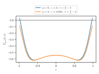
Figure 2: Example form of the function $\tilde{\Gamma}_{p,\epsilon}(t,r)$ at $t=\frac{2}{3}-\delta$ for a small $\delta$ ($\delta=1/p^{2}$ in above), as analyzed in Lemma 16. For any $\epsilon>0$ it is possible to choose a $p$ large enough so that the function lies below $0$ on the relevant domain.

We now consider Laplace’s saddle point method (e.g., see [But07] Chapter 2) for evaluating this integral, which gives (denoting our region of integration $S$):

$$\int_{S}\differential{S}\exp\left(f(t,g,r)n\right)h(t,r)=(1+o(1))\left(\frac{2\pi}{n}\right)^{\frac{3}{2}}\frac{\exp(f(\hat{t},\hat{g},\hat{r})n)}{\sqrt{-\det\nabla^{2}f(\hat{t},\hat{g},\hat{r})}}h(\hat{t},\hat{r}),$$ (136)

where $\hat{t},\hat{g},\hat{r}=\operatorname*{arg\,max}_{t,g,r\in S}f(t,g,r)$. We will show in Lemma 16 that $\hat{t}=\hat{g}=\hat{r}=0$ for an appropriate choice of $\epsilon$, such that:

$$f(\hat{t},\hat{g},\hat{r}) =0,$$ (137)

$$h(\hat{r}) =\sqrt{3}+o(1).$$ (138)

We also calculate:

$$-\det\nabla^{2}f(\hat{t},\hat{g},\hat{r})=81.$$ (139)

Thus,

$$\frac{\mathbb{E}\left[N_{\epsilon}^{2}\right]}{\mathbb{E}\left[N_{\epsilon}\right]^{2}}\leq(1+o(1))\left(\frac{2\pi}{n}\right)^{-\frac{3}{2}}\left(\frac{2\pi}{n}\right)^{\frac{3}{2}}\frac{3\sqrt{3}}{9}\sqrt{3}=1+o(1).$$ (140)

Lemma 16.

For every $\epsilon>0$ there exists large enough $p$ such that the function

$$\Lambda_{p,\epsilon}(t,g,r)=2^{\left(\frac{2}{3}-t\right)n}\binom{\left(t+\frac{1}{3}\right)n}{\frac{\left(t+\frac{1}{3}+r\right)n}{2}}\binom{n}{\frac{n}{3}+tn,\frac{n}{3}+gn,\frac{n}{3}-tn-gn}\exp_{6}\left(-n+\frac{2(1-\epsilon)^{2}}{1+r^{-p}}n\right)$$ (141)

over the domain $t\in\left[-\frac{1}{3},\frac{2}{3}\right],g\in\left[-\frac{1}{3},\frac{1}{3}-t\right],r\in[-\left(t+\frac{1}{3}\right),t+\frac{1}{3}]$ achieves its maximum at $t,g,r=0$ in the limit of large $n$.

Proof.

For any given $t$, note that the maximum over $g$ is when $g=-\frac{t}{2}$, so we can reduce this to an optimization over $t,r$. Note also that the function is even in $r$ for $p$ even, and for $p$ odd monotonically decreases as $r\to^{+}-1$, so we may also consider $r\in\left[0,t+\frac{1}{3}\right]$ without loss of generality.

From Stirling’s approximation we have that

$$\binom{\left(t+\frac{1}{3}\right)n}{\frac{\left(t+\frac{1}{3}+r\right)n}{2}}=\exp_{6}\left(\left(\left(t+\frac{1}{3}\right)H_{6}\left(\frac{1+\frac{r}{t+\frac{1}{3}}}{2}\right)+o(1)\right)n\right),$$ (142)

where $H_{6}(p)=-p\log_{6}(p)-(1-p)\log_{6}(1-p)$ is the binary entropy function in logarithmic base $6$. We also have that:

$$\binom{n}{\frac{n}{3}+tn,\frac{n}{3}-\frac{tn}{2},\frac{n}{3}-\frac{tn}{2}}=\exp_{6}\left(\left(H_{6}\left(\frac{1}{3}+t,\frac{1}{3}-\frac{t}{2},\frac{1}{3}-\frac{t}{2}\right)+o(1)\right)n\right),$$ (143)

where $H_{6}\left(p_{1},p_{2},p_{3}\right)=-\sum\limits_{i=1}^{3}p_{i}\log_{6}\left(p_{i}\right)$ is the entropy function in logarithmic base $6$. Thus, we have that

$$\Lambda_{p,\epsilon}\left(t,r\right)=\exp_{6}\left(\left(H_{6}\left(\frac{1}{3}+t,\frac{1}{3}-\frac{t}{2},\frac{1}{3}-\frac{t}{2}\right)+\left(t+\frac{1}{3}\right)H_{6}\left(\frac{1+\frac{r}{t+\frac{1}{3}}}{2}\right)+\frac{2(1-\epsilon)^{2}}{1+r^{-p}}-1+\left(\frac{2}{3}-t\right)\log_{6}\left(2\right)+o(1)\right)n\right).$$ (144)

We define its leading-order exponent for simplicity:

$$\tilde{\Lambda}_{p,\epsilon}\left(t,r\right)=H_{6}\left(\frac{1}{3}+t,\frac{1}{3}-\frac{t}{2},\frac{1}{3}-\frac{t}{2}\right)+\left(t+\frac{1}{3}\right)H_{6}\left(\frac{1+\frac{r}{t+\frac{1}{3}}}{2}\right)+\frac{2(1-\epsilon)^{2}}{1+r^{-p}}-1+\left(\frac{2}{3}-t\right)\log_{6}\left(2\right).$$ (145)

We will proceed by considering two cases: first when $t\in\left[-\frac{1}{3},\frac{2}{3}-\frac{3}{p^{2}}\right]$, and then when $t\in\left(\frac{2}{3}-\frac{3}{p^{2}},\frac{2}{3}\right]$.

First consider the upper-bound on $\tilde{\Lambda}_{p,\epsilon}$:

$$\tilde{\Upsilon}_{p,\epsilon}(t,r)=H_{6}\left(\frac{1}{3}+t,\frac{1}{3}-\frac{t}{2},\frac{1}{3}-\frac{t}{2}\right)+\frac{1}{3}H_{6}\left(\frac{1+r}{2}\right)+\frac{2(1-\epsilon)^{2}}{1+r^{-p}}-1+\frac{2}{3}\log_{6}\left(2\right).$$ (146)

Note that $\tilde{\Lambda}_{p,\epsilon}\left(0,0\right)=\tilde{\Upsilon}_{p,\epsilon}\left(0,0\right)=0$. We fix $t$. We have the upper-bound:

$$H_{6}\left(\frac{1+r}{2}\right)\leq\log_{6}(2)\sqrt{1-r^{2}}.$$ (147)

The associated upper-bound on $\tilde{\Upsilon}_{p,\epsilon}(t,r)$ at this fixed $t$ thus has a critical point for $r\in\left(0,1\right]$ when:

$$2\left(1-\epsilon\right)^{2}p\sqrt{1-r^{2}}-\frac{1}{3}\log_{6}(2)r^{p+1}\left(1+r^{-p}\right)^{2}=0.$$ (148)

Assuming $\epsilon$ is bounded away from $1$, it is straightforward to check that

$$r=1-\frac{2\log_{6}(2)^{2}}{9p^{2}\left(1-\epsilon\right)^{4}}+O\left(\frac{1}{p^{3}}\right)$$ (149)

solves Equation 148 to leading order. In particular, for sufficiently large $p$, for $t\leq\frac{2}{3}-\frac{3}{p^{2}}$, $\tilde{\Upsilon}_{p,\epsilon}$ has no critical points in $r$ on the interval $\left(0,t+\frac{1}{3}\right]$; thus, $\tilde{\Upsilon}_{p,\epsilon}$ is maximized only at $r=0$ for such $t$, and therefore it is easy to see is maximized only at $r=t=0$. As $\tilde{\Upsilon}$ upper-bounds $\tilde{\Lambda}$ (and equals $\tilde{\Lambda}$ at $r=t=0$), this also implies that $\tilde{\Lambda}$ is maximized only at $r=t=0$ for $t\in\left[-\frac{1}{3},\frac{2}{3}-\frac{3}{p^{2}}\right],r\in\left[-\left(t+\frac{1}{3}\right),t+\frac{1}{3}\right]$.

Now consider when $\frac{2}{3}-\frac{3}{p^{2}}<t\leq\frac{2}{3}$. In this regime we have the alternative upper-bound on $\Lambda_{p,\epsilon}$:

$$\tilde{\Gamma}_{p,\epsilon}\left(t,r\right)=H_{6}\left(\frac{1}{3}+t,\frac{1}{3}-\frac{t}{2},\frac{1}{3}-\frac{t}{2}\right)+H_{6}\left(\frac{1+r}{2}\right)+\frac{2(1-\epsilon)^{2}}{1+r^{-p}}-1+\frac{3}{p^{2}}\log_{6}\left(2\right).$$ (150)

Example plots $\tilde{\Gamma}_{p,\epsilon}$ at fixed $t$ are given in Fig. 2. If we show this is strictly less than $0$ for $t\in\left(\frac{2}{3}-\frac{3}{p^{2}},\frac{2}{3}\right],r\in\left(0,t+\frac{1}{3}\right]$ (for sufficiently large $p$), we will have shown the desired result.

The first entropy term is maximized at $t=\frac{2}{3}-\frac{3}{p^{2}}$, where:

$$H_{6}\left(\frac{1}{3}+t,\frac{1}{3}-\frac{t}{2},\frac{1}{3}-\frac{t}{2}\right) =H_{6}\left(\frac{3}{p^{2}}\right)+\frac{3\log_{6}(2)}{p^{2}}$$ (151)

$$\leq\log_{6}(2)\left(\frac{12}{p^{2}}\left(1-\frac{3}{p^{2}}\right)\right)^{\frac{1}{\ln\left(4\right)}}+\frac{3\log_{6}(2)}{p^{2}}.$$

For sufficiently large $p$, the desired bound is satisfied when:

$$\left(1-\epsilon\right)^{2}<\left(1-\frac{3}{p^{2}}\log_{6}\left(2\right)-\log_{6}(2)\left(\frac{12}{p^{2}}\left(1-\frac{3}{p^{2}}\right)\right)^{\frac{1}{\ln\left(4\right)}}-\frac{3\log_{6}(2)}{p^{2}}-\log_{6}(2)\sqrt{1-r^{2}}\right)\left(1+r^{-p}\right)$$ (152)

for all $0<r\leq 1$. Once again minimizing this bound over $r$, we find that it has a critical point when:

$$r^{2}\left(1+r^{p}\right)+p\left(1-r^{2}-\log_{2}(6)\left(1-\log_{6}(2)\left(\frac{12}{p^{2}}\left(1-\frac{3}{p^{2}}\right)\right)^{\frac{1}{\ln\left(4\right)}}-\frac{3\log_{6}(2)}{p^{2}}\right)\sqrt{1-r^{2}}\right)=0.$$ (153)

It is straightforward to check that

$$r=1-\frac{2\log_{6}\left(2\right)^{2}}{p^{2}}+O\left(\frac{1}{p^{3}}\right)$$ (154)

solves Equation 153 up to terms of the order $O\left(\frac{1}{p^{2}}\right)$. To leading nontrivial order in $p$, then,

$$\left(1-\epsilon\right)^{2}<\frac{1}{2}\left(1-\frac{2\log_{6}(2)}{p}+O\left(p^{-\frac{2}{\ln\left(4\right)}}\right)\right)2=1-\frac{2\log_{6}(2)}{p}+O\left(p^{-\log_{2}\left(\mathrm{e}\right)}\right)$$ (155)

suffices. That is, one can take any $p$ such that

$$\epsilon>\frac{\log_{6}(2)}{p}+O\left(p^{-\log_{2}\left(\mathrm{e}\right)}\right)=\frac{\log_{6}(2)}{p}+o\left(p^{-1.44}\right).$$ (156)

∎

6 Existence of maximum energy limit for product states

Throughout this study, we are considering the limiting maximum energy over product states:

$$\lim_{n\to\infty}\mathbb{E}\frac{1}{\sqrt{n}}\max_{\ket{\phi}\in\mathcal{S}}\bra{\phi}H_{n,p}\ket{\phi}.$$ (157)

To justify the existence of this limit (for even $p$), we extend classical techniques showing super-additivity of the energy in the Sherrington–Kirkpatrick model [Tal10, GT02], a condition which guarantees the existence of the limit by Fekete’s Lemma [Fek23]. For our purposes, we will use a weaker notion of near super-additivity which also guarantees the existence of the limit [DBE51] (see Lemma 19).

Definition 17 (Near super-additive sequence).

A sequence of numbers ${a_{n}}$ is near super-additive if there exists some function $f:\mathbb{R}^{+}\to\mathbb{R}^{+}$ satisfying

$$\int_{1}^{\infty}\frac{f(t)}{t^{2}}\;dt<\infty$$ (158)

such that $a_{n+m}\geq a_{n}+a_{m}-f(n+m)$ for all $n,m>0$.

Our proof will show that the maximum energy of the Hamiltonian $H_{n,p}$ is near super-additive. Formally, we are only able to prove the existence of the limit for even $p$ as our proof relies on convexity of the covariance function for even $p$.

Lemma 18 (Existence of limit).

In the $p$-spin Hamiltonian model defined in Equation 3, for even $p$, the limit

$$\lim_{n\to\infty}\mathbb{E}\frac{1}{\sqrt{n}}\max_{\ket{\phi}\in\mathcal{S}}\bra{\phi}H_{n,p}\ket{\phi}$$ (159)

exists for both the set of all product states $\mathcal{S}=\mathcal{S}_{\rm product}^{n}$ and the set of all product states in the Pauli basis $\mathcal{S}=\mathcal{S}_{\rm Pauli}^{n}$.

To prove the limit exists, we consider the interpolating Hamiltonian $H_{t}$ defined as

$$H_{t}=\sqrt{t}\sqrt{n+m}H_{n+m,p}+\sqrt{1-t}\left(\sqrt{n}H_{n,p}+\sqrt{m}H_{m,p}\right),$$ (160)

where w.l.o.g. we assume that $H_{n,p}$ is supported on the first $n$ qubits and $H_{m,p}$ is supported on qubits $n+1,\dots,n+m$. Here, the Hamiltonians $H_{n,p},H_{m,p},H_{n+m,p}$ all have coefficients drawn independently from each other.

This Hamiltonian interpolates between $H_{0}=\sqrt{n}H_{n,p}+\sqrt{m}H_{m,p}$ and $H_{1}=\sqrt{n+m}H_{n+m,p}$. Given a finite set of states $\mathcal{S}$, we also define the quantities

$$\varphi(t)=\frac{1}{n+m}\beta^{-1}\mathbb{E}\log Z_{\beta}(t),\quad Z_{\beta}(t)=\sum_{\ket{\phi}\in\mathcal{S}}\exp\left(\beta\bra{\phi}H_{t}\ket{\phi}\right)$$ (161)

as the normalized free energy and partition function of the interpolating Hamiltonian respectively. Later, we will set $\mathcal{S}$ equal to either the set of Pauli basis states or some $\epsilon$-cover over the set of product states. The interpolating Hamiltonian also allows one to interpolate between the free energy of the full system and subsystem. Accordingly, we define the free energy terms of the full system as

$$F_{\beta,n+m}\coloneqq\beta^{-1}\mathbb{E}\log Z_{\beta,n+m}=\beta^{-1}\mathbb{E}\left[\log\sum_{\ket{\phi}\in\mathcal{S}}\exp\left(\beta\bra{\phi}\sqrt{n+m}H_{n+m,p}\ket{\phi}\right)\right].$$ (162)

Similar statements hold for the subsystem free energies $F_{\beta,n}$ and $F_{\beta,m}$. Note that $F_{\beta,n+m}=(n+m)\varphi(1)$.

Classical proofs of the existence of the limit for the Sherrington–Kirkpatrick model show that the limit exists by proving the super-additivity of the free energy and applying Fekete’s Lemma [Fek23]. We will use an enhancement of Fekete’s Lemma from de Bruijn and Erdős [DBE51] which guarantees the existence of the limit for near super-additive sequences [DBE51, FR20] (see also Theorem 1.9.2 of [Ste97]).

Lemma 19 (de Bruijn–Erdős extension of Fekete’s Lemma [DBE51]).

For every near super-additive sequence $\{a_{n}\}$ (see Definition 17), the limit $\lim_{n\to\infty}\frac{a_{n}}{n}$ exists and is equal to

$$\lim_{n\to\infty}\frac{a_{n}}{n}=\sup_{n\geq 1}\frac{a_{n}}{n}.$$ (163)

Our goal is to prove near super-additivity of the free energy and extend this to show that the maximum energy is also near super-additive. Both of these will be consequences of the near convexity of the covariance functions for the Hamiltonian $H_{n,p}$.

Lemma 20 (Near super-additivity of free energy (adapted from Theorem 1.1 of [Pan13])).

For a constant $c>0$, the normalized interpolating free energy $\varphi(t)$ satisfies the relation

$$\varphi(1)\geq\varphi(0)-\frac{\beta c}{n+m}.$$ (164)

Proof.

The derivative of $\varphi(t)$ with respect to $t$ satisfies

$$\varphi^{\prime}(t)=(n+m)^{-1}\beta^{-1}\mathbb{E}\left[\left\langle\beta\frac{\partial}{\partial t}\bra{\phi}H_{t}\ket{\phi}\right\rangle_{\ket{\phi}\in\mathcal{S}}\right],$$ (165)

where

$$\left\langle f(\ket{\phi})\right\rangle_{\ket{\phi}\in\mathcal{S}}\coloneqq\sum_{\ket{\phi}\in\mathcal{S}}\frac{\exp\left(\beta\bra{\phi}H_{t}\ket{\phi}\right)}{Z_{\beta}(t)}f(\ket{\phi})$$ (166)

denotes the average of the function $f:\mathcal{S}\to\mathbb{R}$ with respect to the Gibbs measure. We can evaluate the expectation of the Gibbs average via standard formulas derived by Gaussian integration by parts (see Lemma 1.1 in [Pan13]), giving

$$\varphi^{\prime}(t)=(n+m)^{-1}\beta\mathbb{E}\left[\left\langle\mathbb{E}\left[\bra{\phi}H_{t}\ket{\phi}\frac{\partial}{\partial t}\bra{\phi}H_{t}\ket{\phi}\right]-\mathbb{E}\left[\bra{\phi}H_{t}\ket{\phi}\frac{\partial}{\partial t}\bra{\psi}H_{t}\ket{\psi}\right]\right\rangle_{\ket{\phi},\ket{\psi}\in\mathcal{S}}\right].$$ (167)

Evaluating the derivative, we note that

$$\begin{split}\mathbb{E}\left[\bra{\phi}H_{t}\ket{\phi}\frac{\partial}{\partial t}\bra{\psi}H_{t}\ket{\psi}\right]&=\frac{n+m}{2}\mathbb{E}\left[\bra{\phi}H_{n+m,p}\ket{\phi}\bra{\psi}H_{n+m,p}\ket{\psi}\right]\\ &\quad-\frac{n}{2}\mathbb{E}\left[\bra{\phi}H_{n,p}\ket{\phi}\bra{\psi}H_{n,p}\ket{\psi}\right]-\frac{m}{2}\mathbb{E}\left[\bra{\phi}H_{m,p}\ket{\phi}\bra{\psi}H_{m,p}\ket{\psi}\right].\end{split}$$ (168)

Lemma 21 evaluates the variance and covariance terms above. Namely, we have

$$\begin{split}\varphi^{\prime}(t)=-(n+m)^{-1}\frac{\beta}{2}\mathbb{E}\biggl{\langle}&\mathbb{E}\left[(n+m)\bra{\phi}H_{n+m,p}\ket{\phi}\bra{\psi}H_{n+m,p}\ket{\psi}\right]\\ &-\mathbb{E}\left[n\bra{\phi}H_{n,p}\ket{\phi}\bra{\psi}H_{n,p}\ket{\psi}\right]-\mathbb{E}\left[m\bra{\phi}H_{m,p}\ket{\phi}\bra{\psi}H_{m,p}\ket{\psi}\right]\biggr{\rangle}_{\ket{\phi},\ket{\psi}\in\mathcal{S}}.\end{split}$$ (169)

Applying the inequality in Lemma 21 with a constant $c>0$,

$$\begin{split}\varphi^{\prime}(t)\geq-(n+m)^{-1}\frac{\beta}{2}c.\end{split}$$ (170)

Integrating from $t=0$ to $t=1$ completes the proof. ∎

The previous Lemma proves that the free energy is near super-additive. Using standard bounds relating the free energy to the maximum energy, we can extend this near super-additivity to the maximum energy as well to prove Lemma 18.

Proof of Lemma 18.

For a given finite set of product states $\mathcal{S}$, let $\hat{E}_{n+m}$ denote the maximum energy defined as

$$\hat{E}_{n+m}\coloneqq\mathbb{E}\max_{\ket{\phi}\in\mathcal{S}}\bra{\phi}\sqrt{n+m}H_{m+n,p}\ket{\phi}.$$ (171)

Similar definitions hold for the maximum energies of the subsystems $\hat{E}_{n}$ and $\hat{E}_{m}$. We have the following standard bounds for $\hat{E}_{n+m}$ in relation to the free energy which hold for any $\beta>0$:

$$F_{\beta,n+m}\geq\hat{E}_{n+m}\geq F_{\beta,n+m}-\frac{\log|\mathcal{S}|}{\beta}.$$ (172)

The first bound follows from noting $\hat{E}_{n+m}=\beta^{-1}\log\exp(\beta\hat{E}_{n+m})\leq F_{\beta,n+m}$. The second bound follows from noting that $\beta^{-1}\log\exp(\beta\hat{E}_{n+m})\geq\beta^{-1}\log(Z_{\beta}/|\mathcal{S}|).$ Furthermore, from Lemma 20, we have that for some $c>0$,

$$F_{\beta,n+m}-F_{\beta,n}-F_{\beta,m}\geq-\beta c.$$ (173)

Combining the previous two equations,

$$\hat{E}_{n+m}-\hat{E}_{n}-\hat{E}_{m}\geq-\beta c-\frac{\log|\mathcal{S}|}{\beta}.$$ (174)

We now separate the proof into two settings where we prove separately the existence of the limit for the maximum over Pauli basis states and all product states.

Pauli basis states

For Pauli basis states, $\log|\mathcal{S}_{\rm Pauli}^{n}|=n\log(6)$. Therefore, setting $\beta=\beta^{\prime}\sqrt{n+m}$ for some $\beta^{\prime}>0$ results in

$$\hat{E}_{n+m}-\hat{E}_{n}-\hat{E}_{m}\geq-\beta^{\prime}c\sqrt{n+m}-\frac{\log 6}{\beta^{\prime}}\sqrt{n+m}.$$ (175)

Since the function $f(n+m)=\beta^{\prime}c\sqrt{n+m}+\frac{\log 6}{\beta^{\prime}}\sqrt{n+m}=o(n+m)$, it meets the conditions of near super-additivity. Applying Lemma 19 completes the proof.

All product states

Let $S_{\epsilon}$ be an $\epsilon$ cover of the pure states on a single qubit. More precisely for any state $\ket{\phi}\in\mathcal{S}_{\rm all}^{1}$ there exists $\ket{\phi^{\prime}}\in S_{\epsilon}$ such that $\|\ket{\phi}-\ket{\phi^{\prime}}\|_{2}\leq\epsilon$. For product states on $n+m$ qubits, we extend the epsilon cover by taking the product of $n+m$ sets $S_{\epsilon}$:

$$S_{\epsilon}^{n+m}=\{\ket{\phi}=\ket{\phi^{(1)}}\otimes\cdots\otimes\ket{\phi^{(n+m)}}\in\mathcal{S}_{\rm product}^{n+m}:\ket{\phi^{(i)}}\in S_{\epsilon}\;\;\forall i\in[n+m]\}.$$ (176)

The $S_{\epsilon}^{n+m}$ guarantees the existence of a product state $\ket{\phi_{\epsilon}}$ within $1-\epsilon(n+m)$ in overlap squared $|\bra{\phi_{\epsilon}}\ket{\phi}|^{2}$ to any product state $\ket{\phi}$. To see this, we choose a $\epsilon$-close state on each qubit $\ket{\phi_{\epsilon}}=\ket{\phi_{\epsilon}^{(1)}}\otimes\cdots\otimes\ket{\phi_{\epsilon}^{(n+m)}}$ and have

$$1-\epsilon\leq\left(1-\frac{\epsilon}{2}\right)^{2}\leq\real\left(\bra{\phi_{\epsilon}^{(i)}}\ket{\phi^{(i)}}\right)^{2}\leq\real\left(\bra{\phi_{\epsilon}^{(i)}}\ket{\phi^{(i)}}\right)^{2}+\imaginary\left(\bra{\phi_{\epsilon}^{(i)}}\ket{\phi^{(i)}}\right)^{2}=\left\lvert\bra{\phi_{\epsilon}^{(i)}}\ket{\phi^{(i)}}\right\rvert^{2},$$ (177)

which implies

$$\left|\bra{\phi_{\epsilon}}\ket{\phi}\right|^{2}\geq(1-\epsilon)^{n+m}\geq 1-\epsilon(m+n).$$ (178)

Using the fact that $\mathbb{E}\lambda_{max}(\sqrt{m+n}H_{m+n,p})=\Theta(m+n)$,

$$\begin{split}\hat{E}_{n+m}&\coloneqq\mathbb{E}\max_{\ket{\phi}\in\mathcal{S}_{\rm product}^{n+m}}\bra{\phi}\sqrt{n+m}H_{m+n,p}\ket{\phi}\\ &\leq\mathbb{E}\max_{\ket{\phi_{\epsilon}}\in S_{\epsilon}^{n+m}}\bra{\phi_{\epsilon}}\sqrt{n+m}H_{m+n,p}\ket{\phi_{\epsilon}}+\Theta(\epsilon(m+n)^{2}),\end{split}$$ (179)

and similarly for the subsystems. Applying this in Equation 174,

$$\hat{E}_{n+m}-\hat{E}_{n}-\hat{E}_{m}\geq-\beta c-\frac{\log|\mathcal{S_{\epsilon}}|^{n+m}}{\beta}-\Theta(\epsilon(m+n)^{2}).$$ (180)

To achieve an $\epsilon$ cover, it suffices to have $|S_{\epsilon}|=(1-2/\epsilon)^{3}$ points (e.g., see Lemma 5.2 of [Ver10]). Therefore, setting $\epsilon=(n+m)^{-k}$ for any fixed $k$,

$$\log|\mathcal{S_{\epsilon}}|^{m+n}=O((m+n)\log(m+n)).$$ (181)

Choosing $k>1$, we have

$$\hat{E}_{n+m}-\hat{E}_{n}-\hat{E}_{m}\geq-\beta c-O(\beta^{-1}(m+n)\log(m+n))-o(m+n).$$ (182)

Setting $\beta=\beta^{\prime}\sqrt{n+m}$ for some constant $\beta^{\prime}$ achieves the required bounds for near super-additivity. Applying Lemma 19 completes the proof. ∎

Finally, we complete the proof of Lemma 18 by proving the near sub-additivity of the subsystem covariance, which was referred to in our proof of Lemma 20.

Lemma 21 (Near sub-additivity of subsystem covariance).

Given product states $\ket{\phi},\ket{\psi}\in\mathcal{S}_{\rm product}^{n+m}$, there exists a constant $c>0$ such that

$$\begin{split}\mathbb{E}\left[(n+m)\bra{\phi}H_{n+m,p}\ket{\phi}\bra{\psi}H_{n+m,p}\ket{\psi}\right]&\leq\mathbb{E}\left[n\bra{\phi}H_{n,p}\ket{\phi}\bra{\psi}H_{n,p}\ket{\psi}\right]\\ &\quad+\mathbb{E}\left[m\bra{\phi}H_{m,p}\ket{\phi}\bra{\psi}H_{m,p}\ket{\psi}\right]+c\end{split}$$ (183)

for even $p$. Additionally, the variance terms satisfy

$$\begin{split}n+m&=\mathbb{E}\left[(n+m)\bra{\phi}H_{n+m,p}\ket{\phi}\bra{\phi}H_{n+m,p}\ket{\phi}\right]\\ &=\mathbb{E}\left[n\bra{\phi}H_{n,p}\ket{\phi}\bra{\phi}H_{n,p}\ket{\phi}\right]+\mathbb{E}\left[m\bra{\phi}H_{m,p}\ket{\phi}\bra{\phi}H_{m,p}\ket{\phi}\right].\end{split}$$ (184)

Proof.

Let $\ket{\phi},\ket{\psi}\in\mathcal{S}_{\rm product}^{n+m}$ where $\ket{\phi}=\ket{\phi^{(1)}}\otimes\cdots\otimes\ket{\phi^{(n+m)}}$ and $\ket{\psi}=\ket{\psi^{(1)}}\otimes\cdots\otimes\ket{\psi^{(n+m)}}$ denote two arbitrary product states. From Lemma 7, we have:

$$\mathbb{E}\left[\bra{\phi}H_{n+m,p}\ket{\phi}\bra{\psi}H_{n+m,p}\ket{\psi}\right]=\frac{1}{\binom{n+m}{p}}\sum_{\bar{\bm{i}}\in\mathcal{I}_{p}^{n+m}}\prod_{k=1}^{p}\left(2\left|\bra{\phi^{(i_{k})}}\ket{\psi^{(i_{k})}}\right|^{2}-1\right).$$ (185)

Using the above, it is straightforward to note that

$$\mathbb{E}\left[(n+m)\left(\bra{\phi}H_{n+m,p}\ket{\phi}\right)^{2}\right]=n+m.$$ (186)

Similar statements hold for the subsystem Hamiltonians $H_{n,p}$ and $H_{m,p}$. For convenience, from here on in the proof, let $R_{k}=\left(2\left|\bra{\phi^{(k)}}\ket{\psi^{(k)}}\right|^{2}-1\right)$. Then,

$$\begin{split}\mathbb{E}[\bra{\phi}(\sqrt{n}H_{n,p}+\sqrt{m}H_{m,p})\ket{\phi}&\bra{\psi}(\sqrt{n}H_{n,p}+\sqrt{m}H_{m,p})\ket{\psi}]\\ &=n{n\choose p}^{-1}E_{p}(R_{1},\dots,R_{n})+m{m\choose p}^{-1}E_{p}(R_{n+1},\dots R_{n+m}),\end{split}$$ (187)

where $E_{p}$ is the $p$-th degree elementary symmetric polynomial defined as

$$E_{p}(x_{1},\dots,x_{n})=\sum_{1\leq i_{1}<\cdots<i_{p}\leq n}x_{i_{1}}x_{i_{2}}\cdots x_{i_{p}}.$$ (188)

Similarly,

$$\mathbb{E}\left[(n+m)\bra{\phi}H_{n+m,p}\ket{\phi}\bra{\psi}H_{n+m,p}\ket{\psi}\right]=(m+n){m+n\choose p}^{-1}E_{p}(R_{1},\dots,R_{n+m}).$$ (189)

We are left with showing the following inequality holds:

$$(m+n)\frac{E_{p}(R_{1},\dots,R_{n+m})}{{m+n\choose p}}\leq n\frac{E_{p}(R_{1},\dots,R_{n})}{{n\choose p}}+m\frac{E_{p}(R_{n+1},\dots,R_{m+n})}{{m\choose p}}+O(1).$$ (190)

Note

$$\frac{(m+n)^{p}}{{m+n\choose p}}=p!+O(1/(m+n)).$$ (191)

Similar identities hold for ${m\choose p}$ and ${n\choose p}$. Thus it suffices to prove that

$$\frac{E_{p}(R_{1},\dots,R_{n+m})}{(m+n)^{p-1}}\leq\frac{E_{p}(R_{1},\dots,R_{n})}{n^{p-1}}+\frac{E_{p}(R_{n+1},\dots,R_{m+n})}{m^{p-1}}+O(1).$$ (192)

We have

$$p!E_{p}(R_{1},\dots,R_{n+m})=\sum_{i_{1}\neq i_{2}\neq\cdots\neq i_{p}}R_{i_{1}}R_{i_{2}}\cdots R_{i_{p}}.$$ (193)

Note that

$$\sum_{i_{1}\neq i_{2}\neq\cdots\neq i_{p}}R_{i_{1}}R_{i_{2}}\cdots R_{i_{p}}=\sum_{1\leq i_{1},\ldots,i_{p}\leq n}R_{i_{1}}R_{i_{2}}\cdots R_{i_{p}}-\sum_{(i_{1},\ldots,i_{p})\in\mathcal{I}_{\rm repeat}}R_{i_{1}}R_{i_{2}}\cdots R_{i_{p}},$$ (194)

where $\mathcal{I}_{\rm repeat}$ denotes the set of tuples $(i_{1},\ldots,i_{p})$ with at least one element repeated. We have that the first sum is $\left(\sum_{1\leq i\leq m+n}R_{i}\right)^{p}$. At the same time, since each $R_{i}$ is bounded by $1$ in absolute value, the sum $\sum_{(i_{1},\ldots,i_{p})\in\mathcal{I}_{\rm repeat}}$ is of the order $O\left((m+n)^{p-1}\right)$. Thus, to show Equation 192, it suffices to verify that

$${\left(\sum_{1\leq i\leq m+n}R_{i}\right)^{p}\over(m+n)^{p-1}}\leq{\left(\sum_{1\leq i\leq m}R_{i}\right)^{p}\over m^{p-1}}+{\left(\sum_{m+1\leq i\leq m+n}R_{i}\right)^{p}\over n^{p-1}}.$$ (195)

We have:

$$\begin{split}{\left(\sum_{1\leq i\leq m+n}R_{i}\right)^{p}\over(m+n)^{p-1}}&=(m+n){\left(\sum_{1\leq i\leq m+n}R_{i}\over m+n\right)^{p}}\\ &=(m+n)\left({m\over m+n}{\sum_{1\leq i\leq m}R_{i}\over m}+{n\over m+n}{\sum_{m+1\leq i\leq m+n}R_{i}\over n}\right)^{p}\\ &\leq(m+n){m\over m+n}\left({\sum_{1\leq i\leq m}R_{i}\over m}\right)^{p}+(m+n){n\over m+n}\left({\sum_{m+1\leq i\leq m+n}R_{i}\over n}\right)^{p}\\ &={\left(\sum_{1\leq i\leq m}R_{i}\right)^{p}\over m^{p-1}}+{\left(\sum_{m+1\leq i\leq m+n}R_{i}\right)^{p}\over n^{p-1}},\end{split}$$ (196)

and the claim is established. The inequality uses the convexity of the function $x^{p}$ for even $p$.

∎

7 Universality of the ground state values

We primarily study random $p$-spin Hamiltonians whose set of coefficients $\bm{\alpha}$ are drawn i.i.d. from the standard normal distribution. Nevertheless, if one is interested in analyzing the asymptotic values of quantities such as the ground state energy or free energy, these coefficients can be changed to a different set $\bm{\alpha}^{\prime}$ with a different distribution to study equivalent models. Proposition 22 states sufficient conditions for which this equivalence holds. For example, any collection of independent distributions where the coefficients $\alpha^{\prime}[\bar{\bm{i}},\bar{\bm{a}}]$ are drawn independently from a bounded random variable with variance 1 and mean 0 suffices. Perhaps more interestingly, one can also consider sparse random Hamiltonians where the active terms are supported on a random hypergraph (e.g., Erdős–-Rényi) model. Here, for example, the coefficients can be distributed proportionally to

$$\alpha^{\prime}[\bar{\bm{i}},\bar{\bm{a}}]\propto\begin{cases}0&\text{ with probability }1-2p_{n}\\ +1&\text{ with probability }p_{n}\\ -1&\text{ with probability }p_{n}\\ \end{cases}$$ (197)

where $p_{n}\in[0,1]$ is the probability that any given Pauli term appears and we require $p_{n}=\omega(n^{-\left(p-1\right)})$ for equivalence to hold due to the boundedness condition in Proposition 22.

Proposition 22 (Equivalence of Hamiltonian models).

Given the random Hamiltonian $H_{n,p}(\bm{\alpha})$ (Equation 3) with coefficients $\alpha[\bar{\bm{i}},\bar{\bm{a}}]\sim\mathcal{N}(0,1)$, let $H_{n,p}(\bm{\alpha}^{\prime})$ denote a random Hamiltonian where the coefficients $\alpha[\bar{\bm{i}},\bar{\bm{a}}]$ are replaced by random variables $\alpha^{\prime}[\bar{\bm{i}},\bar{\bm{a}}]\sim\mathcal{D}_{\bar{\bm{i}},\bar{\bm{a}}}$ drawn independently from a collection of distributions $\mathcal{D}_{\bar{\bm{i}},\bar{\bm{a}}}$. Over the set of quantum states $\mathcal{S}_{\rm all}^{n}$ on $n$ qubits, the limiting average maximum energies are equal under the two distributions

$$\lim_{n\to\infty}\mathbb{E}_{\alpha[\bar{\bm{i}},\bar{\bm{a}}]\sim\mathcal{N}(0,1)}\left[\frac{1}{\sqrt{n}}\max_{\ket{\phi}\in\mathcal{S}_{\rm all}^{n}}\bra{\phi}H_{n,p}(\bm{\alpha})\ket{\phi}\right]=\lim_{n\to\infty}\mathbb{E}_{\alpha^{\prime}[\bar{\bm{i}},\bar{\bm{a}}]\sim\mathcal{D}_{\bar{\bm{i}},\bar{\bm{a}}}}\left[\frac{1}{\sqrt{n}}\max_{\ket{\phi}\in\mathcal{S}_{\rm all}^{n}}\bra{\phi}H_{n,p}(\bm{\alpha}^{\prime})\ket{\phi}\right]$$ (198)

whenever the distributions $\mathcal{D}_{\bar{\bm{i}},\bar{\bm{a}}}$ meet the three conditions:

$$\begin{split}(\text{first moment}):&\quad\mathbb{E}_{\alpha^{\prime}[\bar{\bm{i}},\bar{\bm{a}}]\sim\mathcal{D}_{\bar{\bm{i}},\bar{\bm{a}}}}[\alpha^{\prime}[\bar{\bm{i}},\bar{\bm{a}}]]=0,\\ (\text{second moment}):&\quad\mathbb{E}_{\alpha^{\prime}[\bar{\bm{i}},\bar{\bm{a}}]\sim\mathcal{D}_{\bar{\bm{i}},\bar{\bm{a}}}}[\alpha^{\prime}[\bar{\bm{i}},\bar{\bm{a}}]^{2}]=1,\\ (\text{boundedness}):&\quad\forall\epsilon>0,\;\lim_{n\to\infty}\frac{1}{{n\choose p}}\sum_{\bar{\bm{i}}\in\mathcal{I}_{n}}\sum_{\bar{\bm{a}}\in\{1,2,3\}^{p}}\mathbb{E}[\alpha^{\prime}[\bar{\bm{i}},\bar{\bm{a}}]^{2};|\alpha^{\prime}[\bar{\bm{i}},\bar{\bm{a}}]|>n^{(p-1)/2}\epsilon]=0.\end{split}$$ (199)

7.1 Proof of equivalence

Throughout this section, let $\bm{\alpha}=\{\alpha_{\bar{\bm{i}},\bar{\bm{a}}}\}_{\bar{\bm{i}}\in\mathcal{I}_{p}^{n},\bar{\bm{a}}\in\{1,2,3\}^{p}}$ denote the set of random variables which constitute the coefficients of the random $p$-spin Hamiltonian. All random variables discussed here take values in an open interval $I\subseteq\mathbb{R}$ that contains zero. Here, we treat $H_{n,p}(\bm{\alpha})$ as a random matrix that is a function of a given set of random variables $\bm{\alpha}$.

To prove the equivalence between distributions, we will make use of two linear algebraic facts that allow us to calculate derivatives and bound the free energy in its matrix form.

Lemma 23 (Derivative of matrix exponential [Wil67]).

Given a Hermitian matrix $H_{\theta}\in\mathbb{C}^{n\times n}$ which depends on a parameter $\theta\in\mathbb{R}$,

$$\partial_{\theta}\exp(H_{\theta})=\int_{0}^{1}\exp(tH_{\theta})(\partial_{\theta}H_{\theta})\exp((1-t)H_{\theta})\;dt.$$ (200)

Lemma 24 (Theorem IV.2.5 of [Bha13]).

Given a matrix $A\in\mathbb{C}^{n\times n}$, let $s(A)\in\mathbb{R}^{n}$ denote the vector of singular values of $A$ in descending order. Then for any two matrices $A,B\in\mathbb{C}^{n\times n}$ and any $r>0$,

$$s(A)^{r}s(B)^{r}\succ_{w}s(AB)^{r},$$ (201)

where $\succ_{w}$ indicates that $s(AB)$ is “weakly majorized” (or dominated) by $s(A)s(B)$, i.e.,

$$\sum_{i=1}^{k}s(A)^{r}_{i}s(B)^{r}_{i}\geq\sum_{i=1}^{k}s(AB)^{r}_{i}\;\;\;\text{ for all }k\in[n].$$ (202)

[Cha05] offers a general approach to proving such equivalences of random models, recapitulated in Theorem 26. Before stating this theorem, we define the quantities $\lambda_{r}$ which intuitively bound the magnitude of influence of any given variable on a function or function class.

Definition 25 (Definition 1.1 in [Cha05]).

For any open interval $I$ containing 0, any positive integer $n$, any function $f:I^{n}\to\mathbb{R}$ which is three times differentiable in each coordinate, and $1\leq r\leq 3$, let

$$\lambda_{r}(f)\coloneqq\sup\left\{|\partial_{i}^{p}f({\bm{x}})|^{r/p}:1\leq i\leq n,1\leq p\leq r,{\bm{x}}\in I^{n}\right\},$$ (203)

where $\partial_{i}^{p}$ denotes $p$-fold differentiation with respect to the $i$-th coordinate. For a collection $\mathcal{F}$ of such functions, define $\lambda_{r}(\mathcal{F})\coloneqq\sup_{f\in\mathcal{F}}\lambda_{r}(f)$.

Theorem 26 (Theorem 1.1 of [Cha05]).

Let ${\bm{x}}=(x_{1},\dots,x_{n})\in I^{n}$ and ${\bm{y}}=(y_{1},\dots,y_{n})\in I^{n}$ be two vectors of independent random variables whose first and second moments agree: $\mathbb{E}[x_{i}]=\mathbb{E}[y_{i}]$ and $\mathbb{E}[x_{i}^{2}]=\mathbb{E}[y_{i}^{2}]$ for all $i$. Let $f:I^{n}\to\mathbb{R}$ be a three times differentiable function. Then for any $K>0$,

$$\begin{split}|\mathbb{E}[f({\bm{x}})]-\mathbb{E}[f({\bm{y}})]|\leq&\lambda_{2}(f)\sum_{i=1}^{n}\left[\mathbb{E}[{\bm{x}}_{i}^{2};|x_{i}|>K]+\mathbb{E}[{\bm{y}}_{i}^{2};|y_{i}|>K]\right]\\ &+\lambda_{3}(f)\sum_{i=1}^{n}\left[\mathbb{E}[|{\bm{x}}_{i}|^{3};|x_{i}|\leq K]+\mathbb{E}[|{\bm{y}}_{i}|^{3};|y_{i}|\leq K]\right],\end{split}$$ (204)

where $\lambda_{r}(f)$ is as in Definition 25.

This theorem will be applied to the set of random variables corresponding to the possible energies of the Hamiltonian $H_{n,p}$ over the set of states $\mathcal{S}_{\rm all}^{n}$. The function class $\mathcal{F}$ in our setting will be the energies of these states. More formally, let $f_{\phi}:\mathbb{R}^{{n\choose p}3^{p}}\to\mathbb{R}$ denote the normalized energy of a state as a function of the coefficients $\bm{\alpha}$, defined as

$$f_{\phi}(\bm{\alpha})=\frac{1}{\sqrt{n}}\bra{\phi}H_{n,p}(\bm{\alpha})\ket{\phi}.$$ (205)

The function class $\mathcal{F}_{\mathcal{S}_{\rm all}^{n}}$ contains all such possible functions given the set of states $\mathcal{S}_{\rm all}^{n}$:

$$\mathcal{F}_{\mathcal{S}_{\rm all}^{n}}\coloneqq\{f_{\phi}:\ket{\phi}\in\mathcal{S}_{\rm all}^{n}\}.$$ (206)

In order to prove Proposition 22, we first prove Theorem 27, using the result of Theorem 26 on the free energy.

Theorem 27 (adapted from Theorem 1.4 of [Cha05]).

Given the set of quantum states $\mathcal{S}_{\rm all}^{n}$ on $n$ qubits, denote $U=\max_{f\in\mathcal{F}_{\mathcal{S}_{\rm all}^{n}}}f(\bm{\alpha})$ and $V=\max_{f\in\mathcal{F}_{\mathcal{S}_{\rm all}^{n}}}f(\bm{\alpha}^{\prime})$ as functions of random variables $\bm{\alpha}$ and $\bm{\alpha}^{\prime}$. Then for any $K\geq 0$ and $\beta\geq 1$,

$$\begin{split}\left|\mathbb{E}U-\mathbb{E}V\right|\leq&2\beta^{-1}\log(2^{n})\\ &+2\beta\frac{1}{n{n\choose p}}\sum_{\bar{\bm{i}}\in\mathcal{I}_{p}^{n},\bar{\bm{a}}\in\{1,2,3,\}^{p}}\left[\mathbb{E}[\alpha[\bar{\bm{i}},\bar{\bm{a}}]^{2};|\alpha[\bar{\bm{i}},\bar{\bm{a}}]|>K]+\mathbb{E}[\alpha^{\prime}[\bar{\bm{i}},\bar{\bm{a}}]^{2};|\alpha^{\prime}[\bar{\bm{i}},\bar{\bm{a}}]|>K]\right]\\ &+7\beta^{2}\left(\frac{1}{n{n\choose p}}\right)^{3/2}\sum_{\bar{\bm{i}}\in\mathcal{I}_{p}^{n},\bar{\bm{a}}\in\{1,2,3,\}^{p}}\left[\mathbb{E}[|\alpha[\bar{\bm{i}},\bar{\bm{a}}]|^{3};|\alpha[\bar{\bm{i}},\bar{\bm{a}}]|\leq K]+\mathbb{E}[|\alpha^{\prime}[\bar{\bm{i}},\bar{\bm{a}}]|^{3};|\alpha^{\prime}[\bar{\bm{i}},\bar{\bm{a}}]|\leq K]\right].\end{split}$$ (207)

Proof of Theorem 27.

The proof of this statement follows from [Cha05] replacing sums with traces. For completeness, we replicate the proof and make the relevant changes below. The one major distinction is that the non-commuting nature of the Hamiltonians requires a re-derivation of the bounds for $\lambda_{r}$ for the free energy function. To keep this proof self-contained, we bound those quantities later in Lemma 28.

For $\beta\geq 1$, we have that

$$\begin{split}\max_{\ket{\phi}\in\mathcal{S}_{\rm all}^{n}}\frac{1}{\sqrt{n}}\bra{\phi}H_{n,p}(\bm{\alpha})\ket{\phi}&=\beta^{-1}\log\left[\exp(\beta\max_{\ket{\phi}\in\mathcal{S}_{\rm all}^{n}}f_{\phi}(\bm{\alpha}))\right]\\ &\leq\beta^{-1}\log\Tr[\exp(\frac{1}{\sqrt{n}}\beta H_{n,p}(\bm{\alpha}))]\\ &\leq\beta^{-1}\log\left[2^{n}\exp(\beta\max_{\ket{\phi}\in\mathcal{S}_{\rm all}^{n}}f_{\phi}(\bm{\alpha}))\right].\end{split}$$ (208)

The quantity in the second line $F_{\beta}(\bm{\alpha})\coloneqq\beta^{-1}\log\Tr[\exp(\frac{1}{\sqrt{n}}\beta H_{n,p}(\bm{\alpha}))]$ is the free energy. Given $F(\bm{\alpha})\coloneqq\sup_{f_{\phi}\in\mathcal{F}_{\mathcal{S}_{\rm all}^{n}}}f_{\phi}(\bm{\alpha})$, we have that

$$\left|F(\bm{\alpha})-F_{\beta}(\bm{\alpha})\right|\leq\beta^{-1}\log(2^{n}).$$ (209)

The above implies that

$$\left|\mathbb{E}U-\mathbb{E}V\right|\leq 2\beta^{-1}\log(2^{n})+\left|F_{\beta}(\bm{\alpha})-F_{\beta}(\bm{\alpha}^{\prime})\right|.$$ (210)

We bound the above by using Theorem 26 on the free energy. Using the bounds in Lemma 28 for $\lambda_{2}$ and $\lambda_{3}$ then yields

$$\begin{split}\left|\mathbb{E}U-\mathbb{E}V\right|\leq&2\beta^{-1}\log(2^{n})\\ &+2\beta\frac{1}{n{n\choose p}}\sum_{\bar{\bm{i}}\in\mathcal{I}_{p}^{n},\bar{\bm{a}}\in\{1,2,3,\}^{p}}\left[\mathbb{E}[\alpha[\bar{\bm{i}},\bar{\bm{a}}]^{2};|\alpha[\bar{\bm{i}},\bar{\bm{a}}]|>K]+\mathbb{E}[\alpha^{\prime}[\bar{\bm{i}},\bar{\bm{a}}]^{2};|\alpha^{\prime}[\bar{\bm{i}},\bar{\bm{a}}]|>K]\right]\\ &+7\beta^{2}\left(\frac{1}{n{n\choose p}}\right)^{3/2}\sum_{\bar{\bm{i}}\in\mathcal{I}_{p}^{n},\bar{\bm{a}}\in\{1,2,3,\}^{p}}\left[\mathbb{E}[|\alpha[\bar{\bm{i}},\bar{\bm{a}}]|^{3};|\alpha[\bar{\bm{i}},\bar{\bm{a}}]|\leq K]+\mathbb{E}[|\alpha^{\prime}[\bar{\bm{i}},\bar{\bm{a}}]|^{3};|\alpha^{\prime}[\bar{\bm{i}},\bar{\bm{a}}]|\leq K]\right],\end{split}$$ (211)

which is the desired result. ∎

Lemma 28.

Given the free energy $F_{\beta}(\bm{\alpha})\coloneqq\log\beta^{-1}\Tr[\exp(\frac{1}{\sqrt{n}}\beta H_{n,p}(\bm{\alpha}))]$ corresponding to the random spin glass Hamiltonian, parameters $\lambda_{r}(F_{\beta})$ as defined in Definition 25 are bounded by

$$\begin{split}\lambda_{1}(F_{\beta})\leq\left(\frac{1}{n{n\choose p}}\right)^{1/2},\quad\quad\lambda_{2}(F_{\beta})\leq 2\beta\left(\frac{1}{n{n\choose p}}\right),\quad\quad\lambda_{3}(F_{\beta})\leq 7\beta^{2}\left(\frac{1}{n{n\choose p}}\right)^{3/2}.\end{split}$$ (212)

Proof.

Throughout this, we let $Z_{\beta}$ denote the partition function defined as

$$Z_{\beta}\coloneqq\Tr[\exp\left(\frac{\beta}{\sqrt{n}}H_{n,p}(\bm{\alpha})\right)].$$ (213)

Using Lemma 23 and calculating the first derivative of the free energy $F_{\beta}(\bm{\alpha})$ with respect to parameter $\alpha[\bar{\bm{i}},\bar{\bm{a}}]$, we have

$$\begin{split}\partial_{\alpha[\bar{\bm{i}},\bar{\bm{a}}]}F_{\beta}(\bm{\alpha})&=\frac{1}{\sqrt{n}{n\choose p}^{1/2}Z_{\beta}}\int_{0}^{1}\Tr[\exp\left(t\frac{\beta}{\sqrt{n}}H_{n,p}\right)P_{\bar{\bm{i}}}^{\bar{\bm{a}}}\exp\left((1-t)\frac{\beta}{\sqrt{n}}H_{n,p}\right)]\;dt\\ &=\frac{1}{\sqrt{n}{n\choose p}^{1/2}Z_{\beta}}\Tr[P_{\bar{\bm{i}}}^{\bar{\bm{a}}}\exp\left(\frac{\beta}{\sqrt{n}}H_{n,p}\right)].\end{split}$$ (214)

The second step above uses the cyclic property of the trace. Applying Lemma 24 to upper bound the singular values in the trace, we have

$$\begin{split}\left|\partial_{\alpha[\bar{\bm{i}},\bar{\bm{a}}]}F_{\beta}(\bm{\alpha})\right|&\leq\frac{1}{\sqrt{n}{n\choose p}^{1/2}Z_{\beta}}\Tr[\exp\left(\frac{\beta}{\sqrt{n}}H_{n,p}\right)]\\ &=\frac{1}{\sqrt{n}{n\choose p}^{1/2}}.\end{split}$$ (215)

Similarly, calculating the second derivative using Lemma 23:

$$\begin{split}\partial_{\alpha[\bar{\bm{i}},\bar{\bm{a}}]}^{2}F_{\beta}(\bm{\alpha})&=\frac{1}{\sqrt{n}{n\choose p}^{1/2}Z_{\beta}}\left(\partial_{\alpha[\bar{\bm{i}},\bar{\bm{a}}]}\Tr[P_{\bar{\bm{i}}}^{\bar{\bm{a}}}\exp\left(\frac{\beta}{\sqrt{n}}H_{n,p}\right)]-\frac{1}{Z_{\beta}}\Tr[P_{\bar{\bm{i}}}^{\bar{\bm{a}}}\exp\left(\frac{\beta}{\sqrt{n}}H_{n,p}\right)]\partial_{\alpha[\bar{\bm{i}},\bar{\bm{a}}]}Z_{\beta}\right)\\ &=\underbrace{\frac{1}{\sqrt{n}{n\choose p}^{1/2}Z_{\beta}}\Tr[P_{\bar{\bm{i}}}^{\bar{\bm{a}}}\partial_{\alpha[\bar{\bm{i}},\bar{\bm{a}}]}\exp\left(\frac{\beta}{\sqrt{n}}H_{n,p}\right)]}_{(I)}-\underbrace{\frac{1}{Z_{\beta}^{2}}\frac{\beta}{n{n\choose p}}\Tr[P_{\bar{\bm{i}}}^{\bar{\bm{a}}}\exp\left(\frac{\beta}{\sqrt{n}}H_{n,p}\right)]^{2}}_{(II)},\end{split}$$ (216)

where $\partial_{\alpha[\bar{\bm{i}},\bar{\bm{a}}]}\exp\left(\frac{\beta}{\sqrt{n}}H_{n,p}\right)=\frac{\beta}{\sqrt{n}{n\choose p}^{1/2}}\int_{0}^{1}\exp\left(\frac{\beta t}{\sqrt{n}}H_{n,p}\right)P_{\bar{\bm{i}}}^{\bar{\bm{a}}}\exp\left(\frac{\beta(1-t)}{\sqrt{n}}H_{n,p}\right)\;dt$ from applying Lemma 23. We use the same majorization argument as in Equation 215 to bound the magnitude of the two terms in the above. For the first term, using Lemma 24 and denoting $s_{k}(A)$ as the $k$-th largest singular value of matrix $A$, we have that:

$$\begin{split}|(I)|&\leq\biggl{|}\frac{\beta}{n{n\choose p}Z_{\beta}}\int_{0}^{1}\Tr[P_{\bar{\bm{i}}}^{\bar{\bm{a}}}\exp\left(\frac{\beta t}{\sqrt{n}}H_{n,p}\right)P_{\bar{\bm{i}}}^{\bar{\bm{a}}}\exp\left(\frac{\beta(1-t)}{\sqrt{n}}H_{n,p}\right)]\;dt\biggr{|}\\ &\leq\left|\frac{\beta}{n{n\choose p}Z_{\beta}}\int_{0}^{1}\left[\sum_{k=1}^{2^{n}}s_{k}\left(\exp\left(\frac{\beta t}{\sqrt{n}}H_{n,p}\right)\right)s_{k}\left(\exp\left(\frac{\beta(1-t)}{\sqrt{n}}H_{n,p}\right)\right)\right]\;dt\right|\\ &=\frac{\beta}{n{n\choose p}}.\end{split}$$ (217)

In the above we used the fact that

$$Z_{\beta}=\sum_{k=1}^{2^{n}}s_{k}\left(\exp\left(\frac{\beta t}{\sqrt{n}}H_{n,p}\right)\right)s_{k}\left(\exp\left(\frac{\beta(1-t)}{\sqrt{n}}H_{n,p}\right)\right)$$ (218)

for any $t$. A similar argument shows that the second term in Equation 216 is also bounded in magnitude by the same quantity. Thus, we have $\left|\partial_{\alpha[\bar{\bm{i}},\bar{\bm{a}}]}^{2}F_{\beta}(\bm{\alpha})\right|\leq 2\frac{\beta}{n{n\choose p}}$. Finally, for the third derivative, we have that:

$$\begin{split}\partial_{\alpha[\bar{\bm{i}},\bar{\bm{a}}]}^{3}F_{\beta}(\bm{\alpha})&=\frac{\beta}{n{n\choose p}Z_{\beta}}\Tr[P_{\bar{\bm{i}}}^{\bar{\bm{a}}}\left(\int_{0}^{1}\partial_{\alpha[\bar{\bm{i}},\bar{\bm{a}}]}\left[\exp\left(\frac{\beta t}{\sqrt{n}}H_{n,p}\right)\right]P_{\bar{\bm{i}}}^{\bar{\bm{a}}}\exp\left(\frac{\beta(1-t)}{\sqrt{n}}H_{n,p}\right)\;dt\right)]\\ &\quad+\frac{\beta}{n{n\choose p}Z_{\beta}}\Tr[P_{\bar{\bm{i}}}^{\bar{\bm{a}}}\left(\int_{0}^{1}\exp\left(\frac{\beta t}{\sqrt{n}}H_{n,p}\right)P_{\bar{\bm{i}}}^{\bar{\bm{a}}}\partial_{\alpha[\bar{\bm{i}},\bar{\bm{a}}]}\left[\exp\left(\frac{\beta(1-t)}{\sqrt{n}}H_{n,p}\right)\right]\;dt\right)]\\ &\quad-\frac{\beta}{n{n\choose p}Z_{\beta}^{2}}\partial_{\alpha[\bar{\bm{i}},\bar{\bm{a}}]}[Z_{\beta}]\Tr[P_{\bar{\bm{i}}}^{\bar{\bm{a}}}\left(\int_{0}^{1}\exp\left(\frac{\beta t}{\sqrt{n}}H_{n,p}\right)P_{\bar{\bm{i}}}^{\bar{\bm{a}}}\exp\left(\frac{\beta(1-t)}{\sqrt{n}}H_{n,p}\right)\;dt\right)]\\ &\quad+\frac{2\beta}{n{n\choose p}Z_{\beta}^{2}}\Tr[P_{\bar{\bm{i}}}^{\bar{\bm{a}}}\exp\left(\frac{\beta}{\sqrt{n}}H_{n,p}\right)]\partial_{\alpha[\bar{\bm{i}},\bar{\bm{a}}]}\Tr[P_{\bar{\bm{i}}}^{\bar{\bm{a}}}\exp\left(\frac{\beta}{\sqrt{n}}H_{n,p}\right)]\\ &\quad+\frac{2\beta}{n{n\choose p}Z_{\beta}^{3}}\Tr[P_{\bar{\bm{i}}}^{\bar{\bm{a}}}\exp\left(\frac{\beta}{\sqrt{n}}H_{n,p}\right)]^{2}\partial_{\alpha[\bar{\bm{i}},\bar{\bm{a}}]}Z_{\beta}.\end{split}$$ (219)

The same majorization argument applied earlier can be applied to each term in the sum above to show that $\left|\partial_{\alpha[\bar{\bm{i}},\bar{\bm{a}}]}^{3}F_{\beta}(\bm{\alpha})\right|\leq\frac{7\beta^{2}}{n^{3/2}{n\choose p}^{3/2}}$. Plugging in the bounds on the derivative magnitudes into $\lambda_{r}(F_{\beta})$ in Theorem 26, we arrive at the final result. ∎

Finally, we are ready to prove Proposition 22.

Proof of Proposition 22.

Applying Theorem 27 with $K=\epsilon n^{(p-1)/2}$ and $\beta=An$, and using the bound $\mathbb{E}[|{\bm{x}}_{i}|^{3};|x_{i}|\leq K]\leq K\mathbb{E}[{\bm{x}}_{i}^{2}]$, we get

$$\begin{split}\left|\mathbb{E}U-\mathbb{E}V\right|&\leq C_{1}A^{-1}\\ &\quad+C_{2}\frac{A}{{n\choose p}}\sum_{\bar{\bm{i}},\bar{\bm{a}}}\left[\mathbb{E}[\alpha[\bar{\bm{i}},\bar{\bm{a}}]^{2};|\alpha[\bar{\bm{i}},\bar{\bm{a}}]|>n^{(p-1)/2}\epsilon]+\mathbb{E}[\alpha^{\prime}[\bar{\bm{i}},\bar{\bm{a}}]^{2};|\alpha^{\prime}[\bar{\bm{i}},\bar{\bm{a}}]|>n^{(p-1)/2}\epsilon]\right]\\ &\quad+C_{3}A^{2}{n\choose p}^{-1/2}n^{p/2}\epsilon\end{split}$$ (220)

for some positive constants $C_{1}$, $C_{2}$, and $C_{3}$ independent of $n$. For the last term above, note that

$$\lim_{n\to\infty}{n\choose p}^{-1/2}n^{p/2}=\sqrt{p!}.$$ (221)

Thus, taking the limit of Equation 220 with $n\to\infty$ and using the boundedness assumption on $\bm{\alpha}^{\prime}$, we have that:

$$\lim_{n\to\infty}\left|\mathbb{E}U-\mathbb{E}V\right|\leq C_{1}A^{-1}+C_{3}\sqrt{p!}A^{2}\epsilon.$$ (222)

Since $A$ and $\epsilon$ are arbitrary, the result can be shown by properly taking limits of $A$ and $\epsilon$. ∎

8 Statistical properties of entangled states

One intuition for why product states are effective at optimizing random spin glass Hamiltonians is because on average, product states have exponentially larger variance in comparison to completely random states. Similar intuition was given in [HM17], which studied product state approximations for the ground states of sparse models. Here, we consider the statistical properties of entangled states to more formally describe this intuition and detail the technical challenges in working with entangled states.

Lemma 29 (Variance of random states).

Let $\mathcal{D}_{\mathcal{S}_{\rm all}^{n}}$ denote the uniform distribution over the set of all possible states $\mathcal{S}_{\rm all}^{n}$ on $n$ qubits. The expected variance of the $p$-spin glass Hamiltonian $H_{n,p}$ over this distribution is

$$\mathbb{E}_{\ket{\phi}\sim\mathcal{D}_{\mathcal{S}_{\rm all}^{n}}}\mathbb{E}\left[\left(\bra{\phi}H_{n,p}\ket{\phi}\right)^{2}\right]=\frac{3^{p}}{2^{n}+1}.$$ (223)

Proof.

For a given state $\ket{\phi}\in\mathcal{S}_{\rm all}^{n}$, we have that its variance is

$$\begin{split}\mathbb{E}\left[\left(\bra{\phi}H_{n,p}\ket{\phi}\right)^{2}\right]&=\frac{1}{\binom{n}{p}}\sum_{\bar{\bm{i}}\in\mathcal{I}_{p}^{n}}\sum_{\bar{\bm{a}}\in\{1,2,3\}^{p}}\bra{\phi}P_{\bar{\bm{i}}}^{\bar{\bm{a}}}\ket{\phi}\bra{\phi}P_{\bar{\bm{i}}}^{\bar{\bm{a}}}\ket{\phi}\\ &=\frac{1}{\binom{n}{p}}\sum_{\bar{\bm{i}}\in\mathcal{I}_{p}^{n}}\bra{\phi}\bra{\phi}\left[\sum_{\bar{\bm{a}}\in\{1,2,3\}^{p}}P_{\bar{\bm{i}}}^{\bar{\bm{a}}}\otimes P_{\bar{\bm{i}}}^{\bar{\bm{a}}}\right]\ket{\phi}\ket{\phi}\\ &=\frac{1}{\binom{n}{p}}\sum_{\bar{\bm{i}}\in\mathcal{I}_{p}^{n}}\sum_{\bar{\bm{a}}\in\{1,2,3\}^{p}}\Tr[\ket{\phi}\ket{\phi}\bra{\phi}\bra{\phi}P_{\bar{\bm{i}}}^{\bar{\bm{a}}}\otimes P_{\bar{\bm{i}}}^{\bar{\bm{a}}}].\end{split}$$ (224)

For a given term above, we can take the average over all possible states by replacing the uniform distribution over states with that of the Haar distribution $\mathcal{U}_{2^{n}}$ over the $2^{n}$ dimensional unitary group of matrices:

$$\mathbb{E}_{\ket{\phi}\sim\mathcal{D}_{\mathcal{S}_{\rm all}^{n}}}\mathbb{E}\left[\left(\bra{\phi}H_{n,p}\ket{\phi}\right)^{2}\right]=\frac{1}{\binom{n}{p}}\sum_{\bar{\bm{i}}\in\mathcal{I}_{p}^{n}}\sum_{\bar{\bm{a}}\in\{1,2,3\}^{p}}\Tr\left[\mathbb{E}_{U\sim\mathcal{U}_{2^{n}}}\left[U\otimes U\ket{0}\ket{0}\bra{0}\bra{0}U^{\dagger}\otimes U^{\dagger}\right]P_{\bar{\bm{i}}}^{\bar{\bm{a}}}\otimes P_{\bar{\bm{i}}}^{\bar{\bm{a}}}\right].$$ (225)

The matrix $\mathbb{E}_{U\sim\mathcal{U}_{2^{n}}}\left[U\otimes U\ket{0}\ket{0}\bra{0}\bra{0}U^{\dagger}\otimes U^{\dagger}\right]$ has a closed form that can be evalauted via the Weingarten calculus [CŚ06]. Namely, for our given form, we can use Equation 7.186 of [Wat18] to evaluate this matrix as

$$\begin{split}\mathbb{E}_{U\sim\mathcal{U}_{2^{n}}}\left[U\otimes U\ket{0}\ket{0}\bra{0}\bra{0}U^{\dagger}\otimes U^{\dagger}\right]&=\frac{1}{2{2^{n}+1\choose 2}}\left(I\otimes I+\sum_{a,b=1}^{2^{n}}E_{a,b}\otimes E_{b,a}\right),\end{split}$$ (226)

where $E_{a,b}$ is the indicator matrix equal to one in entry $a,b$ and zero in every other entry. Noting that Pauli matrices are traceless and

$$\Tr\left[\left(\sum_{a,b=1}^{2^{n}}E_{a,b}\otimes E_{b,a}\right)P_{\bar{\bm{i}}}^{\bar{\bm{a}}}\otimes P_{\bar{\bm{i}}}^{\bar{\bm{a}}}\right]=\Tr[P_{\bar{\bm{i}}}^{\bar{\bm{a}}}P_{\bar{\bm{i}}}^{\bar{\bm{a}}}]=2^{n},$$ (227)

we therefore have for any Pauli $P_{\bar{\bm{i}}}^{\bar{\bm{a}}}$ that

$$\begin{split}\Tr\left[\mathbb{E}_{U\sim\mathcal{U}_{2^{n}}}\left[U\otimes U\ket{0}\ket{0}\bra{0}\bra{0}U^{\dagger}\otimes U^{\dagger}\right]P_{\bar{\bm{i}}}^{\bar{\bm{a}}}\otimes P_{\bar{\bm{i}}}^{\bar{\bm{a}}}\right]&=\frac{1}{2{2^{n}+1\choose 2}}2^{n}=\frac{1}{2^{n}+1}.\end{split}$$ (228)

Plugging in the above into Equation 225, we arrive at the final result:

$$\mathbb{E}_{\ket{\phi}\sim\mathcal{D}_{\mathcal{S}_{\rm all}^{n}}}\mathbb{E}\left[\left(\bra{\phi}H_{n,p}\ket{\phi}\right)^{2}\right]=\frac{3^{p}}{2^{n}+1}.$$ (229)

∎

Lemma 29 shows that the variance of the $p$-spin Hamiltonian decays exponentially fast with the number of qubits on average for random states. In fact, noting that the variance function is $\sqrt{3^{p}}$ Lipschitz (see proof in Lemma 9), the variance is also concentrated around this average with high probability. This can equivalently be stated in terms of Levy’s lemma (see Theorem 7.37 of [Wat18]).

Corollary 30.

By Levy’s lemma, for any $\epsilon>0$, there exists a constant $c(p)$ which depends on $p$ but which is independent of $n$ such that

$$\mathbb{P}_{\ket{\psi}\sim\mathcal{D}_{\mathcal{S}_{\rm all}^{n}}}\left[\left|\mathbb{E}\left[\left(\bra{\psi}H_{n,p}\ket{\psi}\right)^{2}\right]-\mathbb{E}_{\ket{\phi}\sim\mathcal{D}_{\mathcal{S}_{\rm all}^{n}}}\mathbb{E}\left[\left(\bra{\phi}H_{n,p}\ket{\phi}\right)^{2}\right]\right|\geq\epsilon\right]\leq 3\exp\left(-c(p)\epsilon^{2}2^{n}\right).$$ (230)

As an aside, the exponential decay in variance also holds over any distribution of states that forms a unitary 2-design [HM23, GAE07]. Furthermore, this exponential decay in the variance has implications for optimizing random spin glass Hamiltonians, and is related to an untrainability phenomenon in quantum variational optimization where it is shown that relevant quantities of optimization typically decay exponentially for collections of random states [MBS⁺18, CAB⁺21, Ans22, AK22].

More generally, the variance of the Hamiltonian with respect to a state $\ket{\phi}$ can be written as a function of the average local purity of the state as detailed below. In this form, the relationship between the entanglement properties of the state and the variance are more apparent. Notably, unlike product states, entangled states can have widely ranging values for the variance. This fact, in part, makes it challenging to prove the existence of the limit of the ground state energy for all states.

Proposition 31 (Variance as function of local purity).

Given a state $\ket{\phi}\in\mathcal{S}_{\rm all}^{n}$, the variance of the energy of the random Hamiltonian for $\ket{\phi}$ is equal to

$$\mathbb{E}\left[\left(\bra{\phi}H_{n,p}\ket{\phi}\right)^{2}\right]=\sum_{k=0}^{p}(-1)^{p-k}2^{k}{p\choose k}A_{k},$$ (231)

where $A_{k}$ is the average purity over all possible subsystems of $k$ qubits. More formally,

$$A_{k}={n\choose k}^{-1}\sum_{S\in{[n]\choose k}}\Tr(\rho_{S}^{2}),$$ (232)

where $\rho_{S}=\Tr_{[n]\setminus S}(\ket{\phi}\bra{\phi})$ is the reduced density matrix of $\ket{\phi}$ for the qubits in $S$ and ${[n]\choose k}$ denotes the set of ordered $k$-tuples drawn without replacement from $[n]$.

Proof.

For a given state $\ket{\phi}\in\mathcal{S}_{\rm all}^{n}$, we have that its variance is

$$\begin{split}\mathbb{E}\left[\left(\bra{\phi}H_{n,p}\ket{\phi}\right)^{2}\right]&=\frac{1}{\binom{n}{p}}\sum_{\bar{\bm{i}}\in\mathcal{I}_{p}^{n}}\sum_{\bar{\bm{a}}\in\{1,2,3\}^{p}}\bra{\phi}P_{\bar{\bm{i}}}^{\bar{\bm{a}}}\ket{\phi}\bra{\phi}P_{\bar{\bm{i}}}^{\bar{\bm{a}}}\ket{\phi}\\ &=\frac{1}{\binom{n}{p}}\sum_{\bar{\bm{i}}\in\mathcal{I}_{p}^{n}}\bra{\phi}\bra{\phi}\left[\sum_{\bar{\bm{a}}\in\{1,2,3\}^{p}}P_{\bar{\bm{i}}}^{\bar{\bm{a}}}\otimes P_{\bar{\bm{i}}}^{\bar{\bm{a}}}\right]\ket{\phi}\ket{\phi}\\ &=\frac{1}{\binom{n}{p}}\sum_{\bar{\bm{i}}\in\mathcal{I}_{p}^{n}}\bra{\phi}\bra{\phi}\left[\prod_{k=1}^{p}\left[2(\operatorname{SWAP})-I\right]_{i_{k},i_{k}+n}\right]\ket{\phi}\ket{\phi},\end{split}$$ (233)

where in the last line we used Equation 31 and use subscripts $\left[2(\operatorname{SWAP})-I\right]_{i,j}$ to indicate that the $\operatorname{SWAP}$ operator acts on qubits $i$ and $j$. As the state $\ket{\phi}$ is no longer necessarily a product state, we let $\rho_{S}$ denote its reduced state on the qubits in the set $S\subseteq[n]$. Furthermore, for $k\in[n]$, we let $A_{k}$ denote the average purity of the state $\ket{\phi}$ over all reduced states supported on $k$ qubits as formally defined in Equation 232. With this notation, we can calculate the variance as

$$\begin{split}\mathbb{E}\left[\left(\bra{\phi}H_{n,p}\ket{\phi}\right)^{2}\right]&=\frac{1}{\binom{n}{p}}\sum_{k=0}^{p}\sum_{\bar{\bm{i}}\in\mathcal{I}_{p}^{n}}(-1)^{p-k}2^{k}\sum_{\{r_{1},\dots,r_{k}\}\in{[p]\choose k}}\Tr(\rho_{\{i_{r_{1}},\dots,i_{r_{k}}\}}^{2})\\ &=\sum_{k=0}^{p}(-1)^{p-k}2^{k}{p\choose k}A_{k}.\end{split}$$ (234)

In the above, we use the fact that the sum over $\bar{\bm{i}}\in\mathcal{I}_{p}^{n}$ is uniform over all possible $p$-tuples, and thus $k$-tuples in turn drawn uniformly from the draws of the $p$-tuples are thus also uniform over all possible $k$-tuples.

∎

The results here show that product states have large variance, though we should caution that product states do not necessarily achieve the maximum variance for the spin glass Hamiltonians $H_{n,p}$. As a simple example, for $n=2$ and $p=2$, the GHZ state $\frac{1}{\sqrt{2}}\left(\ket{00}+\ket{11}\right)$ has higher variance than any product state. However, if we consider a slightly adjusted model $H_{n,(1,\dots,p)}$ which includes all up-to-$p$-local Paulis and is defined as

$$H_{n,(1,\dots,p)}=\frac{1}{2^{p/2}{n\choose p}^{1/2}}\sum_{\bar{\bm{i}}\in\mathcal{I}_{p}^{n}}\sum_{\bar{\bm{a}}\in\{0,1,2,3\}^{p}}\alpha[\bar{\bm{i}};\bar{\bm{a}}]\;P_{\bar{\bm{i}}}^{\bar{\bm{a}}},$$ (235)

then it is straightforward to show that product states maximize the variance of this model. Note, the subtle difference in the above model where the sum $\sum_{\bar{\bm{a}}\in\{0,1,2,3\}^{p}}$ includes identity as well. We also multiply by a constant factor $2^{-p/2}$ to normalize it as variance one for product states.

Lemma 32.

The variance of the energy of the adjusted Hamiltonian $H_{n,(1,\dots,p)}$ for any product state $\ket{\phi}\in\mathcal{S}_{\rm product}^{n}$ is $\mathbb{E}[(\bra{\phi}H_{n,(1,\dots,p)}\ket{\phi})^{2}]=1$ and is the maximum possible variance over the set of all states, i.e., for any state $\ket{\psi}\in\mathcal{S}_{\rm all}^{n}$,

$$\mathbb{E}\left[(\bra{\psi}H_{n,(1,\dots,p)}\ket{\psi})^{2}\right]\leq\mathbb{E}\left[(\bra{\phi}H_{n,(1,\dots,p)}\ket{\phi})^{2}\right]=1.$$ (236)

Proof.

For a given state $\ket{\phi}\in\mathcal{S}_{\rm all}^{n}$ we have that its variance is

$$\begin{split}\mathbb{E}\left[\left(\bra{\phi}H_{n,(1,\dots,p)}\ket{\phi}\right)^{2}\right]&=\frac{1}{\binom{n}{p}2^{p}}\sum_{\bar{\bm{i}}\in\mathcal{I}_{p}^{n}}\sum_{\bar{\bm{a}}\in\{0,1,2,3\}^{p}}\bra{\phi}P_{\bar{\bm{i}}}^{\bar{\bm{a}}}\ket{\phi}\bra{\phi}P_{\bar{\bm{i}}}^{\bar{\bm{a}}}\ket{\phi}\\ &=\frac{1}{\binom{n}{p}2^{p}}\sum_{\bar{\bm{i}}\in\mathcal{I}_{p}^{n}}\bra{\phi}\bra{\phi}\left[\sum_{\bar{\bm{a}}\in\{0,1,2,3\}^{p}}P_{\bar{\bm{i}}}^{\bar{\bm{a}}}\otimes P_{\bar{\bm{i}}}^{\bar{\bm{a}}}\right]\ket{\phi}\ket{\phi}\\ &=\frac{1}{\binom{n}{p}2^{p}}\sum_{\bar{\bm{i}}\in\mathcal{I}_{p}^{n}}\bra{\phi}\bra{\phi}\left[\prod_{k=1}^{p}\left[2(\operatorname{SWAP})\right]_{i_{k},i_{k}+n}\right]\ket{\phi}\ket{\phi},\end{split}$$ (237)

where in the last line we used Equation 31 and use subscripts $\left[2(\operatorname{SWAP})\right]_{i,j}$ to indicate that the $\operatorname{SWAP}$ operator acts on qubits $i$ and $j$. Let $\rho_{S}=\Tr_{[n]\setminus S}(\ket{\phi}\bra{\phi})$ denote the reduced density matrix of $\ket{\phi}$ for the qubits in $S$. Then,

$$\begin{split}\mathbb{E}\left[\left(\bra{\phi}H_{n,(1,\dots,p)}\ket{\phi}\right)^{2}\right]&=\frac{1}{\binom{n}{p}}\sum_{\bar{\bm{i}}\in\mathcal{I}_{p}^{n}}\Tr(\rho_{\{i_{1},\dots,i_{p}\}}^{2}).\end{split}$$ (238)

The above is the sum of purities $0\leq\Tr(\rho_{\{i_{1},\dots,i_{p}\}}^{2})\leq 1$, where the upper bound is saturated for product states. ∎

Appendix A Multinomial Asymptotics

We here prove a simple lemma on the asymptotics of a trinomial coefficient.

Lemma 33 (Trinomial coefficient asymptotics).

For $n$ large,

$$\binom{n}{\frac{n}{3}+t,\frac{n}{3}+g,\frac{n}{3}-t-g}=\left(1+O\left(\frac{1}{n}\right)\right)\frac{\sqrt{3}}{2\pi n}3^{n+1}\exp\left(-\frac{3}{2n}\left(t^{2}+g^{2}+\left(t+g\right)^{2}\right)+O\left(\frac{t^{3}+g^{3}}{n^{2}}\right)\right).$$ (239)

Proof.

We have that:

$$\ln\binom{n}{\frac{n}{3}+t,\frac{n}{3}+g,\frac{n}{3}-t-g}-\ln\binom{n}{\frac{n}{3},\frac{n}{3},\frac{n}{3}} =\ln\left(\prod\limits_{\tilde{t}=1}^{t}\prod\limits_{\tilde{g}=1}^{g}\prod\limits_{\tilde{k}=1}^{t+g}\frac{\frac{n}{3}-\tilde{k}+1}{\left(\frac{n}{3}+\tilde{t}\right)\left(\frac{n}{3}+\tilde{g}\right)}\right)$$ (240)

$$=\sum\limits_{\tilde{k}=1}^{t+g}\ln\left(\frac{n}{3}-\tilde{k}+1\right)-\sum\limits_{\tilde{t}=1}^{t}\ln\left(\frac{n}{3}+\tilde{t}\right)-\sum\limits_{\tilde{g}=1}^{g}\ln\left(\frac{n}{3}+\tilde{g}\right)$$

$$=\frac{3}{n}\left(t+g\right)-\sum\limits_{\tilde{k}=1}^{t+g}\frac{3\tilde{k}}{n}-\sum\limits_{\tilde{t}=1}^{t}\frac{3\tilde{t}}{n}-\sum\limits_{\tilde{g}=1}^{g}\frac{3\tilde{g}}{n}+O\left(\frac{t^{3}+g^{3}}{n^{2}}\right)$$

$$=\frac{3}{n}\left(t+g\right)-\frac{3}{2n}\left(\left(t+g\right)\left(t+g+1\right)+t\left(t+1\right)+g\left(g+1\right)\right)+O\left(\frac{t^{3}+g^{3}}{n^{2}}\right)$$

$$=-\frac{3}{2n}\left(\left(t+g\right)^{2}+t^{2}+g^{2}\right)+O\left(\frac{t^{3}+g^{3}}{n^{2}}\right).$$

As

$$\binom{n}{\frac{n}{3},\frac{n}{3},\frac{n}{3}}=\left(1+O\left(\frac{1}{n}\right)\right)\frac{\sqrt{3}}{2\pi n}3^{n+1}$$ (241)

by Stirling’s approximation, we achieve the desired result. ∎

References

- [ABN23] Anurag Anshu, Nikolas P Breuckmann, and Chinmay Nirkhe. Nlts hamiltonians from good quantum codes. In Proceedings of the 55th Annual ACM Symposium on Theory of Computing, pages 1090–1096, 2023.
- [AK22] Eric R Anschuetz and Bobak T Kiani. Quantum variational algorithms are swamped with traps. Nature Communications, 13(1):7760, 2022.
- [AKS12] Andris Ambainis, Julia Kempe, and Or Sattath. A quantum lovász local lemma. Journal of the ACM (JACM), 59(5):1–24, 2012.
- [Ans22] Eric Ricardo Anschuetz. Critical points in quantum generative models. In Katja Hofmann, Alexander Rush, Yan Liu, Chelsea Finn, Yejin Choi, and Marc Deisenroth, editors, International Conference on Learning Representations. OpenReview, 2022.
- [APD+06] S Anders, MB Plenio, W Dür, Frank Verstraete, and H-J Briegel. Ground-state approximation for strongly interacting spin systems in arbitrary spatial dimension. Physical review letters, 97(10):107206, 2006.
- [BGKT19] Sergey Bravyi, David Gosset, Robert König, and Kristan Temme. Approximation algorithms for quantum many-body problems. Journal of Mathematical Physics, 60(3):032203, 03 2019.
- [BH13] Fernando G.S.L. Brandao and Aram W. Harrow. Product-state approximations to quantum ground states. In Proceedings of the Forty-Fifth Annual ACM Symposium on Theory of Computing, STOC ’13, page 871–880, New York, NY, USA, 2013. Association for Computing Machinery.
- [Bha13] Rajendra Bhatia. Matrix analysis, volume 169. Springer Science & Business Media, 2013.
- [BM80] AJ Bray and MA Moore. Replica theory of quantum spin glasses. Journal of Physics C: Solid State Physics, 13(24):L655, 1980.
- [BMR09] Sergey Bravyi, Cristopher Moore, and Alexander Russell. Bounds on the quantum satisfiability threshold. arXiv preprint arXiv:0907.1297, 2009.
- [Bra11] Sergey Bravyi. Efficient algorithm for a quantum analogue of 2-sat. Contemporary Mathematics, 536:33–48, 2011.
- [BS20] CL Baldwin and B Swingle. Quenched vs annealed: Glassiness from sk to syk. Physical Review X, 10(3):031026, 2020.
- [But07] Ronald W Butler. Saddlepoint approximations with applications, volume 22. Cambridge University Press, 2007.
- [CAB+21] Marco Cerezo, Andrew Arrasmith, Ryan Babbush, Simon C Benjamin, Suguru Endo, Keisuke Fujii, Jarrod R McClean, Kosuke Mitarai, Xiao Yuan, Lukasz Cincio, et al. Variational quantum algorithms. Nature Reviews Physics, 3(9):625–644, 2021.
- [CFCD+23] Chi-Fang, Chen, Alexander M. Dalzell, Mario Berta, Fernando G. S. L. Brandão, and Joel A. Tropp. Sparse random hamiltonians are quantumly easy. arXiv preprint arXiv:2302.03394, 2023.
- [Cha05] Sourav Chatterjee. A simple invariance theorem. arXiv preprint math/0508213, 2005.
- [CŚ06] Benoît Collins and Piotr Śniady. Integration with respect to the haar measure on unitary, orthogonal and symplectic group. Communications in Mathematical Physics, 264(3):773–795, 2006.
- [DBE51] NG De Bruijn and P Erdös. Some linear and some quadratic recursion formulas. i. Indag. Math.(NS), 54(5):374–382, 1951.
- [DGZ23] Yatin Dandi, David Gamarnik, and Lenka Zdeborová. Maximally-stable local optima in random graphs and spin glasses: Phase transitions and universality. arXiv preprint arXiv:2305.03591, 2023.
- [EA75] Samuel Frederick Edwards and Phil W Anderson. Theory of spin glasses. Journal of Physics F: Metal Physics, 5(5):965, 1975.
- [ECP10] Jens Eisert, Marcus Cramer, and Martin B Plenio. Colloquium: Area laws for the entanglement entropy. Reviews of modern physics, 82(1):277, 2010.
- [ES14] László Erdős and Dominik Schröder. Phase transition in the density of states of quantum spin glasses. Mathematical Physics, Analysis and Geometry, 17(3-4):441–464, 2014.
- [Fek23] Michael Fekete. Über die verteilung der wurzeln bei gewissen algebraischen gleichungen mit ganzzahligen koeffizienten. Mathematische Zeitschrift, 17(1):228–249, 1923.
- [FK94] SK Foong and S Kanno. Proof of page’s conjecture on the average entropy of a subsystem. Physical review letters, 72(8):1148, 1994.
- [FL03] Silvio Franz and Michele Leone. Replica bounds for optimization problems and diluted spin systems. Journal of Statistical Physics, 111:535–564, 2003.
- [FR20] Zoltán Füredi and Imre Z Ruzsa. Nearly subadditive sequences. Acta Mathematica Hungarica, 161(2):401–411, 2020.
- [Fri90] A. Frieze. On the independence number of random graphs. Discrete Mathematics, 81:171–175, 1990.
- [FS16] Wenbo Fu and Subir Sachdev. Numerical study of fermion and boson models with infinite-range random interactions. Phys. Rev. B, 94:035135, Jul 2016.
- [FTW19] Renjie Feng, Gang Tian, and Dongyi Wei. Spectrum of syk model. Peking Mathematical Journal, 2:41–70, 2019.
- [GAE07] David Gross, Koenraad Audenaert, and Jens Eisert. Evenly distributed unitaries: On the structure of unitary designs. Journal of mathematical physics, 48(5), 2007.
- [Gam21] David Gamarnik. The overlap gap property: A topological barrier to optimizing over random structures. Proceedings of the National Academy of Sciences, 118(41):e2108492118, 2021.
- [GHL+15] Sevag Gharibian, Yichen Huang, Zeph Landau, Seung Woo Shin, et al. Quantum hamiltonian complexity. Foundations and Trends® in Theoretical Computer Science, 10(3):159–282, 2015.
- [GJ21] David Gamarnik and Aukosh Jagannath. The overlap gap property and approximate message passing algorithms for -spin models. The Annals of Probability, 49(1), 2021.
- [GJK23] David Gamarnik, Aukosh Jagannath, and Eren C Kızıldağ. Shattering in the Ising pure -spin model. arXiv preprint arXiv:2307.07461, 2023.
- [GJW20] David Gamarnik, Aukosh Jagannath, and Alexander S Wein. Low-degree hardness of random optimization problems. In 2020 IEEE 61st Annual Symposium on Foundations of Computer Science (FOCS), pages 131–140. IEEE, 2020.
- [GK12] Sevag Gharibian and Julia Kempe. Approximation algorithms for qma-complete problems. SIAM Journal on Computing, 41(4):1028–1050, 2012.
- [GMZ22] David Gamarnik, Cristopher Moore, and Lenka Zdeborová. Disordered systems insights on computational hardness. Journal of Statistical Mechanics: Theory and Experiment, 2022(11):114015, 2022.
- [GP19] Sevag Gharibian and Ojas Parekh. Almost optimal classical approximation algorithms for a quantum generalization of max-cut. arXiv preprint arXiv:1909.08846, 2019.
- [GT02] Francesco Guerra and Fabio Lucio Toninelli. The thermodynamic limit in mean field spin glass models. Communications in Mathematical Physics, 230:71–79, 2002.
- [HM17] Aram W. Harrow and Ashley Montanaro. Extremal eigenvalues of local Hamiltonians. Quantum, 1:6, April 2017.
- [HM23] Aram W Harrow and Saeed Mehraban. Approximate unitary t-designs by short random quantum circuits using nearest-neighbor and long-range gates. Communications in Mathematical Physics, pages 1–96, 2023.
- [HNP+23] Yeongwoo Hwang, Joe Neeman, Ojas Parekh, Kevin Thompson, and John Wright. Unique games hardness of quantum max-cut, and a conjectured vector-valued borell’s inequality. In Proceedings of the 2023 Annual ACM-SIAM Symposium on Discrete Algorithms (SODA), pages 1319–1384. SIAM, 2023.
- [HS22] Brice Huang and Mark Sellke. Tight lipschitz hardness for optimizing mean field spin glasses. In 2022 IEEE 63rd Annual Symposium on Foundations of Computer Science (FOCS), pages 312–322. IEEE, 2022.
- [Hua21] Yichen Huang. Universal entanglement of mid-spectrum eigenstates of chaotic local hamiltonians. Nuclear Physics B, 966:115373, 2021.
- [Hua22] Yichen Huang. Entanglement dynamics from random product states: Deviation from maximal entanglement. IEEE Transactions on Information Theory, 68(5):3200–3207, 2022.
- [KLW15] Jon P Keating, Noah Linden, and Huw J Wells. Spectra and eigenstates of spin chain hamiltonians. Communications in Mathematical Physics, 338:81–102, 2015.
- [LG19] Tsung-Cheng Lu and Tarun Grover. Renyi entropy of chaotic eigenstates. Physical Review E, 99(3):032111, 2019.
- [LMSS09] Christopher R Laumann, Roderich Moessner, Antonello Scardicchio, and SL Sondhi. Phase transitions and random quantum satisfiability. arXiv preprint arXiv:0903.1904, 2009.
- [MBS+18] Jarrod R McClean, Sergio Boixo, Vadim N Smelyanskiy, Ryan Babbush, and Hartmut Neven. Barren plateaus in quantum neural network training landscapes. Nature communications, 9(1):4812, 2018.
- [Pag93] Don N Page. Average entropy of a subsystem. Physical review letters, 71(9):1291, 1993.
- [Pan13] Dmitry Panchenko. The Sherrington-Kirkpatrick Model. Springer New York, New York, NY, 2013.
- [Par79] Giorgio Parisi. Infinite number of order parameters for spin-glasses. Physical Review Letters, 43(23):1754, 1979.
- [Par80] Giorgio Parisi. A sequence of approximated solutions to the sk model for spin glasses. Journal of Physics A: Mathematical and General, 13(4):L115, 1980.
- [Ros19] Vladimir Rosenhaus. An introduction to the syk model. Journal of Physics A: Mathematical and Theoretical, 52(32):323001, 2019.
- [Sav62] I Richard Savage. Mills’ ratio for multivariate normal distributions. J. Res. Nat. Bur. Standards Sect. B, 66(3):93–96, 1962.
- [Sen18] Subhabrata Sen. Optimization on sparse random hypergraphs and spin glasses. Random Structures & Algorithms, 53(3):504–536, 2018.
- [SGS+22] Paul M Schindler, Tommaso Guaita, Tao Shi, Eugene Demler, and J Ignacio Cirac. Variational ansatz for the ground state of the quantum sherrington-kirkpatrick model. Physical Review Letters, 129(22):220401, 2022.
- [SK75] David Sherrington and Scott Kirkpatrick. Solvable model of a spin-glass. Physical review letters, 35(26):1792, 1975.
- [Spe14] Joel Spencer. Asymptopia, volume 71. American Mathematical Soc., 2014.
- [Ste97] J Michael Steele. Probability theory and combinatorial optimization. SIAM, 1997.
- [SY93] Subir Sachdev and Jinwu Ye. Gapless spin-fluid ground state in a random quantum heisenberg magnet. Physical review letters, 70(21):3339, 1993.
- [Tal06] Michel Talagrand. The parisi formula. Annals of mathematics, pages 221–263, 2006.
- [Tal10] Michel Talagrand. Mean field models for spin glasses: Volume I: Basic examples, volume 54. Springer Science & Business Media, 2010.
- [Ver10] Roman Vershynin. Introduction to the non-asymptotic analysis of random matrices. arXiv preprint arXiv:1011.3027, 2010.
- [VLRK03] Guifre Vidal, José Ignacio Latorre, Enrique Rico, and Alexei Kitaev. Entanglement in quantum critical phenomena. Physical review letters, 90(22):227902, 2003.
- [VMC08] Frank Verstraete, Valentin Murg, and J Ignacio Cirac. Matrix product states, projected entangled pair states, and variational renormalization group methods for quantum spin systems. Advances in physics, 57(2):143–224, 2008.
- [VR17] Lev Vidmar and Marcos Rigol. Entanglement entropy of eigenstates of quantum chaotic hamiltonians. Physical review letters, 119(22):220603, 2017.
- [Wai19] Martin J Wainwright. High-dimensional statistics: A non-asymptotic viewpoint, volume 48. Cambridge university press, 2019.
- [Wat18] John Watrous. The theory of quantum information. Cambridge university press, 2018.
- [Wil67] Ralph M Wilcox. Exponential operators and parameter differentiation in quantum physics. Journal of Mathematical Physics, 8(4):962–982, 1967.