Stability and causality criteria in linear mode analysis:
stability means causality

Abstract

Causality and stability are fundamental requirements for the differential equations describing predictable relativistic many-body systems. In this work, we investigate the stability and causality criteria in linear mode analysis. We discuss the updated stability criterion in $3+1$ dimensional systems and introduce the improved sufficient criterion for causality. Our findings clearly demonstrate that stability implies causality in linear mode analysis. Furthermore, based on the theorems present in this work, we conclude that if updated stability criterion and improved causality criterion are fulfilled in one inertial frame of reference (IFR), they hold for all IFR.

Introduction —

In modern physics, the space-time evolution of predictable relativistic many-body systems is typically described using differential equations. These differential equations must adhere to the principle of causality as required by the theory of relativity [1]. Causality means that signals or information cannot propagate faster than the speed of light. While the physical interpretation of causality is well understood, the establishment of well-defined criteria for causality in various relativistic systems is still rarely discussed. In the context of quantum field theory, it translates into the requirement that the commutators of local operators vanish outside the light cone [2]. For many macroscopic relativistic many-body systems, it is still challenging to derive the general sufficient and necessary criteria for causality, based on our current understanding, also see Refs. [3, 4, 5] and the references therein, for recent developments for the causality criteria in relativistic hydrodynamics.

Another essential prerequisite is stability, characterized by minor perturbations in a state gradually diminishing over time. Typically, one can find solutions to the differential equations near equilibrium or eigenstates. Stability ensures that perturbations near equilibrium or eigenstates return to their respective states. Noteworthy examples for stability include circular orbits in classical central force problem [6], particular solutions in general relativity [7], equilibrium states in thermodynamics [8], and eigenstates of Hamiltonian in quantum mechanics [9], among others.

Analyzing stability and causality helps determine the physical viability of a theory and provides additional constraints on its parameters. One famous example is the relativistic hydrodynamics. The conventional relativistic hydrodynamics up to the first order in the gradient expansion is found to be acausal and unstable [10]. It has, therefore, been extended to second-order formalisms such as MIS [11], BRSSS [12], and DNMR [13] theories. In addition, a stable and causal generalized first-order formalism, the BDNK theory, has also been established [14, 15]. Comprehensive discussions of the causality and stability conditions for these theories can be found in Refs. [16, 3] and the references therein. Moreover, recent interest has emerged in the stability and causality of effective field theory for hydrodynamics [17].

Physically, causality and stability are intertwined. Causality also implies that all physical observables must reside within the light-cone. Assuming there exists a stable mode in one IFR, in which perturbation decays when $t-t_{0}>0$ with $t_{0}$ being initial time. If the perturbation propagates out of the light-cone, we will observe that $t^{\prime}-t_{0}^{\prime}<0$ in another IFR due to a Lorentz transformation. This means that the perturbation grows with time in the second IFR. Therefore, it concludes that acausality leads to unstable mode [18]. The above argument reveals the connection between acausality and unstable modes, the relationship between the causality and stability is worth to be discussed deep. Although the causality and stability conditions overlap in some theories [19], the criteria for causality and stability appear significantly different and seemingly independent. A natural question arises: how can we establish a connection between the stability and causality criteria?

Due to the complexity involved, analyzing the causality and stability of complete differential equations can be challenging. One common approach is to employ linear mode analysis. Despite the significant progress made in recent works [3, 18] regarding stability-causality relations, it remains unclear how to deduce these remarkable findings directly from the basic stability and causality criteria in linear mode analysis.

Let us start the story from the general overview of linear mode analysis. Following that, we discuss the updated stability criteria and introduce improved causality criteria. Finally, we uncover the connection between stability and causality in linear mode analysis based on our findings.

Linear mode analysis and conventional causality and stability criteria —

Linear mode analysis is a widely used method for investigating the stability and causality of differential equations. Here, we take the relativistic hydrodynamics as an illustrative example to introduce the basic idea for linear mode analysis. The main differential equations for relativistic hydrodynamics are the energy-momentum and currents conservation equations, expanded in the gradient expansion. In the linear mode analysis, one considers the perturbations of independent macroscopic variables within the system, e.g. energy density $\delta e$, number density $\delta\rho$, etc., near the equilibrium. Generally, the hydrodynamic conservation equations for $n$ independent perturbations, $\varphi(t,\vec{x})=(\delta e,\delta\rho,...)^{\mathrm{T}}$, on top of the irrotational equilibrium state can be formulated as linear partial differential equations [10]

$$\partial_{t}\varphi(t,\vec{x})+\mathrm{M}(-i\partial)\varphi(t,\vec{x})=0,$$ (1)

where matrix $\mathrm{M}(-i\partial)$ is a polynomial of the space derivative $\partial_{i}$, $\mathrm{M}(-i\partial)=\sum_{j=0}^{N}\mathrm{M}_{(j)}^{i_{1},i_{2},...,i_{j}}\partial_{i_{1}}\partial_{i_{2}}...\partial_{i_{j}}$ with $N\geq 0$ being a finite integer and $\mathrm{M}_{(j)}^{i_{1},i_{2},...,i_{j}}$ being a constant $n\times n$ matrix. For simplicity, plane-wave type perturbations are often adopted in the linear mode analysis,

$$\varphi=\varphi_{0}e^{-i\omega t+i\vec{k}\cdot\vec{x}},\quad\varphi_{0}=\textrm{const.}.$$ (2)

Subsequently, the nonzero solutions to the differential equations (1) exist if and only if

$$0=\mathcal{P}(\omega,\vec{k})\equiv\det[\omega+i\mathrm{M}(\vec{k})].$$ (3)

The eigenvalues of $-i\mathrm{M}(\vec{k})$ yield the dispersion relations, denoted as $\omega_{i}=\omega_{i}(\vec{k})$, $i=1,2,..,n$. Naturally, The dispersion relations should be constrained by physical requirements,

• Stability: all perturbations $|\varphi(0,\vec{x})|$ cannot grow exponentially with time. It gives the conventional stability criterion,

  $$\mathrm{Im}\ \omega\leq 0,\qquad\textrm{for }\vec{k}\in\mathbb{R}^{3},$$ (4)

• Causality: the influence of $\varphi(0,\vec{x})$ propagates no faster than the speed of light. A widely accepted asymptotic causality criterion is [20]

  $$\lim_{|\vec{k}|\rightarrow+\infty}\left\{\frac{|\mathrm{Re}\ \omega|}{|\vec{k}|}\leq 1,\textrm{ |{\hbox{\omega}}/{\hbox{\vec{k}}}| is bounded}\right\},\;\vec{k}\in\mathbb{R}^{3}.$$ (5)

Here, we define the vector norm $|V|\equiv\left(\sum_{i=1}^{j}V_{i}V_{i}^{*}\right)^{1/2}$ for any complex vector $V=(V_{1},V_{2},...,V_{j})$ and adopt notation $\omega=\omega_{i}(\vec{k})$, $i=1,2,..,n$ for brevity moving forward. The causality and stability criteria mentioned above are intuitive, but they are not flawless.

• A practical challenge arises: the conventional causality and stability criteria (4, 5) depend on IFR. Commonly, the causality and stability conditions are first derived from the criteria (4, 5) in the rest frame. Then, the verification of these criteria in other IFR follows. However, this process of examining conditions across different frames is frequently burdensome.

• A concern arises: the conventional causality criterion (5) proves to be inadequate in guaranteeing causality [21].

• A question arises: does stability imply causality? Furthermore, what constitutes the relationship between the stability and the causality criteria?

The aim of this work is to provide improved causality criteria, simplify the steps for Lorentz transformation, bridge the gap between stability and causality criteria, and reveal the profound stability-causality relations. We propose an improved sufficient criterion for causality. This, combined with the new insights into the covariance of the stability and causality criteria, allows for the immediate derivation of significant stability-causality relations in linear mode analysis.

Updated stability criterion for a $3+1$ dimensional relativistic system —

The updated stability criterion for a $3+1$ dimensional relativistic system is,

$$\mathrm{Im}\ \omega\leq|\mathrm{Im}\ \vec{k}|,\quad\text{for }\vec{k}\in\mathbb{C}^{3}.$$ (6)

The inequality (6) is introduced within a $1+1$ dimensional system by imposing the causality on the retarded two-point function in stable systems, as proposed in Ref. [5] and is subsequently proved as the necessary condition for stability across all IFR [22].

The inequality (6) can be proven by employing a contradiction approach. Assuming that $\mathrm{Im}\ \omega>|\mathrm{Im}\ \vec{k}|$ holds true for a specific $\vec{k}$ in one IFR, denoted as $K$, even while maintaining system stability. We perform a special Lorentz transformation from frame $K$ to another IFR $K^{\prime}$, characterized by a velocity $\vec{v}=(\mathrm{Im}\ \vec{k})/(\mathrm{Im\ }\omega)$ relative to $K$. In frame $K^{\prime}$, as $(\omega^{\prime},\vec{k}^{\prime})^{\mathrm{T}}=\Lambda(\vec{v})\cdot(\omega,\vec{k})^{\mathrm{T}}$ with $\Lambda(\vec{v})$ being the Lorentz transformation matrix, we observe that $\mathrm{Im\ }\vec{k}^{\prime}=0$ and $\mathrm{Im}\ \omega^{\prime}=\gamma^{-1}\mathrm{Im}\ \omega>0$ with $\gamma$ being Lorentz factor. It implies the existence of an unstable mode, which violates the stability requirement (4), within the frame $K^{\prime}$. This indicates that the assumption $\mathrm{Im}\ \omega>|\mathrm{Im}\ \vec{k}|$, made in any IFR, can render the system unstable.

Furthermore, the subsequent theorem significantly streamlines the intricate calculations associated with transformations between distinct IFR in linear mode analysis.

Theorem 1.

The stability criterion (6) holds true across all IFR if it is satisfied in a single IFR.

Proof.

It can also been proven by employing a contradiction approach. Assuming $\mathrm{Im}\ \omega^{\prime}\leq|\mathrm{Im}\ \vec{k}^{\prime}|$ holds in a IFR $K^{\prime}$. Let’s suppose that this inequality is violated in another IFR $K^{\prime\prime}$, i.e., there exists $\vec{k}^{\prime\prime}\in\mathbb{C}^{3}$ within frame $K^{\prime\prime}$ for which $\mathrm{Im}\ \omega^{\prime\prime}>|\mathrm{Im}\ \vec{k}^{\prime\prime}|$. By the Lorentz transformation, $(\omega^{\prime\prime},\vec{k}^{\prime\prime})^{\mathrm{T}}=\Lambda(\vec{v})\cdot(\omega^{\prime},\vec{k}^{\prime})^{\mathrm{T}}$ where $\vec{v}$ represents the velocity of frame $K^{\prime\prime}$ relative to $K^{\prime}$, we find

$$|\mathrm{Im}\ \omega^{\prime}|^{2}-|\mathrm{Im}\ \vec{k}^{\prime}|^{2}=|\mathrm{Im}\ \omega^{\prime\prime}|^{2}-|\mathrm{Im}\ \vec{k}^{\prime\prime}|^{2}>0,$$ (7)

and $\mathrm{Im}\ \omega^{\prime}=\gamma(\mathrm{Im}\ \omega^{\prime\prime}-\vec{v}\cdot\mathrm{Im}\ \vec{k}^{\prime\prime})>0$. Thus, we arrive at $\mathrm{Im}\ \omega^{\prime}>|\mathrm{Im}\ \vec{k}^{\prime}|$, which contradicts the original assumption. It means that frame $K^{\prime\prime}$ does not exist. Therefore, the inequality (6) holds across all IFR. ∎

Theorem 1 can also be intuitively comprehended through a geometric lens. Specifically, the vector $\mathrm{Im}(\omega,\vec{k})$ does not lay inside the future lightcone, as discussed in Ref. [22].

Improved sufficient criterion for causality —

Drawing inspiration from the stability criterion (6), we provide a new sufficient criterion for causality based on the theorem below,

Theorem 2.

Suppose that the initial data $\varphi(0,\vec{x})$ for differential equations (1) is smooth with respect to $\vec{x}$, and the volume of the support of $\varphi(0,\vec{x})$ is both finite and non-vanishing. If two constants $R>0$ and $b\in\mathbb{R}$ exist such that

$$\mathrm{Im}\ \omega\leq|\mathrm{Im}\ \vec{k}|+b,\ \textrm{for }|\vec{k}|>R,$$ (8)

then the influence of the initial data propagates with subluminal speed.

Before proving the aforementioned theorem, we intend to present a simplified equivalent version of criterion (8), denoted as follows: If the condition (8) is fulfilled, then there exists an additional real constant $b^{\prime}\geq b$ such that

$$\mathrm{Im}\ \omega\leq|\mathrm{Im}\ \vec{k}|+b^{\prime},\ \textrm{for}\ \vec{k}\in\mathbb{C}^{3}.$$ (9)

Let us deduce the inequality (9) from inequality (8). We notice that the $\omega=\omega(\vec{k})$ must be finite for any finite $|\vec{k}|$. This is because the dispersion relation from the equation (3), represented by $\mathcal{P}(\omega,\vec{k})=\omega^{n}+\sum_{m=0}^{n-1}a_{m}(\vec{k})\omega^{m}=0$ with $a_{m}(\vec{k})$ being a polynomial of $\vec{k}$, will not yield an infinite $\omega$ for finite $\vec{k}$. Consequently, there exists a sufficiently large positive constant $b^{\prime}$ such that $b^{\prime}\geq b$ and $\mathrm{Im}\ \omega\leq|\mathrm{Im}\ \vec{k}|+b^{\prime}$ for $|\vec{k}|\leq R$. Here we have implicitly assumed that the perturbed equations can be written as the form (1), which have already ruled out some acausal equations, e.g., the Benjamin-Bona-Mahony equation [21]. Now, let us direct our attention towards proving the causality criterion (8) with the help of its simplified equivalent version (9).

Proof.

Suppose that the initial data $\varphi(0,\vec{x})$, possessing finite volume, is enclosed within the closed ball centered at $\vec{x}=0$ and having a radius of $L>0$. By employing the general solution of (1), we can express $\varphi(t,\vec{x})$ with $t>0$ as follows,

$$\varphi(t,\vec{x})=\int_{\mathbb{R}^{3}}\frac{d^{3}k}{(2\pi)^{3}}e^{i\vec{k}\cdot\vec{x}}e^{-\mathrm{M}(\vec{k})t}\tilde{\varphi}(0,\vec{k}),$$ (10)

where $\tilde{\varphi}(t,\vec{k})\equiv\int d^{3}xe^{-i\vec{k}\cdot\vec{x}}\varphi(t,\vec{x})$ represents the Fourier transformation of $\varphi(t,\vec{x})$. In this case, the causality means the perturbation $\varphi(t,\vec{x})$ cannot persist beyond the region $|\vec{x}|>L+ct$ with any finite $t>0$, where $c=1$ being the speed of light [1]. Hence, our task is to demonstrate that $\varphi(t,\vec{x})=0$ within the region $|\vec{x}|>L+t$ with any finite $t>0$, given that the dispersion relations adhere to the inequality (8).

The key lies in employing the following two inequalities,

$$||e^{-\mathrm{M}(\vec{k})t}|| \leq \frac{a_{1}}{\epsilon^{n-1}}(1+|\vec{k}|^{N(n-1)})e^{[\lambda(\vec{k})+\epsilon]t},$$ (11)

$$|\tilde{\varphi}(0,\vec{k})| \leq \frac{a_{2}}{1+|\vec{k}|^{N(n-1)+4}}e^{L|\mathrm{Im}\ \vec{k}|},$$ (12)

where $\lambda(\vec{k})\equiv\max_{i}\{\mathrm{Im}\ \omega_{i}(\vec{k})\}$, $\epsilon\in(0,1)$, and $a_{1},a_{2}$ are independent of $t$, $\epsilon$, and $\vec{k}$. Here, the norm $||\cdot||$ is the spectral norm of matrix [23]. The inequality (12) can be obtained by performing integration by parts $N(n-1)+4$ times in $\tilde{\varphi}(t,\vec{k})=\int d^{3}xe^{-i\vec{k}\cdot\vec{x}}\varphi(t,\vec{x})$ [24]. Proof of inequality (11) utilizes the Cauchy integral formula for matrices [25], with details outlined in Appendix A.3.

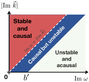
Figure 1: Illustration for stability and causality criteria.

Assisted by these two inequalities, we estimate the integral (10) for $|\vec{x}|>L+t$, employing a method akin to the proof outlined in Theorem 3.1 of Ref. [24]. Upon the fulfillment of the inequality (8) or its simplified equivalent version (9), we have $\lambda(\vec{k})\leq|\mathrm{Im}\ \vec{k}|+b^{\prime}$. Given that the integrand in (10) is an entire analytic function, we change the path $\vec{k}\rightarrow\vec{k}+ir\vec{x}$ and apply Cauchy’s theorem,

$$\left|\varphi(t,\vec{x})\right| = \left|\int_{\mathbb{R}^{3}}d^{3}ke^{i(\vec{k}+ir\vec{x})\cdot\vec{x}}e^{-\mathrm{M}(\vec{k}+ir\vec{x})t}\tilde{\varphi}(0,\vec{k}+ir\vec{x})\right|$$ (13)

$$\propto e^{-r|\vec{x}|(|\vec{x}|-t-L)+(b^{\prime}+\epsilon)t}\rightarrow 0,\text{ as }r\rightarrow+\infty,$$

where we have used (11), (12) and the inequality $|e^{-\mathrm{M}(\vec{k})t}\tilde{\varphi}(0,\vec{k})|\leq||e^{-\mathrm{M}(\vec{k})t}||\cdot|\tilde{\varphi}(0,\vec{k})|$ [23]. Hence, for any given finite $t>0$, we deduce $\varphi(t,\vec{x})=0$ for $|\vec{x}|>L+t$ in accordance with (13), thereby affirming that the perturbation signal propagates at a speed no greater than that of light. ∎

Analogous to the stability criterion, the subsequent theorem facilitates the extension of the causality criterion (8) or (9) from one IFR to all IFR.

Theorem 3.

The causality criterion (8) or (9) holds true across all IFR if it is fulfilled in a single IFR.

Proof.

We prove it by employing a contradiction approach again. Let us focus on the inequality (9). Suppose, by contradiction, that (9) holds in a IFR $K$, but is violated in another IFR $K^{\prime}$, where $K^{\prime}$ moves with a velocity $\vec{v}$ relative to $K$. Thus for any positive real constant $b^{\prime}>0$, there exists a $\vec{k}^{\prime}\in\mathbb{C}^{3}$ such that $\mathrm{Im}\ \omega^{\prime}>|\mathrm{Im}\ \vec{k}^{\prime}|+b^{\prime}$ in frame $K^{\prime}$. Taking Lorentz transformation, we obtain $\mathrm{Im}\ \omega>|\mathrm{Im}\ \vec{k}|+\gamma b^{\prime}(1-|\vec{v}|)$, which contradicts (9) within frame $K$. Therefore, the frame $K^{\prime}$ does not exist. This completes the proof. ∎

In practice, one can verify causality condition by taking $R\rightarrow\infty$ in inequality (8). In large $|\vec{k}|$ limit, the typical dispersion relations exhibit behavior such as $\omega\propto\vec{v}_{0}\cdot\vec{k}+\mathcal{O}(|\vec{k}|^{0}),$ or $\omega\propto c_{0}(\vec{k}\cdot\vec{k})^{1/2}+\mathcal{O}(|\vec{k}|^{0})$, where $c_{0}$ and $\vec{v}_{0}$ are real constants satisfying $|c_{0}|,|\vec{v}_{0}|\in[0,1]$. In this scenario, the sufficient criterion (8) holds, ensuring that the system maintains causality.

The new improved sufficient causality criterion (8) or (9) is more stringent and preferable compared to the conventional insufficient inequality (5). We show that the conventional criterion (5) is automatically fulfilled when the dispersion relations obey the inequality (8) in Appendix A.5. However, the inequality (8) cannot be derived from (5). For example, consider the dispersion relation $\omega=k(1+i)/2$, which indeed satisfies the inequality (5), but does not obey the condition (8). This specific case has been demonstrated to be acausal according to Theorem 2.7 in Ref. [24].

The updated stable criterion (6) and improved casual criterion (8) or (9) offer a straightforward way to reveal the profound relations between stability and causality in linear mode analysis. Consequently, we derive two corresponding conclusions.

Stability in all IFR means causality —

To illustrate the relationship between the stability and causality, we depict the regions that satisfy the stability criterion (6) and causality criterion (9) in Fig. 1. Evidently, the causality criterion (9) is inherently satisfied when the stability criterion (6) holds true in all IFR. However, the reverse does not necessarily hold, e.g. as presented by the blue region in Fig. 1. An example is the tachyon field equation [26], whose dispersion relations fall inside the blue region (also see Appendix A.4). Therefore, stability across all IFR implies causality, while causality does not necessarily entail stability. To prevent any misinterpretation, it is crucial to highlight that if the system has stability solely in specific IFR while being unstable in others, the presence of stability alone does not guarantee causality. The same conclusion has also been substantiated in Refs. [3, 18] through different approaches and also see a preliminary discussion in Ref. [19] written by some of us.

This finding is compatible with another significant observation in Ref. [4] referred to as “thermodynamic stability implies causality”. The conditions for thermodynamic stability delineated as (i)-(iii) in Ref. [4] maintain Lorentz invariance. Clearly, if the thermodynamic stability holds true in a particular IFR, it holds in any IFR.

Stability and causality in one IFR implies stability and causality across all IFR —

The subsequent theorem concerning stability-causality assessment across various frames assists in mitigating the challenge in linear mode analysis, where one is required to examine stability and causality criteria in multiple frames. Similar conclusions have also been reported in Refs. [3, 18], relying on the premise of strong hyperbolicity or causality in all IFR.

Theorem 4.

If the system described by differential equation (1) exhibits stability and causality in one IFR, then it is stable and causal in all IFR.

Proof.

If differential equation (1) is stable and causal in a particular IFR, then it follows that $\mathrm{Im}\ \omega\leq|\mathrm{Im}\ \vec{k}|$ within this frame (see Theorem 2 in Ref. [22] for $1+1$ dimensional case and the Appendix A.6 for $3+1$ dimensional case). Consequently, combining Theorem 1-3 presented in this work completes the proof. ∎

Theorem 4 provides a practical way for evaluating stability and causality across all IFR. Initially, one selects a suitable IFR, e.g. the rest frame in hydrodynamics. One can derive the stability condition by analyzing conventional stability criterion (4) with the Routh-Hurwitz criterion [15], which is often more straightforward than directly assessing stability criterion (6). Subsequently, the causality condition can be verified using the causality criterion (8) as $|\vec{k}|\rightarrow\infty$. To illustrate this point, we provide an example concerning the stability and causality of MIS theory with bulk viscous pressure only, presented in Appendix A.7. Interestingly, the calculations become straightforward in isotropic systems by applying the theorem discussed in the coming paragraph.

Application: Asymptotic criterion for an isotropic system —

Given that numerous discussions revolve around causality and stability within isotropic systems, such as the case of conventional relativistic hydrodynamics in the rest frame, it is fitting for us to examine the stability and causality conditions tailored for isotropic systems, serving as a practical application. In an isotropic system, a simple asymptotic criterion, as presented in the following theorem, becomes a necessary condition for stability and a sufficient condition for causality across all IFR.

Theorem 5.

Considering $\vec{k}=k\hat{\mathrm{n}}$ where $k\in\mathbb{C}$, $\hat{\mathrm{n}}\in\mathbb{C}^{3}$ and $\hat{\mathrm{n}}\cdot\hat{\mathrm{n}}=1$. If the nonzero dispersion relations obtained from the equation (3) are $\hat{\mathrm{n}}$-independent and satisfy inequality (6), then there exists only three asymptotic behaviors at $k\rightarrow\infty$:

$$\omega = c_{1}k+d_{1}+\mathcal{O}(|k|^{a}),$$ (14)

$$\omega = c_{2}k^{-2m-1}+d_{2}k^{-2m-2}+\mathcal{O}(|k|^{a-2m-2}),$$ (15)

$$\omega = c_{3}k^{-2m}+\mathcal{O}(|k|^{a-2m}),$$ (16)

where $a<0$, $m=0,1,2,...$, and $c_{i},d_{i}$ are constants obeying $c_{1}\in[-1,1]$, $\mathrm{Im}\ c_{2}=0$, $\mathrm{Im}\ c_{3}\leq 0$, $\mathrm{Im}\ d_{1,2}\leq 0$.

The proof of above theorem is presented in Appendix A.8 with the help of asymptotic analysis in Ref. [27]. We emphasize that the three dispersion relations (14, 15, 16) mentioned above are necessary conditions for stability. If the asymptotic behaviors of an isotropic system do not adhere to these conditions, it might be causal but must be unstable. Interestingly, the three dispersion relations (14, 15, 16) satisfy the conventional causality criterion (5). This observation helps explain why the conventional causality criterion (5) has been considered a necessary condition for a covariantly stable and causal isotropic system for a long time.

Summary —

In this work we have investigated the updated stability criterion and improved causality criterion for the $3+1$ dimensional relativistic system across all IFR. Notably, our findings indicate that the previously widely used causality criterion (5) needs to be substituted with the improved asymptotic criterion (8) or (9). Based on Theorem 1-3, we reveal the underlying connection between stability and causality in linear mode analysis. Stability in all IFR implies causality, while causality alone does not necessarily require stability. Furthermore, if a system is stable and causal in one IFR, stability and causality holds in all IFR. The findings alleviate the challenge of linear mode analysis, which involves verifying the stability and causality conditions across various frames. As an application, we also study the linear stability and causality of the $3+1$ dimensional isotropic systems and derive the new criterion (14-16) that are necessary for stability and sufficient for causality in all IFR. Finally, it is important to emphasize that our theorems are model-independent and can be applied to other relativistic systems beyond relativistic hydrodynamics.

Appendix A Supplemental Material

A.1 General form of perturbation equations

Generally, the hydrodynamic equations for $n$ independent perturbations, $\varphi(t,\vec{x})=(\delta e,\delta\rho,...)^{\mathrm{T}}$on top of the equilibrium state can be written as the linear partial differential equations

$$\mathrm{A}\partial_{t}\varphi(t,\vec{x})+\mathrm{B}(\partial)\varphi(t,\vec{x})=0.$$ (1)

where $\mathrm{A}$ is a constant $n\times n$ matrix, and matrix $\mathrm{B}(\partial)$ is a polynomial of the space derivative $\partial_{i}$,

$$\mathrm{B}(\partial) = \mathrm{B}_{(0)}+\mathrm{B}_{(1)}^{i_{1}}\partial_{i_{1}}+\mathrm{B}_{(2)}^{i_{1}i_{2}}\partial_{i_{1}}\partial_{i_{2}}$$ (2)

$$+...+\mathrm{B}_{(N)}^{i_{1}i_{2}...i_{N}}\partial_{i_{1}}\partial_{i_{2}}...\partial_{i_{N}},$$

with $N\geq 0$ being a finite integer and $\mathrm{B}_{(j)}^{i_{1}i_{2}...i_{j}}$ being a constant $n\times n$ matrix. The equations including higher order time derivative, such as $\partial_{t}^{2}\varphi$, can be converted into (1) by introducing new variables. Furthermore, for a physical system, the matrix $\mathrm{A}$ must be invertible. Otherwise, the solutions of (1) are not unique or do not exist for given smooth initial conditions $\varphi(0,\vec{x})$. Therefore, we can always write (1) as (1).

A.2 Discussion on inequality (6) from two point Green functions

We now follow Ref. [5] to demenstarte that (6) holds for any complex vector $\vec{k}$. Consider a retarded two point Green function $G^{R}(x,y)$ for certain operators. We take $G^{R}(0,y)$ as a tempered distribution [5]. The causality requires $G^{R}(0,y)$ is only nonzero in the past closed light cone containing the boundary, i.e. $y^{0}\leq-|\vec{y}|<0$. The Fourier transform of $G^{R}(0,y)$ is given by,

$$\tilde{G}^{R}(\omega,\vec{k}) \equiv \int_{y^{0}\leq-|\vec{y}|<0}d^{4}yG^{R}(0,y)\times\exp[(\mathrm{Im}\ \omega)y^{0}$$ (3)

$$-(\mathrm{Im}\ \vec{k})\cdot\vec{y}-i(\mathrm{Re}\ \omega)y^{0}+i(\mathrm{Re}\ \vec{k})\cdot\vec{y}].$$

Let us search for the analytic region for $\tilde{G}^{R}(\omega,\vec{k})$. It means that the exponent in the right handed side of (3) must be suppressed. We find that

$$(\mathrm{Im}\ \omega)y^{0}-(\mathrm{Im}\ \vec{k})\cdot\vec{y} \leq (-\mathrm{Im}\ \omega+|\mathrm{Im}\ \vec{k}|)\cdot|\vec{y}|,\ \textrm{if }\mathrm{Im}\ \omega\geq 0.$$ (4)

Once $\mathrm{Im}\ \omega>|\mathrm{Im}\ \vec{k}|$, it is obvious that exponent is suppressed and $\tilde{G}^{R}(\omega,\vec{k})$ is analytic. The dispersion relation $\omega=\omega(\vec{k})$ as the non-analytic pole of $\tilde{G}^{R}(\omega,\vec{k})$ must be out of region $\mathrm{Im}\ \omega>|\mathrm{Im}\ \vec{k}|$, i.e. it should satisfy inequality (6).

From the above discussion, we start from the requirement of causality and get the stability condition. It implies that the stability and causality are related.

A.3 Proof of the key inequality (11) for causality criterion

We prove inequality (11) here. For an $n\times n$ matrix, we introduce the spectral norm of matrix $||\mathrm{M}||=\sup_{|V^{\prime}|=1}|\mathrm{M}V^{\prime}|$ where $V^{\prime}$ is an arbitrary vector with $|V^{\prime}|=1$ [23].

If $n=1$, we get $\mathrm{M}(\vec{k})=i\omega$ and

$$|e^{-\mathrm{M}(\vec{k})t}|=e^{(\mathrm{Im}\ \omega)t},\quad\textrm{for }n=1.$$ (5)

Next, we consider the case $n>1$. For a fixed complex $\vec{k}$, we have the identity (see chapter 7.3 of Ref. [25])

$$e^{-\mathrm{M}(\vec{k})t}=\frac{1}{2\pi i}\int_{\mathcal{C}}dze^{-zt}[z-\mathrm{M}(\vec{k})]^{-1},$$ (6)

where the path $\mathcal{C}$ is defined as follows. Draw circles of radius $\epsilon\in(0,1)$ centered at $i\omega_{1},i\omega_{2},...,i\omega_{n}$, which are the eigenvalues of the $n\times n$ matrix $\mathrm{M}(\vec{k})$. Then $\mathcal{C}$ is defined as the boundary of the union set of these circles, traversed anticlockwise. We find

$$|e^{-zt}| \leq \exp\left\{\left[\max_{1\leq i\leq n}(\mathrm{Im}\ \omega_{i})+\epsilon\right]t\right\},$$ (7)

$$|\det[z-\mathrm{M}(\vec{k})]| = \prod_{j=1}^{n}|z-i\omega_{j}|\geq\epsilon^{n},\quad\textrm{for }z\in\mathcal{C}.$$ (8)

The spectral norm of the inverse matrix can be evaluated through

$$||[z-\mathrm{M}(\vec{k})]^{-1}|| = \frac{||\mathrm{ad}[z-\mathrm{M}(\vec{k})]||}{|\det[z-\mathrm{M}(\vec{k})]|}$$ (9)

$$\leq \epsilon^{-n}||\mathrm{ad}[z-\mathrm{M}(\vec{k})]||,\quad\textrm{for }z\in\mathcal{C},$$

where $\mathrm{ad}[z-\mathrm{M}(\vec{k})]$ stands for the adjugate matrix of $z-\mathrm{M}(\vec{k})$. Note that the spectral norm is not greater than Frobenius norm [23], i.e.,

$$||\mathrm{ad}[z-\mathrm{M}(\vec{k})]||\leq\left(\sum_{i,j=1}^{n}|\{\mathrm{ad}[z-\mathrm{M}(\vec{k})]\}_{ij}|^{2}\right)^{1/2}.$$ (10)

In the following we estimate the matrix element $|\{\mathrm{ad}[z-\mathrm{M}(\vec{k})]\}_{ij}|$, which equals the absolute value of the determinant of the $(n-1)\times(n-1)$ matrix obtained by deleting the $j$-th row and $i$-th column from $z-\mathrm{M}(\vec{k})$.

To proceed further, we now show that $z\in\mathcal{C}$ is bounded by

$$|z|\leq\mathrm{const}\cdot(1+|\vec{k}|^{N}).$$ (11)

Since the elements in $\mathrm{M}(\vec{k})$ fulfill

$$|\mathrm{M}_{ij}(\vec{k})|\leq\mathrm{const}\cdot(1+|\vec{k}|^{N}),$$ (12)

each eigenvalue $i\omega_{j}$ of $\mathrm{M}(\vec{k})$ is bounded by $|\omega_{j}|\leq\mathrm{const}\cdot(1+|\vec{k}|^{N})$. Recalling that $|z|\leq|\omega_{j}|+1$, we then obtain inequality (11).

The inequalities, (11) and (12), give us

$$|\{\mathrm{ad}[z-\mathrm{M}(\vec{k})]\}_{ij}|\leq\mathrm{const}\cdot(1+|\vec{k}|^{N(n-1)}),\quad\textrm{for }z\in\mathcal{C}.$$ (13)

Hence,

$$||\mathrm{ad}[z-\mathrm{M}(\vec{k})]|| \leq \left(\sum_{i,j=1}^{n}|\{\mathrm{ad}[z-\mathrm{M}(\vec{k})]\}_{ij}|^{2}\right)^{1/2}$$ (14)

$$\leq \mathrm{const}\cdot(1+|\vec{k}|^{N(n-1)}),\quad\textrm{for }z\in\mathcal{C}.$$

According to (7,9,14), we find

$$||[z-\mathrm{M}(\vec{k})]^{-1}|| \leq \epsilon^{-n}||\mathrm{ad}[z-\mathrm{M}(\vec{k})]||$$ (15)

$$\leq \mathrm{const}\cdot\epsilon^{-n}(1+|\vec{k}|^{N(n-1)}),\quad\textrm{for }z\in\mathcal{C}.$$

and, then, obtain

$$||e^{-\mathrm{M}(\vec{k})t}|| = \frac{1}{2\pi}||\int_{\mathcal{C}}dze^{-zt}[z-\mathrm{M}(\vec{k})]^{-1}||$$ (16)

$$\leq \mathrm{const}\cdot\frac{2\pi\epsilon n}{2\pi}\epsilon^{-n}(1+|\vec{k}|^{N(n-1)})\exp\left\{\left[\max_{1\leq i\leq n}(\mathrm{Im}\ \omega_{i})+\epsilon\right]t\right\}$$

$$\leq \mathrm{const}\cdot\epsilon^{1-n}(1+|\vec{k}|^{N(n-1)})\exp\left\{\left[\max_{1\leq i\leq n}(\mathrm{Im}\ \omega_{i})+\epsilon\right]t\right\},\quad\textrm{for }n>1.$$

Combining (5) and (16), we derive the inequality (11). We emphasize that the $\epsilon\in(0,1)$ is arbitrary, and the “const” in (16) is independent of $t$, $\epsilon$, $\omega$, and $\vec{k}$.

A.4 Tachyon field equation is causal but unstable

Tachyon field equation is similar to the Klein-Gordon field equation but with an imaginary mass $im_{0}$ [26], i.e.,

$$(\partial_{t}^{2}-\nabla^{2}-m_{0}^{2})\varphi(x)=0.$$ (17)

This equation can be converted into the form (1), so we can use the results shown in this work to study the stability and causality of Tachyon field.

The dispersion relations of (17) read

$$\omega=\pm(\vec{k}^{2}-m_{0}^{2})^{1/2}.$$ (18)

Obviously, the Tachyon field equation is unstable since one mode has positive imaginary part as $|\vec{k}|\rightarrow 0$.

We then discuss the causality. From (18) we can get

$$(\mathrm{Re}\ \omega)^{2}-(\mathrm{Im}\ \omega)^{2} = (\mathrm{Re}\ \vec{k})^{2}-(\mathrm{Im}\ \vec{k})^{2}-m_{0}^{2},$$ (19)

$$(\mathrm{Re}\ \omega)(\mathrm{Im}\ \omega) = (\mathrm{Re}\ \vec{k})\cdot(\mathrm{Im}\ \vec{k}),$$ (20)

which leads to

$$(\mathrm{Im}\ \omega)^{2} \leq (\mathrm{Im}\ \vec{k})^{2}-\frac{1}{2}(|\vec{k}|^{2}-m_{0}^{2})+\frac{1}{2}\sqrt{(|\vec{k}|^{2}+m_{0}^{2})^{2}-4m_{0}^{2}(\mathrm{Re}\ \vec{k})^{2}}$$ (21)

$$\leq (\mathrm{Im}\ \vec{k})^{2}+m_{0}^{2}.$$

Thus $\mathrm{Im}\ \omega\leq|\mathrm{Im}\ \vec{k}|+m_{0}$ satisfies the improved causality criterion (8) and its equivalent version (9), indicating that the Tachyon field equation (17) is causal indeed.

In fact, there is a simpler way to show that the Tachyon field equation is causal. Since (17) is isotropic, the dispersion relations are independent of the direction of $\vec{k}$. It is enough to study the $1+1$ dimensional propagation. Letting $\vec{k}=(k,0,0)$ in (18), the asymptotic behavior at $k\rightarrow\infty$ is given by

$$\omega=\pm k+\mathcal{O}(|k|^{-1}),$$ (22)

which satisfies the asymptotic behaviors in Theorem 5. For any $\epsilon>0$, we can find a large number $R$ such that $\mathrm{Im}[\mathcal{O}(|k|^{-1})]<\epsilon$ for $|k|>R$. Therefore $\mathrm{Im}\ \omega<|\mathrm{Im}\ k|+\epsilon$ for $|k|>R$, and then the Tachyon field equation is causal according to the causality criterion (8).

A.5 Relation between the improved causality criterion and the conventional one

Here we will show that the conventional causality criterion (5) can be deduced from the improved causality criterion (8). The following theorem is the key to prove it.

Theorem 1.

Let $\vec{k}=k\hat{\mathrm{n}}$ with $k\in\mathbb{C}$, $\hat{\mathrm{n}}\in\mathbb{R}^{3}$ and $\hat{\mathrm{n}}\cdot\hat{\mathrm{n}}=1$. If the nonzero dispersion relations derived from the equation (3) satisfy inequality (8), then there are only two kinds of asymptotic behaviors at $k\rightarrow\infty$:

$$\omega = C(\hat{\mathrm{n}})k+\mathcal{O}(|k|^{0}),$$ (23)

$$\omega = \mathcal{O}(|k|^{0}),$$ (24)

where $C(\hat{\mathrm{n}})\in[-1,1]$.

Obviously, the asymptotic behaviors (23,24) obey the conventional causality criterion (5). Thus this theorem implies that (5) will automatically be satisfied when the improved causality criterion (8) is satisfied. In the following we give the detail of the proof of this theorem.

Proof.

By dominant balance [27], the nonzero asymptotic solutions to the equation (3) have the form

$$\omega=C(\hat{\mathrm{n}})k^{\alpha}+\mathcal{O}(|k|^{\beta}),\quad\text{as }k\rightarrow\infty,$$ (25)

where $\beta<\alpha$ and $C(\hat{\mathrm{n}})\neq 0$ are independent of $k$.

First, we prove that $\alpha\leq 1$. From the inequality (8) we get

$$\mathrm{Im}[C(\hat{\mathrm{n}})k^{\alpha}+\mathcal{O}(|k|^{\beta})] \leq |\mathrm{Im}\ k|+b,\quad\textrm{for }|k|>R.$$ (26)

For any small $\epsilon>0$, there exists a large positive constant $R_{1}$ such that $R_{1}\geq R$ and $\mathrm{Im}[\mathcal{O}(|k|^{\beta})]>-\epsilon|k|^{\alpha}$ for $|k|>R_{1}$. Then we have

$$|k|^{\alpha}[|C(\hat{\mathrm{n}})|\sin(\alpha\theta_{k}+\theta_{c})-\epsilon]<|k||\sin\theta_{k}|+b,\quad\textrm{for }|k|>R_{1},$$ (27)

where $k=|k|e^{i\theta_{k}}$ and $C(\hat{\mathrm{n}})=|C(\hat{\mathrm{n}})|e^{i\theta_{c}}$. Note that the angle $\theta_{k}$ is arbitrary and the parameter $\epsilon>0$ can be arbitrarily small. If $\alpha>1$, we can choose an appropriate $\theta_{k}$ such that $|C(\hat{\mathrm{n}})|\sin(\alpha\theta_{k}+\theta_{c})-\epsilon>0$ and

$$|k|^{\alpha}[|C(\hat{\mathrm{n}})|\sin(\alpha\theta_{k}+\theta_{c})-\epsilon]\gg|k||\sin\theta_{k}|+b,\quad\textrm{as }k\rightarrow\infty,$$ (28)

which contradicts with inequality (27). Hence $\alpha\leq 1$ is a necessary condition.

Second, we prove that $\alpha\notin(0,1)$. Substituting $\theta_{k}=l\pi$ with $l=0,\pm 1,\pm 2,...$ into (27), we find

$$|k|^{\alpha}[|C(\hat{\mathrm{n}})|\sin(\alpha l\pi+\theta_{c})-\epsilon]<b,\quad\textrm{for }|k|>R_{1}.$$ (29)

For $\alpha>0$, the above inequality leads to

$$\sin(\alpha l\pi+\theta_{c})\leq 0.$$ (30)

When $l=0$, we obtain $\mathrm{Im}\ C(\hat{\mathrm{n}})=|C(\hat{\mathrm{n}})|\sin\theta_{c}\leq 0$. Because the sine function is periodic, it is enough to consider the range $\theta_{c}\in[-\pi,0]$ in the inequality (30). If $\alpha\in(0,1)$, we can choose

$$l=\left\lfloor\frac{-\theta_{c}}{\pi\alpha}\right\rfloor+1,$$ (31)

where $\left\lfloor x\right\rfloor$ is an integer obeying $x-1<\left\lfloor x\right\rfloor\leq x$ for $x\in\mathbb{R}$, such that $0<\alpha l\pi+\theta_{c}<\pi$ violating the inequality (30). Thus we have $\alpha\notin(0,1).$

Third, we show that $C(\hat{\mathrm{n}})\in[-1,0)\cup(0,1]$ if $\alpha=1$. Let $\alpha=1$ in (27). We find

$$|C(\hat{\mathrm{n}})|\sin(\theta_{k}+\theta_{c})<|\sin\theta_{k}|+\epsilon+\frac{b}{|k|},\quad\textrm{for }|k|>R_{1}.$$ (32)

Thus for any small constant $\epsilon^{\prime}>0$, there exists $R_{2}\geq R_{1}$ such that

$$|C(\hat{\mathrm{n}})|\sin(\theta_{k}+\theta_{c})<|\sin\theta_{k}|+\epsilon^{\prime},\quad\textrm{for }|k|>R_{2}.$$ (33)

Letting $\theta_{k}=\pi/2-\theta_{c},\pi,0$, we have

$$|C(\hat{\mathrm{n}})|<|\sin\theta_{k}|+\epsilon^{\prime}<1+\epsilon^{\prime},$$ (34)

and

$$\pm|C(\hat{\mathrm{n}})|\sin\theta_{c}<\epsilon^{\prime}.$$ (35)

The inequalities (34,35) require that $C(\hat{\mathrm{n}})\in[-1,0)\cup(0,1]$.

Fourth, we prove that if $\alpha=1$, then the next leading order of $\omega(\vec{k})$ is at most $\mathcal{O}(|k|^{0})$. The general form of dispersion relation is given by

$$\omega=C(\hat{\mathrm{n}})k+D(\hat{\mathrm{n}})k^{\beta}+\mathcal{O}(|k|^{\beta^{\prime}}),$$ (36)

where $\beta^{\prime}<\beta<1$, and $D(\hat{\mathrm{n}})\neq 0$ is independent of $k$. Let $\theta_{k}=l\pi$ with $l=0,\pm 1,\pm 2,...$. Using the inequality (8), we find that for any small $\epsilon>0$, there exists $R_{3}>0$ satisfying

$$|k|^{\beta}[|D(\hat{\mathrm{n}})|\sin(\beta l\pi+\theta_{d})-\epsilon]<b,\quad\text{for }|k|>R_{3}.$$ (37)

Assuming that $0<\beta<1$, the above inequality requires

$$\sin(\beta l\pi+\theta_{d})\leq 0.$$ (38)

We immediately find $\sin\theta_{d}\leq 0$. Then (38) has the same structure as (30). The argument in the second step also applies to (38). This means (38) cannot hold for $0<\beta<1$, that is a contradiction. Therefore $\beta\leq 0$. ∎

A.6 Theorem 2 in Ref. [22] for $3+1$ dimensional systems

For completeness, here we write down the $3+1$ dimensional version of Theorem 2 in Ref. [22]. The proof below is very similar to the original proof for the $1+1$ dimensional propagation in Ref. [22].

Theorem 2.

If a system described by the differential equations (1) is stable and causal in one IFR, then

$$\mathrm{Im}\ \omega\leq|\mathrm{Im}\ \vec{k}|,\quad\textrm{for }\vec{k}\in\mathbb{C}^{3},$$

holds in this reference frame.

Proof.

For any complex $\vec{k}$, the function $\varphi(t,\vec{x})=\epsilon e^{i(\vec{k}\cdot\vec{x}-\omega t)}$ with a small constant $\epsilon>0$ is the solution to (1). When $\mathrm{Im}\ \vec{k}=0$, the norm $|\varphi(0,\vec{x})|$ is small for any $\vec{x}$. The stability requires that $\varphi(t,\vec{x})$ cannot grow exponentially, then $\mathrm{Im}\ \omega\leq 0=|\mathrm{Im}\ \vec{k}|$.

When $\mathrm{Im}\ \vec{k}\neq 0$, we can choose the coordinates such that $\mathrm{Im}\ \vec{k}=(|\mathrm{Im}\ \vec{k}|,0,0)$. We find $|\varphi(0,\vec{x})|$ is unbounded as $x\rightarrow-\infty$, so $\varphi(0,\vec{x})$ cannot be viewed as a small perturbation. To avoid this problem, we define [18, 22]

$$\psi(0,\vec{x})\equiv\Theta(x)\varphi(0,\vec{x}),$$ (39)

where $\Theta(x)\geq 0$ is a smooth function that takes the value of $0$ when $x\leq-1$ and the value of $1$ when $x\geq 0$, with a smooth transition in the interval $[-1,0]$. Notice that the vector norm $|\psi(0,\vec{x})|$ is always small, which means $\psi(0,\vec{x})$ is a small perturbation. Thus we can impose the stability condition on the solution $\psi(t,\vec{x})$, i.e., $\psi(t,\vec{x})$ cannot grow exponentially for $t>0$. On the other hand, since $\psi(0,\vec{x})=\varphi(0,\vec{x})$ for $x\geq 0$, the causality requires that [22]

$$|\psi(t,\vec{x})|_{x=t+\epsilon>t}=|\varphi(t,\vec{x})|_{x=t+\epsilon>t}\propto e^{-(|\mathrm{Im}\ \vec{k}|-\mathrm{Im}\ \omega)t}.$$ (40)

Then the stability requirement gives $\mathrm{Im}\ \omega\leq|\mathrm{Im}\ \vec{k}|$. ∎

A.7 Stability and causality of simplified MIS theory with bulk viscosity

Let us consider the simplified MIS theory with bulk viscous pressure only. The energy-momentum tensor is given by [11]

$$\Theta^{\mu\nu}=eu^{\mu}u^{\nu}-(p+\Pi)\Delta^{\mu\nu},\quad\partial_{\mu}\Theta^{\mu\nu}=0,$$ (41)

where the constitutive equation for bulk viscosity $\Pi$ is

$$\tau_{\Pi}u^{\mu}\partial_{\mu}\Pi+\Pi=-\zeta\partial_{\mu}u^{\mu}.$$ (42)

The variables $e$, $p$, $u^{\mu}$, $\tau_{\Pi}\neq 0$, and $\zeta\neq 0$ represent energy density, pressure, velocity of a fluid cell, relaxation time for bulk viscous pressure, and bulk viscosity coefficient, respectively. The projection tensor $\Delta^{\mu\nu}$ is defined as $\Delta^{\mu\nu}\equiv\eta^{\mu\nu}-u^{\mu}u^{\nu}$ with $\eta^{\mu\nu}=\mathrm{diag}\{+,-,-,-\}$. In the following, we employ the linear mode analysis and characteristic method to investigate the stability and causality of the simplified MIS theory.

A.7.1 Linear stability and causality conditions via linear mode analysis

We now analyze the linear stability and causality of the simplified MIS theory through linear mode analysis. We analyze the conventional stability criterion (4) combing the Theorem 5 in rest frame and extend it across all IFR by applying Theorem 4.

Consider small perturbations atop an irrotational equilibrium state, e.g., $\delta e$, $\delta\Pi$, and $\delta u^{\mu}$. The evolution of these perturbations is governed by the conservation equation $\partial_{\mu}\Theta^{\mu\nu}=0$ and constitutive equation (42). To linear order, we obtain

$$u^{\mu}\partial_{\mu}\delta e+(e+p)\partial_{\mu}\delta u^{\mu} = 0,$$ (43)

$$(e+p)u^{\mu}\partial_{\mu}\delta u^{\alpha}-c_{s}^{2}\Delta^{\mu\alpha}\partial_{\mu}\delta e-\Delta^{\mu\alpha}\partial_{\mu}\delta\Pi = 0,$$ (44)

$$\tau_{\Pi}u^{\mu}\partial_{\mu}\delta\Pi+\delta\Pi+\zeta\partial_{\mu}\delta u^{\mu} = 0,$$ (45)

where $c_{s}^{2}\equiv\frac{dp}{de}\neq 0$ is the speed of sound. In the rest frame where $u^{\mu}=(1,\vec{0})$, the equations (43-45) become isotropic. In such case, we only need to consider 1+1 dimensional propagation. Assuming the perturbations are proportional to $e^{-i\omega t+ikx}$, the nonzero dispersion relations are the solutions to

$$i\tau_{\Pi}\omega^{3}-\omega^{2}-i(\overline{\zeta}+c_{s}^{2}\tau_{\Pi})\omega k^{2}+c_{s}^{2}k^{2}=0,$$ (46)

with $\overline{\zeta}\equiv\zeta/(e+p)$.

Based on Eq. (46), it is straightforward to derive the stability and causality conditions in the rest frame. For stability, the Routh-Hurwitz criterion [15] directly yields the following conditions

$$\tau_{\Pi}>0,\ \zeta>0,\ c_{s}^{2}>0.$$ (47)

For causality, we note that the solutions to (46) exhibit the following asymptotic behaviors as $k\rightarrow\infty$,

$$\omega = \pm k\sqrt{c_{s}^{2}+\frac{\overline{\zeta}}{\tau_{\Pi}}}-\frac{i\overline{\zeta}}{2\tau_{\Pi}(\overline{\zeta}+c_{s}^{2}\tau_{\Pi})}+\mathcal{O}(k^{-1}),$$ (48)

$$\omega = -\frac{ic_{s}^{2}}{\overline{\zeta}+c_{s}^{2}\tau_{\Pi}}+\mathcal{O}(k^{-1}),$$ (49)

Then we can straightforwardly obtain the causality condition [19]

$$0\leq c_{s}^{2}+\frac{\zeta}{\tau_{\Pi}(e+p)}\leq 1,$$ (50)

from (48-49) by applying the criterion (8) in Theorem 2 (also see Eqs. (14-16) in Theorem 5 and Appendix A.5).

When considering the stability and causality in other IFR, there are no additional conditions required beyond conditions (47) and (50). For causality, Theorem 3 asserts that (50) is sufficient to guarantee causality in any IFR. For stability, however, we emphasize that condition (47) alone can not ensure stability across all IFR. Instead, the intersection of conditions (47) and (50) establish the conditions for covariant stability, as pointed out by Theorem 4.

A.7.2 Nonlinear causality condition via characteristic method

The above analysis focus on the linear regime. In contrast, we now discuss the nonlinear causality using the characteristic method [16, 3].

Without linear order approximation, the full hydrodynamic equations (41, 42) can be put in the matrix form

$$\mathcal{M}(\partial)\Phi=\mathcal{N}(\Phi),$$ (51)

with $\Phi=(e,u^{\nu},\Pi)^{\mathrm{T}}$, $\mathcal{N}(\Phi)=(0,0,-\Pi)^{\mathrm{T}}$, and

$$\mathcal{M}(\partial)=\left[\begin{array}[]{ccc}u^{\mu}\partial_{\mu}&(e+p+\Pi)\partial_{\nu}&0\\ -c_{s}^{2}\Delta^{\alpha\mu}\partial_{\mu}&(e+p+\Pi)\delta_{\nu}^{\alpha}u^{\mu}\partial_{\mu}&-\Delta^{\alpha\mu}\partial_{\mu}\\ 0&\zeta\partial_{\nu}&\tau_{\Pi}u^{\mu}\partial_{\mu}\end{array}\right].$$ (52)

Causality demands that the roots of $\det[\mathcal{M}(\psi)]=0$, i.e., $\psi^{\mu}=(\psi^{0}(\psi^{i}),\psi^{i})$, satisfies the constraints: (i) $\psi^{\mu}$ is real and (ii) $\psi^{\mu}\psi_{\mu}\leq 0$ [16, 3].

We will derive the nonlinear causality conditions based on the constraints mentioned above. The characteristic determinant $\det[\mathcal{M}(\psi)]$ is given by

$$\det[\mathcal{M}(\psi)] = \det\left[\begin{array}[]{ccc}u^{\mu}\psi_{\mu}&(e+p+\Pi)\psi_{\nu}&0\\ -c_{s}^{2}\Delta^{\alpha\mu}\psi_{\mu}&(e+p+\Pi)\delta_{\nu}^{\alpha}u^{\mu}\psi_{\mu}&-\Delta^{\alpha\mu}\psi_{\mu}\\ 0&\zeta\psi_{\nu}&\tau_{\Pi}u^{\mu}\psi_{\mu}\end{array}\right]$$ (56)

$$= (e+p+\Pi)^{3}B^{4}\left\{\tau_{\Pi}(e+p+\Pi)B^{2}+[\tau_{\Pi}c_{s}^{2}(e+p+\Pi)+\zeta]V^{2}\right\},$$ (57)

with $B\equiv u_{\nu}\psi^{\nu}$ and $V^{\mu}\equiv\Delta^{\mu\nu}\psi_{\nu}$. Then the equation $\det[\mathcal{M}(\psi)]=0$ leads to

$$B=0,\quad B^{2}=-V^{2}\left[c_{s}^{2}+\frac{\zeta}{\tau_{\Pi}(e+p+\Pi)}\right].$$ (58)

Note that $V^{2}\leq 0$ since $V^{\mu}$ is not time-like. Thus $\psi^{\mu}=(\psi^{0}(\psi^{i}),\psi^{i})$ is real for any real $\psi^{i}$ if

$$c_{s}^{2}+\frac{\zeta}{\tau_{\Pi}(e+p+\Pi)}\geq 0.$$ (59)

For the constraint $\psi^{\mu}\psi_{\mu}\leq 0$, we find

$$\psi^{\mu}\psi_{\mu} = B^{2}+V^{2}$$ (60)

$$= V^{2}\left[1-c_{s}^{2}-\frac{\zeta}{\tau_{\Pi}(e+p+\Pi)}\right]\leq 0,$$

which gives,

$$c_{s}^{2}+\frac{\zeta}{\tau_{\Pi}(e+p+\Pi)}\leq 1.$$ (61)

In summary, the nonlinear causality condition is given by [16]

$$0\leq c_{s}^{2}+\frac{\zeta}{\tau_{\Pi}(e+p+\Pi)}\leq 1.$$ (62)

As expected, when the system reaches an equilibrium state, i.e., $\Pi\rightarrow 0$, the nonlinear causality condition (62) reduces to the linear one (50).

A.8 Proof of Theorem 5

Proof.

By dominant balance [27], one can find that the asymptotic solutions to (3) with $\vec{k}=k\hat{\mathrm{n}}$ are given by

$$\omega=Ck^{\alpha}+\mathcal{O}(|k|^{\beta}),\ \textrm{as }k\rightarrow\infty,$$ (63)

where $\alpha,C$, and $\beta<\alpha$ are independent of $k$ and $\hat{\mathrm{n}}$ in isotropic cases. We assume $C\neq 0$ from now on.

First, we prove that

$$\mathrm{Im}\ \omega\leq|\mathrm{Im}\ k|,$$ (64)

holds for any $\hat{\mathrm{n}}$ in isotropic cases. Let $k=k_{R}+ik_{I}$ and $\hat{\mathrm{n}}=\hat{\mathrm{n}}_{R}+i\hat{\mathrm{n}}_{I}$, where $k_{R},k_{I},\hat{\mathrm{n}}_{R},\hat{\mathrm{n}}_{I}$ are real, and

$$\hat{\mathrm{n}}_{R}\cdot\hat{\mathrm{n}}_{I}=0,\ |\hat{\mathrm{n}}_{R}|^{2}-|\hat{\mathrm{n}}_{I}|^{2}=1.$$ (65)

Then

$$|\mathrm{Im}\ \vec{k}| = |\mathrm{Im}\ k\hat{\mathrm{n}}|$$ (66)

$$= |k_{I}\hat{\mathrm{n}}_{R}+k_{R}\hat{\mathrm{n}}_{I}|$$

$$= \sqrt{k_{I}^{2}+(k_{R}^{2}+k_{I}^{2})|\hat{\mathrm{n}}_{I}|^{2}}$$

$$\geq |k_{I}|=|\mathrm{Im}\ k|,$$

where the equal sign holds for $\hat{\mathrm{n}}_{I}=0$. Because $\omega$ is independent of $\hat{\mathrm{n}}$ in isotropic cases, the inequality $\mathrm{Im}\ \omega\leq|\mathrm{Im}\ \vec{k}|$ leads to (64).

Second, we prove $\alpha\leq 1$ and $\mathrm{Im}\ C\leq 0$. For any small number $\epsilon>0$, there exists a large enough number $R>0$ such that $\mathrm{Im}[\mathcal{O}(|k|^{\beta})]>-\epsilon|k|^{\alpha}$ for $\beta<\alpha$ and $|k|>R$. Then, the condition (64) gives

$$|k|^{\alpha}\left[|C|\sin(\alpha\theta_{k}+\theta_{c})-\epsilon\right]<|k||\sin\theta_{k}|,$$ (67)

for $|k|>R$, where $C=|C|e^{i\theta_{c}}$ and $k=|k|e^{i\theta_{k}}$. Because $\theta_{k}$ is an arbitrary real number and $\epsilon$ can be arbitrarily small, we have $\alpha\leq 1$ and $\mathrm{Im}\ C=|C|\sin\theta_{c}\leq 0$.

Third, we prove that $\alpha$ is an integer. By letting $\theta_{k}=l\pi$ with $l=0,\pm 1,\pm 2,...$, the inequality (67) becomes

$$|C|\sin(\alpha l\pi+\theta_{c})-\epsilon<0,$$ (68)

for $|k|>R$. Since $\epsilon>0$ can be arbitrarily small, (68) leads to

$$\sin(\alpha l\pi+\theta_{c})\leq 0,$$ (69)

which must hold for any integer $l$. (69) requires that $\alpha$ must be an integer. To show this, we suppose, by contradiction, that $\alpha$ is not an integer. Because of the periodicity of the sine function in (69), we only need to consider the following range,

$$\alpha\in(-1,0)\cup(0,1),\quad\theta_{c}\in[-\pi,0].$$ (70)

Let

$$l=\pm\left\lfloor\frac{-\theta_{c}}{\pi|\alpha|}\right\rfloor\pm 1,$$ (71)

where $\left\lfloor x\right\rfloor$ is an integer obeying $x-1<\left\lfloor x\right\rfloor\leq x$ for $x\in\mathbb{R}$, and the sign “$+$” and “$-$” corresponds to $\alpha\in(0,1)$ and $\alpha\in(-1,0)$, respectively. With (71), we find $0<\alpha l\pi+\theta_{c}<\pi$ and $\sin(\alpha l\pi+\theta_{c})>0$, contradicting (69). Thus, $\alpha$ is an integer.

Fourth, we derive the constraints for $C$ in different cases. If $\alpha=0,-2,-4,-6,...$, the inequality (69) implies $\mathrm{Im}\ C=|C|\sin\theta_{c}\leq 0$. If $\alpha=-1,-3,-5,-7,...$, the inequality (69) implies $\mathrm{Im}\ C=|C|\sin\theta_{c}=0$. The special case is $\alpha=1$. Substituting $\alpha=1$ into (67), we obtain

$$|C|\sin(\theta_{k}+\theta_{c})-\epsilon<|\sin\theta_{k}|,$$ (72)

for $|k|>R$. When $\theta_{k}=\pi/2-\theta_{c},\pi,0$, we have

$$|C|<|\sin(\pi/2-\theta_{c})|+\epsilon\leq 1+\epsilon,$$ (73)

and

$$\pm|C|\sin\theta_{c}\leq\epsilon.$$ (74)

Since $\epsilon$ can be arbitrarily small and $C$ is nonzero, we obtain $C\in[-1,0)\cup(0,1]$ for $\alpha=1$.

Finally, we derive the next leading order of (63) when $\alpha=1,-1,-3,...$. Assume that the next leading order is $Dk^{\beta}$ with a nonzero constant $D$, i.e.,

$$\omega=Ck^{\alpha}+Dk^{\beta}+\mathcal{O}(|k|^{\beta^{\prime}}),$$ (75)

where $\mathrm{Im}\ C=0$ and $\beta^{\prime}<\beta<\alpha$. Let $k=|k|e^{il\pi}$ with $l=0,\pm 1,\pm 2,...$, and $D=|D|e^{i\theta_{d}}$. Imposing the condition $\mathrm{Im}\ \omega\leq|\mathrm{Im}\ k|$ on (75), we get

$$\sin(\beta l\pi+\theta_{d})\leq 0,$$ (76)

which has the same structure as (69). The case of $l=0$ gives $\mathrm{Im}\ D=|D|\sin\theta_{d}\leq 0$. Then using the same argument on the third step, one can show that $\beta$ must be an integer, i.e., $\beta\in\{\alpha-1,\alpha-2,...\}$. This completes the proof. ∎

References

• [1] R. M. Wald, General Relativity (Chicago Univ. Pr., Chicago, USA, 1984).
• [2] M. Gell-Mann, M. L. Goldberger, and W. E. Thirring, Phys. Rev. 95, 1612 (1954); M. E. Peskin and D. V. Schroeder, An Introduction to quantum field theory (Addison-Wesley, Reading, USA, 1995).
• [3] F. S. Bemfica, M. M. Disconzi, and J. Noronha, Phys. Rev. X 12, 021044 (2022).
• [4] L. Gavassino, M. Antonelli, and B. Haskell, Phys. Rev. Lett. 128, 010606 (2022).
• [5] M. P. Heller, A. Serantes, M. Spaliński, and B. Withers, Phys. Rev. Lett. 130, 261601 (2023).
• [6] L. D. Landau and E. M. Lifshitz, Mechanics, Course of Theoretical Physics Vol. 1 (Butterworth-Heinemann, Oxford, 1976); H. Goldstein, C. Poole, and J. Safko, Classical mechanics, 2002.
• [7] L. F. Abbott and S. Deser, Nucl. Phys. B 195, 76 (1982); J. D. Barrow and A. C. Ottewill, J. Phys. A 16, 2757 (1983).
• [8] L. D. Landau and E. M. Lifshitz, Statistical Physics, Part 1, Course of Theoretical Physics Vol. 5 (Butterworth-Heinemann, Oxford, 1980); R. K. Pathria, Statistical Mechanics, 2nd ed. ed. (Butterworth-Heinemann, 1996).
• [9] A. Peres, Phys. Rev. A 30, 1610 (1984); J. Bellissard, Stability and instability in quantum mechanics (Springer, 2006).
• [10] W. A. Hiscock and L. Lindblom, Phys. Rev. D 31, 725 (1985); W. A. Hiscock and L. Lindblom, Phys. Rev. D 35, 3723 (1987).
• [11] W. Israel and J. M. Stewart, Proceedings of the Royal Society of London Series A 365, 43 (1979); W. Israel and J. M. Stewart, Annals Phys. 118, 341 (1979).
• [12] R. Baier, P. Romatschke, D. T. Son, A. O. Starinets, and M. A. Stephanov, JHEP 04, 100 (2008).
• [13] G. S. Denicol, H. Niemi, E. Molnar, and D. H. Rischke, Phys. Rev. D 85, 114047 (2012). [Erratum: Phys.Rev.D 91, 039902 (2015)].
• [14] F. S. Bemfica, M. M. Disconzi, and J. Noronha, Phys. Rev. D 98, 104064 (2018); F. S. Bemfica et al., Phys. Rev. D 100, 104020 (2019).
• [15] P. Kovtun, JHEP 10, 034 (2019), 1907.08191; R. E. Hoult and P. Kovtun, JHEP 06, 067 (2020), 2004.04102.
• [16] F. S. Bemfica, M. M. Disconzi, and J. Noronha, Phys. Rev. Lett. 122, 221602 (2019), 1901.06701; F. S. Bemfica, M. M. Disconzi, V. Hoang, J. Noronha, and M. Radosz, Phys. Rev. Lett. 126, 222301 (2021), 2005.11632; N. Abboud, E. Speranza, and J. Noronha, (2023), 2308.02928.
• [17] N. Mullins, M. Hippert, and J. Noronha, (2023), 2306.08635; N. Mullins, M. Hippert, L. Gavassino, and J. Noronha, (2023), 2309.00512; A. Jain and P. Kovtun, (2023), 2309.00511.
• [18] L. Gavassino, Phys. Rev. X 12, 041001 (2022).
• [19] G. S. Denicol, T. Kodama, T. Koide and P. Mota, J. Phys. G 35 (2008), 115102; S. Pu, T. Koide, and D. H. Rischke, Phys. Rev. D 81, 114039 (2010).
• [20] E. Krotscheck and W. Kundt, Communications in Mathematical Physics 60, 171 (1978).
• [21] L. Gavassino, M. M. Disconzi, and J. Noronha, (2023), 2307.05987.
• [22] L. Gavassino, Phys. Lett. B 840, 137854 (2023).
• [23] B. N. Datta, Numerical Linear Algebra and Applications, 2nd Edition (Society for Industrial and Applied Mathematics, Philadelphia, PA, 2010).
• [24] P. D. Lax, Hyperbolic Partial Differential EquationsCourant Lecture Notes (American Mathematical Society/Courant Institute of Mathematical Sciences, 2006).
• [25] L. C. Evans, Partial Differential Equations, Second edition (American Mathematical Society, 2010).
• [26] Y. Aharonov, A. Komar, and L. Susskind, Phys. Rev. 182, 1400 (1969).
• [27] C. M. Bender and S. A. Orszag, Advanced mathematical methods for scientists and engineers I: Asymptotic methods and perturbation theory (Springer Science & Business Media, 1999); W. Paulsen, Asymptotic analysis and perturbation theory (CRC Press, 2013).
• [28] R. E. Hoult and P. Kovtun, in preperation.