Amplitude and frequency variations in PG 0101+039 from K2 photometry

Abstract

Context. K2 photometry is suitable for the exploitation of mode variability on short timescales in hot B subdwarf stars and this technique is useful in constraining nonlinear quantities addressed by the stellar theory of high-order perturbation in the future.

Aims. We analyzed high-quality K2 data collected for PG 0101+039 over about 80 days and we extracted the frequency content of oscillation. We determined the star’s rotational and orbital properties, in addition to characterizing the dynamics of the amplitude and frequency.

Methods. The frequencies were extracted from light curves via a standard prewhitening technique. The binary information was obtained from variations both in brightness and radial velocities. The amplitude and frequency modulations (i.e., AMs and FMs) of the oscillation modes were measured by piece-wise light curves and characterized by a Markov chain Monte Carlo (EMCMC) method.

Results. We extracted 137 independent frequencies in PG 0101+039 and derived period spacing of $\sim 252$ s and 144 s for the dipole and quadruple modes, respectively. We derived a rotation rate of $\sim 8.81\pm 0.06$ days and $\sim 8.60\pm 0.16$ days based on g- and p-mode multiplets, implying a marginally differential rotation with a probability of $\sim 60\%$. We find that the rotation period is much shorter than the orbital period of $\sim 0.57$ d, indicating that this system is not synchronized. The AMs and FMs were found to be measurable for 44 frequencies with high enough amplitude, including 12 rotational components. We characterized their modulating patterns and found a clear correlation between the amplitude and frequency variation, linked to nonlinear resonant couplings. In general, the modulating scale and timescale are on the order of a few dozen of nanohertz and a few tens of days, respectively. These values can serve as important constraints on future calculations of nonlinear amplitude equations.

Conclusions. PG 0101+039 is an unsynchronized system containing a component whose amplitude and frequency variations are generally found to be on a shorter timescale than previously reported for other sdB pulsators. Those findings are essential to setting observational constraints on the nonlinear dynamics of resonant mode couplings and orbital solutions.

1 Introduction

Hot B subdwarf (sdB) stars are faint blue objects characterized by the following properties: mass of around 0.5 $M_{\odot}$, effective temperature of $T_{\rm{eff}}\sim 20000-40000$ K, and surface gravity of $\log g\sim 5.2-6.2$ dex (see Heber, 2016, for a review). Most of these objects burn helium in the convective core and are covered by a very thin hydrogen-rich envelope. The formation of sdB stars is assumed to trigger some mechanism that accounts for almost the entire mass of the envelope ending up expelled during the red giant branch. Binary evolution is probably a successful channel for forming sdB stars (Han et al., 2002), supported by the fact that more than 50% sdBs reside in binary systems (Maxted et al., 2001; Vos et al., 2013).

For those intrinsic properties, the sample of sdB stars is relatively small and their candidates only reach a total of up to $\sim 6000$ (Geier, 2020). A fraction of sdB stars show intrinsic luminosity variations, offering the unique opportunity to probe their internal structure and chemical profiles via asteroseismology (see, e.g., Charpinet et al., 1996). They are typically classified into three pulsating groups, V361 Hya with short-period pressure ($p$-) modes (Kilkenny et al., 1997), V1093 Her with long-period gravity ($g$)- modes (Green et al., 2003), and DW Lyn pulsates both in $p$- and $g$-modes (Schuh et al., 2006). Those modes are driven by a classical $\kappa$-mechanism as the iron group elements (mostly iron itself) accumulate in the Z-bump region (Charpinet et al., 1997; Fontaine et al., 2003).

In the early days, seismic solutions had been successfully obtained only with short-period p-mode pulsators (see, e.g., Charpinet et al., 2008; Van Grootel et al., 2008), due to the limitations of ground-based observations of g-mode pulsators. Seismic studies were performed on the latter ones until when consecutive photometry became available from space, first with the MOST (Randall et al., 2005) mission and then CoRoT (Charpinet et al., 2010). The sharp resolution of frequency and the low level of amplitude noise offered an astonishing improvement. Subsequent missions, such as Kepler (Borucki et al., 2010; Howell et al., 2014) and TESS (Ricker et al., 2015), certainly shed new light on this field with unprecedented high-quality photometric data delivered on sdB pulsators. More than 100 sdB pulsators have been observed by Kepler/2 and TESS missions (see, e.g., Van Grootel et al., 2021). However, only a few of them have been successfully explored with a seismic diagnosis of the interior (see, e.g., Van Grootel et al., 2010; Charpinet et al., 2011b, 2019).

The rich frequency content resolved from space observations has led to many important findings on sdB pulsators. One of the most stringent discoveries is the rotation period in sdB stars, as disclosed by rotational multiplets, with rates on the order of several weeks up to a year (see, e.g., Charpinet et al., 2018; Silvotti et al., 2022). This period distribution has no significant difference from that of the core of red clump stars (Mosser et al., 2012). However, for sdB in binary systems, the rotational period is somewhat faster than that of their single counterparts, which may suggest that tidal dynamics had some effect on the redistribution of their angular momentum (Goldreich & Nicholson, 1989). Several claims have been reported that radial differential rotation is present in sdB pulsators in such binary systems, based on p- and g-mode rotational multiplets (see, e.g., Foster et al., 2015; Reed et al., 2020; Ma et al., 2022). This might suggest that most sdB stars do not rotate synchronously to the orbital rate in close binaries. Interestingly, several studies have also supported evidence of the detection of high degree ($\ell>3$) modes via rotational multiplets (see, e.g., Telting et al., 2014; Kern et al., 2018; Silvotti et al., 2019), despite the fact that those modes should not be easily detected due to their much lower visibility (Dziembowski & Goode, 1997).

Investigating the dynamics of oscillation modes in sdB stars is important to the development of nonlinear asteroseismology, a regime that predicts amplitude modulation (AM) and frequency modulation (FM). Pulsating sdB stars show great potential in this forefront as their frequency spectra present various resonance modes (see, e.g., Zong et al., 2016b). As offered by Kepler, a series of works had been concentrated on the analysis of mode variability in sdB pulsators. In the discovery literature, Zong et al. (2016b) found that the behavior of the resonant modes is more complicated than that predicted by the nonlinear theory of amplitude equations. Their later work suggests that most oscillation modes in sdB are probably unstable on timescales of months to years (Zong et al., 2018). Although Kepler collected unprecedentedly high-quality photometry for such research, the modulating patterns of amplitude may exhibit significant differences when choosing different types of flux provided by the standard pipeline (Zong et al., 2021). Recently, characterizing AM and FM in sdB pulsators were extended to K2 photometry but aimed at searching for relatively short-term patterns as limited by the observational duration (Ma et al., 2022). This larger sky coverage indeed provides more suitable targets for such investigation.

In this paper, we concentrate on the bright sdB star, PG 0101+039 (also known as EPIC 220376019) to study its seismic properties and to characterize the AMs and FMs of its pulsation modes. PG 0101+039 locates at $\rm\alpha=01{{}^{h}}04{{}^{m}}21.675{{}^{s}}$ and $\rm\delta=+04{{}^{d}}13{{}^{m}}{37.055{{}^{s}}}$, with $K_{p}=12.113$ (the magnitude in the Kepler band). It was originally identified as a sdB star from spectra by Sargent & Searle (1968). Geier et al. (2008) provided its effective temperature $T_{\mathrm{eff}}=27500\pm 500$ K and surface gravity $\log g=5.53\pm 0.07$ dex. With extensive spectroscopic observations, Moran et al. (1999) concluded that this star is in a close-binary system with an orbital period of $\rm\sim 0.57\,d$. Later, Maxted et al. (2002) suggested that the companion of PG 0101+039 is likely to be a white dwarf star. With about 400-h photometry from MOST mission, it was discovered with three g-mode oscillations of the low amplitude of less than 1 ppt (Randall et al., 2005). Considering the light variations of ellipsoidal deformation, Geier et al. (2008) concluded that PG 0101+039 ought to be a tidally locked rotation system. The present paper is structured as follows: We analyzed the K2 photometry and extracted the frequencies in PG 0101+039, using these data to investigate the properties of the rotation and period spacing, as described in Sect. 2. In Sect. 3, we present our characterization of the amplitude and frequency modulations of the 44 most significant frequencies. W present our discussion of the orbital information of this binary system and the possible interpretation of the observed modulations in Sect. 4. Finally we present our conclusions in Sect. 5.

2 Photometry and frequency content

2.1 Photometry

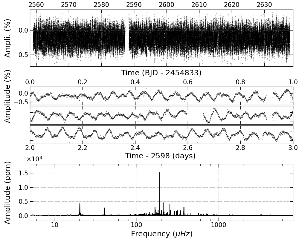
Figure 1: K2 photometry and frequency signals obtained for PG 0101+039. Top panel: Complete light curve (amplitude is in percentage, a.k.a. %, of the mean brightness) with a data sampling of 58.85 s. Middle panel: Close-up view of a 3-d light curve (starting at BJD 2457431) with each panel having a one-day slice. Bottom panel: Lomb-Scargle periodogram of the assembled light curve (amplitude in ppm vs frequency in $\mu$Hz on a logarithmic scale).

PG 0101+039 was observed by K2 in Campaign 8. As rapid oscillations in sdB pulsators, we completely downloaded the target pixel files (TPFs) in short-cadence (58.85 s) from the Mikulski Archive for Space Telescopes . The Lightkurve (Lightkurve Collaboration et al., 2018) package was used for flux extraction from the available TPFs. To complete the fine pointing during the K2 observation, a $\sim 6.5$ hr thruster firing had to be performed in order to compensate for the solar pressure variation, which led the stamp of the target to move slowly on the CCD module. We subsequently adopted the KEPSFF routine (Vanderburg & Johnson, 2014) to correct the systematic photometric variation induced by such a change in the altitude of the craft. To determine the optimal aperture, we tested a series of stamps from the TPFs (see Appendix A). The final light curves cover a duration of 78.7 days from BJD 2457392.06 to 2457470.78, as shown in the top panel of Fig 1, leaving $111{,}710$ data points. We can clearly see brightness variations with a period of around an hour from the expended light curves as shown in the middle panel of Fig 1. The Lomb-Scargle periodogram (LSP) of PG 0101+039 is demonstrated at the bottom of Fig 1, with a Nyquist frequency of approximately 8500 $\mu$Hz and significant peaks clustering around 100 to 1000 $\mu$Hz. This frequency range is suitable for detection of both p- and g-mode in sdB pulsators (Fontaine et al., 2008).

2.2 Frequency extraction and classification

Table 1: List of significant frequencies detected in PG 0101+039, by order of increasing frequency.

ID	Frequency	$\sigma$f	Period	$\sigma$P	Amplitude	$\sigma$A	S/N	$\ell$	$m$	Mode	Comments
	($\mu$Hz)	($\mu$Hz)	(s)	(s)	(ppm)	(ppm)
Frequencies in multiplets
$f_{44}$	144.0292	0.0104	6943.0373	0.5018	62.52	8.03	7.8	1	0	$g$	…
$f_{20}$	144.7187	0.0055	6909.9594	0.2630	117.88	8.01	14.7	1	1	$g$	AFM
$f_{30}$	155.3015	0.0076	6439.0879	0.3169	84.75	7.99	10.6	1	0	$g$	…
$f_{37}$	155.9591	0.0090	6411.9392	0.3690	72.00	7.97	9.0	1	1	$g$	…
$f_{7}$	167.6954	0.0021	5963.1940	0.0739	302.10	7.74	39.0	1	-1	$g$	AFM
$f_{27}$	168.4449	0.0070	5936.6595	0.2469	89.20	7.71	11.6	1	0	$g$	…
$f_{9}$	169.0794	0.0030	5914.3814	0.1045	209.27	7.71	27.1	1	1	$g$	AFM
$f_{35}$	182.5338	0.0082	5478.4369	0.2454	75.49	7.62	9.9	1	-1	$g$	…
$f_{11}$	183.1629	0.0031	5459.6210	0.0916	200.91	7.61	26.4	1	0	$g$	AFM
$f_{58}$	183.8808	0.0122	5438.3060	0.3616	50.05	7.55	6.6	1	1	$g$	…
$f_{66}$	200.5844	0.0130	4985.4327	0.3234	45.26	7.26	6.2	2	-1	$g$	…
$f_{13}$	201.6434	0.0032	4959.2499	0.0785	181.95	7.16	25.4	2	0	$g$	AFM
$f_{40}$	202.5375	0.0086	4937.3562	0.2105	67.37	7.18	9.4	2	1?	$g$	…
$f_{43}$	231.0496	0.0074	4328.0757	0.1381	64.10	5.83	11.0	2	-1	$g$	…
$f_{46}$	232.1609	0.0076	4307.3583	0.1407	61.37	5.74	10.7	2	0	$g$	AFM
$f_{64}$	234.3496	0.0096	4267.1295	0.1757	47.33	5.63	8.4	2	2	$g$	…
$f_{4}$	254.6364	0.0009	3927.1685	0.0146	404.06	4.71	85.8	1	0	$g$	S
$f_{28}$	255.2867	0.0043	3917.1639	0.0665	88.47	4.73	18.7	1	1	$g$	AFM
$f_{22}$	291.0652	0.0031	3435.6564	0.0362	101.26	3.84	26.4	1	-1	$g$	AFM
$f_{17}$	291.7374	0.0021	3427.7404	0.0244	149.76	3.83	39.1	1	0	$g$	AFM
$f_{84}$	332.1861	0.0079	3010.3603	0.0711	33.87	3.28	10.3	2	0	$g$	…
$f_{94}$	333.2654	0.0091	3000.6119	0.0822	29.11	3.28	8.9	2	1	$g$	…
$f_{103}$	334.3583	0.0107	2990.8035	0.0960	24.70	3.27	7.5	2	2	$g$	…
$f_{69}$	343.3255	0.0061	2912.6879	0.0515	42.30	3.17	13.3	1	-1	$g$	…
$f_{15}$	343.9567	0.0015	2907.3428	0.0128	169.36	3.15	53.7	$1$	$0$	$g$	AFM
$f_{6}$	377.4207	0.0008	2649.5631	0.0053	302.17	2.84	106.4	1	-1	$g$	AFM
$f_{25}$	378.0847	0.0026	2644.9102	0.0179	90.28	2.84	31.8	1	0	$g$	AFM
$f_{5}$	378.7191	0.0008	2640.4797	0.0053	305.51	2.84	107.6	1	1	$g$	AFM
$f_{111}$	450.1190	0.0091	2221.6350	0.0448	22.56	2.52	8.9	1	-1	$g$	…
$f_{24}$	450.8067	0.0021	2218.2457	0.0105	96.53	2.53	38.1	1	0	$g$	AFM
$f_{33}$	570.2222	0.0025	1753.7022	0.0077	78.16	2.41	32.4	4	-3	$g$	AFM
$f_{60}$	571.5085	0.0040	1749.7552	0.0122	49.33	2.43	20.3	4	-2	$g$	AFM
$f_{102}$	572.7683	0.0079	1745.9066	0.0240	25.13	2.44	10.3	4	-1	$g$	…
$f_{36}$	574.0246	0.0026	1742.0856	0.0079	75.38	2.43	31.0	4	0	$g$	AFM
$f_{99}$	576.5143	0.0076	1734.5624	0.0227	26.17	2.44	10.7	4	2	$g$	…
$f_{79}$	651.3998	0.0056	1535.1555	0.0132	36.24	2.51	14.4	2	-1	$g$	…
$f_{179}$	652.5496	0.0148	1532.4506	0.0348	13.83	2.53	5.5	2	0	$g$	…
$f_{50}$	653.5355	0.0036	1530.1388	0.0083	57.54	2.53	22.8	2	1	$g$	AM
$f_{87}$	702.6498	0.0063	1423.1840	0.0128	32.14	2.51	12.8	6		$g$	…
$f_{88}$	705.2075	0.0066	1418.0224	0.0133	30.93	2.53	12.2	6		$g$	…
$f_{38}$	707.7781	0.0030	1412.8722	0.0060	69.22	2.55	27.1	6—8		$g$	AFM
$f_{67}$	710.3852	0.0046	1407.6870	0.0091	45.19	2.55	17.7	8		$g$	AFM
$f_{80}$	711.7116	0.0059	1405.0636	0.0117	34.99	2.56	13.7	8		$g$	…
$f_{132}$	884.2697	0.0109	1130.8767	0.0139	19.76	2.65	7.5	$\geq 8?$		$g$	…
$f_{115}$	886.9046	0.0097	1127.5170	0.0123	22.01	2.63	8.4	$\geq 8$?		$g$	…
$f_{96}$	889.5773	0.0075	1124.1294	0.0095	28.02	2.61	10.7	$\geq 8$?		$g$	…
$f_{86}$	890.9649	0.0065	1122.3786	0.0082	32.78	2.63	12.5	$\geq 8$?		$g$	…

Table 1: continued.

ID	Frequency	$\sigma$f	Period	$\sigma$P	Amplitude	$\sigma$A	S/N	$\ell$	$m$	Mode	Comments
	($\mu$Hz)	($\mu$Hz)	(s)	(s)	(ppm)	(ppm)
$f_{128}$	929.4440	0.0103	1075.9121	0.0119	20.49	2.60	7.9	$\geq 8$?		$g$	…
$f_{172}$	933.3882	0.0146	1071.3656	0.0168	14.49	2.61	5.5	$\geq 8$?		$g$	…
$f_{164}$	934.7951	0.0142	1069.7532	0.0162	15.08	2.64	5.7	$\geq 8$?		$g$	…
$f_{136}$	1060.5123	0.0107	942.9405	0.0095	18.60	2.46	7.6	8		$g$	…
$f_{134}$	1063.1768	0.0103	940.5773	0.0091	19.34	2.45	7.9	8		$g$	…
$f_{106}$	1065.7602	0.0085	938.2973	0.0075	23.46	2.45	9.6	8		$g$	…
$f_{82}$	1367.6826	0.0060	731.1638	0.0032	34.83	2.56	13.6	4		mixed	…
$f_{107}$	1370.3923	0.0090	729.7180	0.0048	23.21	2.57	9.0	4		mixed	…
$f_{101}$	1373.1646	0.0083	728.2448	0.0044	25.15	2.59	9.7	4		mixed	…
$f_{57}$	3306.9347	0.0036	302.3948	0.0003	50.25	2.25	22.3	4		$p$	AFM
$f_{129}$	3310.7620	0.0090	302.0453	0.0008	20.33	2.26	9.0	4		$p$	…
$f_{180}$	3312.2120	0.0147	301.9130	0.0013	12.34	2.23	5.5	4		$p$	…
$f_{169}$	3313.5855	0.0123	301.7879	0.0011	14.68	2.22	6.6	4		$p$	…
Other independent frequencies
$f_{23}$	176.0551	0.0063	5680.0400	0.2049	99.85	7.82	12.8	$1^{*}$—$2^{*}$	$0^{*}$—$-2^{*}$	$g$	AFM
$f_{1}$	191.4365	0.0004	5223.6643	0.0108	1532.74	7.52	203.9	$1^{*}$—$2^{*}$	$0^{*}$—$2^{*}$	$g$	AFM
$f_{2}$	211.0751	0.0012	4737.6492	0.0264	466.68	6.77	69.0	$2^{*}$	$0^{*}$	$g$	AFM
$f_{19}$	212.3919	0.0041	4708.2776	0.0918	130.76	6.68	19.6	$1^{*}$	$0^{*}$	$g$	AFM
$f_{18}$	216.2481	0.0036	4624.3181	0.0761	146.22	6.42	22.8			$g$	AFM
$f_{21}$	238.2989	0.0040	4196.4107	0.0698	110.22	5.39	20.4	$1^{*}$	$0^{*}$	$g$	AFM
$f_{10}$	258.4635	0.0018	3869.0180	0.0273	207.41	4.67	44.4			$g$	AFM
$f_{16}$	305.5117	0.0019	3273.1966	0.0202	152.56	3.55	43.0	$2^{*}$	$-2^{*}$	$g$	AFM
$f_{12}$	314.0817	0.0015	3183.8846	0.0150	187.03	3.42	54.7	$1^{*}$	$0^{*}$	$g$	AFM
$f_{14}$	315.3790	0.0016	3170.7879	0.0159	174.72	3.41	51.3			$g$	AFM
$f_{31}$	316.7995	0.0034	3156.5707	0.0341	80.68	3.41	23.7			$g$	AFM
$f_{39}$	390.5330	0.0034	2560.6031	0.0220	67.72	2.80	24.2	$2^{*}$	$-2^{*}$	$g$	FM
$f_{41}$	414.4970	0.0033	2412.5626	0.0192	66.65	2.71	24.6	$1^{*}$	$0^{*}$	$g$	AFM
$f_{65}$	607.7807	0.0044	1645.3304	0.0120	45.86	2.51	18.3			$g$	AFM
$f_{73}$	617.1960	0.0052	1620.2307	0.0136	39.34	2.51	15.7			$g$	AFM
$f_{68}$	732.8429	0.0047	1364.5489	0.0088	44.95	2.61	17.2			$g$	AFM
$f_{85}$	3269.8990	0.0056	305.8198	0.0005	32.85	2.29	14.3			$p$	AFM
$f_{90}$	4318.7076	0.0067	231.5508	0.0004	30.30	2.52	12.0			$p$	AFM
Orbitial Information
$f_{3}$	20.3085	0.0014	49240.4255	3.4977	438.78	7.81	56.2				AFM
$f_{8}$	40.6194	0.0022	24618.7763	1.3508	272.22	7.49	36.4				AFM
Combination Frequencies
$f_{48}$	346.2998	0.0042	2887.6715	0.0354	59.60	3.12	19.1				AFM
$f_{89}$	4320.7351	0.0068	231.4421	0.0004	30.48	2.56	11.9				AFM

Computing the Fourier transforms (FT) of the light curves is helpful in examining the periodic signals presented in the data. We used the dedicated software FELIX to perform frequency extraction from the coordinated light curves. The significant frequencies were prewhitened in order of decreasing amplitude until it goes down to the adopted threshold of 5.2 times the local noise level, which is defined by the median value of the amplitude in the LSP. This signal-to-noise ratio limit of $S/N=5.2$ was adopted as a compromise between the testing results from 2-yr Kepler and 27-d TESS photometry (Zong et al., 2016b; Charpinet et al., 2019). The highest peak was meant to be extracted when several close frequencies were encompassed within $0.4\,\mu$Hz, namely, about $3\times\Delta f$, where $\Delta f=1/T$ is the frequency resolution $\sim 0.147\,\mu$Hz and T $\sim 78.7$ days. Table 1 lists 83 significant frequencies, which includes 44 frequencies whose amplitude modulations (AM) and frequency modulations (FM) are characterized in the following section. Another 39 significant frequencies were identified as rotational components, but their amplitudes were not high enough to characterize the AM or FM. The entire frequency data set is listed in Table 4, containing 137 independent frequencies, 2 orbital frequencies, and 51 linear combination frequencies. Compared to the three pulsation frequencies listed in Randall et al. (2005), the frequency around 7235 s was not detected in our list, whereas the other two were found, but with a different significant amplitude, regardless of the observation band.

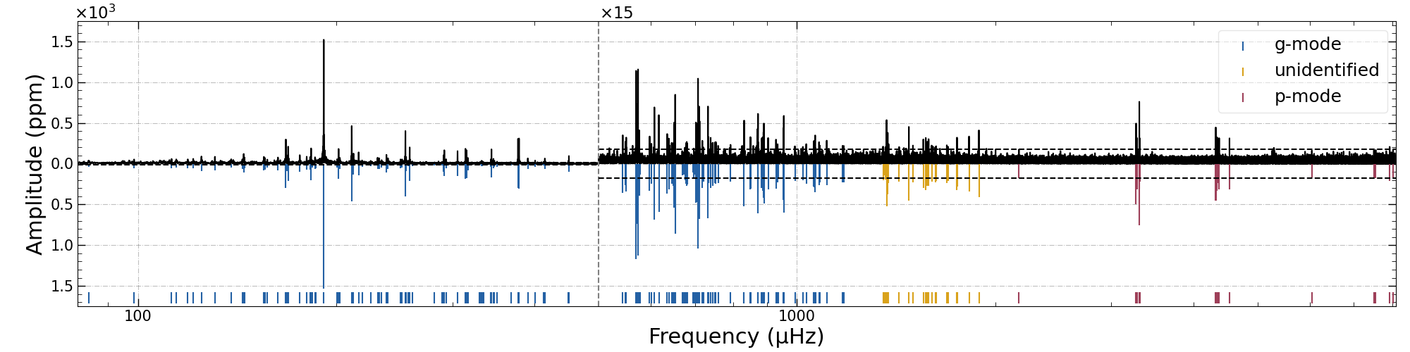
Figure 2: LSP of the K2 photometry collected on PG 0101+039, covering the frequency range where the pulsation signals are found. The entire periodogram is divided into two different ranges: the low-frequency g-mode region (blue lines) and the high-frequency p-mode region (yellow and red lines). The dashed horizontal lines are the 5.2$\sigma$ threshold of the local noise and the colorful vertical segments at the bottom of the LSP indicate the frequencies we extracted.

As rich frequencies are presented in PG 0101+039, it is wise to give a preliminary classification of acoustic p-modes and gravity g-modes, since their seismic properties are different. We followed a similar treatment of this classification to Ma et al. (2022), barely by their pulsation period. Theoretical calculations of sdB pulsators suggest that dipole p-modes typically exhibit periods of $<400$ s (or $f>2500\,\mu$Hz), whereas their g-modes are $>1000$ s (or $f<1000\,\mu$Hz) (see, e.g., Fontaine et al., 2003; Charpinet et al., 2005, 2011b). However, p-mode periods can increase beyond 600 s when $T_{\mathrm{eff}}$ and $\log g$ decreases (Charpinet, 1999; Charpinet et al., 2001, 2002a). This brings on difficulties in terms of the direct classification of p- and g-mode when their periods are around 600 s, even though PG 0101+039 is clearly located in the g-mode dominating pulsator. Figure 2 shows the part of the LSP where the pulsation frequencies are extracted and labeled with preliminary classification. We detected 94 independent frequencies in the range of [$\sim 80-1200$] $\mu$Hz that are highly probable g-modes (the blue vertical segments). Another 16 independent frequencies were found in the high-frequency p-mode region, [$\sim 2600-8000$] $\mu$Hz (the red vertical segments); there are another 9 independent frequencies in the region of [$\sim 1200-2000$] $\mu$Hz (the yellow segments), which might be low-order high-degree ( $\ell>3$) g-modes or mixed modes. This latter assumption requires further classification (see, e.g., Charpinet et al., 2011b, 2019). In addition, within the frequency range of 1200 and 2000 $\mu$Hz, we resolved ten linear combinations that could be intrinsic resonant modes (Zong et al., 2016a) or nonlinear effects from the linear eigenfrequencies (Brassard et al., 1995). In the following, we discuss a more sophisticated determination of quantum numbers of those pulsation modes by their seismic properties.

2.3 Rotational multiplets

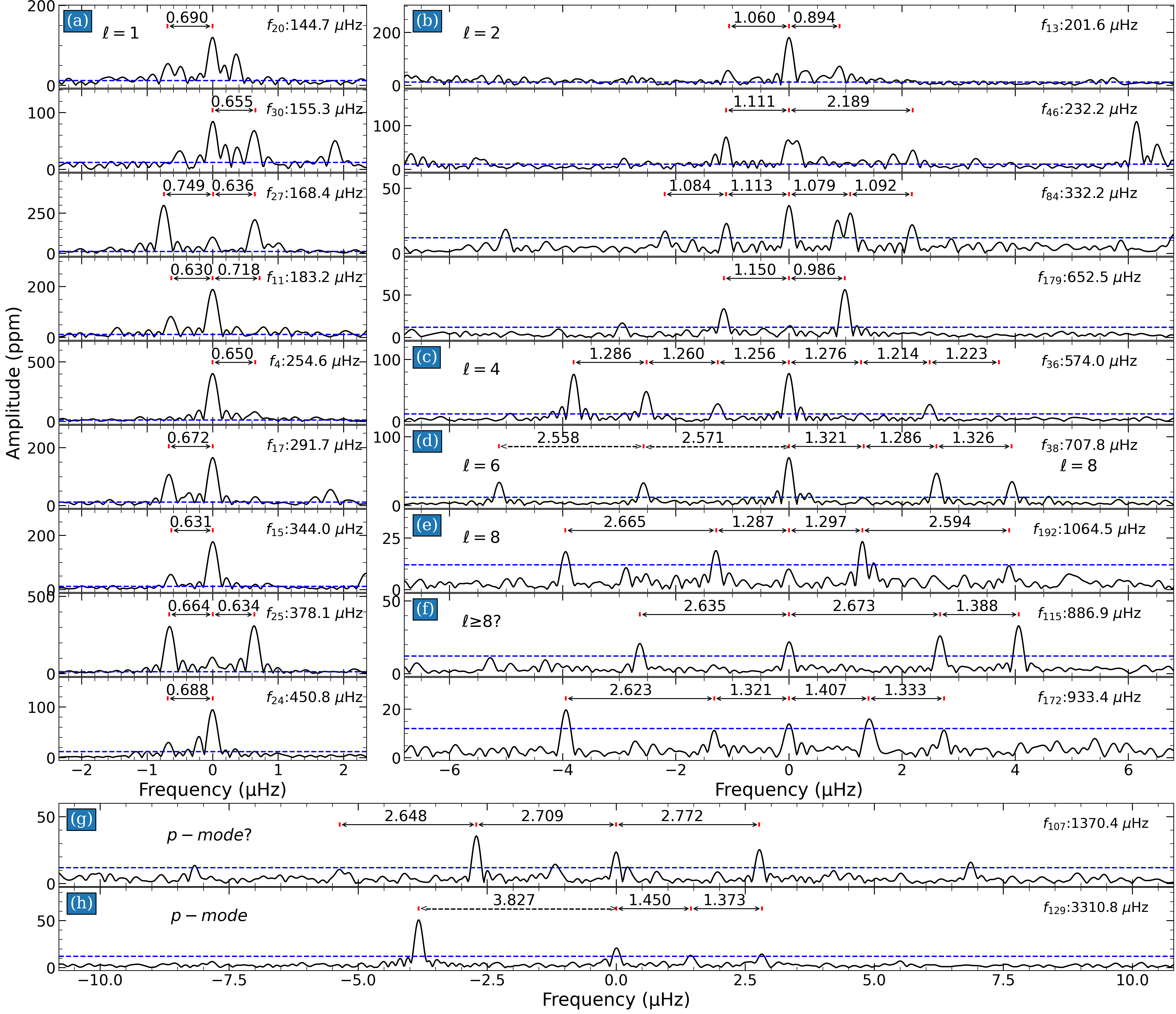
Figure 3: Rotational multiplets identified in PG 0101+039 by the common frequency spacing. All the components, labeled by vertical segments, are shifted to the frequencies as given in the text. The value of splitting is given in the text and indicated by the annotation of double arrows between the segments, whereas two types of arrow lines indicate the different interpretations of rotation multiplets (see text for details). The blue horizontal lines are the $5.2\sigma$ detection threshold. (a)-(e) Different degree $\ell$ multiplets in g-mode region, (f) suspected high degree multiplets with $\ell\geq 8$ in g-mode region, (g) mixed mode region to be identified of p-modes? and (h) p-mode region.

When a star rotates slowly, the non-radial degenerate frequencies will be split into $2\ell+1$ components. According to the first order of approximation of the effect of rigid rotation treated on a perturbation, the frequencies of the components follow the formulae (Dziembowski & Goode, 1992):

$$\nu_{n,l,m}=\nu_{n,l,0}+m\Omega(1-C_{n,\ell}),$$ (1)

where $\nu_{n,l,0}$ is the frequency of the central ($m=0$) component, $\Omega$ is the solid rotational frequency, and the Ledoux constant, $C_{n,\ell}\ll 1,$ is valid for acoustic p-mode and $C_{n,\ell}\sim 1/\ell(\ell+1)$ for high-radial order gravity g-mode. According to the frequency spacing of rotational multiplets, it is helpful to determine the rotation period and give precise identification of oscillation modes in pulsating stars.

In PG 0101+039, we detected a common frequency spacing of $\sim 0.6-1.3\,\mu$Hz, as per the frequencies listed in Table 1. In Fig. 3, we present all the groups of rotational components identified by frequency spacing. In the low-frequency g-mode region, we detected nine groups of frequency spacing of $\sim 0.66\,\mu$Hz, from $0.63$ to $0.75\,\mu$Hz, i.e., $f_{20}\sim$ 144.72 $\mu$Hz, $f_{30}\sim$ 155.30 $\mu$Hz, $f_{27}\sim$ 168.44 $\mu$Hz, $f_{11}\sim$ 183.16 $\mu$Hz, $f_{4}\sim$ 254.64 $\mu$Hz, $f_{17}\sim$ 291.74 $\mu$Hz, $f_{15}\sim$ 343.96 $\mu$Hz, $f_{25}\sim$ 378.08 $\mu$Hz, and $f_{24}\sim$ 450.80 $\mu$Hz, including three triplets and six doublets with one missing component. We note that the worst precision of frequency in those components is around $0.02\,\mu$Hz. We interpreted the frequency spacing of $\sim{0.66}\,\mu$Hz as being the minimum common spacing for dipole mode rotation, since frequency spacing increases with the degree $\ell$. According to Eq. 1, the frequency spacings of $\ell=2,4,6,8$ are 1.10 $\mu$Hz, 1.26 $\mu$Hz, 1.29 $\mu$Hz, and 1.30 $\mu$Hz, respectively. Roughly considering that $C_{n,1}=1/2$, we can deduce a rotation period of $P=8.75\pm 0.13$ d from the weighted average value $\Delta\nu=0.66\pm 0.01\leavevmode\nobreak\ \mu$Hz based on the above nine triplets (where the weight is set according to their S/N). We also found four groups of frequencies that can be associated with quadrupole modes with frequency spacing of $\sim 1.08\,\mu$Hz, namely, $f_{13}\sim$ 201.64 $\mu$Hz, $f_{46}\sim$ 232.16 $\mu$Hz, $f_{84}\sim$ 332.18 $\mu$Hz, and $f_{179}\sim$ 652.55 $\mu$Hz including one full quintuplet and three incomplete ones. Similarly to $\ell=1$ (but considering $C_{n,2}=1/6$), the rotation period can be derived to be $P=8.78\pm 0.10$ d from the above four quintuplets. Thus, both the $\ell=1$ and $\ell=2$ modes suggest that the rotation period should be around 8.8 days.

With the rotation period known, we can further identify with high confidence several high-degree ($\ell>3$) frequencies in the g-mode region. With a frequency spacing of $\sim 1.26\pm 0.01\,\mu$Hz, the five significant frequencies and two suspected ones around $f_{36}\sim$ 574.03 $\mu$Hz would correspond to an $\ell=4$ multiplet with two missing components, since the $\ell=4$ modes should exhibit a frequency splitting of $1.26\,\mu$Hz according to Eq. 1. If we only count the five significant frequencies, the splitting has the same value, which still satisfies the $\ell=4$ identification. We note that the $\ell=5$ modes with $\Delta\nu\sim 1.27\,\mu$Hz could meet the measured splitting too, but high odd-degree modes suffer a much higher geometric cancellation effect (Aerts et al., 2010). We thus do not consider any high odd-degree modes in PG 0101+039 anymore and classified the frequency group around $f_{36}\sim$ 574.03 $\mu$Hz as an $\ell=4$ multiplet. The frequency spacing found around $f_{38}\sim 707.78\,\mu$Hz shows a distinct feature, namely, the most left and right three components can be derived with $\sim 1.28\,\mu$Hz and $\sim 1.31\,\mu$Hz, respectively. One explanation is that they belong to two different multiplets with $\ell=6$ ($\Delta\nu\sim 1.283\pm 0.003\,\mu$Hz) and $\ell=8$ ($\Delta\nu\sim 1.314\pm 0.012\,\mu$Hz), respectively. Otherwise, we measured an average frequency splitting of $\sim 1.30\pm 0.01\,\mu$Hz from all six components, which could be attributed to an $\ell=8$ multiplet. One clearly incomplete $\ell=8$ multiplet is probably found around $f_{134}\sim 1063.17\,\mu$Hz, where five components were identified by a frequency spacing of $\Delta\nu\sim 1.30\,\mu$Hz. We also detected two incomplete multiplets near $f_{115}\sim 886.90\,\mu$Hz and $f_{172}\sim 933.38\,\mu$Hz, possibly having a degree of $\ell\geq 8$, based on a frequency spacing of $\Delta\nu\sim 1.34\pm 0.01\,\mu$Hz. If we exclude the two relatively large spacing with $\Delta\nu=1.404$ and $1.388\leavevmode\nobreak\ \mu$Hz in $f_{172}$ and $f_{115}$, respectively, the frequency spacing is $\sim 1.325\pm 0.005\,\mu$Hz; this value is close to the $\ell=8$ splitting. We recall here that a high even-degree, for instance, $\ell=12,14,\cdots$, can also satisfy the splitting of $\Delta\nu\sim 1.32\,\mu$Hz but the geometric cancellation effect increases with the value of $\ell$. Thus, it is wise to keep $\ell$ at the minimum value.

For the multiplets above the low-frequency g-modes, we give the preliminary identification of degree number as the Ledoux constant $C_{n,l}$ is near to 0 for p-modes. In the mixed region near $f_{107}\sim 1370.39\,\mu$Hz, the frequency spacing is derived to be $1.355\pm 0.017\,\mu$Hz if we count all three significant frequencies and one suspected frequency of $f_{190}^{*}\sim 1365.03\,\mu$Hz. This measurement may be a bit larger, namely, $\sim 1.37\,\mu$Hz, when derived from only the three significant frequencies. Whether this multiplet is high degree g-modes or p-modes, this splitting is somewhat larger than the previous multiplets with a rational frequency splitting of $\sim 1.315\,\mu$Hz. We prefer this multiplet to be in p-modes, in line with a similar frequency splitting found in the p-mode multiplet around $\sim 3310.8\,\mu$Hz. We measured a frequency spacing of $\sim 1.34\,\mu$Hz for all four components or $\sim 1.41\,\mu$Hz for the rightmost three components around $f_{129}\sim 3310.8\,\mu$Hz. Consistently with the chosen minimum degree number, the preliminary classifications are both $\ell=4$ for the multiplets around $1370.4\,\mu$Hz and $3310.8\,\mu$Hz. It would be very surprising to find that both two multiplets are identified with degrees, not of $\ell=1$ or 2. The low-degree modes seem to have a higher chance of being observed. To reman cautious, these p-mode multiplets may also be mixed with dipole or quadrupole modes if we discard the frequencies with an amplitude of S/N$<5.2$. However, to give an exact discriminant mode, it is necessary to wait for the future seismic model on PG 0101+039.

Finally, we note that the frequency spacing between different components within the same multiplet may display a frequency mismatch up to $0.1\,\mu$Hz, for instance, with respect to the triplet of $f_{7}\sim 168\,\mu$Hz. This is not a defect in rotational components considering the measuring uncertainty and variation of frequency. In general, the frequency variation is $\sim 1.6\times$ the frequency mismatch, even though the measuring uncertainty is merely 17% of the frequency mismatch. Therefore, we derived a rotational period of $\sim 8.81\pm 0.06$ days based on the weighted average splitting from the 14 g-mode multiplets (see Fig. 3 a-e). With the two p-mode multiplets (Fig. 3, g-h), we derived a rotational period of $8.60\pm 0.16$ days, which is slightly faster than that of the g-modes. Our result suggests that PG 0101+039 has a differential rotation with a faster rotating envelope than the core. To remain cautious, we assume that PG 0101+039 may still be a rigid object with a probability up to $\sim 40\%$ if the uncertainties of rotational periods are fully considered. Moreover, we also tried to analyze the period spacing of g-modes in PG 0101+039, but without any clear-cut patterns found (see Appendix C for details).

3 Amplitude and frequency modulations

This section is devoted to characterizing amplitude modulation (AM) and frequency modulation (FM) occurring in significant frequencies with high-enough amplitudes. Recent studies indicate that most oscillation modes are unstable in pulsating sdB stars (see, e.g., Zong et al., 2016a; Ma et al., 2022). To obtain enough amplitude and frequency measuring points, we have to choose the frequencies with $\rm{S/N}>8.8$ for our aims. The frequency and amplitude errors derived from Felix had been estimated by Zong et al. (2016a) and Zong et al. (2021), whose results demonstrate that those errors are well determined and robust. In PG 0101+039, there are 44 frequencies that met this criterion, including 19 rotational components. After comparing the results of AM and FM from photometry that are extracted via stamps with various pixels (see Appendix D for details), the AMs and FMs were characterized (as given in Sections 3.1 and 3.2).

As supported by the comparing results in Appendix D, we ultimately selected a conservative stamp ($N=16$) for measuring AMs and FMs of 44 frequencies that are commented in the last column of Table 1. As proposed in the previous work by Ma et al. (2022), the modulating patterns of AMs and FMs can be quantitatively characterized with several simple fitting functions. Here, we follow the same strategy and characterize the discovered AMs and FMs occurring in PG 0101+039, via the linear combinations of three simple types of fittings (linear, parabolic, and sinusoidal waves), as defined by a matrix function of:

$$G_{k}(t)=\left[g_{1}(t),g_{2}(t),g_{3}(t),g_{1}(t)+g_{3}(t),g_{2}(t)+g_{3}(t)\right],$$ (2)

$$\left\{\begin{array}[]{l}g_{1}(t)=bt+c,\\ g_{2}(t)=at^{2}+bt+c,\\ g_{3}(t)=A\sin(\omega t+\phi)+A_{0},\end{array}\right.$$

where $k=1,2,3,4,5$. We finally chose the fitting function by increasing the index of $k$ after a quantitative evaluation. Then the Markov chain Monte Carlo (MCMC) method was applied to derive the uncertainties for the optimal fittings. MCMC is implemented by the EMCEE code (Foreman-Mackey et al., 2013) and sample posterior distributions of parameters. We can see the detailed processes for such analysis in Sect. 3 of Ma et al. (2022). Table 2 lists the information of each fitting function for the 45 frequencies with AM and FM, including the fitting coefficients and the correlation between AM and FM.

Figure 4 is a gallery composed of eight portraits that depict AM and FM of each frequency through various fitting functions, $G_{k}(t)$. Except for the modulating patterns of $f_{4}\sim 254.6\,\mu$Hz, they clearly exhibit evident AM and FM in various patterns, with a majority of them containing a sinusoidal component. Most of those frequencies and amplitudes have undergone an oscillatory behavior back and forth around their average values, for instance, modulations of $f_{44}\sim 414.5\,\mu$Hz fitted with $G_{4}$ containing a slight linear trend. However, two frequencies, $f_{23}\sim 176.1\,\mu$Hz and $f_{46}\sim 232.1\,\mu$Hz, show a significant linear decreasing and increasing trend, which makes them detectable in only half of the observation. We note that some correlation or anti-correlation happens between the AMs and FMs, for instance, a significant anti-phase of $\rho_{\mathrm{am,fm}}=-0.82$ is derived for $f_{44}\sim 414.5\,\mu$Hz.

3.1 AM and FM in Multiplets

In this subsection, we focus on the AMs and FMs occurring in five multiplets as themselves are under the resonant condition, including one triplet near 377 $\mu$Hz (Fig. 5), two doublets near 167 $\mu$Hz and 291 $\mu$Hz (Fig. 6 and 13), one incomplete $\ell=4$ multiplet near 570 $\mu$Hz (Fig. 14), and one multiplet possibly containing $\ell=6$ and $\ell=8$ components near 707 $\mu$Hz (Fig. 15). Here, we describe the details of AMs and FMs occurring in the complete triplet near 377 $\mu$Hz and one doublet near 167 $\mu$Hz. For simplicity, the detailed behaviors of AMs and FMs of the other mentioned multiplets are given in Appendix E.1.

Table 2: AM/FM detected in PG 0101+039, sorted by order of increasing frequency.

ID	Fre	Corr	AM/FM	A	T=2 $\pi$/$\omega$	$\phi$	a	b	c	Fitting
	($\mu$Hz)			(ppm/nHz)	(d)	[0, 2$\pi$)	(10-3)	(10-2)
AFMs in multiplets
$f_{7}$	167.6896	0.34	AM	–	–	–	${29_{-4}^{+4}}$	${226_{-16}^{+16}}$	${271_{-2}^{+2}}$	$G_{2}$
			FM	$12.7_{-1.2}^{+1.2}$	$16.8_{-0.3}^{+0.3}$	$3.8_{-0.2}^{+0.2}$	–	$-13_{-6}^{+7}$	${3.3_{-1.7}^{+1.7}}$	$G_{4}$
$f_{9}$	$169.0805$	$0.33$	AM	$38.5_{-1.7}^{+1.7}$	$29.1_{-0.4}^{+0.4}$	$1.8_{-0.1}^{+0.1}$	–	$150_{-10}^{+10}$	$-30.6_{-2.7}^{+2.6}$	$G_{4}$
			FM	$17.0_{-1.6}^{+1.6}$	$18.9_{-0.3}^{+0.3}$	$2.6_{-0.2}^{+0.2}$	–	$70_{-10}^{+10}$	$204_{-2}^{+2}$	$G_{4}$
$f_{22}$	291.0679	$0.62$	AM	$8.9_{-1.5}^{+1.5}$	$41.2_{-3.5}^{+3.9}$	$2.9_{-0.4}^{+0.3}$	–	$6_{-12}^{+12}$	$104_{-3}^{+3}$	$G_{4}$
			FM	$31.4_{-2.0}^{+2.0}$	$39.2_{-1.4}^{+1.3}$	$4.3_{-0.2}^{+0.2}$	–	$-11_{-16}^{+16}$	$0.19_{-4.14}^{+4.10}$	$G_{4}$
$f_{17}$	291.7364	-0.13	AM	$4.8_{-0.8}^{+0.8}$	$33.9_{-2.5}^{+2.9}$	$1.14_{-0.35}^{+0.36}$	–	$-8_{-6}^{+6}$	$151_{-1}^{+1}$	$G_{4}$
			FM	$20.4_{-1.2}^{+1.3}$	$26.8_{-0.4}^{+0.4}$	$2.7_{-0.1}^{+0.1}$	–	$15_{-8}^{+8}$	$-5.3_{-1.7}^{+1.7}$	$G_{4}$
$f_{6}$	377.4208	0.49	AM	–	–	–	$-18_{-1}^{+1}$	$77_{-4}^{+5}$	$297_{-1}^{+1}$	$G_{2}$
			FM	$2.7_{-0.4}^{+0.4}$	$35.7_{-2.2}^{+2.5}$	$1.1_{-0.3}^{+0.3}$	–	$-4_{-3}^{+3}$	$1.36_{-0.65}^{+0.63}$	$G_{4}$
$f_{25}$	378.0836	$0.26$	AM	$2.5_{-0.3}^{+0.3}$	$13.0_{-0.2}^{+0.2}$	$0.15_{-0.21}^{+0.21}$	–	$-24_{-3}^{+3}$	$96.8_{-0.4}^{+0.4}$	$G_{4}$
			FM	$12.9_{-1.6}^{+1.6}$	$27.1_{-0.8}^{+0.8}$	$5.1_{-0.2}^{+0.2}$	–	$-1_{-10}^{+10}$	$1.6_{-2.1}^{+2.1}$	$G_{4}$
$f_{5}$	378.7156	-0.51	AM	$15.5_{-1.6}^{+1.6}$	$60.1_{-3.0}^{+3.2}$	$60_{-3}^{+3}$	–	$13_{-10}^{+10}$	$298_{-2}^{+2}$	$G_{4}$
			FM	$3.8_{-0.3}^{+0.3}$	$28.8_{-0.6}^{+0.7}$	$5.6_{-0.1}^{+0.1}$	–	$40_{-3}^{+3}$	$-10.0_{-0.5}^{+0.5}$	$G_{4}$
$f_{33}$	$570.2229$	-0.07	AM	–	–	–	$14_{-1}^{+1}$	$-59_{-5}^{+5}$	$79_{-1}^{+1}$	$G_{2}$
			FM	$9.7_{-1.3}^{+1.3}$	$31.2_{-1.3}^{+1.4}$	$5.4_{-0.2}^{+0.2}$	–	$-40_{-9}^{+8}$	$8.0_{-1.9}^{+1.9}$	$G_{4}$
$f_{60}$	$571.5070$	-0.48	AM	–	–	–	$-14_{-1}^{+1}$	$72_{-4}^{+4}$	$45.8_{-0.5}^{+0.5}$	$G_{2}$
			FM	–	–	–	–	$-87_{-9}^{+9}$	$20.3_{-2.4}^{+2.3}$	$G_{1}$
$f_{36}$	$574.0266$	0.53	AM	$1.85_{-0.25}^{+0.26}$	$8.8_{-0.1}^{+0.1}$	$1.65_{-0.26}^{+0.26}$	$10_{-1}^{+1}$	$-60_{-4}^{+4}$	$82.7_{-0.5}^{+0.5}$	$G_{5}$
			FM	$5.3_{-1.1}^{+1.1}$	$26.8_{-1.6}^{+1.8}$	$3.9_{-0.4}^{+0.4}$	–	$-34_{-8}^{+8}$	$8.2_{-1.5}^{+1.5}$	$G_{4}$
$f_{38}$	$707.7771$	-0.49	AM	$5.2_{-0.7}^{+0.8}$	$51.7_{-3.7}^{+4.2}$	$2.2_{-0.2}^{+0.2}$	–	–	$70.6_{-1.1}^{+1.1}$	$G_{3}$
			FM	$11.3_{-1.5}^{+1.5}$	$32.2_{-1.3}^{+1.3}$	$-2.9_{-0.2}^{+0.2}$	–	$14_{-1}^{+1}$	$-1.2_{-2.0}^{+2.0}$	$G_{4}$
$f_{67}$	$710.3810$	0.20	AM	–	–	–	–	$1_{-1}^{+1}$	$45.6_{-0.4}^{+0.6}$	$G_{1}$
			FM	$17_{-2}^{+2}$	$29.8_{-0.1.0}^{+0.9}$	$-3.4_{-0.2}^{+0.2}$	–	$78_{-14}^{+14}$	$-13.8_{-2.7}^{+2.7}$	$G_{4}$
Other AFMs
$f_{20}$	$144.7211$	$0.3$	AM	$6_{-1}^{+1}$	$15.3_{-0.4}^{+0.5}$	$5.5_{-0.3}^{+0.3}$	–	$20_{-10}^{+10}$	$110_{-2}^{+2}$	$G_{4}$
			FM	$52^{+3}_{-3}$	$27.5^{+0.4}_{-0.4}$	$2.4^{+0.1}_{-0.1}$	–	$230^{+20}_{-20}$	$-52^{+4}_{-4}$	$G_{4}$
$f_{23}$	$176.0526$	$0.72$	AM	–	–	–	–	$-205_{-8}^{+8}$	$158.7_{-1.3}^{+1.4}$	$G_{1}$
			FM	$33.0_{-2.4}^{+2.3}$	$19.9_{-0.4}^{+0.5}$	$-2.7_{-0.12}^{+0.12}$	–	$-290_{-20}^{+20}$	$-48.7_{-2.9}^{+3.0}$	$G_{4}$
$f_{11}$	$183.1638$	-0.13	AM	$10_{-1}^{+1}$	$17.9_{-0.3}^{+0.3}$	$3.7_{-0.2}^{+0.2}$	$-46_{-3}^{+3}$	$270_{-10}^{+10}$	$181_{-2}^{+2}$	$G_{5}$
			FM	$28_{-1}^{+1}$	$17.3_{-0.1}^{+0.1}$	$6.1_{-0.1}^{+0.1}$	$-74_{-3}^{+4}$	$340_{-20}^{+20}$	$-27_{-2}^{+2}$	$G_{5}$
$f_{1}$	191.4365	0.12	AM	$8.2_{-1.2}^{+1.3}$	$13.9_{-0.3}^{+0.3}$	$1.7_{-0.3}^{+0.3}$	$68_{-4}^{+4}$	$-460_{-20}^{+20}$	$1577_{-2}^{+2}$	$G_{4}$
			FM	–	–	–	–	–	–	–
$f_{13}$	201.6427	0.62	AM	–	–	–	–	–	–	–
			FM	$51_{-2}^{+2}$	$39_{-1}^{+1}$	$5.1_{-0.1}^{+0.1}$	–	$38_{-17}^{+17}$	$-4.9_{-4.7}^{+4.5}$	$G_{4}$
$f_{2}$	211.0748	-0.03	AM	–	–	–	–	$-31_{-3}^{+3}$	$476_{-1}^{+1}$	$G_{1}$
			FM	$2.9_{-0.5}^{+0.5}$	$30.1_{-1.6}^{+1.9}$	$5.1_{-0.3}^{+0.3}$	–	$-1.2_{-3.2}^{+3.2}$	$0.6_{-0.7}^{+0.7}$	$G_{4}$
$f_{19}$	212.3933	$0.53$	AM	$5.5_{-0.9}^{+0.9}$	$23.8_{-0.8}^{+0.9}$	$6.1_{-0.3}^{+0.3}$	–	$44_{-6}^{+6}$	$124_{-1}^{+1}$	$G_{4}$
			FM	$19.2_{-2.5}^{+2.5}$	$39_{-3}^{+3}$	$5.2_{-0.3}^{+0.3}$	–	$25_{-19.9}^{+18.8}$	$-1.4_{-4.9}^{+5.1}$	$G_{4}$
$f_{18}$	216.2493	0.75	AM	–	–	–	$-100_{-3}^{+3}$	$300_{-10}^{+10}$	$163_{-1}^{+1}$	$G_{2}$
			FM	–	–	–	$-120_{-6}^{+6}$	$510_{-30}^{+30}$	$-31_{-3}^{+3}$	$G_{2}$
$f_{46}$	232.1455	0.45	AM	–	–	–	–	$167_{-14}^{+14}$	$91.7_{-1.8}^{+1.7}$	$G_{1}$
			FM	$21_{-2}^{+2}$	$9.9_{-0.2}^{+0.2}$	$0.45_{-0.18}^{+0.19}$	–	$120_{-30}^{+30}$	$-13_{-3}^{+3}$	$G_{4}$
$f_{21}$	238.3032	$0.06$	AM	–	–	–	–	$15_{-4}^{+3}$	$104_{-1}^{+1}$	$G_{1}$
			FM	$38_{-2}^{+2}$	$30.4_{-0.5}^{+0.6}$	$1.1_{-0.1}^{+0.1}$	–	–	–	$G_{3}$

Table 2: continued.

ID	Fre	Corr	AM/FM	A	T=2 $\pi$/$\omega$	$\phi$	a	b	c	Fitting
	($\mu$Hz)			(ppm/nHz)	(d)	[0, 2$\pi$)	(10-3)	(10-2)
$f_{4}$	254.6373	$0.12$	AM	–	–	–	–	$-2_{-3}^{+4}$	$404_{-1}^{+1}$	$G_{1}$
			FM	–	–	–	–	$0.6_{-2.4}^{+2.4}$	$-0.17_{-0.64}^{+0.67}$	$G_{1}$
$f_{28}$	255.2858	$0.33$	AM	$4.4_{-0.5}^{+0.6}$	$20.1_{-0.6}^{+0.6}$	$1.87_{-0.23}^{+0.23}$	–	$-16_{-5}^{+5}$	$93.6_{-0.8}^{+0.8}$	$G_{4}$
			FM	$13.1_{-2.6}^{+2.5}$	$16.2_{-0.5}^{+0.5}$	$4.1_{-0.3}^{+0.3}$	–	$-41_{-14}^{+15}$	$9.7_{-3.4}^{+3.4}$	$G_{4}$
$f_{10}$	258.4617	$-0.53$	AM	–	–	–	–	$12_{-3}^{+3}$	$206_{-1}^{+1}$	$G_{1}$
			FM	$7.3_{-1.2}^{+1.2}$	$37.2_{-3.1}^{+3.7}$	$5.8_{-0.4}^{+0.4}$	–	$-10_{-10}^{+10}$	$1.9_{-2.4}^{+2.4}$	$G_{4}$
$f_{16}$	305.5128	0.4	AM	–	–	–	–	$62.9_{-2.8}^{+2.7}$	$140_{-1}^{+1}$	$G_{1}$
			FM	–	–	–	$39_{-3}^{+4}$	$-140_{-20}^{+20}$	$4.4_{-2.0}^{+2.0}$	$G_{2}$
$f_{12}$	314.0823	$-0.05$	AM	$4.3_{-0.4}^{+0.4}$	$23.0_{-0.5}^{+0.6}$	$4.2_{-0.2}^{+0.2}$	–	$14_{-4}^{+4}$	$181_{-1}^{+1}$	$G_{4}$
			FM	–	–	–	$-25_{-3}^{+3}$	$140_{-10}^{+10}$	$-13.7_{-1.5}^{+1.5}$	$G_{2}$
$f_{14}$	315.3790	$0.95$	AM	$24.1_{-2.5}^{+2.7}$	$59.8_{-2.9}^{+3.0}$	$2.67_{-0.13}^{+0.13}$	–	$25_{-13}^{+12}$	$170.5_{-3.9}^{+4.1}$	$G_{4}$
			FM	$20.4_{-1.5}^{+1.6}$	$36.6_{-2.1}^{+2.2}$	$0.86_{-0.2}^{+0.2}$	–	$170_{-20}^{+20}$	$-38.7_{-3.8}^{+3.9}$	$G_{4}$
$f_{31}$	$316.7981$	-0.28	AM	–	–	–	–	$-15_{-2}^{+2}$	$87.0_{-0.5}^{+0.5}$	$G_{1}$
			FM	$6.4_{-2.4}^{+2.3}$	$17_{-1}^{+1}$	$0.05_{-0.51}^{+0.53}$	–	$26_{-13}^{+13}$	$-6.5_{-3.0}^{+3.0}$	$G_{4}$
$f_{15}$	343.9562	-0.46	AM	$8.9_{-0.6}^{+0.6}$	$18.7_{-0.2}^{+0.2}$	$0.52_{-0.12}^{+0.12}$	–	$-24_{-4}^{+4}$	$178_{-1}^{+1}$	$G_{4}$
			FM	$12.7_{-1.0}^{+1.0}$	$21.2_{-0.3}^{+0.4}$	$1.7_{-0.2}^{+0.2}$	–	$-44_{-6}^{+6}$	$9.4_{-1.4}^{+1.4}$	$G_{4}$
$f_{39}$	390.5333	-0.06	AM	$1.8_{-0.3}^{+0.3}$	$18.4_{-0.7}^{+0.8}$	$2.2_{-0.4}^{+0.4}$	–	$-6_{-4}^{+4}$	$66.1_{-0.6}^{+0.6}$	$G_{4}$
			FM	$9.8_{-1.3}^{+1.3}$	$33.7_{-1.6}^{+1.8}$	$0.46_{-0.24}^{+0.25}$	–	$-90_{-10}^{+10}$	$18.7_{-1.8}^{+1.8}$	$G_{4}$
$f_{41}$	414.4996	-0.82	AM	$6.5_{-0.3}^{+0.3}$	$24.5_{-0.3}^{+0.3}$	$5.2_{-0.1}^{+0.1}$	–	$-9_{-3}^{+3}$	$67.7_{-0.4}^{+0.4}$	$G_{4}$
			FM	$40_{-2}^{+2}$	$26.2_{-0.3}^{+0.3}$	$5.6_{-0.1}^{+0.1}$	–	$10_{-12}^{+12}$	$1.0_{-2.7}^{+2.6}$	$G_{4}$
$f_{24}$	450.8051	$-0.88$	AM	$3.8_{-0.3}^{+0.3}$	$20.3_{-0.3}^{+0.3}$	$3.80_{-0.13}^{+0.14}$	$55_{-1}^{+1}$	$-292_{-4}^{+4}$	$118_{-1}^{+1}$	$G_{5}$
			FM	$14.0_{-1.3}^{+1.3}$	$18.0_{-0.3}^{+0.3}$	$0.20_{-0.15}^{+0.15}$	$-112_{-4}^{+4}$	$560_{-20}^{+20}$	$-50_{-2}^{+2}$	$G_{5}$
$f_{65}$	$607.7826$	0.74	AM	–	–	–	$-19_{-1}^{+1}$	$90_{-4}^{+4}$	$42.4_{-0.6}^{+0.6}$	$G_{2}$
			FM	–	–	–	$-86_{-6}^{+6}$	$450_{-26}^{+26}$	$-42_{-3}^{+3}$	$G_{2}$
$f_{73}$	$617.1965$	-0.42	AM	$1.5_{-0.3}^{+0.3}$	$29.3_{-2.3}^{+2.5}$	$-0.2_{-0.3}^{+0.3}$	–	$-13_{-5}^{+5}$	$45.1_{-0.4}^{+0.4}$	$G_{4}$
			FM	$9.3_{-1.8}^{+01.8}$	$20.3_{-1.2}^{+1.4}$	$-0.98_{-0.34}^{+0.36}$	–	$130_{-20}^{+20}$	$-19.5_{-2.5}^{+2.5}$	$G_{4}$
$f_{50}$	$653.5360$	$-0.32$	AM	$1.6^{+0.4}_{-0.4}$	$11.8_{-0.16}^{+0.29}$	$0.75_{-0.43}^{+0.45}$	–	$11_{-3}^{+3}$	$56.2_{-0.6}^{+0.6}$	$G_{4}$
			FM	–	–	–	–	$-18_{-7}^{+7}$	$4.2_{-1.9}^{+2.0}$	$G_{1}$
$f_{68}$	$732.8429$	0.30	AM	$1.2_{-0.3}^{+0.3}$	$29.3_{-2.3}^{+2.9}$	$-1.8_{-0.6}^{+0.6}$	–	$12_{-3}^{+3}$	$42.6_{-0.5}^{+0.5}$	$G_{4}$
			FM	–	–	–	$75_{-10}^{+9}$	$-390_{-50}^{+50}$	$40_{-7}^{+7}$	$G_{2}$
$f_{85}$	$3269.8987$	-0.79	AM	–	–	–	–	$-45_{-1}^{+1}$	$45.8_{-0.2}^{+0.2}$	$G_{1}$
			FM	$6.2_{-1.5}^{+1.4}$	$9.5_{-0.4}^{+0.4}$	$-0.2_{-0.4}^{+0.4}$	–	$110_{-20}^{+20}$	$-17_{-2}^{+2}$	$G_{4}$
$f_{57}$	$3306.9341$	-0.18	AM	$4.1_{-0.2}^{+0.2}$	$44.6_{-1.4}^{+1.5}$	$4.97_{-0.12}^{+0.12}$	–	$-43_{-2}^{+2}$	$63.2_{-0.4}^{+0.4}$	$G_{4}$
			FM	$21.3_{-10.6}^{+16.1}$	$69.0_{-19.7}^{+33.9}$	$0.35_{-0.92}^{+0.75}$	–	$120_{-50}^{+70}$	$-34.5_{-21.1}^{+16.6}$	$G_{4}$
$f_{90}$	$4318.7053$	0.49	AM	–	–	–	$58_{-9}^{+9}$	$250_{-15}^{+16}$	$30.9_{-0.9}^{+0.9}$	$G_{2}$
			FM	–	–	–	$539_{-43}^{+44}$	$1150_{-80}^{+80}$	$-43.0_{-4.6}^{+4.6}$	$G_{2}$
Combination frequencies
$f_{48}$	$346.4111$	-0.32	AM	–	–	–	–	$25_{-2}^{+2}$	$54_{-1}^{+1}$	$G_{1}$
			FM	$25_{-2}^{+2}$	$10.5_{-0.1}^{+0.1}$	$1.5_{-0.2}^{+0.2}$	–	$-71_{-13}^{+13}$	$15.7_{-2.9}^{+2.9}$	$G_{4}$
$f_{89}$	$4320.7365$	-0.1	AM	–	–	–	$54_{-3}^{+3}$	$178_{-7}^{+8}$	$30.2_{-0.7}^{+0.7}$	$G_{2}$
			FM	$24.1_{-3.3}^{+3.3}$	$17.8_{-0.7}^{+0.8}$	$-1.5_{-0.2}^{+0.2}$	–	$-400_{-30}^{+30}$	$-61.3_{-4.7}^{+4.6}$	$G_{4}$
Orbitial information
$f_{3}$	$20.3107$	$-0.58$	AM	$19_{-7}^{+9}$	$72_{-15}^{+26}$	$3.5_{-0.6}^{+0.5}$	–	–	$432_{-12}^{+13}$	$G_{3}$
			FM	$6.7_{-0.5}^{+0.5}$	$35_{-1}^{+1}$	$3.98_{-0.16}^{+0.15}$	–	–	$2.9_{-0.7}^{+0.7}$	$G_{3}$
$f_{8}$	$40.6194$	$-0.21$	AM	$4.9_{-0.6}^{+0.7}$	$18.1_{-0.5}^{+0.5}$	$5.8_{-0.3}^{+0.3}$	$32_{-3}^{+3}$	$186_{-10}^{+10}$	$258.3_{-1.3}^{+1.3}$	$G_{5}$
			FM	–	–	–	$19_{-3}^{+3}$	$80_{-10}^{+11}$	$5.2_{-1.4}^{+1.4}$	$G_{2}$

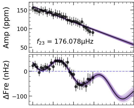
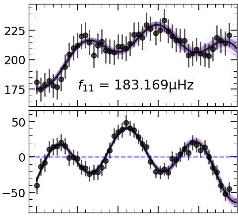
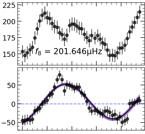
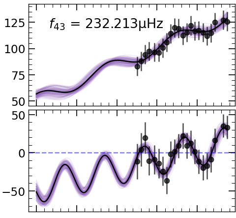
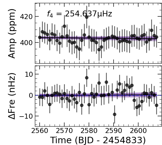
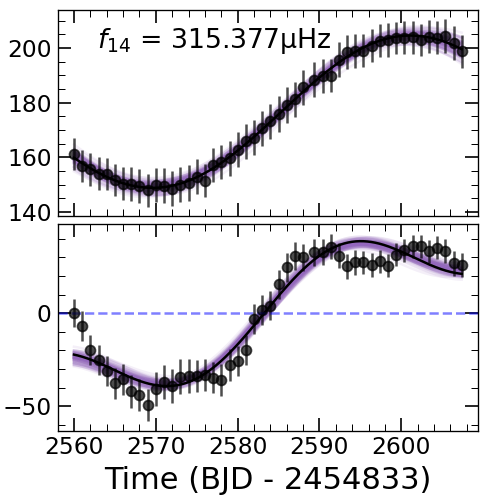
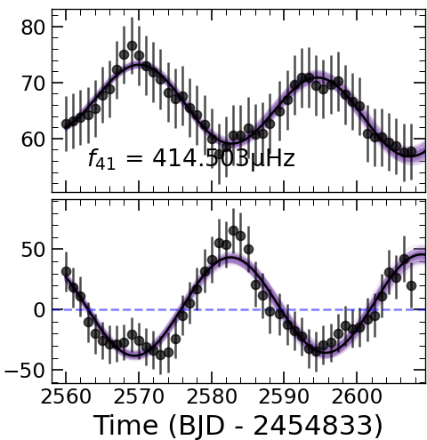
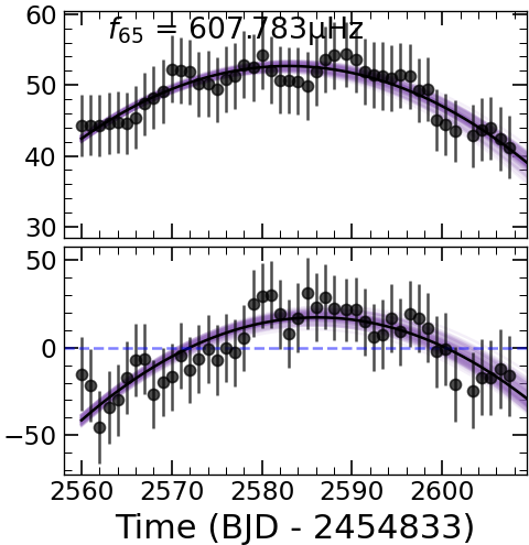
Figure 4: Gallery of eight typical frequencies with AM/FM variations. Each module contains AM (top panel) and FM (bottom panel) occurring in one single frequency. The frequencies are shifted to their averages as represented by the horizontal lines in each bottom panel. The solid curves in purple and black represent the fitting results from the MCMC method and the optimal model, respectively.

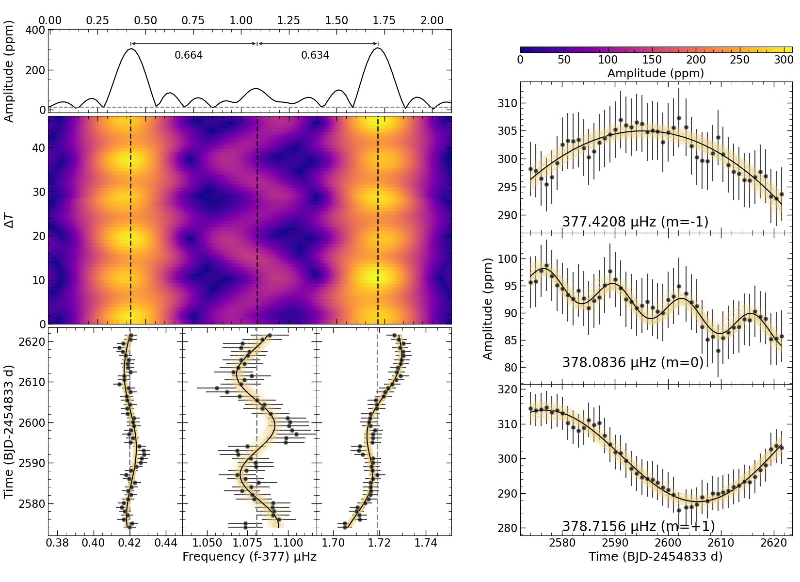
Figure 5: Frequency and amplitude modulation in the $g-$mode triplet near 377 $\mu$Hz. Top-left: Fine profile of the triplet in LSP, with near-symmetric frequency spacing. The dashed horizontal line represents the 5.2 $\sigma$ detection threshold. Middle-left: Sliding LSP giving a 3D view of the dynamics of the concerning triplet in general. Bottom-left: Expanded view of FM around the average frequency (vertical lines, also in the middle-left panel) of each component. Right: Measured amplitudes of the three components as a function of time obtained from each piece of light curves. The solid curves are the optimal fitting models of the AM and FM patterns, covering with MCMC uncertainties (see text for details).

Figure 5 displays the AMs and FMs for the three components that form the g-mode triplet near $377\,\mu$Hz. A close view of the profile of the triplet shows that the three components are not strictly systematically spaced in frequency. We measured a significant frequency mismatch of $\Delta f\sim 0.031\,\mu$Hz that is one order higher than the frequency uncertainty. The middle-left panel illustrates the dynamic patterns of frequency and amplitude over time through the sLSP diagram in a general way. A clear FM has been observed in the central component. Thus, we provide an expanded view centered on the average frequency of each component in the bottom-left panels, while their corresponding amplitude behaviors are presented in the right panels. With the current measuring precision in amplitude and frequency, we disclose the various modulating patterns in AMs and FMs of these three components. The optimal fitting and the associated MCMC curves suggest that the AMs and FMs follow simple patterns. During the $\sim 80$ day observations, the central component is found to exhibit modulation periods of $\sim 27$ days and 13 days for FM and AM, respectively, whereas the AM values show a slightly decreasing trend. Both the two side components exhibit FM with a similar period of $\sim 30$ d and vary in a small scale of a few nano Hz. We have observed some clear (anti-) correlation between the three resonant components. For instance, the two side components evolve somewhat in anti-phase both in amplitude and frequency with a similar timescale.

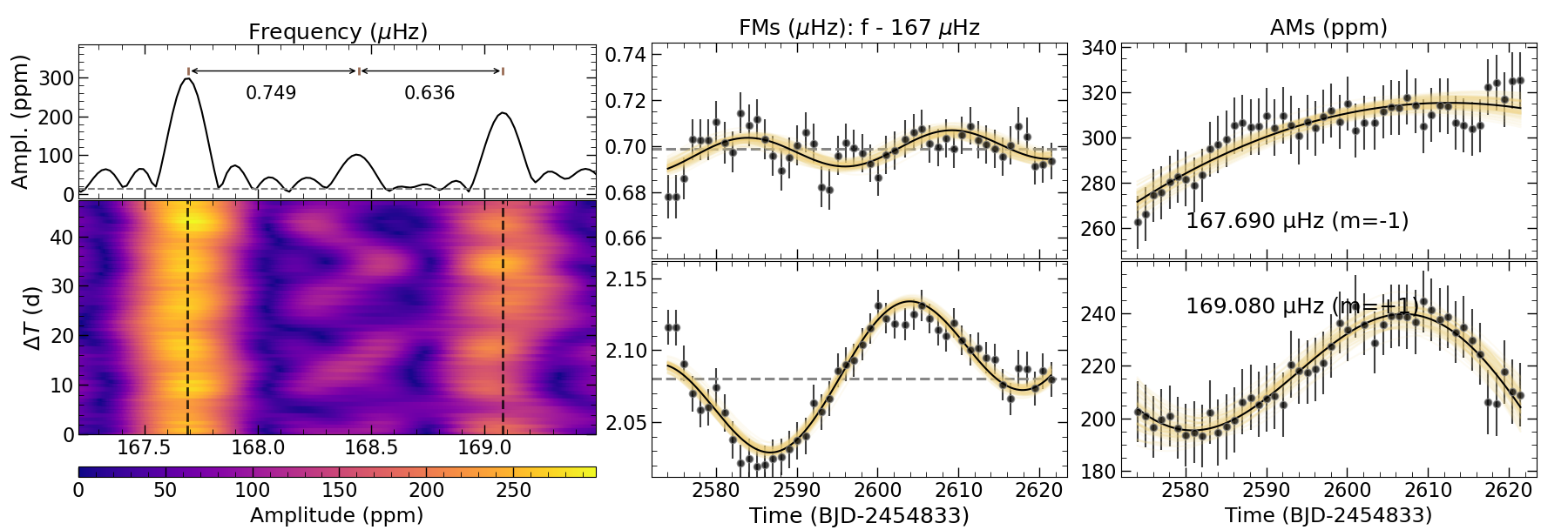
Figure 6: Similar to Fig. 5 but for the g-mode triplet near 167 $\mu$Hz, in a different layout of the sub-panels. Note: the AM and FM of the central component are not presented, as these measurements are limited by its low amplitude and large scale of the FM.

Figure 6 shows the behavior of AMs and FMs occurring in the two side components forming the triplet near 167 $\mu$Hz. From the LSP, a very large asymmetry is found in the frequency spacing of the three components, with a frequency mismatch of 0.105 $\mu$Hz. This could be related to the large FM of the central component (with a zigzag pattern), as revealed from the sliding LSP. However, it failed to explore piece-wise measurement of frequency for the central component due to its low amplitude. The retrograde component exhibits relatively stable frequency and amplitude from the sLPS. With piece-wise measurement, FM varies in a scale of a few nano Hz and AM exhibits a slightly increasing pattern from $\sim 270$ to 320 ppm. We note that the frequency uncertainty is comparable to the FM scale. The prograde component shows periodic patterns of FM and AM as indicated by the fitting models. The period of FM is comparable in both side components, $\sim 17$ days, if we ignore the slight linear trends.

3.2 Other AFMs

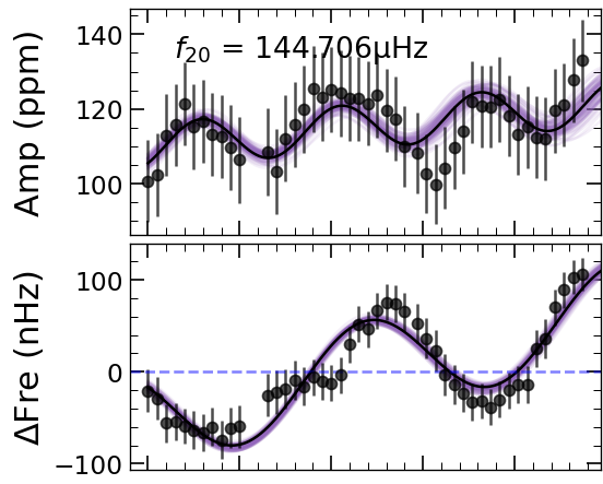
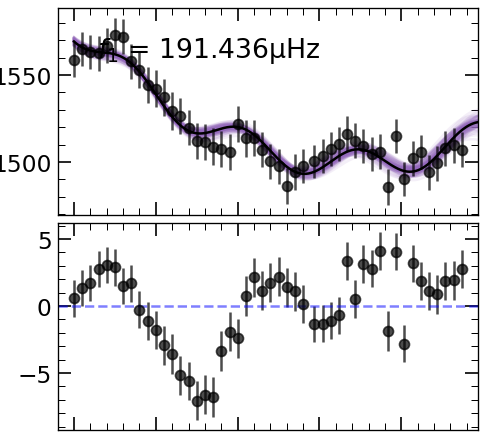
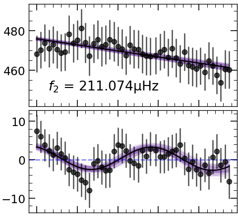
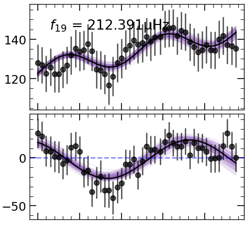
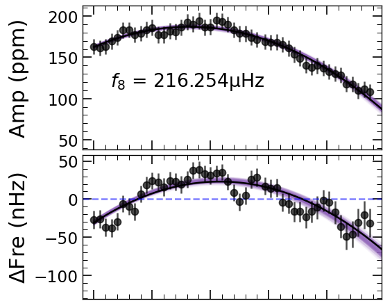
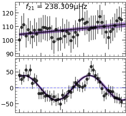
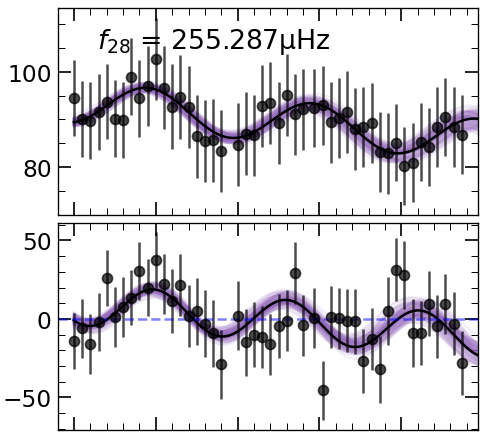
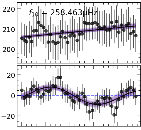
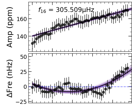
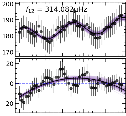
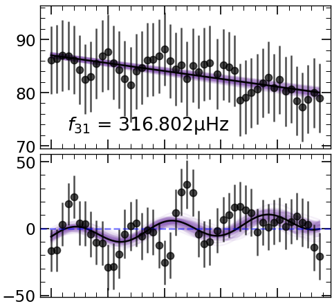
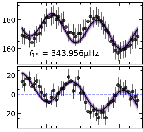
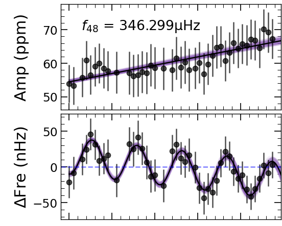
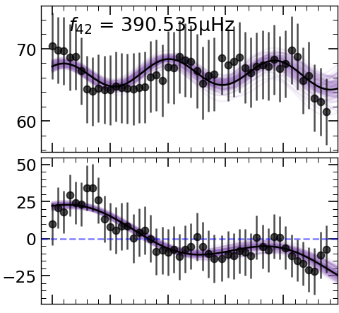
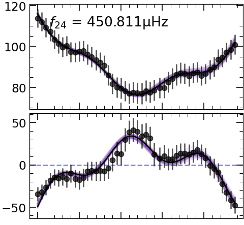
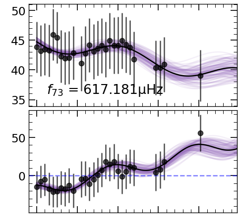
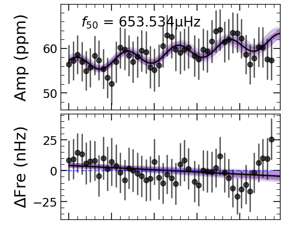
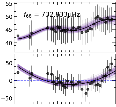
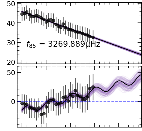
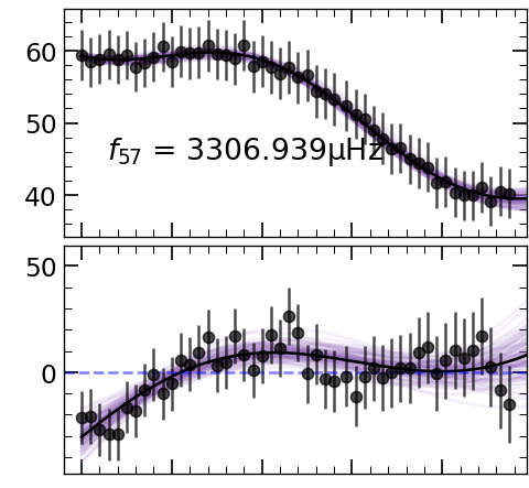
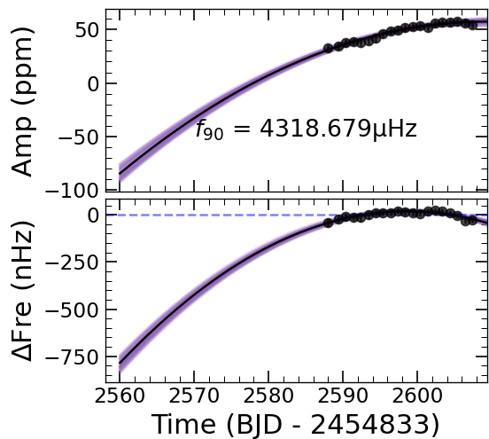
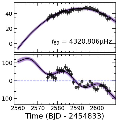
Figure 16: Gallery of 35 typical frequencies with AM/FM variations. Each module refers to the AM (top panel) and FM (bottom panel) variations of one single frequency. The frequencies are shifted to the average values as represented by the dashed horizontal lines, which are indicated in the bottom panel. The solid curves in purple and black represent the fitting results from the MCMC method and the optimal fitting, respectively.

Apart from the above AMs and FMs, the others are presented in Fig. 4 and Fig. 16. Overall, these modulations reveal rich and various patterns in PG 0101+039. Most of the observed modulations exhibit quasi-sinusoidal patterns with additional linear or parabolic fittings, namely, by fitting with $G_{4}$ or $G_{5}$. For instance, the AM and FM of $f_{24}\sim 450.8\leavevmode\nobreak\ \mu$Hz have evolved in anti-phase and exhibit a sinusoidal plus a parabolic pattern of $G_{5}$. Its amplitude decreases from $\sim 115$ ppm to the local minimum of $\sim 75$ ppm and rises afterward; correspondingly, the frequency varies from -50 nHz up to +50 nHz and returns back to -50 nHz relative to its average. Both the AM and FM of $f_{15}\sim 344.0\leavevmode\nobreak\ \mu$Hz exhibit a sinusoidal pattern with an additional linear fitting. There are a few frequencies that merely demonstrate somewhat sinusoidal patterns such as the FM of $f_{21}\sim 238.3\leavevmode\nobreak\ \mu$Hz and the AM of $f_{38}\sim 707.8\leavevmode\nobreak\ \mu$Hz. Some completely exhibit simple parabolic patterns, for instance, $f_{18}\sim 216.3\leavevmode\nobreak\ \mu$Hz whose AM and FM change in a scale of 100 ppm and 100 nano Hz, respectively. Several frequencies can be characterized by simple linear fitting of a decreasing or increasing amplitude and frequency. For instance, the frequency of $f_{59}\sim 571.5\leavevmode\nobreak\ \mu$Hz decreases nearly 70 nHz over an interval of $\sim 50$ days. We note that several modes exhibit visible amplitudes just over a fraction of the period during the observation such as $f_{90}\sim 4318.7\leavevmode\nobreak\ \mu$Hz and $f_{89}\sim 4320.7\leavevmode\nobreak\ \mu$Hz and there are also several modes whose amplitudes decrease down to detect threshold and vanish in the noise; for instance, $f_{85}\sim 3269.9\leavevmode\nobreak\ \mu$Hz.

There are only a few stable AMs and FMs, characterized for example, by a frequency and amplitude of $f_{4}\sim 254.6\leavevmode\nobreak\ \mu$Hz, or amplitudes of $f_{21}\sim 238.3\leavevmode\nobreak\ \mu$Hz and $f_{10}\sim 258.5\leavevmode\nobreak\ \mu$Hz modulating around 10 ppm. The majority of our discovered FMs are characterized within the range of $20-100$ nHz. One exceptional case is that $f_{20}\sim 144.7\leavevmode\nobreak\ \mu$Hz exhibits a large FM up to 200 nHz. We find a general correlation that the AMs and FMs are proportional to each other, that is: a mode that modulates on a large scale both in amplitude and frequency. Most of the concerning frequencies are on a modulating timescale of $\sim 30$ days and can be well resolved by the light curves. Interestingly, we observe several AMs with a relatively short period on a timescale down to $\sim 10$ days, for instance: AMs of $f_{5}\sim 378.1\leavevmode\nobreak\ \mu$Hz, $f_{36}\sim 574.0\leavevmode\nobreak\ \mu$Hz, and $f_{50}\sim 653.5\leavevmode\nobreak\ \mu$Hz. However, these quick patterns of AMs are very shallow (i.e., on the order of a few ppm, comparable to the amplitude uncertainties).

A notable feature of the (anti-) correlation is found between AM and FM among several frequencies. As listed in Table 2, the strongest correlation is found for $f_{14}\sim 315.4\leavevmode\nobreak\ \mu$Hz with a value up to 0.95. The strong anti-correlations are derived for the frequencies of $f_{41}\sim 414.5\leavevmode\nobreak\ \mu$Hz, $f_{24}\sim 450.8\leavevmode\nobreak\ \mu$Hz, and $f_{85}\sim 3269.9\leavevmode\nobreak\ \mu$Hz, with values of -0.82, -0.88, and -0.79, respectively. Several other frequencies also show strong correlation of $|\rho_{\mathrm{am,fm}}|>0.7$, for instance, $f_{23}\sim 176.1\leavevmode\nobreak\ \mu$Hz, $f_{18}\sim 216.3\leavevmode\nobreak\ \mu$Hz, $f_{12}\sim 314.1\leavevmode\nobreak\ \mu$Hz, and $f_{65}\sim 607.8\leavevmode\nobreak\ \mu$Hz. Additionally, we find that the FM of $f_{1}\sim 191.4\leavevmode\nobreak\ \mu$Hz and the AM of $f_{13}\sim 201.6\leavevmode\nobreak\ \mu$Hz exhibit quasi-regular behavior. However, their patterns cannot be fitted by our simple $G_{k}$ functions. As a result, we reserve not to perform fitting or apply EMCEE on these relatively complicated AMs and FMs. Finally, we note that most of these AMs and FMs change in scales in a similar order like a few tens of ppm and micro Hz, respectively.

4 Discussion

In the previous sections, we describe our analysis of the K2 photometry of PG 0101+039 and our detections of rich pulsation signals for the first time, which offer an opportunity to investigate the properties of those pulsation modes from linear to nonlinear way. With splitting frequencies, we derived a rotation period of $\sim 8.81\pm 0.06$ and $8.60\pm 0.16$ days by the g-modes and p-modes, respectively, implying a marginally differential rotation with a probability of $\sim 60\%$. Thus, this suggests that PG 0101+039 is now clearly an unsynchronized system with the orbital period of $0.570$ days (Geier et al., 2008). In this section, we discuss the rotational and orbital properties, as well as the dynamics of amplitude and frequency of oscillation modes.

4.1 Binary information

As reported in the literature (Moran et al., 1999; Randall et al., 2005; Geier et al., 2008), PG 0101+039 has been considered a highly probable synchronized system due to its close orbit of about half a day, requiring the tidal force to be strong enough for the synchronization process to begin. Recently, Schaffenroth et al. (2023a) analyzed K2 data collected on PG 0101+039 and concluded that the orbital light variation is dominated by the beaming effect and accompanied by tiny ellipsoidal deformation. These authors derived a very high orbital inclination that is close to $89.4^{\circ}\pm 0.06^{\circ}$, which, in turn, suggests that the companion is probably a helium-core white dwarf with a mass of $0.34\pm 0.04\,M_{\odot}$. In addition, they derived the rotation period of $0.85\pm 0.09$ days for PG 0101+039 based on $v\sin i$ from spectroscopy, which is slightly slower than its orbital period. This is the first claim that PG 0101+039 should be in a non-synchronized system.

From our thorough analysis of the pulsation signals, we firmly derived a rotation period of $\sim 9$ days based on frequency splitting. This rotation rate is about $\times 10$ slower than the preliminary result by Schaffenroth et al. (2023a), which means that the rotational velocity measured by Geier et al. (2008) is overestimated heavily. Interestingly, we find that the rotation period derived from p-modes, $8.60\pm 0.16$ days, is slightly faster than that coming from g-modes, namely, $8.81\pm 0.06$ days, although this differential is marginally and comes with a probability of $\sim 60\%$. In general, p-modes propagate outer parts than g-modes, which means that PG 0101+039 has a radial differential rotation with a relatively faster envelope. From the Kepler/K2 photometry, two sdB pulsators have been reported to have radial differential rotations via p- and g-multiplets, KIC 3527751 (Foster et al., 2015) and EPIC 220422705 (Ma et al., 2022), even the former were challenged by Zong et al. (2018). We stress that PG 0101+039 is among them with the fastest rotation and orbit. If we consider the tidal effect from the companion, it would be a natural case that the envelope rotates faster than the inner part. The tidal force introduces internal gravity modes, which are located between the radiative envelope and the convective core, then it transports angular momentum to the out layer, leading to the envelope becoming first synchronized and then gradually proceeding to the inner part (Goldreich & Nicholson, 1989). The radial differential sdB pulsators are on the way to being synchronized and could be used for the stellar chronology of binary systems. Therefore, we paid attention to the binary information of PG 0101+039 from both photometry and spectroscopy.

For PG 0101+039, we collected 50 high-quality spectra with S/N ¿ 10 from the LAMOST DR8. They were observed under the LK-MRS projects during 2018-2019 (see details in Zong et al., 2020) and exhibit a medium resolution of $R\sim 7500$, covering the wavelength of 495-535 nm and 630-680 nm in two bands (Yan et al., 2022). As we only analyzed the binary signals, we only considered the radial velocity (RV) of PG 0101+039 derived from these spectra. We note that all spectra are found to be single-line dominated as a consequence of the high contrast of light fraction between the sdB and the companion. Among several pipelines to measure the RVs of LAMOST spectra, we chose the RVs from Zhang et al. (2021), who adopted the cross-correlation function method. In addition, they have proposed a robust method for a self-consistent determination that aims to correct the systematic zero-point RV offsets, combined with the RVs from the Gaia DR2 (Katz et al., 2019). We list the information of those RVs in Table F, with the attributes of observation time, RVs, and associated errors, as well as the S/N values. We first adopted the method of phase dispersion minimization (PDM) to derive the period of the RV curves. Then we used the Keplerian orbit to fit the radial velocities around the PDM period $\sim 0.5699$ d (see Fig. 7, a). The fitting result of the orbital solution is obtained through the EMCEE code (see, Foreman-Mackey et al., 2013, for a review) and their parameters are provided in Table 3. We then derived the mass limit, $M_{2}\geq 0.36$ M_⊙, for the companion based on the mass function and assumed the sdB star with a canonical mass of $M_{1}=0.47$ M_⊙. Our results are overall consistent with the orbital parameters derived from previous literature (Moran et al., 1999; Geier et al., 2008; Schaffenroth et al., 2023a), as compared in Table 3

Table 3: Orbital parameters derived by the EMCEE code v.s. the results from the literature.

$P$	$\gamma$	$K$	$\omega$	$e$	$a$	$i$	$M_{\mathrm{2,min}}$	Reference
(d)	(km s-1)	(km s-1)	(∘)		($\mathrm{R_{\odot}}$)	(∘)	($\mathrm{M_{\odot}}$)
$0.5699079\pm 0.0000068$	$8.47\pm 0.34$	$104.29\pm 0.47$	–	–	–	–	$0.37\pm 0.02$	[1]
$0.569899\pm 0.000001$	$7.3\pm 0.2$	$104.5\pm 0.3$	–	–	$3.1\pm 0.4$	$40\pm 6$	$0.45$	[2]
–	–	–	–	–	$2.53\pm 0.01$	$89.4\pm 0.6$	$0.33$	[3]
$0.5698990^{+0.0000003}_{-0.0000004}$	$6.9^{+\,0.2}_{-\,0.3}$	$105.0^{+\,0.2}_{-\,0.4}$	$82.4^{+\,3.8}_{-\,8.5}$	$0.032^{+\,0.002}_{-\,0.004}$	–	–	$0.36$	This work

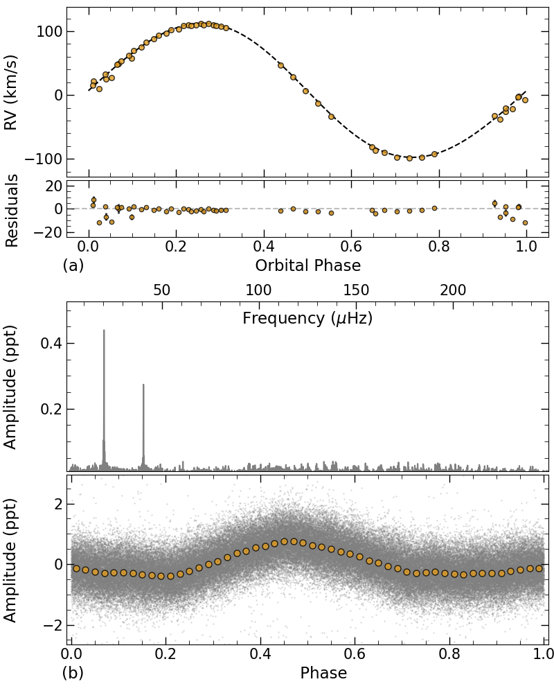
Figure 7: Orbital signals of radial velocity and photometry. (a) Phase-folded radial velocities with a Keplerian orbit fitting for the binary system and residuals. Uncertainties are included but are smaller than the symbols themselves for most measurements. (b) LSP of the orbital signals with the removal of oscillation signals (top panel) and the corresponding phase-folded light curve (bottom panel). Note: the K2 photometry is averaged into 50 measurements by their phase (filled cycles).

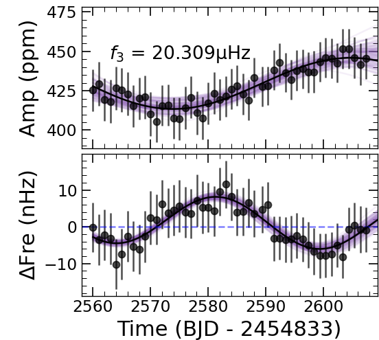
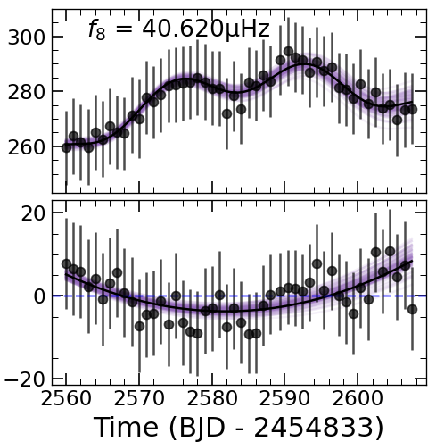
Figure 8: AMs and FMs of the orbital frequency and its harmonic overtone.

The LSP of the photometry clearly shows low-frequency signals that are attributed to the orbital brightness variations. Their frequencies are derived with $\sim 20.3107\pm 0.0015\leavevmode\nobreak\ \mu$Hz, or $0.569851\pm 0.000042$ d, for the primary peak (see Fig. 7, b). We note there is some phase difference between the photometry and RV curve, mainly introduced by the fact that these two curves were folded into phase by their own ephemeris and optimal periods with very slight differences. If we stick folding curves with the same period, the scatter will be a bit larger in one curve, which deserves some particular attention in the future. When we exploit the dynamics of those two orbital signals, we clearly find that both their frequency and amplitude show quasi-periodic modulations (Fig. 8). The modulating patterns are not exactly the same as the AMs and FMs observed for pulsation modes if we compare the fitting results in Table 2. More specifically, it is only the orbital signal $f_{3}$ exhibits sinusoidal patterns in both the AM and FM. This can be explained if the companion is indeed an active star presenting magnetic variability (e.g., spot modulation). Recently, Pan et al. (2020) and Wang et al. (2022) suggest that spot activity in late-type M dwarf can introduce amplitude and frequency modulations to the signals related to the orbit in the Fourier space. Therefore, PG 0101+039 could possibly contain an active companion of an M-dwarf star, different from the claiming of a helium white dwarf by Schaffenroth et al. (2023a). Moreover, from the summarized information of the sdB pulsator in binary system (Silvotti et al., 2022), there is no sdB+WD system that contains a sdB companion with $P_{\mathrm{rot}}<10$ days; for instance, EPIC 201206621, with $P_{\mathrm{orb}}\sim 0.54$ d and $P_{\mathrm{rot}}>45$ d (Reed et al., 2016) and EPIC 211696659, with $P_{\mathrm{orb}}\sim 3.2$ d and $P_{\mathrm{rot}}>28$ d (Reed et al., 2018), whereas a sdB+dM binary usually has a relatively faster rotating sdB pulsator with $P<10$ days such as EPIC 246023959 with $P_{\mathrm{orb}}\sim 0.31$ d and $P_{\mathrm{rot}}\sim 4.6$ d and EPIC 246387816 with $P_{\mathrm{orb}}\sim 0.80$ d and $P_{\mathrm{rot}}\sim 9.4$ d (Baran et al., 2019). To conclude, the type of the faint companion of PG 0101+039 is still not well determined. Further work to identify the type of companion based on combining photometry and spectroscopy is strongly encouraged. Finally, we note that this unsynchronized system can be used as an independent method to determine the age of the sdB binaries. Because the ratio of the differential rotation rate between the core and envelope can be calculated through the dynamical process of tidal synchronization(Nicholson, 1979; Goldreich & Nicholson, 1989). This can be further studied after obtaining more precise parameters for the primary and the secondary components.

4.2 Nonlinear modulation

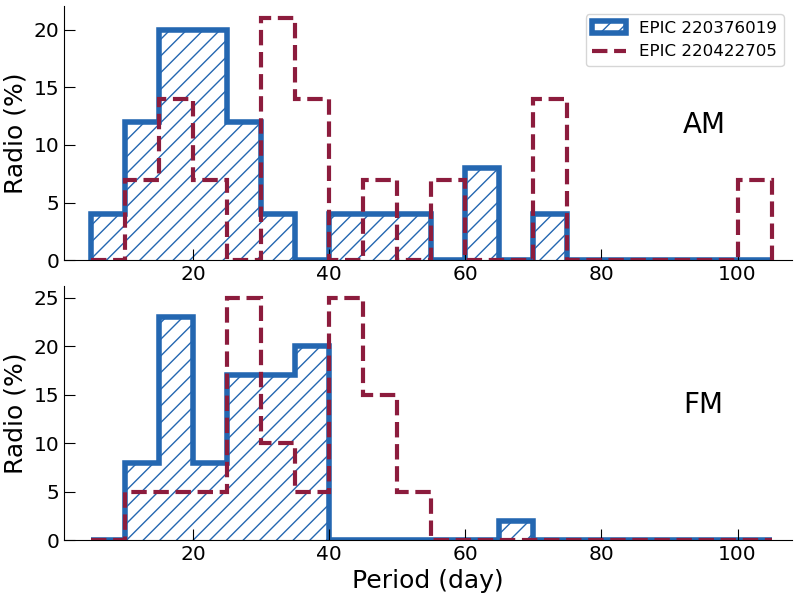
Figure 9: Period distributions of AMs and FMs that are characterized in EPIC 220396019 and EPIC 220422705.

In PG 0101+039, we have clearly detected amplitude and frequency variations in 44 frequencies, most of which are characterized by periodic modulation patterns, for instance, by the fitting of a $G_{4}$ function. Instead of the AMs and FMs in EPIC 220422705 (Ma et al., 2022), where the close frequencies can introduce the beating effect, the modulations in PG 0101+039 are mostly intrinsic as the rotational multiplets are well resolved. As first documented in Zong et al. (2016a), periodic AMs and FMs in sdB pulsator are related to nonlinear resonant mode coupling. In their following results, they found that the pulsation modes in sdB stars are commonly observed to exhibit AM and FM (Zong et al., 2018, 2021). However, the AMs and FMs measured from Kepler photometry exhibit a time resolution of a few tens of days and the modulating timescales are characterized from months to years. With K2 photometry, the time resolution of AMs and FMs is reduced to 1 d, which leads to discoveries of short timescale variations of $\sim 30$ d in EPIC 220422705 and PG 0101+039. Compared to the former, oscillation modes in PG 0101+039 generally have a shorter modulating timescale. Figure 9 shows the periods of AMs and FMs in those two sdB pulsators. For instance, the AMs in PG 0101+039 are found around a period of 20 d, but those of EPIC 220422705 are distributed in a wider range from 20 d to 70 d.

According to the nonlinear regime (see, e.g., Goupil et al., 1998), the modulating timescale could be roughly estimated to the inverse of the frequency mismatch between three resonant modes as

$$P_{\mathrm{m}}\sim 1/\delta f,$$ (3)

where the $\delta f=i\cdot f_{1}+j\cdot f_{2}-k\cdot f_{3}$. We typically consider $[i,j,k]=[1,1,1]$ and $[i,j,k]=[1,1,2]$ for direct resonance and rotational triplet resonance, respectively. In the triplet case, $\delta f\propto\Omega^{2}/f$ indicates that a faster rotation introduces a larger frequency mismatch (Dziembowski & Goode, 1992). It would be natural to foresee a relatively rapid AM and FM in the faster rotating star compared to the slower one if we completely base on Eq. 3. As we mentioned before, the modulating periods derived for PG 0101+039 are somewhat shorter than those of EPIC 220422705. The rotation periods of PG 0101+039 and EPIC 220422705 are $\sim$ 9 d and 35 d, respectively, whereas the latter has a typical rotation rate of sdB pulsators, ranging from a few days to several months, for instance, $P_{\mathrm{rot}}$ (KIC 5807616) $\sim$ 39 d (Charpinet et al., 2011a) and $P_{\mathrm{rot}}$ (EPIC 212707862) $\sim$ 80 d (Bachulski et al., 2016). The theoretical prediction can be well consistent with the observation if one imagines that most modes are in triplet resonance. Therefore the ratios of period derived for AMs and FMs in those two stars are clearly distinct. However, we address the point that it is very hard to calculate the modulating timescales precisely for the observed AMs and FMs from the theoretical aspect at present. This is because we have to first construct linear seismic models to obtain linear eigenvalues for the resonant modes, which are the base vectors for further calculation of the complicated nonlinear coefficients that are involved in nonlinear amplitude equations (Dziembowski, 1982).

Another important result, related to nonlinear resonance, is that we have observed many pulsation modes exhibiting high (anti-) correlation between AMs and FMs. This finding is also recently disclosed in other sdB pulsators, for instance, KIC 3527751 (Zong et al., 2018) and EPIC 220422705 (Ma et al., 2022). For a three-mode interaction, the nonlinear amplitude equations (AEs) can be simplified as follows:

$$\mathbf{\dot{A}}_{i}=\mathbf{Q}(\mathbf{A}_{i},\mathbf{A}_{j},\mathbf{A}_{k}),$$ (4)

where $i,j,k=1,2,\leavevmode\nobreak\ \mathrm{or}\leavevmode\nobreak\ 3,$ with $i\neq j\neq k$, and the $\mathbf{Q}$ is a function involving nonlinear complicated coupling coefficients. We can see details of nonlinear AEs in, for instance, Moskalik (1985). The complex amplitude $\mathbf{A}_{i}$ can be separated into the real part, $A_{i}$, and the imaginary part, $\phi_{i}$. The time deviation, or temporal variation, of the real part forecasts AM, whereas the imaginary part is for FM. Numerical explorations of nonlinear AEs explicitly show several cases of anti-correlation between AMs and FMs (Moskalik, 1985). As the nonlinear AEs are governed by their amplitudes, it is natural to foresee that FMs follow the behavior of AMs. Our findings, therefore, are further consistent with the prediction of nonlinear AEs, which can also be used for the upcoming nonlinear calculations. In addition, the observation of non-modulating modes could be non-resonant modes with very slight nonlinear couplings or nonlinear locking modes with too strong couplings. Those modes are suitable for exoplanet detection or monitoring secular evolutionary period changing rates via pulsation-timing technique.

In PG 0101+039, we reported an additional feature that is different from the modulating patterns in previous studies. Within the same multiplet, one of them may exhibit a much shorter timescale compared to others, for instance, the AM of the frequency near $574\leavevmode\nobreak\ \mu$Hz (Figure 14). To verify the intrinsic of this shallow and rapid AM, we changed the window of the sLSP in various widths and we never saw any significant changes in AM. This suggests that the observed modulations might be more complicated than the simple explorations of nonlinear resonance where only the weak interaction of one kind of resonant mode was considered to avoid complicated calculations of nonlinear AEs (see, e.g., Goupil & Buchler, 1994; Buchler et al., 1995). As previously reported in Zong et al. (2016a), it has been suggested that the observed AMs and FMs could play a role in different kinds of resonance simultaneously, as a consequence that solely the rotation resonance might not be enough to explain their specific AMs and FMs. Therefore, these current discoveries strongly indicate that the nonlinear calculation of AEs with different types of resonance has to be considered in the future, in order to mimic the complicated AMs and FMs from observations. However, in the multiplet component near $574\leavevmode\nobreak\ \mu$Hz, we did not resolve any linear combinations that could be linked to direct resonance at present. There might be several combining modes in potential, but their amplitude is far below the current noise.

Finally, we notice that amplitude and frequency modulating in a short timescale is important to the development of nonlinear stellar theory in the future. Compared to the Kepler discoveries, it will extend the investigating sample of nonlinear resonance to a much larger volume for the first time. As complementary, various modulating behaviors and timescales are useful constraints to various nonlinear quantities involved in AEs.

5 Conclusion

PG 0101+039 has been continuously observed by K2 in Campaign 8 over a period of $\sim 79$ days. Its photometry was extracted from the TPF file with a series of pixel sizes. The optimal aperture is estimated to be 12 for following Fourier transformation by evaluating the S/N of the primary frequency (Fig. 1). Both the light curves and the Lomb-Scargle periodogram reveal that PG 0101+039 is a $g$-mode-dominated hybrid pulsating sdB star. By setting the threshold of $\mathrm{S/N}=5.2$, we detected 137 independent frequencies (including ten frequencies whose S/N $<5.2$ ), two orbital frequencies and 51 linear combinations. The former includes 20 rotational multiplets with 70 identified components (Fig. 3). Those frequency splittings give a rotational period of $8.81\pm 0.06$ d and $8.60\pm 0.16$ d for the internal part and outer layer, as g-modes penetrate deeper than p-modes, implying a marginally radial differential rotation with a probability of $\sim 60\%$. This explanation could be supported that tidal force can initially accelerate the envelope by introducing internal gravity wave (Goldreich & Nicholson, 1989). We exploit the binary information combined with spectroscopy and photometry, coming up with a solution similar to previous results (Moran et al., 1999; Geier et al., 2008). It suggests that this binary system is still on the way to synchronization with an orbital period of $0.57$ d and a rotational period of $\sim 8.8$ d. However, we stress that the conclusion of differential rotation is based on relatively weak evidence if one fully considers the uncertainties in the period of rotation. We then derive the period spacing of $\sim$252 s and 144 s for dipole and quadrupole modes, respectively. Subsequently, we identified 28 frequencies in the dipole mode sequence, 28 quadrupole modes, and another 3 in both sequences.

Before we proceeded to characterize amplitude and frequency modulations, we performed a series of testing to prove that modulating pattern is independent of the size of the stamp, thanks to the relative isolate position of PG 0101+039. At this stage, we can exploit the amplitude and frequency modulations for 44 significant pulsations. The majority of those pulsations exhibit clear modulating behavior in various patterns, which can then be characterized by five types of simple functions. The fitting uncertainties were derived with the MCMC technique. We find that the majority of these modulating patterns can be presented with a periodic fitting and these modulating periods are on a timescale of months, or precisely, in the range between $\sim 10-70$ days. There are four frequencies modulating in a much more rapid period, slightly less than 10 days. In general, we observe a relatively short timescale of AMs and FMs in PG 0101+039. Interestingly, many frequencies show a clear high (anti-) correlation between their amplitude and frequency. Moreover, we find that two low-frequency signals, related to the orbit, present amplitude and frequency variations as well.

To interpret the discovered AMs and FMs of oscillation modes in PG 0101+039, a natural consequence could be produced by nonlinear resonant couplings which predicts various variations in amplitude and frequency (see, e.g., Goupil et al., 1998). In some particularly resonant conditions, the nonlinear interacting modes undergo periodic variations (Buchler et al., 1995), as we indeed observe many modes that exhibit periodic modulating patterns; these, in particular, serve as evidence of several multiple components. As the modulating period, $P_{\mathrm{m}}$, is proportional to the frequency mismatch or higher order effect from rotation, in general, $P_{\mathrm{m}}$ has somewhat smaller values in PG 0101+039 than EPIC 220422705 as the former has a relatively faster rotation comparing to the latter. The (anti-) correlation between AMs and FMs further supports our explanation since the patterns of FMs are governed by that of AMs when one tries to solve the nonlinear amplitude equations in a numerical way (Moskalik, 1985). However, at the current stage, we are still waiting for the seismic model to calculate the linear eigenvalues for the nonlinear coupling modes, upon which the nonlinear coupling coefficients are built. Moreover, the AMs and FMs exhibit somewhat more complicated patterns than the prediction from nonlinear AEs, in which the assumption only considers three interacting modes within one kind of resonance. These modulating patterns probably offer observational constraints to future calculations of nonlinear amplitude equations. This shorter timescale modulation should be explored in other sdB stars that had been observed by K2 and TESS. We finally note that this finding could jeopardize the exoplanet detection via the time-pulsation method (Silvotti et al., 2007, 2018). Because the phase modulation can hardly be well derived if we do not have information a priori on the frequency modulations.

Appendix A The optimal stamp for the light curve

To find the optimal stamp for PG0101 039, we considered a series of stamps with different pixel sizes from the TPFs. The stamp was initially covered by ten pixels with the highest values of flux, thanks to PG 0101+039 being free of flux contamination. Then the stamp was expanded outward to nearby pixels in sequence according to their values of flux down to around 30, a level similar to a few times of background. In our case, the stamp is composed of 38 pixels that completely cover the target, as shown in Fig 10 (b) by the pixels in grey shadow and surrounded by the dashed lines. For each stamp enlargement, we extracted the light curves for PG 0101+039 and performed some preliminary processes on them, including detrending and outlier clipping. A few outliers were clipped off from the overall flattened light curves by filtering with a local 3.5$\sigma$ threshold. Then the light curves were normalized and performed with Fourier transformation for quality comparison. The signal-to-noise ratio (S/N) of the signal with the highest amplitude ($\sim 191.5\,\mu$Hz) was denoted to represent the quality of the light curves. The recorded S/N for each light curve is shown in Fig 1 (a), with values from 222 to 273. The highest S/Ns are found around pixel sizes of around 12 to 16. We thus took the optimal stamp with 12 central pixels and the corresponding light curves were used according to our following analysis, a similar strategy to Duan et al. (2021).

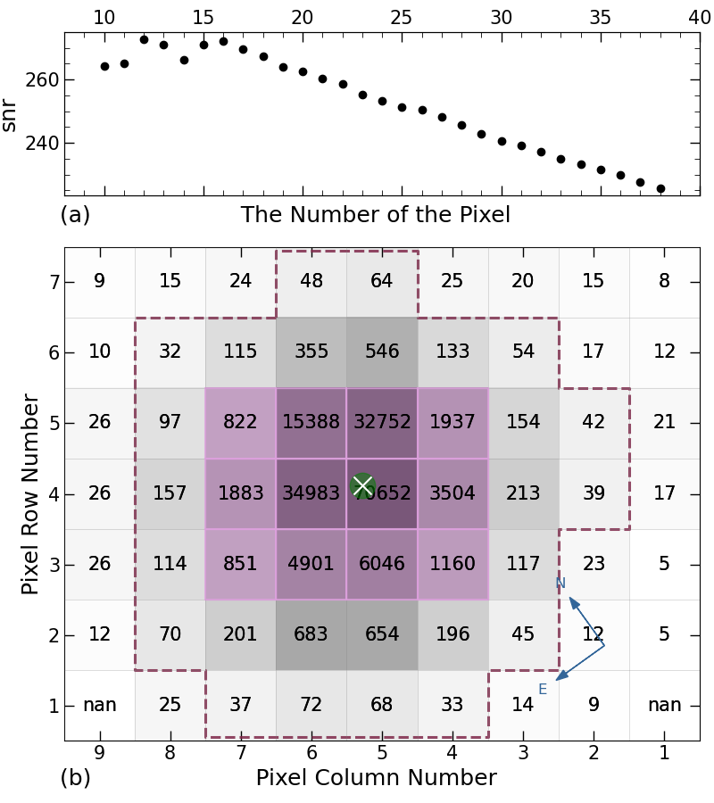
Figure 10: Aperture selection of TPFs. Fig (a) shows how the SNR of the frequency with the highest amplitude varies from the number of pixels. (b) The TPFs with the median value of PG 0101+039. The size of the green dot represents the relative brightness of the star, and the white ’$\times$’ is the location of our target star. The plum boxes are the pixels used for extraction.

Appendix B All frequencies detected in PG 0101+039

Table 4: All frequencies we detected in PG 0101+039 by order of increasing frequency.

ID	Frequency	$\sigma$f	Period	$\sigma$P	Amplitude	$\sigma$A	S/N	$\ell$	$m$	Mode	Comments
	($\mu$Hz)	($\mu$Hz)	(s)	(s)	(ppm)	(ppm)
$f_{74}$	84.1622	0.0149	11881.8220	2.1086	39.11	7.21	5.4	$1^{*}$	$-1^{*}$	$g$	…
$f_{55}$	109.5365	0.0116	9129.3736	0.9698	52.20	7.49	7.0			$g$	…
$f_{62}$	111.6446	0.0128	8956.9917	1.0249	48.05	7.57	6.3			$g$	…
$f_{54}$	112.4960	0.0117	8889.2042	0.9258	52.62	7.60	6.9	$2^{*}$	$-2^{*}$	$g$	…
$f_{63}$	114.3497	0.0128	8745.1024	0.9756	47.73	7.51	6.3	$2^{*}$	$-2^{*}$	$g$	…
$f_{53}$	119.0652	0.0116	8398.7592	0.8153	53.25	7.59	7.0	$1^{*}$	$-1^{*}$	$g$	…
$f_{49}$	121.3440	0.0108	8241.0347	0.7321	57.56	7.65	7.5	$1^{*}$	$1^{*}$	$g$	…
$f_{26}$	124.8665	0.0070	8008.5516	0.4500	89.49	7.74	11.6			$g$	…
$f_{61}$	138.5549	0.0134	7217.3580	0.6996	48.55	8.05	6.0	$2^{*}$	$-2^{*}$	$g$	…
$f_{44}$	144.0292	0.0104	6943.0373	0.5018	62.52	8.03	7.8	1	0	$g$	…
$f_{20}$	144.7187	0.0055	6909.9594	0.2630	117.88	8.01	14.7	1	1	$g$	AFM
$f_{30}$	155.3015	0.0076	6439.0879	0.3169	84.75	7.99	10.6	1	0	$g$	…
$f_{37}$	155.9591	0.0090	6411.9392	0.3690	72.00	7.97	9.0	1	1	$g$	…
$f_{56}$	157.1873	0.0127	6361.8370	0.5152	50.79	7.98	6.4			$g$	…
$f_{32}$	163.1337	0.0082	6129.9395	0.3063	79.04	7.95	9.9	$2^{*}$	$-1^{*}$	$g$	…
$f_{7}$	167.6954	0.0021	5963.1940	0.0739	302.10	7.74	39.0	1	-1	$g$	AFM
$f_{27}$	168.4449	0.0070	5936.6595	0.2469	89.20	7.71	11.6	1	0	$g$	…
$f_{9}$	169.0794	0.0030	5914.3814	0.1045	209.27	7.71	27.1	1	1	$g$	AFM
$f_{23}$	176.0551	0.0063	5680.0400	0.2049	99.85	7.82	12.8	$1^{*}|2^{*}$	$0^{*}|-2^{*}$	$g$	AFM
$f_{34}$	180.3555	0.0082	5544.6053	0.2524	75.95	7.69	9.9	$2^{*}$	$-2^{*}$	$g$	…
$f_{35}$	182.5338	0.0082	5478.4369	0.2454	75.49	7.62	9.9	1	-1	$g$	…
$f_{11}$	183.1629	0.0031	5459.6210	0.0916	200.91	7.61	26.4	1	0	$g$	AFM
$f_{58}$	183.8808	0.0122	5438.3060	0.3616	50.05	7.55	6.6	1	1	$g$	…
$f_{42}$	185.6676	0.0092	5385.9685	0.2664	66.64	7.55	8.8	$2^{*}$	$-2^{*}$	$g$	…
$f_{1}$	191.4365	0.0004	5223.6643	0.0108	1532.74	7.52	203.9	$1^{*}|2^{*}$	$0^{*}|2^{*}$	$g$	AFM
$f_{66}$	200.5844	0.0130	4985.4327	0.3234	45.26	7.26	6.2	2	-1	$g$	…
$f_{13}$	201.6434	0.0032	4959.2499	0.0785	181.95	7.16	25.4	2	0	$g$	AFM
$f_{40}$	202.5375	0.0086	4937.3562	0.2105	67.37	7.18	9.4	2	1?	$g$	…
$f_{2}$	211.0751	0.0012	4737.6492	0.0264	466.68	6.77	69.0	$2^{*}$	$0^{*}$	$g$	AFM
$f_{19}$	212.3919	0.0041	4708.2776	0.0918	130.76	6.68	19.6	$1^{*}$	$0^{*}$	$g$	AFM
$f_{18}$	216.2481	0.0036	4624.3181	0.0761	146.22	6.42	22.8			$g$	AFM
$f_{70}$	218.8927	0.0124	4568.4489	0.2582	41.96	6.40	6.5	$2^{*}$	$-1^{*}$	$g$	…
$f_{81}$	225.4701	0.0139	4435.1780	0.2736	34.96	6.00	5.8	$2^{*}$	$-1^{*}$	$g$	…
$f_{43}$	231.0496	0.0074	4328.0757	0.1381	64.10	5.83	11.0	2	-1	$g$	…
$f_{46}$	232.1609	0.0076	4307.3583	0.1407	61.37	5.74	10.7	$2^{*}$	$0^{*}$	$g$	AFM
$f_{64}$	234.3496	0.0096	4267.1295	0.1757	47.33	5.63	8.4	2	2	$g$	…
$f_{21}$	238.2989	0.0040	4196.4107	0.0698	110.22	5.39	20.4	$1^{*}$	$0^{*}$	$g$	AFM
$f_{45}$	239.5982	0.0070	4173.6544	0.1211	62.25	5.34	11.7	$2^{*}$	$1^{*}$	$g$	…
$f_{51}$	250.3381	0.0072	3994.5983	0.1150	55.15	4.90	11.2			$g$	…
$f_{4}$	254.6364	0.0009	3927.1685	0.0146	404.06	4.71	85.8	1	0	$g$	S
$f_{28}$	255.2867	0.0043	3917.1639	0.0665	88.47	4.73	18.7	1	1	$g$	AFM
$f_{10}$	258.4635	0.0018	3869.0180	0.0273	207.41	4.67	44.4			$g$	AFM
$f_{97}$	260.7369	0.0134	3835.2831	0.1977	27.72	4.60	6.0			$g$	…
$f_{114}$	281.9538	0.0150	3546.6802	0.1887	22.08	4.09	5.4	$2^{*}$	$-2^{*}$	$g$	…
$f_{22}$	291.0652	0.0031	3435.6564	0.0362	101.26	3.84	26.4	1	-1	$g$	AFM
$f_{17}$	291.7374	0.0021	3427.7404	0.0244	149.76	3.83	39.1	1	0	$g$	AFM
$f_{47}$	293.5365	0.0052	3406.7318	0.0598	59.65	3.79	15.7	$2^{*}$	$-2^{*}$	$g$	…
$f_{16}$	305.5117	0.0019	3273.1966	0.0202	152.56	3.55	43.0	$2^{*}$	$-2^{*}$	$g$	AFM
$f_{12}$	314.0817	0.0015	3183.8846	0.0150	187.03	3.42	54.7	$1^{*}$	$0^{*}$	$g$	AFM
$f_{14}$	315.3790	0.0016	3170.7879	0.0159	174.72	3.41	51.3			$g$	AFM
$f_{31}$	316.7995	0.0034	3156.5707	0.0341	80.68	3.41	23.7			$g$	AFM
$f^{*}_{174}$	329.9880	0.0187	3030.4133	0.1716	14.22	3.28	4.3	2	-2	$g$	…
$f^{*}_{145}$	331.0714	0.0158	3020.4962	0.1442	16.80	3.28	5.1	2	-1	$g$	…
$f_{84}$	332.1861	0.0079	3010.3603	0.0711	33.87	3.28	10.3	$2^{*}$	$0^{*}$	$g$	…

Table 4: continued.

ID	Frequency	$\sigma$f	Period	$\sigma$P	Amplitude	$\sigma$A	S/N	$\ell$	$m$	Mode	Comments
	($\mu$Hz)	($\mu$Hz)	(s)	(s)	(ppm)	(ppm)
$f_{94}$	333.2654	0.0091	3000.6119	0.0822	29.11	3.28	8.9	2	1	$g$	…
$f_{103}$	334.3583	0.0107	2990.8035	0.0960	24.70	3.27	7.5	2	2	$g$	…
$f_{69}$	343.3255	0.0061	2912.6879	0.0515	42.30	3.17	13.3	1	-1	$g$	…
$f_{15}$	343.9567	0.0015	2907.3428	0.0128	169.36	3.15	53.7	1	0	$g$	AFM
$f_{78}$	350.7326	0.0066	2851.1747	0.0534	37.44	3.03	12.3	$2^{*}$	$-2^{*}$	$g$
$f_{06}$	377.4207	0.0008	2649.5631	0.0053	302.17	2.84	106.4	1	-1	$g$	AFM
$f_{25}$	378.0847	0.0026	2644.9102	0.0179	90.28	2.84	31.8	1	0	$g$	AFM
$f_{05}$	378.7191	0.0008	2640.4797	0.0053	305.51	2.84	107.6	1	1	$g$	AFM
$f_{39}$	390.5330	0.0034	2560.6031	0.0220	67.72	2.80	24.2	$2^{*}$	$-2^{*}$	$g$	FM
$f_{125}$	412.8598	0.0107	2422.1296	0.0625	20.60	2.71	7.6			$g$	…
$f_{41}$	414.4970	0.0033	2412.5626	0.0192	66.65	2.71	24.6	$1^{*}$	$0^{*}$	$g$	AFM
$f_{111}$	450.1190	0.0091	2221.6350	0.0448	22.56	2.52	8.9	1	-1	$g$	…
$f_{24}$	450.8067	0.0021	2218.2457	0.0105	96.53	2.53	38.1	1	0	$g$	AFM
$f_{105}$	544.1181	0.0085	1837.8364	0.0287	23.61	2.47	9.5			$g$	…
$f_{142}$	549.6182	0.0113	1819.4448	0.0373	17.63	2.45	7.2			$g$	…
$f_{33}$	570.2222	0.0025	1753.7022	0.0077	78.16	2.41	32.4	4	-3	$g$	AFM
$f_{60}$	571.5085	0.0040	1749.7552	0.0122	49.33	2.43	20.3	4	-2	$g$	AFM
$f_{102}$	572.7683	0.0079	1745.9066	0.0240	25.13	2.44	10.3	4	-1	$g$	…
$f_{36}$	574.0246	0.0026	1742.0856	0.0079	75.38	2.43	31.0	4	0	$g$	AFM
$f^{*}_{185}$	575.2998	0.0175	1738.2241	0.0530	11.27	2.44	4.6	4	1	$g$	…
$f_{99}$	576.5143	0.0076	1734.5624	0.0227	26.17	2.44	10.7	4	2	$g$	…
$f^{*}_{190}$	577.7372	0.0220	1730.8908	0.0659	8.98	2.44	3.7	4	3	$g$	…
$f_{146}$	601.5151	0.0119	1662.4687	0.0329	16.74	2.46	6.8			$g$	…
$f_{65}$	607.7807	0.0044	1645.3304	0.0120	45.86	2.51	18.3			$g$	AFM
$f_{73}$	617.1960	0.0052	1620.2307	0.0136	39.34	2.51	15.7			$g$	AFM
$f_{104}$	635.5326	0.0084	1573.4833	0.0208	24.38	2.53	9.6			$g$	…
$f_{79}$	651.3998	0.0056	1535.1555	0.0132	36.24	2.51	14.4	2	-1	$g$	…
$f_{176}$	652.5496	0.0148	1532.4506	0.0348	13.83	2.53	5.5	2	0	$g$	…
$f_{50}$	653.5355	0.0036	1530.1388	0.0083	57.54	2.53	22.8	2	1	$g$	AM
$f_{87}$	702.6498	0.0063	1423.1840	0.0128	32.14	2.51	12.8	6		$g$	…
$f_{88}$	705.2075	0.0066	1418.0224	0.0133	30.93	2.53	12.2	6		$g$	…
$f_{38}$	707.7781	0.0030	1412.8722	0.0060	69.22	2.55	27.1	6—8		$g$	AFM
$f^{*}_{188}$	709.0981	0.0194	1410.2421	0.0385	10.67	2.55	4.2	8		$g$	…
$f_{67}$	710.3852	0.0046	1407.6870	0.0091	45.19	2.55	17.7	8		$g$	…
$f_{80}$	711.7116	0.0059	1405.0636	0.0117	34.99	2.56	13.7	8		$g$	…
$f_{68}$	732.8429	0.0047	1364.5489	0.0088	44.95	2.61	17.2			$g$	AFM
$f_{129}$	739.7114	0.0109	1351.8785	0.0199	19.79	2.65	7.5			$g$	…
$f_{120}$	849.7909	0.0099	1176.7600	0.0137	20.93	2.55	8.2			$g$	…
$f_{93}$	871.4793	0.0073	1147.4742	0.0096	29.65	2.68	11.1			$g$	…
$f_{108}$	871.9024	0.0093	1146.9173	0.0123	23.13	2.66	8.7			$g$	…
$f_{71}$	872.8334	0.0053	1145.6940	0.0070	40.44	2.66	15.2			$g$	…
$f_{131}$	884.2697	0.0109	1130.8767	0.0139	19.76	2.65	7.5	$\geq 8?$		$g$	…
$f_{115}$	886.9046	0.0097	1127.5170	0.0123	22.01	2.63	8.4	$\geq 8?$		$g$	…
$f_{96}$	889.5773	0.0075	1124.1294	0.0095	28.02	2.61	10.7	$\geq 8?$		$g$	…
$f_{86}$	890.9649	0.0065	1122.3786	0.0082	32.78	2.63	12.5	$\geq 8?$		$g$	…
$f_{127}$	929.4440	0.0103	1075.9121	0.0119	20.49	2.60	7.9	$\geq 8?$		$g$	…
$f_{179}^{*}$	932.0668	0.0177	1072.8845	0.0204	11.92	2.61	4.6	$\geq 8?$		$g$	…
$f_{170}$	933.3882	0.0146	1071.3656	0.0168	14.49	2.61	5.5	$\geq 8?$		$g$	…
$f_{163}$	934.7951	0.0142	1069.7532	0.0162	15.08	2.64	5.7	$\geq 8?$		$g$	…
$f^{*}_{178}$	936.1284	0.0180	1068.2296	0.0205	11.96	2.66	4.5	$\geq 8?$		$g$	…

Table 4: continued.

ID	Frequency	$\sigma$f	Period	$\sigma$P	Amplitude	$\sigma$A	S/N	$\ell$	$m$	Mode	Comments
	($\mu$Hz)	($\mu$Hz)	(s)	(s)	(ppm)	(ppm)
$f_{92}$	953.6107	0.0072	1048.6460	0.0079	29.88	2.64	11.3			$g$	…
$f_{72}$	955.0351	0.0054	1047.0820	0.0059	39.84	2.64	15.1			$g$	…
$f_{135}$	1060.5123	0.0107	942.9405	0.0095	18.60	2.46	7.6	8		$g$	…
$f_{133}$	1063.1768	0.0103	940.5773	0.0091	19.34	2.45	7.9	8		$g$	…
$f_{189}^{*}$	1064.4641	0.0215	939.4398	0.0190	9.26	2.46	3.8	8		$g$	…
$f_{106}$	1065.7602	0.0085	938.2973	0.0075	23.46	2.45	9.6	8		$g$	…
$f^{*}_{180}$	1068.3546	0.0167	936.0188	0.0146	11.89	2.44	4.9	8		$g$	…
$f_{187}^{*}$	1365.0343	0.0192	732.5823	0.0103	10.78	2.56	4.2	4		mixed	…
$f_{82}$	1367.6826	0.0060	731.1638	0.0032	34.83	2.56	13.6	4		mixed	…
$f_{107}$	1370.3923	0.0090	729.7180	0.0048	23.21	2.57	9.0	4		mixed	…
$f_{101}$	1373.1646	0.0083	728.2448	0.0044	25.15	2.59	9.7	4		mixed	…
$f_{91}$	1478.3042	0.0077	676.4508	0.0035	30.00	2.84	10.6			mixed	…
$f_{117}$	1568.3730	0.0104	637.6034	0.0042	21.58	2.76	7.8			mixed	…
$f_{175}$	1626.2233	0.0152	614.9217	0.0057	14.07	2.63	5.3			mixed	…
$f_{134}$	1751.3999	0.0110	570.9718	0.0036	18.95	2.57	7.4			mixed	…
$f_{110}$	1824.3909	0.0089	548.1281	0.0027	22.65	2.50	9.1			mixed	…
$f_{98}$	1888.4310	0.0072	529.5401	0.0020	27.28	2.42	11.3			mixed	…
$f_{85}$	3269.8990	0.0056	305.8198	0.0005	32.85	2.29	14.3			$p$	AFM
$f_{57}$	3306.9347	0.0036	302.3948	0.0003	50.25	2.25	22.3	4		$p$	AFM
$f_{128}$	3310.7620	0.0090	302.0453	0.0008	20.33	2.26	9.0	4		$p$	…
$f_{177}$	3312.2120	0.0147	301.9130	0.0013	12.34	2.23	5.5	4		$p$	…
$f_{167}$	3313.5855	0.0123	301.7879	0.0011	14.68	2.22	6.6	4		$p$	…
$f_{90}$	4318.7076	0.0067	231.5508	0.0004	30.30	2.52	12.0			$p$	AFM
$f_{89}$	4320.7351	0.0068	231.4421	0.0004	30.48	2.56	11.9			$p$	AFM
$f_{171}$	4326.7505	0.0151	231.1203	0.0008	14.44	2.70	5.4			$p$	…
$f_{122}$	4337.3898	0.0105	230.5534	0.0006	20.80	2.69	7.7			$p$	…
$f_{113}$	4340.1080	0.0099	230.4090	0.0005	22.18	2.70	8.2			$p$	…
$f_{151}$	4362.3907	0.0134	229.2321	0.0007	15.86	2.63	6.0			$p$	…
$f_{123}$	4371.2133	0.0095	228.7694	0.0005	20.78	2.44	8.5			$p$	…
$f_{184}$	6042.4267	0.0150	165.4964	0.0004	11.27	2.09	5.4			$p$	…
$f_{182}$	7505.8215	0.0152	133.2299	0.0003	11.30	2.12	5.3			$p$	…
$f_{183}$	8025.0926	0.0152	124.6092	0.0002	11.29	2.12	5.3			$p$	…
$f_{186}$	8308.3542	0.0150	120.3608	0.0002	10.85	2.00	5.4			$p$	…
Orbitial information
$f_{3}$	20.3085	0.0014	49240.4255	3.4977	438.78	7.81	56.2				AFM
$f_{8}$	40.6194	0.0022	24618.7763	1.3508	272.22	7.49	36.4				AFM
Combination frequencies
$f_{52}$	98.6834	0.0109	10133.4125	1.1190	53.64	7.21	7.4				$f_{4}-f_{37}$
$f_{29}$	130.8713	0.0074	7641.0956	0.4302	86.05	7.82	11.0				$f_{90}/33$
$f_{59}$	251.7220	0.0079	3972.6357	0.1240	49.37	4.79	10.3				$f_{8}+f_{2}$
$f_{95}$	257.2430	0.0134	3887.3742	0.2023	28.55	4.71	6.1				$f_{36}-f_{31}$
$f_{100}$	289.0481	0.0122	3459.6319	0.1458	25.68	3.86	6.7				$f_{49}+f_{7}$
$f_{48}$	346.2998	0.0042	2887.6715	0.0354	59.60	3.12	19.1				$f_{32}+f_{11}$
$f_{76}$	347.4153	0.0067	2878.3998	0.0557	37.55	3.11	12.1				$f_{37}+f_{1}$
$f_{124}$	368.0170	0.0113	2717.2658	0.0834	20.77	2.89	7.2				$f_{55}+f_{10}$
$f_{75}$	400.6151	0.0059	2496.1617	0.0370	37.83	2.77	13.7				$f_{27}+f_{46}$
$f_{77}$	414.9698	0.0058	2409.8139	0.0340	37.47	2.70	13.9				$f_{58}+f_{43}$
$f_{109}$	550.7882	0.0087	1815.5798	0.0287	22.73	2.44	9.3				$f_{95}+f_{47}$
$f_{112}$	597.7314	0.0090	1672.9921	0.0252	22.26	2.47	9.0				$f_{51}+f_{76}$

Table 4: continued.

ID	Frequency	$\sigma$f	Period	$\sigma$P	Amplitude	$\sigma$A	S/N	$\ell$	$m$	Mode	Comments
	($\mu$Hz)	($\mu$Hz)	(s)	(s)	(ppm)	(ppm)
$f_{119}$	639.2478	0.0098	1564.3386	0.0240	21.09	2.56	8.2				$f_{86}-f_{59}$
$f_{150}$	645.5340	0.0130	1549.1051	0.0312	16.07	2.58	6.2				$f_{136}-f_{77}$
$f_{137}$	649.6020	0.0112	1539.4041	0.0266	18.29	2.53	7.2				$f_{118}-f_{4}$
$f_{148}$	678.8064	0.0124	1473.1740	0.0269	16.32	2.49	6.5				$f_{117}-f_{96}$
$f_{136}$	680.4659	0.0111	1469.5814	0.0239	18.35	2.50	7.3				$f_{108}-f_{1}$
$f_{144}$	681.4268	0.0119	1467.5091	0.0255	17.01	2.49	6.8				$f_{71}-f_{1}$
$f_{132}$	718.5718	0.0108	1391.6494	0.0208	19.61	2.60	7.5				$f_{117}-f_{121}$
$f_{164}$	721.2262	0.0141	1386.5276	0.0271	14.88	2.59	5.8				$f_{20}+f_{99}$
$f_{154}$	734.2327	0.0136	1361.9661	0.0252	15.67	2.63	6.0				$f_{52}+f_{104}$
$f_{153}$	740.1387	0.0137	1351.0981	0.0250	15.68	2.65	5.9				$f_{61}+f_{147}$
$f_{140}$	745.0942	0.0119	1342.1122	0.0214	18.08	2.65	6.8				$f_{55}+f_{104}$
$f_{155}$	750.5260	0.0135	1332.3989	0.0240	15.67	2.61	6.0				$f_{108}-f_{49}$
$f_{149}$	753.2674	0.0130	1327.5499	0.0230	16.14	2.60	6.2				$f_{40}+f_{109}$
$f_{157}$	759.7478	0.0137	1316.2263	0.0238	15.53	2.63	5.9				$f_{91}-f_{133}$
$f_{168}$	792.9694	0.0144	1261.0827	0.0229	14.66	2.60	5.6				$f_{54}+f_{137}$
$f_{169}$	830.0562	0.0145	1204.7377	0.0211	14.58	2.61	5.6				$f_{26}+f_{88}$
$f_{83}$	831.4640	0.0061	1202.6979	0.0089	34.81	2.63	13.2				$6f_{61}$
$f_{126}$	851.2135	0.0100	1174.7934	0.0139	20.57	2.55	8.1				$f_{93}-f_{3}$
$f_{118}$	904.2540	0.0101	1105.8840	0.0123	21.18	2.63	8.1				$f_{91}-f_{36}$
$f_{172}$	992.8853	0.0149	1007.1657	0.0151	14.36	2.64	5.4				$f_{12}+f_{149}$
$f_{147}$	1032.9838	0.0126	968.0694	0.0118	16.58	2.59	6.4				$f_{139}-f_{105}$
$f_{143}$	1080.2154	0.0113	925.7413	0.0097	17.57	2.45	7.2				$f_{76}+f_{68}$
$f_{160}$	1083.4305	0.0132	922.9941	0.0113	15.13	2.47	6.1				$f_{69}+f_{154}$
$f_{141}$	1109.5521	0.0120	901.2646	0.0098	17.77	2.64	6.7				$f_{37}+f_{92}$
$f_{158}$	1172.7899	0.0143	852.6676	0.0104	15.33	2.71	5.7				$f_{91}-f_{16}$
$f_{161}$	1178.0210	0.0145	848.8813	0.0104	15.13	2.70	5.6				$29f_{8}$
$f_{152}$	1377.2636	0.0133	726.0774	0.0070	15.70	2.58	6.1				$f_{12}+f_{134}$
$f_{166}$	1429.0765	0.0142	699.7526	0.0070	14.83	2.60	5.7				$f_{38}+f_{166}$
$f_{162}$	1499.6580	0.0149	666.8187	0.0066	15.11	2.78	5.4				$f_{33}+f_{128}$
$f_{130}$	1555.0277	0.0113	643.0754	0.0047	19.77	2.75	7.2				$f_{88}+f_{121}$
$f_{138}$	1577.1092	0.0123	634.0715	0.0050	18.26	2.78	6.6				$f_{88}+f_{108}$
$f_{139}$	1584.0543	0.0125	631.2915	0.0050	18.22	2.81	6.5				$78f_{3}$
$f_{165}$	1601.1127	0.0150	624.5656	0.0059	14.83	2.75	5.4				$14f_{63}$
$f_{159}$	1623.8112	0.0142	615.8351	0.0054	15.20	2.66	5.7				$f_{155}+f_{96}$
$f_{156}$	1687.8814	0.0130	592.4587	0.0046	15.60	2.50	6.2				$f_{68}+f_{72}$
$f_{173}$	1694.5446	0.0142	590.1290	0.0050	14.30	2.51	5.7				$f_{158}+f_{164}$
$f_{116}$	1749.1470	0.0096	571.7073	0.0031	21.80	2.57	8.5				$f_{5}+f_{107}$
$f_{121}$	3282.5175	0.0089	304.6442	0.0008	20.85	2.29	9.1				$39f_{74}$
$f_{181}$	7553.0399	0.0145	132.3970	0.0003	11.56	2.07	5.6				$22f_{69}$

Appendix C Period spacing

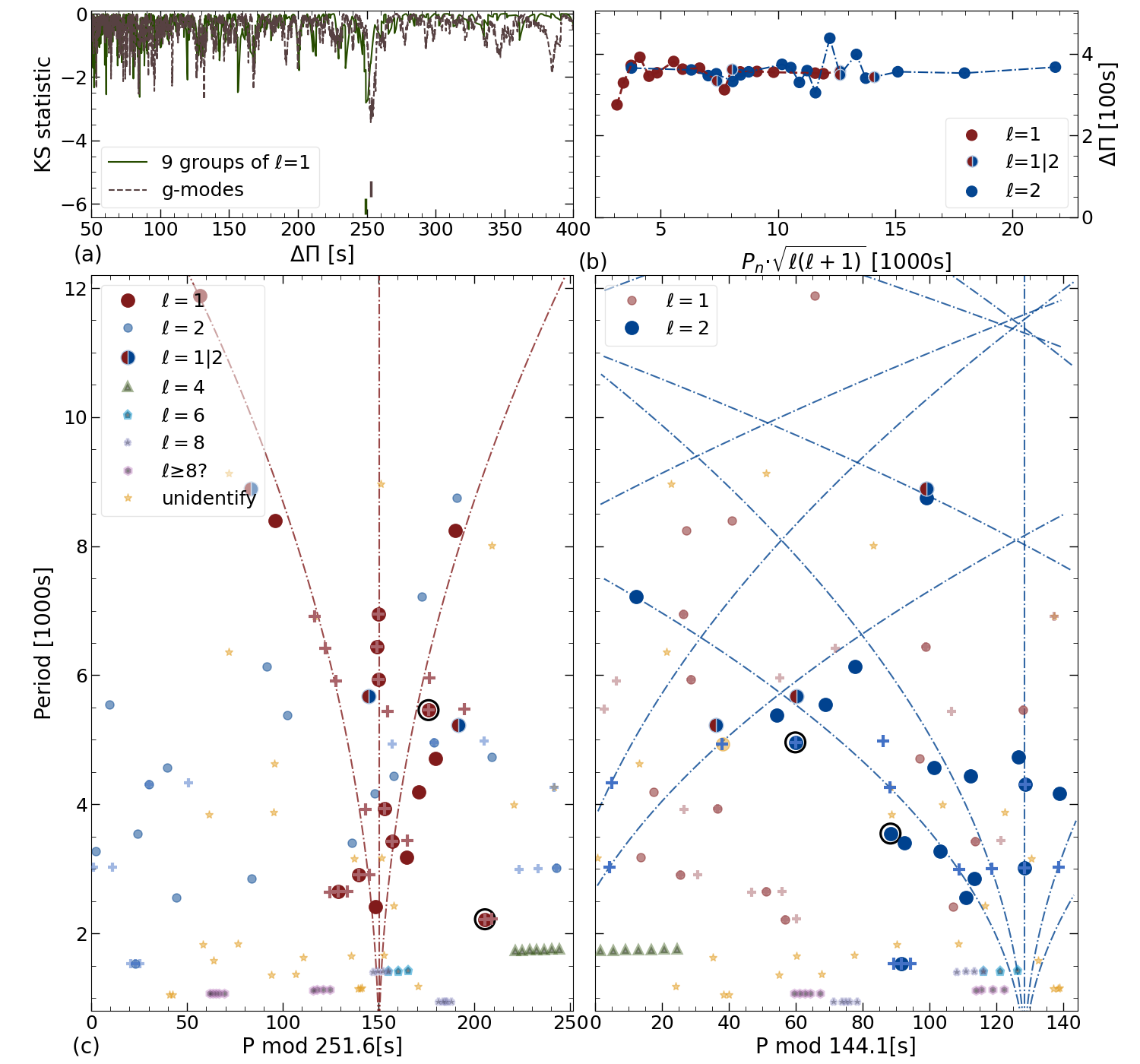
Figure 11: Period spacing and mode identification for independent g-modes. (a) Kolmogorov-Smirnov (KS) tests on two period sets with $\ell=1$. Two vertical segments locate the minimum values for preliminary spacing. (b) Period difference between consecutive modes of the $\ell=1$ and $\ell=2$ sequences, after converting to reduced periods. (c) Échelle diagram for dipole (left) and quadruple (right) modes. The vertical curves represent the corresponding period for rotational components, with 3 and 5 for triplet and quintuplet, respectively. The red and blue + symbols represent the splitting frequency components for $\ell=1$ and $\ell=2$, respectively. And the yellow cycle indicates the mode in $\ell=2$ with a larger deviation in frequency splitting values. The modes surrounded by the solid circles are possibly identified to be trapped modes.

Another technique that helps mode identification relies on the seismic property of periods of g-modes or frequency of p-modes. Here, we only analyzed the property of g-modes as high-frequency p-modes are only a few in PG 0101+039. In the asymptotic limit ($n\gg\ell$), consecutive overtones of g-modes are nearly equally spaced in period (see, e.g., Aerts et al. 2010). The pulsation period of a given mode with degree $\ell$ and radial order $n$ can be expressed as $\Pi_{l,n}\approx n\cdot\Pi_{0}/\sqrt{(l(l+1))}+\epsilon$ where $\Pi_{0}$ is the fundamental radial period and $\epsilon$ is an offset (Unno et al. 1979). The period difference (commonly called period spacing) of two consecutive radial overtones with a given modal degree can be estimated as follows:

$$\Delta\Pi_{l}\equiv\Pi_{l,n+1}-\Pi_{l,n}\approx\frac{\Pi_{0}}{\sqrt{(l(l+1))}},$$ (5)

It is convenient to see that the period spacing of $\ell$ = 2 sequence is relative to $\ell$ = 1 sequence with $\Delta\Pi_{\ell=2}\approx\Delta\,\Pi_{\ell=1}/\sqrt{3}$.

Similar to Ma et al. (2022), we performed the Kolmogorov-Smirnov (KS) test to identify the average spacing of g-modes in PG 0101+039. This popular test returns spacing correlations as highly negative values for the most common spacing in a data set (Kawaler 1988). As identified to be rotational dipole modes, the central components of nine $\ell=1$ multiplets were fed for KS test. Then we applied the second KS test for all the independent frequencies lower than 1200 $\mu$Hz to be probable g-modes. Figure 11(a) shows the results of the KS tests that the minimum values locate around 252.9 s and 249.4 s for the first and second tests, respectively. Both values are consistent with that of dipole modes in many sdB pulsators (see, e.g., Reed et al. 2011; Sahoo et al. 2020).

We identified 21 frequencies to be dipole modes, including 9 central ($m=0$) components, based on the rotation splitting (see Fig.3, a). Similarly, 14 frequencies are identified to be quadruple modes, including four central ($m=0$) ones (see Fig.3(b)). In addition, 35 frequencies can be associated with high degree modes forming seven incomplete multiplets (see Fig.3(c-h)). As the high degree modes are very few, we do not provide any identified results to their radial orders, $n,$ and the azimuthal numbers, $m$, except the frequencies near 574 $\mu$Hz. Besides the above modes, we adopted a preliminary period spacing of 251 s and 145 s to identify the $\ell=1$ and $\ell=2$ modes, respectively, based on the KS test. If a mode is satisfied within the value of less than 35 s and 25 s to the radial order of the $\ell=1$ and $\ell=2$ sequences, respectively, we will classify it to that sequence. We then applied a linear fitting to the identified modes and derived the values of $\Delta\Pi_{\ell=1}=249.2\pm 1.5$ s and $\Delta\Pi_{\ell=2}=146.2\pm 1.7$ s, respectively.

To test the fitting results of the asymptotic period spacing, we then constructed the échelle diagrams for the identified modes. In order to give optimal diagrams, we change the period spacing with a step of 0.1 s relative to $\Pi_{\ell=1}=249.2\pm 3\times 1.5$ s and $\Delta\Pi_{\ell=2}=146.2\pm 3\times 1.7$ s, respectively. The optimal échelle diagrams are chosen by maximum the rotational components close to their calculated values. We finally obtained a period spacing of 251.6 s and 144.1 s for the $\ell=1$ and $\ell=2$ sequences, respectively. Figure 11 (c) shows the échelle diagrams of the two sequences, where the most dipole modes locate very close to the calculated period. We observed five multiplets whose components are consistent with the rotational splittings. We assigned the $m$ value with the identified modes by their location to the closest rotational splitting. We identified 28 $\ell=1$ and 28 $\ell=2$ modes, while 3 may be related to both sequences. All identified modes are listed in columns 9-11 of Table 1 with $\ell$, $m,$ and relative $n$ values. We note that the real radial order $n$ can only be derived through seismic modeling. Figure  11 (b) presents the deviation of period spacing as a function of the reduced pulsation period spacing. We observe a jitter pattern in the $\ell=1$ sequence, which is very common in many sdB stars (see, e.g., Østensen et al. 2014; Sahoo et al. 2020). We note that the échelle diagram does not show any clear pattern of ridge in period spacing. From a theoretical aspect, a young sdB does not develop the regularity in period spacing (Charpinet et al. 2014). PG 0101+039 locates the lower part of g-mode puslating sdB stars on the $\log g-T_{\mathrm{eff}}$ diagram, which indeed indicates that PG 0101+039 is a relatively young sdB star, roughly estimated with an age about 50 Myr after the zero-age extreme horizontal branch (Charpinet et al. 2002b; Fontaine et al. 2012). A more precise age can be foreseen in future modeling.

Appendix D AM and FM comparison from various stamped pixels

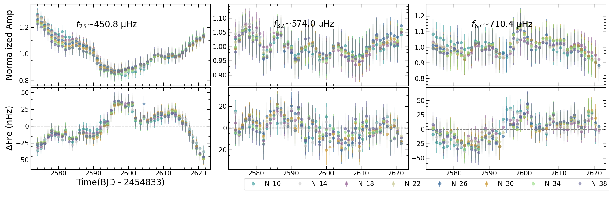
Figure 12: Examples of three frequencies ($f\sim 450.8\,\mu$Hz, $f\sim 574.0\,\mu$Hz and $f\sim 710.4\,\mu$Hz) as a comparison of the amplitude and frequency modulation in PG 0101+039 from stamp-decisive photometry. The sizes of eight types of pixels are labeled in the outside legend. Amplitudes are normalized to units and frequencies are shifted to their averages as represented by the dashed horizontal lines.

As we mention in Section 2.1, the optimal photometry was extracted with a 12-pixel stamp to provide a good number of low-amplitude signals. However, whether the change of stamped size poses a challenge to destroy the intrinsic modulation patterns or not is critical to nonlinear calculation in the future. As documented in Zong et al. (2021), they measured somewhat different patterns of AM between the SAP and PDC-SAP photometry, in particular, a star suffers heavy light pollution from nearby stars. We thus evaluate a similar comparison of different AMs and FMs from the photometry extracted with different sizes of stamped pixels. This step is important for further analysis of the dynamics of oscillation modes in various pulsators from the K2 photometry. During the process of searching for the optimal photometry, we recorded the light curves constructed by various stamps. In our comparison of AM and FM, we again adopted eight of those recording light curves to prewhiten frequencies piecewise in order to save computation time since AM and FM measurements consume the most computational resource. These eight light curves display stamps covering a fraction from 15% to 60% of the entire flux, with pixel sizes ranging from 10 to 38 with a step of four pixels.

The AM and FM were measured from these piecewise light curves that are sliding along the eight recorded light curves with an identical time step of 1 d and window width of 30 d through a similar method to that of Ma et al. (2022) and initialed by Zong et al. (2018). Compared to EPIC 220422705, rotational components can be well resolved in PG 0101+039 since the 30-d length covers more than three times the length of of its rotation period. We note that close peaks within the frequency resolution ($\sim$ 0.4 $\mu$Hz) are detected, we keep the weighted average peak as the measured value for that frequency. There are 35 measurements of AM and FM from the $8\times 48$ constructed light curves. For direct comparison, amplitudes were normalized to their averages and frequencies were shifted to their averages. Figure  12 shows examples of three frequencies as representative results for our comparison. Those three frequencies present various kinds of AM and FM from relatively large scale to small. We clearly see that the patterns of AMs and FMs are consistent within the measuring uncertainties for all eight types of photometry in those three frequencies. For instance, all AM and FM of $f\sim 450.8\,\mu$Hz follow nearly the same trend both in relatively short and long terms. The entire comparison, although not fully provided, gives a similar result to those of the representatives. We, therefore, conclude that both AM and FM patterns do not change when aperture size varies during the extraction of photometry. We note that this conclusion is only valid for targets that are free from contamination by nearby stars. With this test, we can proceed with our characterization of AM and FM in PG 0101+039, without any worries related to the photometric factor.

Appendix E AFMs in PG 0101+039

E.1 AFMs in multiplets

Figure 13 presents the AMs and FMs of the two ($m=-1$ and $m=0$) components forming the $g$-mode doublet near 291 $\mu$Hz. Both the two components exhibit periodic variations of AMs and FMs on timescales approximately of $30-40$ d. By merely comparing the sinusoidal part of the fitting $G_{4}$, the two components display similar scales in AM and FM of $20-30$ ppm and $5-10$ nano Hz, respectively.

Figure 14 displays the AMs and FMs occurring in three components that form the incomplete high degree ($\ell=4$) multiplet near 570 $\mu$Hz. From the sliding LSP, the five components seem stable in amplitude and frequency, whereas the others cannot be distinguished from the noise. Due to the low amplitude in this multiplet, we only measured AMs and FMs for three components ($m=-3,m=-2,m=0$) above our current criteria as revealed by piecewise measurements. With this precision in amplitude and frequency, the behaviors of AMs and FMs have been observed to be variable throughout the entire observation. However, the varying scales both in amplitude and frequency are comparable to their measuring uncertainties of a few tenths of micro Hz or a few ppm. For instance, the FM of the ($m=-2$) component near $f\sim 571.5\,\mu$Hz is a $G_{1}$ fitting but seems periodic if the uncertainties were much smaller. The AMs of $m=-3$ and $m=-2$ evolve nearly in an anti-phase with a parabolic behavior and fitted with a $G_{2}$ function. However, the frequencies of $m=-3$ and $m=0$ seem to evolve in phase with a quasi-periodic behavior on a timescale of approximately 30 days. We note that the AM of the $m=0$ component shows a periodic pattern on a quite short timescale of $\sim 9$ days. However, we also note that this periodic AM has a scale, namely, $\sim 2$ ppm, smaller than the amplitude uncertainties. Similarly, Fig. 15 illustrates the AMs and FMs of two components in the $\ell>3$ multiplet near 707 $\mu$Hz. Both the two FMs exhibit a periodic pattern with a similar timescale of $\sim 30$ days, and a modulating scale of $10-20$ nano Hz. The AMs of $f_{67}\sim 710.4\leavevmode\nobreak\ \mu$Hz seems relatively stable during the observation, whereas the other exhibits quasi-periodic AMs with a scale of $\sim 10$ ppm.

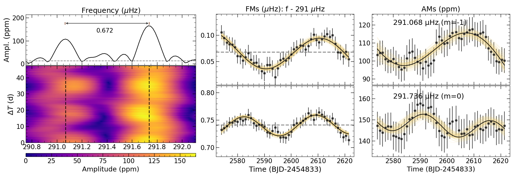
Figure 13: Same as Fig. 6, but for the g-mode doublet near 291 $\mu$Hz.

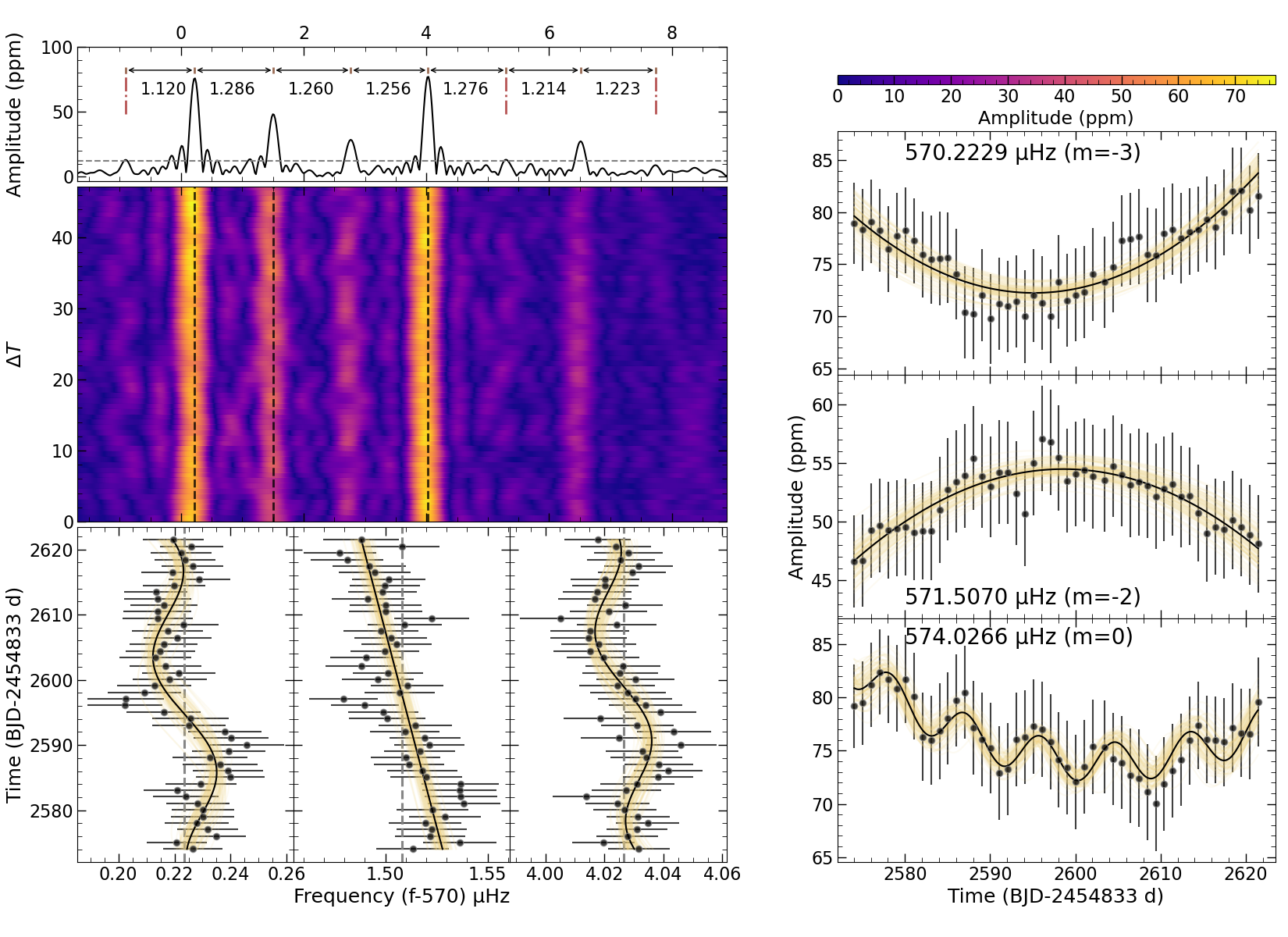
Figure 14: Similar to Fig. 5, but for the $\ell=4$ g-mode multiplet near 570 $\mu$Hz. We note that at least four components are missing in this multiplet and the brown vertical dashed lines indicate the expected position for three of them

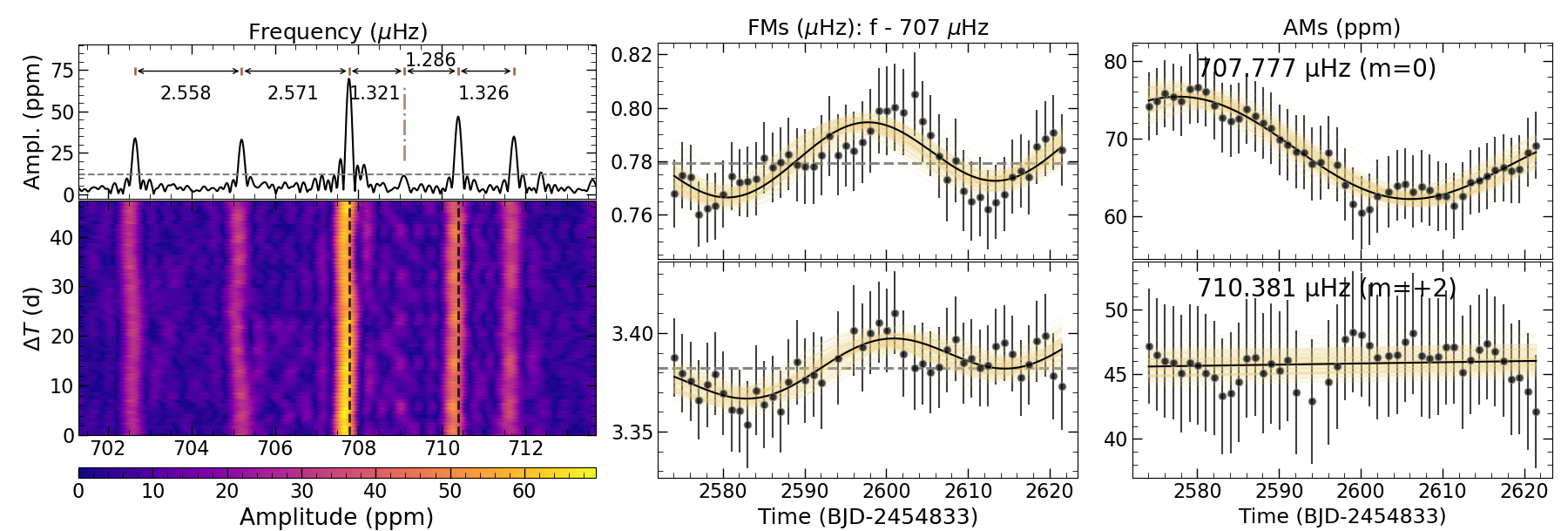
Figure 15: Similar to Fig. 6, but for the $\ell=6$ and $8$ g-mode multiplets near 707 $\mu$Hz.

E.2 The other AFMs

Appendix F Radial velocity information

Table 5: Journal of 50 spectra of LAMOST DR9 and their Radial-velocity (RV) measurements presented in this paper.

Obs. date	BJD	RV	RV error	S/N
2018-10-28	3587.1122	-25.62	2.92	15.5
	3587.1292	-2.07	2.02	13.5
	3587.1459	21.70	3.35	14.3
	3587.1624	24.90	3.09	15.9
	3587.1788	48.67	4.31	13.5
	3587.1954	57.68	2.63	15.7
2019-11-03	3958.1088	-37.57	0.51	81.4
	3958.1250	-22.09	0.62	85.6
	3958.1412	-7.53	0.56	75.0
	3958.1574	9.75	0.73	70.3
	3958.1736	27.71	0.78	69.3
2019-11-08	3963.0716	-81.37	0.48	73.0
	3963.0879	-90.14	0.67	64.2
	3963.1042	-97.06	0.83	63.4
	3963.1204	-98.89	0.87	65.1
	3963.1366	-97.61	0.63	66.3
	3963.1529	-91.85	0.46	66.0
2019-11-11	3966.0807	-32.19	3.35	16.8
2019-11-13	3968.0821	46.57	1.04	47.0
	3968.0983	28.85	0.73	53.4
	3968.1145	6.61	1.03	50.0
	3968.1308	-12.87	0.97	50.4
	3968.1471	-33.32	0.91	44.4
2019-11-18	3973.0914	109.92	0.71	64.6
	3973.1076	111.94	0.66	66.3
	3973.1238	109.69	0.58	61.7
	3973.1400	105.23	0.84	58.4
2019-11-19	3974.0739	-20.39	0.54	79.2
	3974.0901	-3.59	0.65	78.0
	3974.1064	15.86	0.93	77.3
	3974.1226	32.46	0.64	77.9
	3974.1380	47.85	0.86	71.1
2019-12-02	3987.0117	-86.97	0.76	79.4
2019-12-04	3988.9611	53.54	0.91	68.0
	3988.9774	69.65	0.44	67.8
	3988.9936	82.86	0.67	73.2
	3989.0098	93.37	0.64	73.4
	3989.0261	102.53	0.65	70.8
	3989.0423	108.69	0.61	67.1
	3989.0585	110.27	0.68	65.2
	3989.0748	112.07	0.56	60.8
	3989.0910	107.24	1.04	54.3
2019-12-12	3996.9492	61.67	1.18	45.2
	3996.9655	75.38	0.74	49.7
	3996.9817	87.61	0.76	48.2
	3996.9979	96.45	0.98	45.5
	3997.0141	103.78	0.62	46.5
	3997.0304	109.10	0.46	53.9
	3997.0466	110.11	1.34	41.6
	3997.0629	108.36	1.17	35.3