EPTQ: Enhanced Post-Training Quantization via Label-Free Hessian

Abstract

Quantization of deep neural networks (DNN) has become a key element in the efforts of embedding such networks on end-user devices. However, current quantization methods usually suffer from costly accuracy degradation. In this paper, we propose a new method for Enhanced Post-Training Quantization named EPTQ. The method is based on knowledge distillation with an adaptive weighting of layers. In addition, we introduce a new label-free technique for approximating the Hessian trace of the task loss, named Label-Free Hessian. This technique removes the requirement of a labeled dataset for computing the Hessian. The adaptive knowledge distillation uses the Label-Free Hessian technique to give greater attention to the sensitive parts of the model while performing the optimization. Empirically, by employing EPTQ we achieve state-of-the-art results on a wide variety of models, tasks, and datasets, including ImageNet classification, COCO object detection, and Pascal-VOC for semantic segmentation. We demonstrate the performance and compatibility of EPTQ on an extended set of architectures, including CNNs, Transformers, hybrid, and MLP-only models.

1 Introduction

Deep Neural Network (DNN) models are used to solve a wide variety of real-world tasks, such as Image Classification, Object detection, and Semantic Segmentation. However, using such models in day-to-day tasks requires the ability to deploy these models on edge devices. Indeed, in recent years there has been a significant increase in the deployment of DNN models on edge devices. Nevertheless, the deployment of the networks is still challenging, due to their large memory footprint and computational cost.

Many works address this challenge through different techniques, such as designing hardware-dedicated architectures [16, 6, 5], pruning [10, 21, 23, 50], and quantization [2, 3, 29, 15]. Here, we focus on quantization, an effective way to reduce the model size and computational cost by converting the weight and activation tensors to low bit-width representation.

There are roughly two main distinct approaches for quantizing a neural network model. The first one is Post-Training Quantization (PTQ) [4, 25, 19, 30, 47], which solely performs a small statistics collection to determine the quantization parameters without the need for labeled data. The benefit of PTQ is that it is usually simple and fast. However, this approach might suffer from high accuracy degradation. The second approach is Quantization-Aware Training (QAT) [17, 26, 18, 13, 38] in which the model parameters are retrained (with labeled data) to reduce the quantization-induced error. QAT usually obtains better accuracy than PTQ but at the cost of computational and algorithmic complexity, as well as the requirement for the availability of the whole training data.

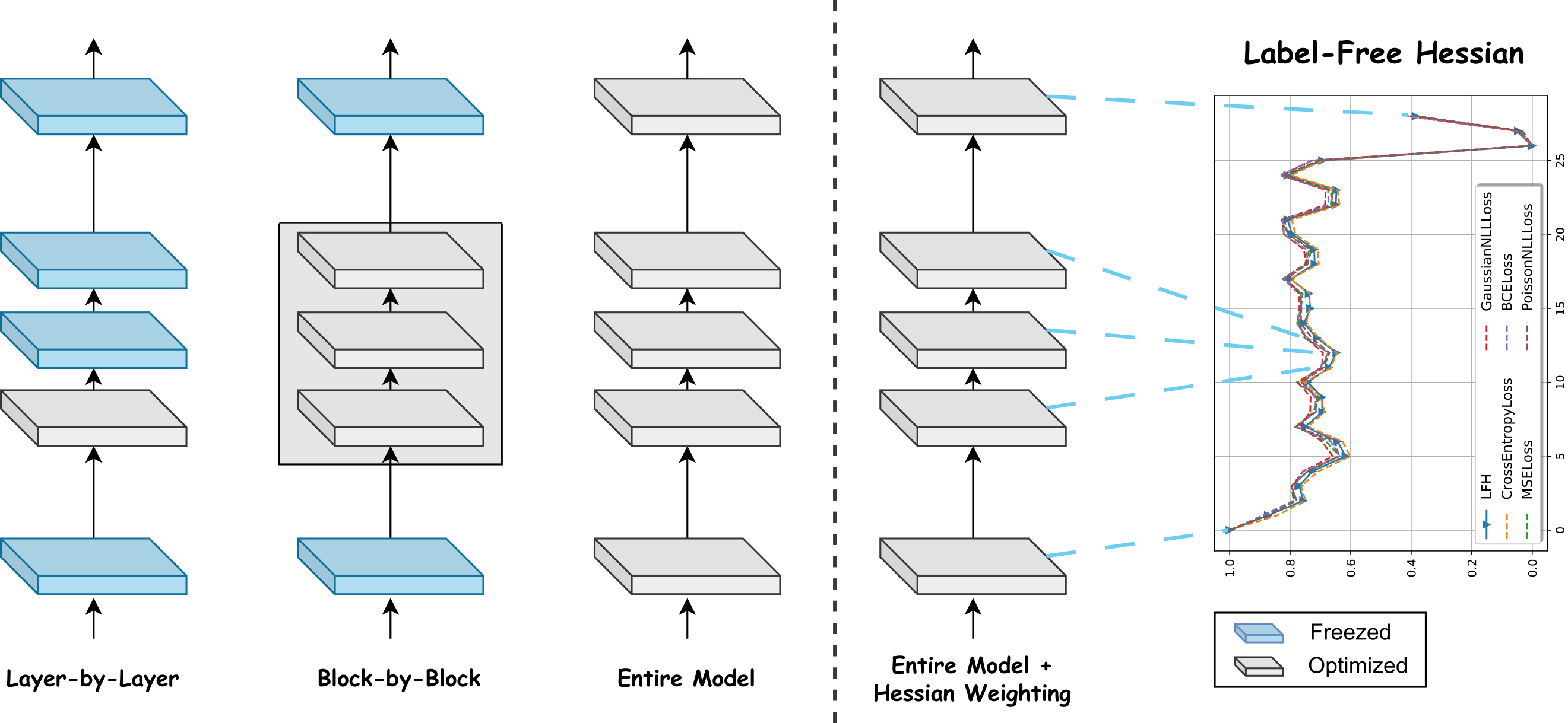
Figure 1: Overview of several quantization optimization techniques compared to EPTQ. EPTQ optimizes the entire network at once, but uses Hessian weighting to give attention to layers that are more sensitive to quantization during the optimization process.

Recent methods, such as AdaRound [36], BRECQ [30], AdaQuant [25], and QDrop [45], present a compromise between PTQ and QAT, by applying a short optimization process without the need for labeled data. These approaches are based on optimizing the error between the floating point model and the quantized one. The main difference between the existing methods is the optimization process itself, as demonstrated in Figure 1. In AdaRound, the optimization is done layer-by-layer, whereas AdaQuant optimizes the entire network simultaneously. BRECQ shows that block-by-block optimization can achieve better results than both. However, a block-by-block approach requires a manual selection of layers on which the optimization is performed.

In this work, we remove the manual layers selection process, while keeping the accuracy benefits of BRECQ. To this end, we define a new objective that captures the sensitivity to quantization of each of the quantized layers. Intuitively, we would like to provide greater attention to layers for which the quantization error will cause a larger change in the task loss. A known metric that captures this information is the Hessian trace, which is widely used in many model compression and optimization works [12, 11, 49, 50]. However, computing the Hessian of a task loss function requires labels, which is unsuitable for PTQ.

To overcome the aforementioned challenges, we suggest Enhanced Post-Training Quantization (EPTQ), an adaptive knowledge distillation method. EPTQ automatically enforces attention on the important layers, which helps to improve the optimization process. In order to provide such attention, we propose Label-Free Hessian (LFH), a new technique for approximating the Hessian trace of the task loss without labeled data. A demonstration of the EPTQ optimization scheme, compared to the other aforementioned techniques, is depicted in Figure 1.

We present state-of-the-art results on various networks, tasks, and datasets without the necessity of manually selecting points for performing the optimizationlayers on which the optimization is performed. Moreover, we demonstrate EPTQ in a mixed precision quantization scheme to obtain further improved accuracy.

In particular, our contributions are the following:

1. We propose an optimization method for post-training quantization, named EPTQ, which is model-agnostic and based on knowledge distillation with adaptive weighting.

2. We introduce a new method, named Label-Free Hessian, to approximate the Hessian trace of the task loss, without the use of labeled data.

3. We present state-of-the-art results using EPTQ to quantize a wide variety of tasks (Image Classification, Semantic Segmentation, and Object Detection), architectures (CNNs, transformers, hybrid, and MLP-only), and datasets (ImageNet, COCO, and Pascal VOC). We also incorporate mixed precision search into our method to obtain improved accuracy under memory restrictions.

In the spirit of reproducible research, the code of this work is available at [40] and implemented inside Model Compression Toolkit (MCT) https://github.com/sony/model_optimization.

2 Related Works

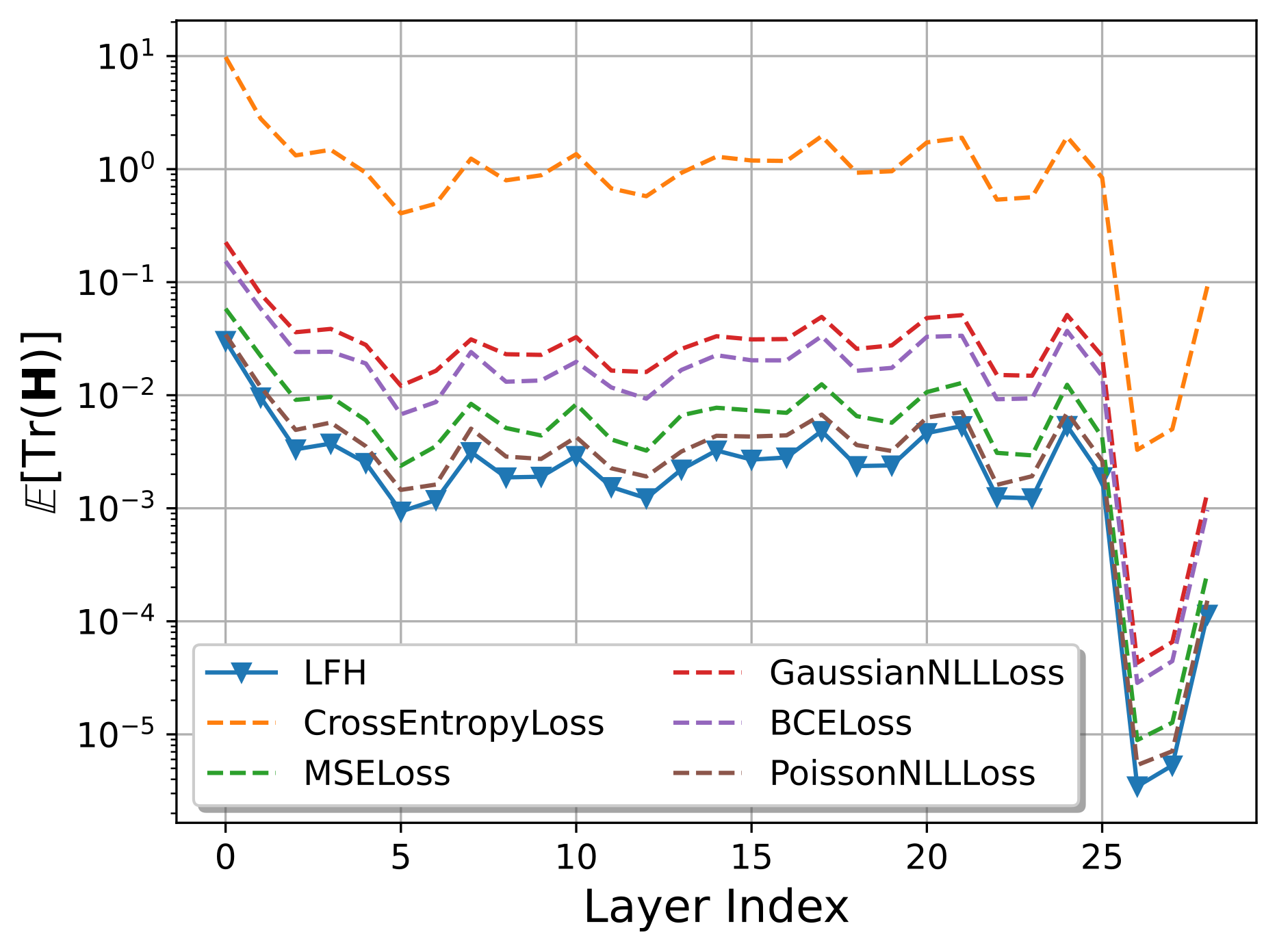
(a) Unnormalized

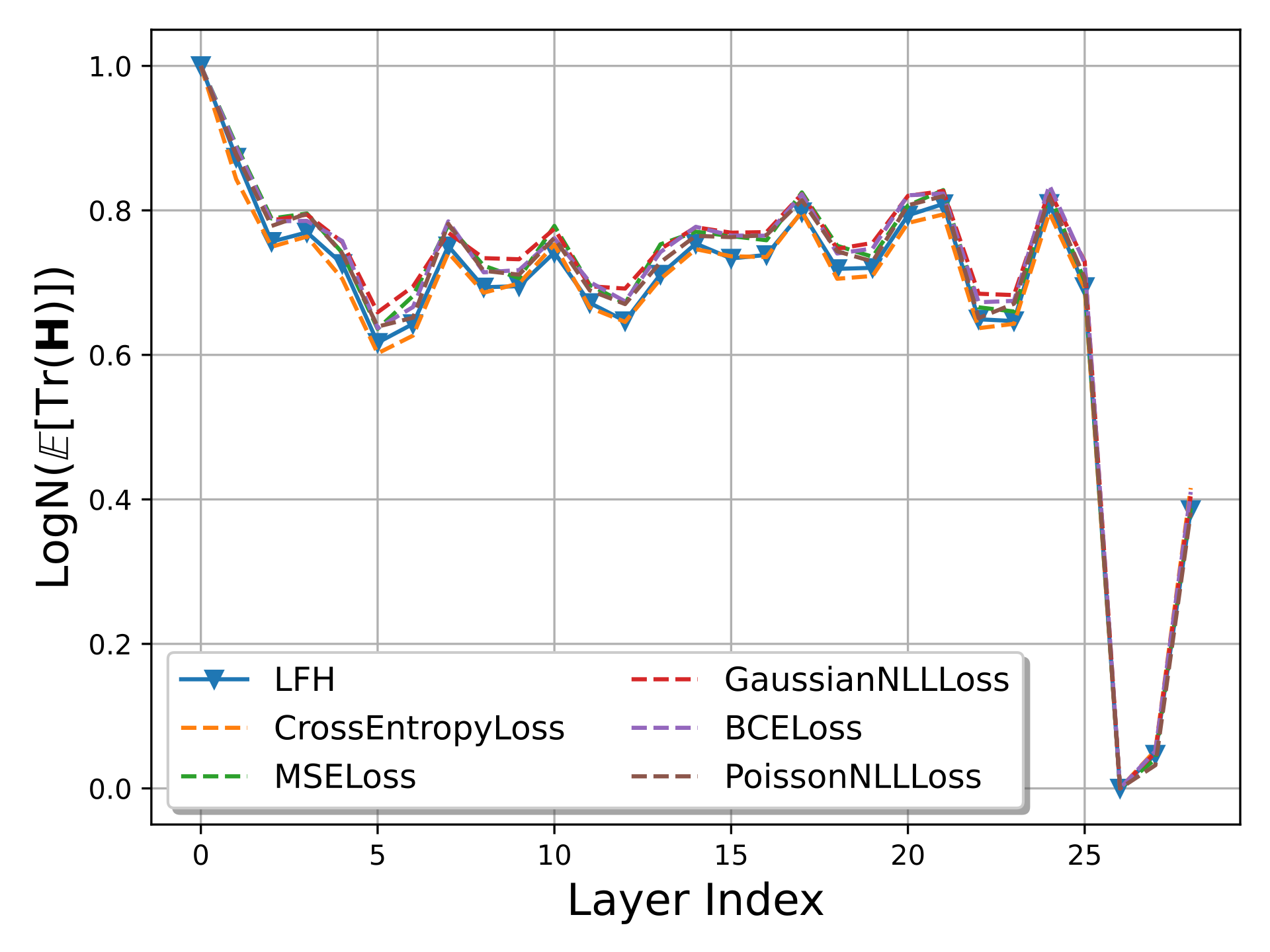
(b) Normalized

Figure 2: Comparison between LFH and the true Hessian trace [49] of different loss functions on ResNet18 without (1) and with (2) log-normalization, on random ImageNet samples.

2.1 Post-Training Quantization Optimization

Recently, there have been many advances in PTQ strategies. Several methods that received a lot of attention are layer-by-layer and block-by-block optimization. A layer-by-layer PTQ approach was first introduced in AdaRound [36]. By investigating the second-order term in the Taylor series expansion of the task loss, it is shown that the common rounding-to-nearest quantization method is sub-optimal w.r.t. the task loss. Instead, the rounding policy is learned by optimizing a per-layer local loss.

AdaQuant [24] follows AdaRound and relaxes its implicit constraint, which forces the quantized weights to be within ${\pm 1}$ of their round-to-nearest value. Another leap was achieved in BRECQ [30], which leverages the basic building blocks in neural networks and reconstructs them one by one. It allows a good balance between cross-layer dependency and generalization error. In addition, BRECQ makes a comprehensive theoretical study of the second-order error of the loss induced by quantization, which is then used to improve the optimization process.

Furthermore, these optimization methods utilize knowledge distillation [22, 35, 41, 48], where the information from the floating point model is used to guide the quantized model. Another example of using knowledge distillation for quantization is QAT-QKD [28], which proposes a combination of self-studying, co-studying, and tutoring methods to effectively apply model quantization using knowledge distillation.

2.2 Hessian for Model Compression

Most model compression methods, such as quantization and pruning, require some assessment of the sensitivity of each part of the model that is being modified. One popular method, originally introduced in HAWQ [12], is to use second-order information to assess the quantization sensitivity of each block. The authors suggest computing the eigenvalues of the Hessian matrix of the model’s task loss with respect to the parameters of each block. The authors then use the eigenvalues to perform mixed precision quantization, a known quantization method, in which varying bit-widths are assigned to different layers of the network. Q-BERT [43] adopts the idea of using the eigenvalues of the Hessian matrix and applies it to a transformer-based architecture in order to quantize it to very low precision. HAWQ-V2 [11] and HAWQ-V3 [48] further extend the idea and use the trace of the Hessian matrix to assess the sensitivity of each block. The Hessian trace provides a better assessment of the sensitivity of each block. Thus, it helps to improve the mixed precision quantization process.

A similar idea is also used for structured pruning in several works. OBS [20] and L-OBS [10] compute the Hessian inverse and use it to suggest an improved pruning mechanism. HAP [50] looks at the Hessian as a block diagonal operator, which allows to solve issues that are not considered in the pruning methods of the other works.

Nonetheless, computing the Hessian information is usually infeasible, due to the very large size of the Hessian matrix. Hence, different algorithms are used to approximate the necessary Hessian information. For example, a recent work named PyHessian [49] introduces a framework for computing different Hessian metrics for neural networks, such as Hessian eigenvalues, trace, and spectral density.

3 Method

We introduce an Enhanced Post-Training Quantization (EPTQ) method that enables to remove the necessity of manually selecting layers on which the optimization is performed. We aim to achieve this without sacrificing the benefits of a wise manual layer selection. We obtain this by utilizing a novel adaptive knowledge distillation objective.

Similarly to prior-art [25, 36, 30], we run a short optimization process that is designed to apply small perturbations to the network’s quantized weights to compensate for the accuracy degradation induced by quantization. We perform the optimization on the entire model at once and regain accuracy by applying an adaptive weighting on the quantization error of each layer, to construct the optimization objective, as demonstrated in Figure 1. Using a newly proposed technique for computing Label-Free Hessian trace, the objective guides the optimization towards focusing on the more sensitive layers, eliminating the necessity of manually selecting the layers on which the optimization is performed.

3.1 Label-Free Hessian

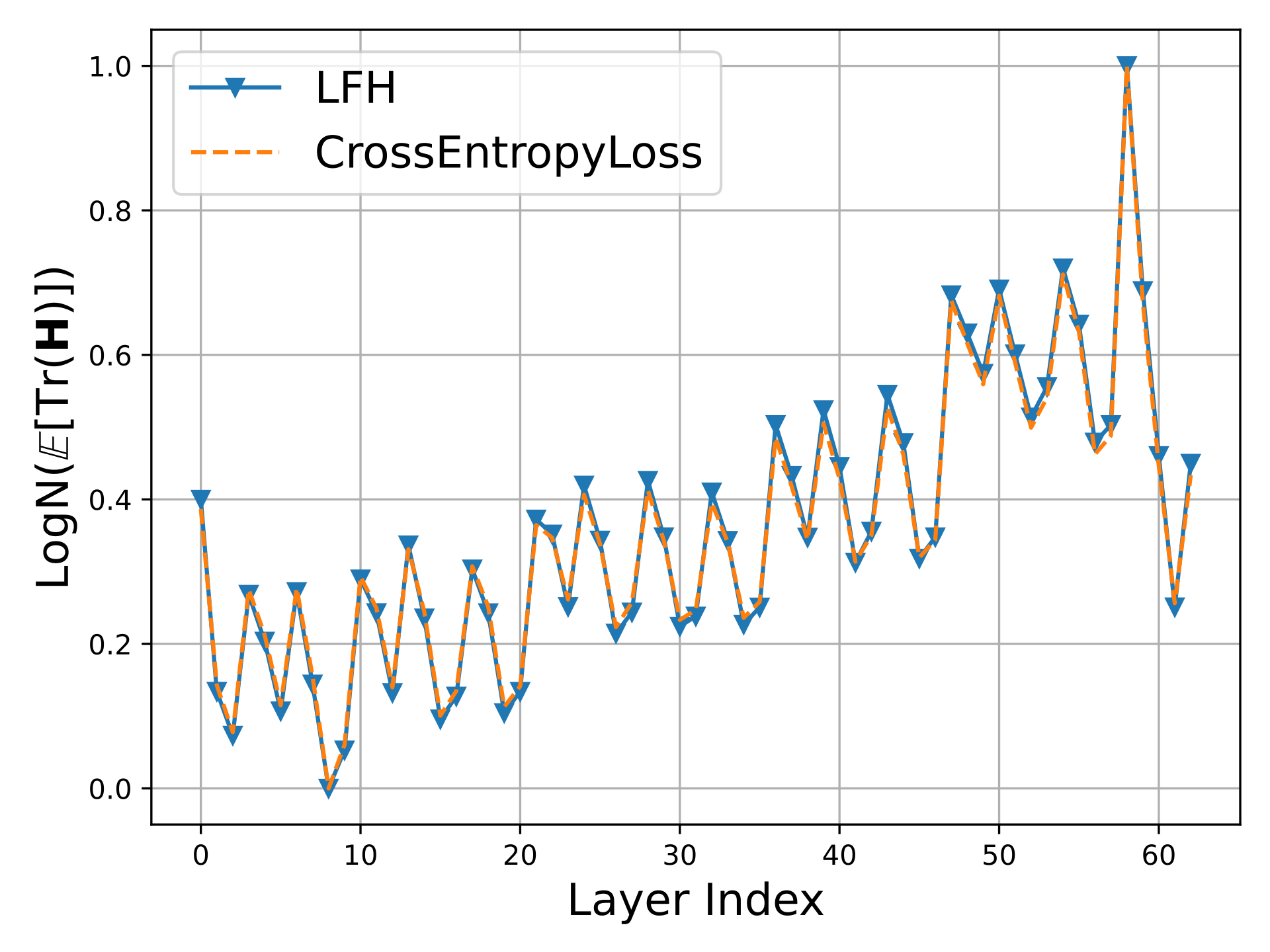
(a) MobileNet-V2

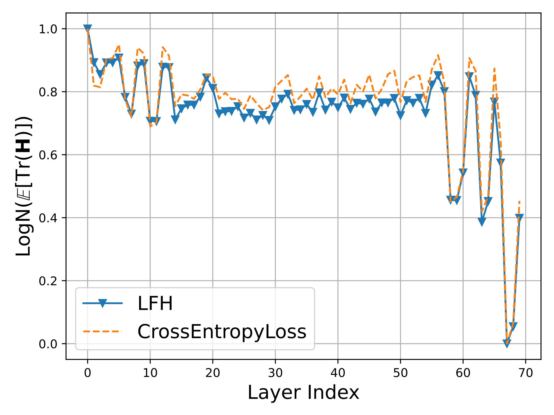
(b) ResNet50

Figure 3: A comparison between the Hessian trace of common task loss functions and our task-invariant Label-Free Hessian approximation on MobileNet-V2 and ResNet50, computed on a random set from ImageNet.

Using the Hessian trace of a neural network task loss to assess a layer’s sensitivity is a well-known technique achieving state-of-the-art results for network quantization [12, 11, 49]. Specifically, let ${f:\mathbb{R}^{d_{i}}\xrightarrow{}\mathbb{R}^{d_{o}}}$ be a neural network and ${\mathcal{L}_{task}}:(\mathbb{R}^{d_{o}},\mathbb{R}^{d_{o}})\xrightarrow{}\mathbb{R}$ be its task loss. Then, the Hessian of the task loss $\mathbf{H}_{\bm{z}}\in\mathbb{R}^{d_{k}\times d_{k}}$ w.r.t. some activation tensor ${\bm{z}\in\mathbb{R}^{d_{k}}}$ is given by:

$${\mathbf{H}_{\bm{z}}}\triangleq{\mathbb{E}_{\bm{y},\bm{x}}\left[\frac{\partial^{2}\mathcal{L}_{task}\left(\bm{y},f\left(\bm{x}\right)\right)}{\partial\bm{z}\partial\bm{z}^{T}}\right]},$$ (1)

where $\bm{x}\in\mathbb{R}^{d_{i}}$ and $\bm{y}\in\mathbb{R}^{d_{o}}$ are the input and label vectors, respectively.

However, computing the exact Hessian is usually infeasible, since it is computed based on the original objective function and thus requires a dataset with labels. To overcome the requirement of a labeled dataset, we leverage the fact that the label vector is omitted during differentiation for many loss functions. We provide examples of such loss functions, such as Cross-Entropy and Mean-Squared Error, and the expression of their Hessian w.r.t. the model output in Appendix C.1. As a result, the Hessian of the task loss w.r.t. the model’s output is independent of the label vector. Using this insight we present Label-Free Hessian (LFH):

Theorem 3.1 (Label-Free Hessian).

Assume that a network model $f$ minimizes a task loss $\mathcal{L}_{task}$ and the following assumption is satisfied $\forall i,j$:

$$\mathbb{E}_{\bm{y},\bm{x}}\left[\left.\nabla_{\bm{r}}\mathcal{L}_{task}\left(\bm{y},\bm{r}\right)\right|_{\bm{r}=f\left(\bm{x}\right)}\bm{u}_{i,j}\left(\bm{x}\right)\right]\approx 0,$$ (2)

where $\left[{\bm{u}_{i,j}\left(\bm{x}\right)}\right]_{k}=\frac{\partial^{2}\left[{f\left(\bm{x}\right)}\right]_{k}}{\partial\left[{\bm{z}}\right]_{i}\partial\left[{\bm{z}}\right]_{j}}$ is the $i^{th}$, $j^{th}$ element of the model’s Hessian matrix w.r.t. its $k^{th}$ output. In addition, assume that the Hessian of the task loss ${\mathbf{B}\left(\bm{y},\bm{r}\right)=\frac{\partial^{2}\mathcal{L}_{task}\left(\bm{y},\bm{r}\right)}{\partial\bm{r}\partial\bm{r}^{T}}}$ w.r.t. the model’s output $\bm{r}$ is independent of the label vector $\bm{y}$ and therefore can be denoted by $\mathbf{A}\left(\bm{r}\right)$. Then, the Hessian trace of the task loss w.r.t. activation tensor $\bm{z}$ of $f$ is approximated by:

$$\mathrm{Tr}\left(\mathbf{H}_{\bm{z}}\right) \approx$$ (3)

$$\mathbb{E}_{\bm{x}}\left[\mathrm{Tr}\left(\mathbf{J}_{\bm{z}}\left(\bm{x}\right)^{T}\left.\mathbf{A}\left(\bm{r}\right)\right|_{\bm{r}=f\left(\bm{x}\right)}\mathbf{J}_{\bm{z}}\left(\bm{x}\right)\right)\right],$$

where $\mathbf{J}_{\bm{z}}\left(\bm{x}\right)=\frac{\partial f\left(\bm{x}\right)}{\partial\bm{z}}$ is the Jacobian matrix of the model’s output w.r.t. $\bm{z}$.

A detailed proof of Theorem 3.1 is given in Appendix B.

According to Theorem 3.1, we can dispose of the necessity of a labeled dataset. Instead, we replace it with an approximation of the trace of the squared Jacobian matrix w.r.t. the layer’s output activation tensor. In order to use Theorem 3.1 to approximate the Hessian trace, it is required that: (1) the Hessian of the task loss ${\mathbf{B}\left(\bm{y},\bm{r}\right)}$ would be independent of the label vector $\bm{y}$, and (2) that the assumption specified in Equation 2 would be satisfied. This assumption can often be satisfied if we assume that the model has converged during training, meaning it has almost zero gradients, i.e., $\left.\nabla_{\bm{r}}\mathcal{L}_{task}\left(\bm{y},\bm{r}\right)\right|_{\bm{r}=f\left(\bm{x}\right)}\approx 0$, similar to [12, 36, 30]. This result provides us with the means to closely approximate the Hessian trace without the necessity of a labeled dataset. Note that, while this requirement holds for many common loss functions, Theorem 3.1 would not necessarily give an accurate approximation for loss functions that do not hold it, such as Sharpness-Aware Maximization (SAM) [14].

We further simplify Equation 3 by looking at the empirical Hessian trace of several different loss functions, as shown in Figure 2. We observe that the actual Hessian trace of these losses equals each other up to a scale. This motivates us to ignore the specific task loss (in addition to removing the dependency on a labeled dataset), by using only the trace of the squared Jacobian matrix. As a result, we get that:

$$\mathrm{Tr}\left(\mathbf{H}_{\bm{z}}\right)=c\cdot\mathbb{E}_{\bm{x}\sim\mathcal{D}_{R}}\left[\mathrm{Tr}\left(\mathbf{J}_{\bm{z}}\left(\bm{x}\right)^{T}\mathbf{J}_{\bm{z}}\left(\bm{x}\right)\right)\right],$$ (4)

where $\mathcal{D}_{R}$ is a representative dataset of unlabeled samples.

Finally, we wish to correct the scaling gap. Because we are only interested in the relative information between the Hessian traces of different layers we can use the simplified Hessian trace and correct the scaling gap. Such information can be used for ranking or weighting tensors, as in [11]. Specifically, we consider a model with $n$ layers, where their output activation tensors reside in the set ${\mathcal{Z}=\{\bm{z}_{i}|1\leq i\leq n\}}$.

Given the simplified Hessian trace (Equation 4) of all layers in the set $\mathcal{Z}$, we apply log normalization on the Hessian traces, which is done as follows: let ${\bm{w}\in\mathbb{R}^{n}}$ be a vector of the Hessian traces of the activation tensors in ${\mathcal{Z}}$ where ${\left[{\bm{w}}\right]_{i}=\mathrm{Tr}\left(\mathbf{H}_{\bm{z}_{i}}\right)}$, then the following log normalization is applied to the vector $\bm{w}$: $\mathrm{LogN}\left(\bm{w}\right)=\frac{\left(\ln\left(\bm{w}\right)-c_{min}\right)}{c_{max}-c_{min}},$ where ln is an element-wise logarithmic function, and $c_{max}$ and $c_{min}$ are the logarithmic values of $\max\limits_{i}\bm{w}_{i}$ and $\min\limits_{i}\bm{w}_{i}$, respectively. The log normalization corrects the loss shift and closes the gap between the approximation and the actual Hessian trace.

To demonstrate this result, we compare LFH to the actual Hessian values on ResNet18 with several loss functions. Figure 2 presents the results with and without log normalization. Moreover, in Figure 3 we present the LFH on two additional models and compare it with the true Hessian trace. From this comparison, we can see that the normalized LFH is aligned with the true Hessian values in all cases. This demonstrates that LFH can provide a good approximation for the Hessian trace, for common objective functions, without the necessity of labeled data. In practice, the expectation in Equation 4 is computed via empirical mean:

$$\mathrm{Tr}\left(\mathbf{H}_{\bm{z}_{i}}\right)\approx\frac{\sum_{\bm{x}\in\mathcal{D}_{R}}\mathrm{Tr}\left(\mathbf{J}_{\bm{z}_{i}}\left(\bm{x}\right)^{T}\mathbf{J}_{\bm{z}_{i}}\left(\bm{x}\right)\right)}{|\mathcal{D}_{R}|},$$ (5)

where $|\mathcal{D}_{R}|$ is the size of the representative dataset.

Finally, we provide a modification of the Hutchinson algorithm [49, 1] for a fast approximation of the trace of the Jacobian matrix norm (Appendix C.2). This modification eliminates the need for computing the Jacobian matrix, which can be very costly.

3.2 Post-Training Quantization Via Hessian-aware Knowledge Distillation

We introduce EPTQ, an enhanced PTQ method that utilizes LFH in knowledge distillation [22, 35] to transfer knowledge from the floating-point model to the quantized model. We utilize the symmetric quantizer from [36], which updates the rounding value of the quantized weights between the floor and ceiling points. Specifically, let $\mathbf{\Theta}$ be the set of parameters to be optimized, that is, the set of variables ${V=\{V_{i}\}_{i=1}^{q}}$ and the quantization step size for each of the $q$ quantizers. In addition, we add the biases of each layer to $\mathbf{\Theta}$ as well.

Let $\mathcal{Z}$ be as defined in Section 3.1, that is, a set of tensors of interest, on which we compute the distillation loss. We denote $\bm{z}_{ij}$ and $\tilde{\bm{z}}_{ij}\left({\mathbf{\Theta}}\right)$ as the $i^{th}$ activation tensors when taking sample $j$ as the input for the float and quantized networks, respectively. Then, we define the Hessian-aware knowledge distillation objective as follows:

$$\mathcal{L}_{KD}\left(\mathbf{\Theta}\right) =\sum_{i=1}^{n}\bm{w_{i}}\cdot\sum_{j=1}^{k}\left\lVert\bm{z}_{ij}-\tilde{\bm{z}}_{ij}\left({\mathbf{\Theta}}\right)\right\rVert_{\mathrm{F}}^{2}$$ (6)

$$+\lambda\cdot f_{reg}(V),$$

where $n$ is the number of activation tensors on which we measure the distance, $k$ is the number of images in a batch that are used for computing the distance metric, $\bm{w_{i}}$ is the LFH trace value of the $i^{th}$ activation tensor, and $\left\lVert\mathbf{A}\right\rVert_{F}$ is the Frobenius norm of tensor $\mathbf{A}$ [42]. The term ${f_{reg}(V)}$ is a regularization factor that encourages the optimization to converge towards rounding the quantized values either up or down. The way to make the optimization converge to one of the extremes is by performing an annealing process, which is detailed in [36]. The last parameter $\lambda$ is a regularization hyper-parameter.

The use of LFH allows us to provide greater attention to the quantization error induced by activation tensors that cause a bigger change to the task loss. Moreover, the loss in Equation 6 does not require prior knowledge of the network’s structure since it is encapsulated in $\bm{w_{i}}$.

Furthermore, we integrate a mixed precision search, where each weight or activation quantizer can have a different precision out of a set of options $\mathcal{B}$, such that the quantized model will satisfy a set of hardware constraints (e.g., memory, power, and latency). The hardware constraints used in this work are described in Section 4.2. For the mixed precision search, we use a well-known method [7, 24, 47] that is based on Integer Linear Programming, which is detailed in Appendix D. The general guideline of our method is described in Algorithm 1. Note that in the algorithm, $n$ represents the number of comparison pointslayers in the model, as detailed in Section 3.1. Extended details are given in Appendix A.

We illustrate the benefit of our adaptive Hessian-aware weighting compared to the common approach of taking a simple average, i.e., $\bm{w_{i}}=\frac{1}{n}\forall i$. We measure the accuracy of several models using two weighting approaches with weights quantized to 3 bits. The results are presented in Table 1.

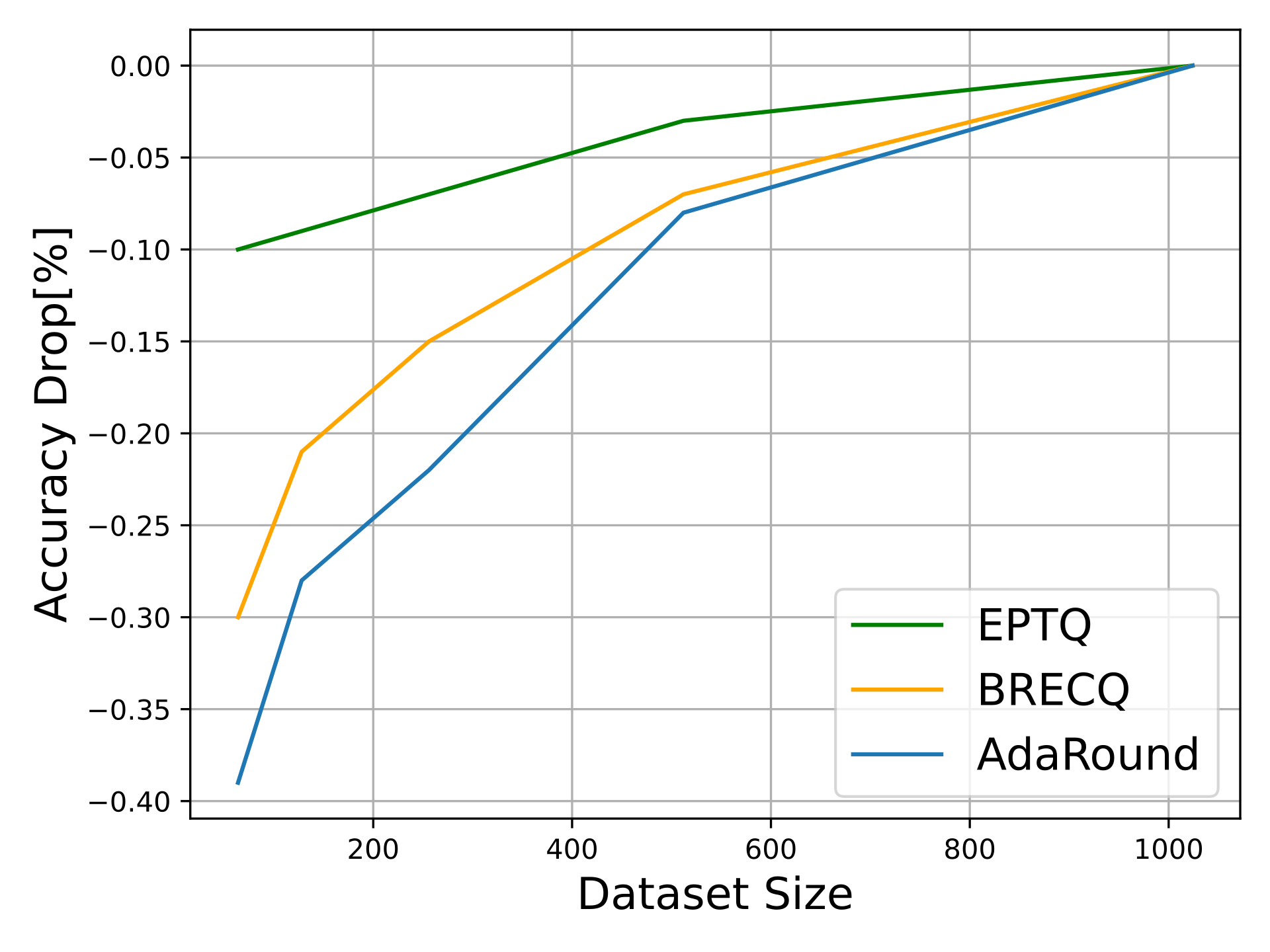
Figure 4: Accuracy drop due to a change in the dataset size on ResNet18 with 4-bit weight and 8-bit activation quantization. The accuracy drop is relative to the results with 1024 samples.

It can be seen that using the Hessian-aware weighting improves the accuracy of all of the presented models compared to the simple average method. In addition, we note that the execution time of the complete quantization process is relatively short, e.g., about 3 hours for quantizing ResNet18 in single precision on NVIDIA GeForce RTX 3090 GPU, with 80K optimization iteration (the run-time is reduced to about 45 minutes with 20K iterations).

Table 1: The top-1 accuracy of 3-bit weight quantization of several classification networks, with and without Hessian-aware weighting.

Weighting Method	Models
	ResNet18	ResNet50	MobileNet-V2	RegNet-600MF
Average	68.635	74.802	70.02	71.72
LFH	68.73	75.16	70.12	72.1

Finally, we emphasize that in addition to lifting the need for labeled data, our experiments show that the given dataset $\mathcal{D}_{R}$ does not need to be very large for obtaining good optimization results. This point is demonstrated in Figure 4, which shows the accuracy drop due to a change in the dataset size on ResNet18. It implies that changing the number of samples that are used for the optimization does not have a noticeable effect on the results, and a close-to-best accuracy can be achieved even with a reduced dataset size (the delta between the results when using 1024 samples compared to only 64 samples are less than $0.1\%$ in accuracy).

4 Experimental Results

In this section, we perform extensive numerical experiments to validate EPTQ (Section 3). We show that using the adaptive Hessian-aware objective loss achieves competitive, and frequently state-of-the-art results for most of the experimented cases.

We use a representative dataset with 1,024 i.i.d samples for all experiments. We perform 80K gradient steps during the optimization to minimize the adaptive knowledge distillation loss (Equation 6). We report the mean and standard deviation of five runs with different initial seeds for each experiment. The weights are quantized per-channel and the activations are quantized per-tensor. The specifications of our PTQ scheme are depicted in Appendix A.1.

In this section, we present results for the compression of different models on ImageNet classification task [9], using (1) a single precision method and (2) a mixed precision method. In addition, in order to demonstrate the benefits and robustness of EPTQ, we test it on two additional tasks–semantic segmentation and object detection, showing that our approach excels beyond image classification. Moreover, we present results on three additional types of architectures: Transformers, MLP-only, and Hybrid Transformers-Convolutions. In most experiments, we use trained models from PyTorch Image Models [46] and torchvision [33], where the weights and the training procedures are available.

Algorithm 1 EPTQ Optimization Workflow

1:  Input: representative dataset $\mathcal{D}$, a pre-trained model $f$.

2:  Batch Normalization Folding.

3:  Initialize quantization step size $\Delta$ for each quantizer by minimizing the Mean-Squared Error (MSE).

4:  Search bit-width $b\in\mathcal{B}$ for each quantizer.

5:  Compute the LFH trace approximation (Equation 5) for each activation tensor $\bm{z}_{i}$ for all $0\leq i<n$.

6:  Optimize $\Theta$ using SGD by minimizing the adaptive loss (Equation 6).

We compare our results with the reported results of several other quantization optimization methods. For each experiment, we present the quantized accuracy (“Q”) and highlight the delta ($\Delta_{\downarrow}$) from the floating-point accuracy (appears next to the model name). For several networks, the compared methods use a different floating-point model with different published accuracy values which are not publicly available. For the sake of a fair comparison, we present the floating-point baseline accuracy (“BL”) as part of the results.

Table 2: Top-1 accuracy comparison of EPTQ and BRECQ [30] on ImageNet classification task. In addition to the superior accuracy results, EPTQ does not require any manual intervention as opposed to BRECQ’s per-block reconstruction.

Method	W/A	ResNet18 (71.08)		ResNet50 (77.00)		MobileNetV2 (72.49)		RegNet-600MF (73.71)
		Q	$\Delta_{\downarrow}$	Q	$\Delta_{\downarrow}$	Q	$\Delta_{\downarrow}$	Q	$\Delta_{\downarrow}$
BRECQ	4/32	70.70$\pm 0.07$	0.38	76.29$\pm 0.04$	0.71	71.66$\pm 0.04$	0.83	73.02$\pm 0.09$	0.69
EPTQ (Ours)		70.83$\pm 0.02$	0.25	76.77$\pm 0.02$	0.23	72.03$\pm 0.05$	0.46	73.19$\pm 0.04$	0.52
BRECQ	3/32	69.81$\pm 0.05$	1.27	75.61$\pm 0.09$	1.39	69.50$\pm 0.12$	2.99	71.48$\pm 0.07$	2.23
EPTQ (Ours)		70.14$\pm 0.04$	0.94	76.07$\pm 0.12$	0.93	70.39$\pm 0.1$	2.1	71.65$\pm 0.07$	2.06
BRECQ	4/8	70.58	0.5	76.29	0.71	71.42	1.07	72.73	0.98
EPTQ (Ours)		70.76$\pm 0.05$	0.32	76.52$\pm 0.04$	0.48	71.89$\pm 0.07$	0.6	72.97$\pm 0.07$	0.74

Table 3: Top-1 accuracy comparison of EPTQ and other quantization methods, on ImageNet classification task.

	W/A	ResNet18 (69.68)		ResNet50 (76.07)		MobileNetV2 (71.72)
		Q	$\Delta_{\downarrow}$	Q	$\Delta_{\downarrow}$	Q	$\Delta_{\downarrow}$
Bias corr	4/8	67.4	2.28	74.8	1.27	-	-
DFQ [37]		38.98	30.7	52.84	23.23	46.57	25.15
AdaRound [36]		68.55	1.13	75.01	1.06	69.25	2.47
EPTQ (Ours)		69.28$\pm 0.05$	0.4	75.54$\pm 0.06$	0.53	70.27$\pm 0.08$	1.45

4.1 Single Precision Quantization

We examine single precision weight quantization for low bit-widths (4 and 3 bits) on different classification networks and compare our results with other recent PTQ methods. Tables 2 and 3 present a comparison with several methods of low bit-width weights quantization, with changing bit-width precision. Note that the experiments in Table 2 are conducted on the models provided by BRECQ [30]. In this case, in addition to the improved delta accuracy achieved by EPTQ for the absolute majority of models and bit-widths, we emphasize that EPTQ does not require any manual selection of comparison pointslayers to perform the optimization on, making it simpler to use. Moreover, in the EPTQ quantization scheme, we quantize the weights and activations of all layers (including the first and last layers), the output tensor of any linear operation without an activation function, and the addition, and concatenation operations. The experiments in Table 3 are conducted on the models from torchvision [33]. EPTQ presents better delta accuracy for this case as well.

Number of optimization iterations In addition, we conducted an ablation study on the effect of the number of optimization iterations on the resulting accuracy. The results for 4-bit weight quantization for several classification networks are presented in Figure 5. As can be seen, there is no significant benefit from increasing the number of iterations, and for most networks, it is sufficient to run the optimization for only 20K iterations.

Table 4: Mean Intersection Over Union comparison for semantic segmentation on DeeplabV3+ for 4-bit weight and 8-bit activation quantization.

Method	Model	BL	Q	$\Delta_{\downarrow}$
DFQ [37]	DeeplabV3+ [8]	72.94	14.45	58.49
HPTQ [19]		75.56	56.71	18.85
AdaRound [36]		72.94	70.86	2.08
EPTQ (Ours)		75.56	73.848	1.71

4.2 Mixed Precision

We quantize several classification networks to different target model sizes using mixed precision. The bit-width options for each quantizer are $\mathcal{B}=\{2,4,8\}$. We apply a total weight memory constraint that is given by: $\sum_{i\in N_{W}}|\mathbf{W}_{i}|\cdot\bm{b}_{i}$, where $N_{W}$ is the sets of indices for the weight quantizers and $\bm{b}_{i}\in\mathcal{B}$. We use a well-known method for the mixed precision search [24, 48] that is based on Integer Linear Programming, and combine it with an objective function taken from [7]. For more details about the mixed precision formulation, see Appendix D.

In this experiment, only weights are quantized in mixed precision, while the activations are quantized using 8 bits. Figure 6 compares a mixed precision quantization between EPTQ and other quantization methods on ResNet18 (a) and RegNet (b). It shows that the accuracy achieved by EPTQ is better than the ones achieved by the compared methods for all model sizes.

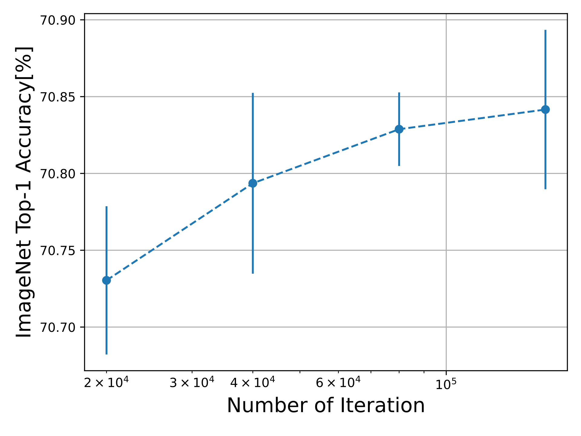
(a) ResNet18

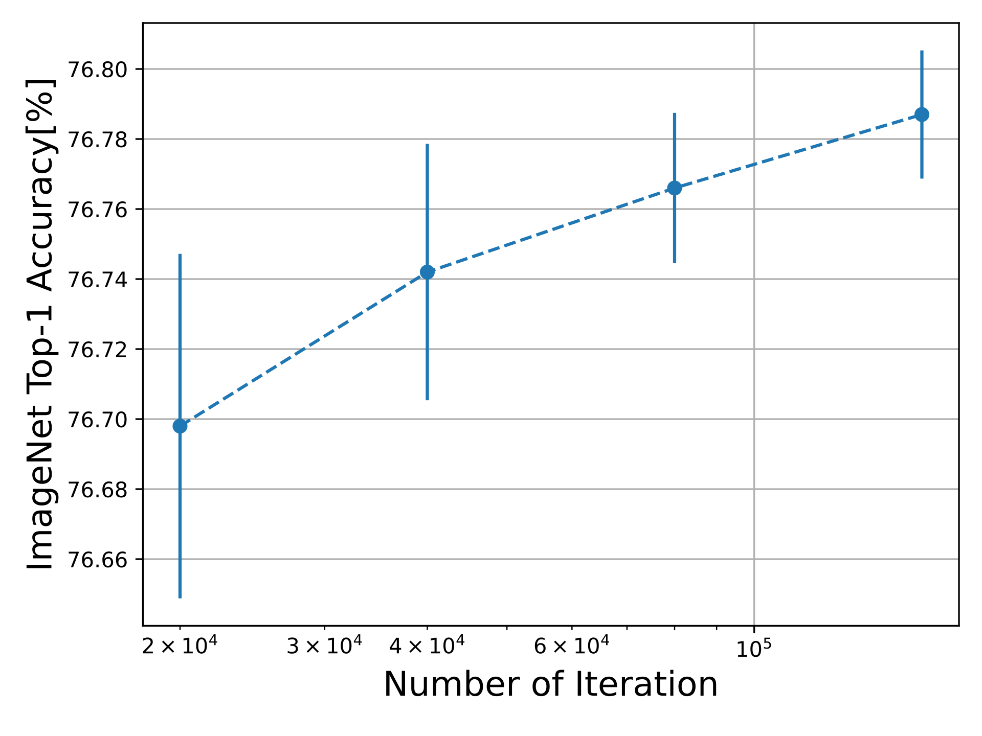
(b) ResNet50

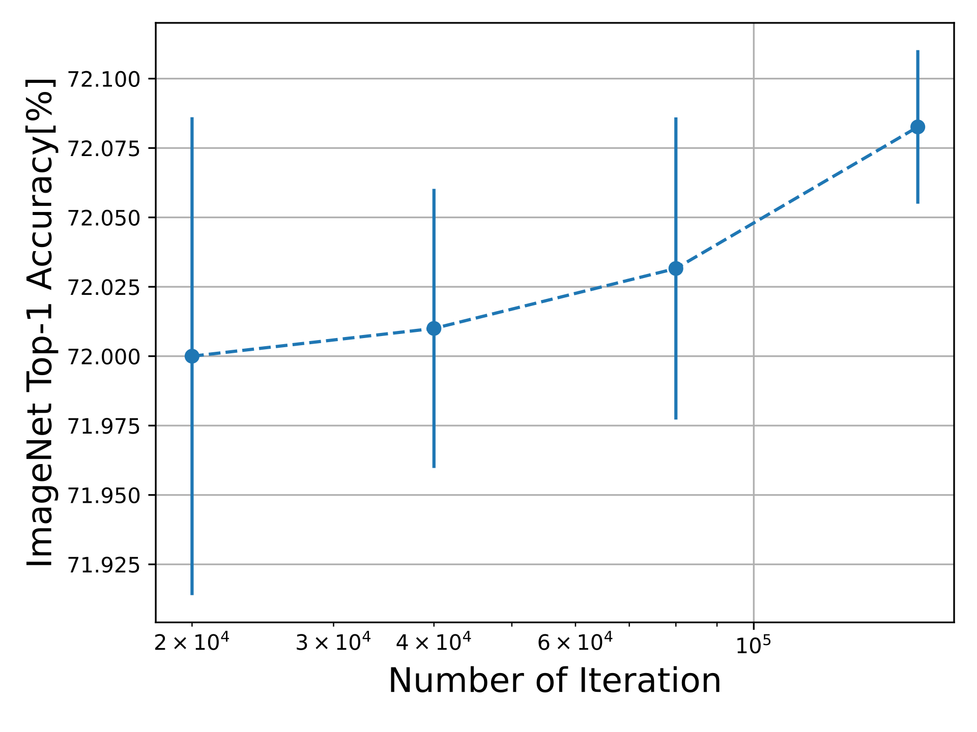
(c) MobileNetV2

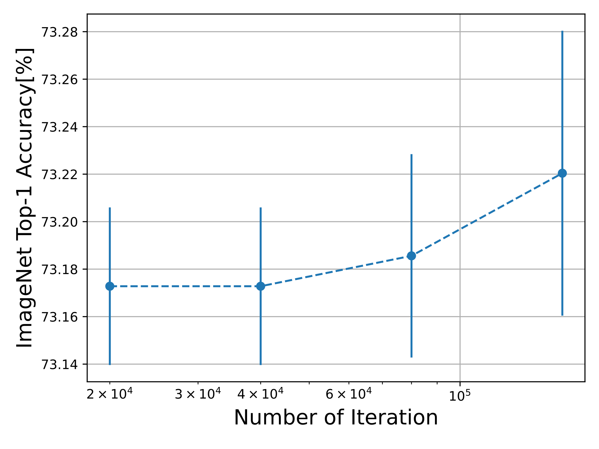
(d) RegNet

Figure 5: Top-1 accuracy of several classification networks quantized with a different number of optimization iterations using 4-bit weights.

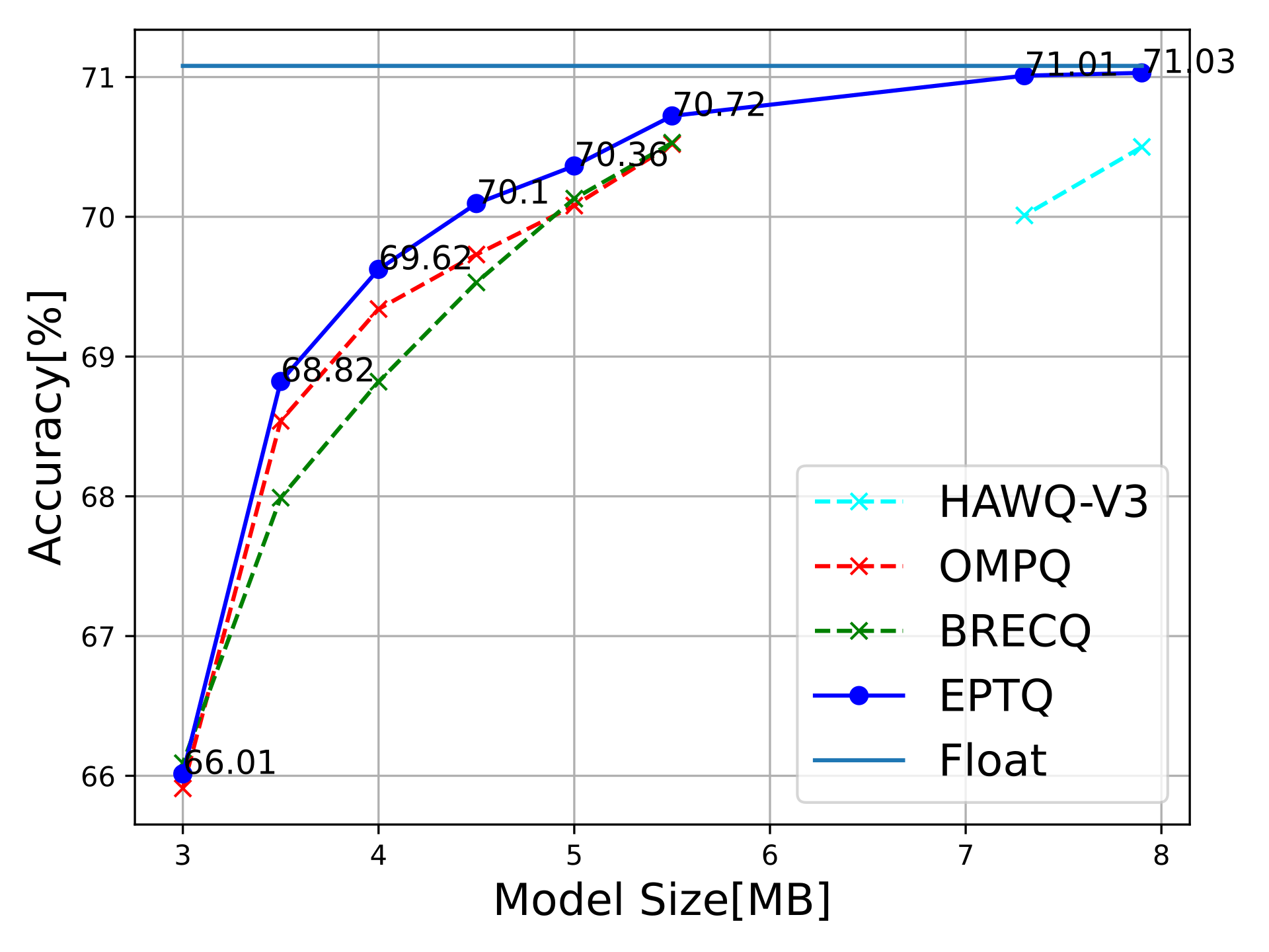
(a) ResNet18

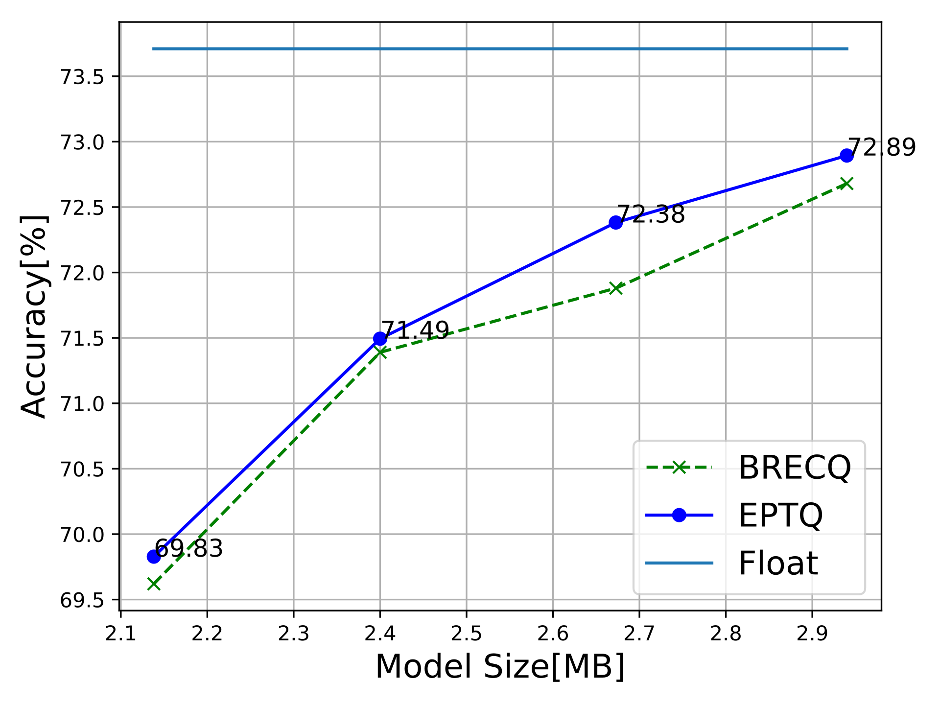
(b) RegNet

Figure 6: Top-1 accuracy of ResNet18 and RegNet. Weights are quantized to different model sizes using mixed precision with $\{2,4,8\}$ bit-width options and activations in 8 bits.

4.3 Additional Results

To demonstrate the benefits and robustness of EPTQ, we experimented it on two additional tasks–semantic segmentation and object detection, showing our approach excels beyond image classification. Moreover, we present results on three additional types of architectures: Transformers, MLP-only, and hybrid Transformers-Convolutions.

Table 5: Mean Average Precision comparison of EPTQ and BRECQ [30] for object detection on RetinaNet network. EPTQ achieves competitive results, despite eliminating the requirement of manually selecting layers for the optimization.

Method	W/A	BL	Q	$\Delta_{\downarrow}$
BRECQ	8/8	36.82	36.73	0.09
EPTQ (Ours)		36.4	36.35	0.05
BRECQ	4/8	36.82	36.65	0.17
EPTQ (Ours)		36.4	36.19	0.21

Table 6: EPTQ Top-1 accuracy of 4-bit weight and 8-bit activation quantization on advanced architectures for image classification.

Model	BL	Q	$\Delta_{\downarrow}$
MobileVit [34]	78.21	77.284	0.92
DeiT-B [44]	83.336	82.85	0.48
Mixer-B/16 [44]	72.7	71.142	1.55

Semantic Segmentation Table 4 presents a comparison between EPTQ and other quantization methods on the DeeplabV3+ [8] model with MobileNetV2 backbone for the semantic segmentation task.

Object Detection Table 5 shows competitive results with BRECQ for quantizing the RetinaNet [31] network with ResNet50 backbone in different precisions, while removing the requirement of manually selecting the comparison points for the optimizationlayers on which we perform the optimization. It can be seen that the benefits of EPTQ are applicable and that it outperforms the state-of-the-art in this task as well.

Additional Architectures Table 6 EPTQ performance on three advanced architectures. Here we examine networks with a different, unique structure, especially compared to the CNNs we tested in the previous experiment. These networks’ structure varies significantly from the constructive block structure of common CNNs, which can cause high ineffectiveness with PTQ optimization methods.

We show that EPTQ effectively runs on such networks and achieves high accuracy for the quantized models, by examining it on the following networks: (1) DeiT [44]–a transformer network; (2) MobileVit [34]–a hybrid network that combines CNNs with vision transformer principles; (3) MLP-Mixer [44]–a network that is composed only of MLP layers as the linear operations. We do a small calibration for some of the hyper-parameters in these experiments, to obtain improved results. To the best of our knowledge, there are no other PTQ methods doing 4-bit weight quantization for these architectures. The results in Table 6 confirm the applicability and high performance of EPTQ on various architectures.

5 Conclusions

In this work, we introduced EPTQ–a post-training quantization method that utilizes knowledge distillation with an adaptive weighting of layers. EPTQ utilizes a new method named Label-Free Hessian (LFH) for approximating the Hessian trace of a neural network’s task loss without the need for labeled data. LFH allows us to effectively produce a weighted objective function for knowledge distillation by giving higher attention to the quantization error induced by activation tensors that cause a larger change to the task loss.

We examined EPTQ on a large variety of DNN models with different architectures and specifications. We conducted experiments on three types of problems: ImageNet classification, COCO object detection, and Pascal VOC semantic segmentation. We showed that EPTQ achieves state-of-the-art results on a wide variety of tasks and models, including ResNet18, ResNet50, MobileNetV2, RegNet and RetinaNet. Additionally, we presented results in a mixed precision quantization scheme which, when combined with EPTQ, allows us to push the accuracy of quantized networks even further.

We believe that the use of LFH is not restricted to EPTQ. As mentioned, other neural network compression techniques, such as pruning, utilize Hessian information to assess the sensitivity of the model’s layers. Such techniques might benefit from incorporating our LFH technique.

Appendix A Post-Training Quantization Scheme

The overall optimization flow, including the mixed precision search, consists of two main stages: (1) Initializing the quantization parameter and bit-width; (2) Optimizing the rounding parameters.

In the initialization stage, we start with a pre-processing step which consists of folding batch normalization layers into their preceding convolution layers. Next, we initialize the quantization step sizes $\Delta$ for all channels for every possible bit-width, i.e., $\Delta_{j}^{(b)}\forall j\in[0,n_{c}-1],\forall b\in\mathcal{B}$, where $n_{c}$ is the number of channels in the network and $\mathcal{B}$ is the set of possible bit-widths. We do it using MSE minimization [39, 19]. Then, we search the bit-width of each quantizer using mixed precision optimizing over different memory metrics, which are described in Section 4.2. This results in a bit-width configuration vector $\bm{b}\in\mathcal{B}^{q}$ where $q$ is the number of quantizers. Note that $q<n_{c}$ since we use per-channel step size and the bit-widths are set per tensor.

Afterward, we begin the optimization of the model parameters where we first compute the attention score, $\bm{u}_{i}\forall i\in[0,n-1]$ using LFH computation. Then, we use gradient descent to minimize the adaptive knowledge distillation loss (Equation  6) over the model parameters $\Theta$.

A.1 Quantization Setting

In this work, we quantized every activation tensor in the neural network accepting fusion between non-linear and convolution. This includes the following quantization points: non-linear, convolution without non-linear, add residual, and concatenation. Note that this differs from other methods like BRECQ [30], which only quantizes part of the neural network activations as stated in [27].

A.2 Hyper-parameter and Training Settings

We use the RAdam [32] optimizer with default parameters and different learning rates for each model with a batch size of $k=32$ samples. All experiments are conducted on an NVIDIA GeForce RTX 3090 GPU. Unless stated otherwise, in all experiments, the following hyper-parameters are used: The optimization learning rate is $lr=3\cdot 10^{-2}$, and the learning rate for the bias and quantization threshold optimization is $10^{-3}$. We set ${\lambda=0.01}$. The Label-Free Hessian is computed using ${\mathrm{Size}\left(\mathcal{D}_{R}\right)=16}$ samples.

Appendix B Label-Free Hessian Theorem Proof

We provide detailed proof for Theorem 3.1.

Proof.

By definition of Hessian and using the chain rule as in [30] we obtain:

$$\left[{\mathbf{H}_{\bm{z}}}\right]_{i,j} ={\mathbb{E}_{\bm{y},\bm{x}}\left[\frac{\partial^{2}\mathcal{L}_{task}\left(\bm{y},f\left(\bm{x}\right)\right)}{\partial\left[{\bm{z}}\right]_{i}\partial\left[{\bm{z}}\right]_{j}}\right]}$$

$$=\mathbb{E}_{\bm{y},\bm{x}}\left[\sum_{k=1}^{d_{0}}\left[{\left.\nabla_{\bm{r}}\mathcal{L}_{task}\left(\bm{y},\bm{r}\right)\right|_{\bm{r}=f\left(\bm{x}\right)}}\right]_{k}\frac{\partial^{2}\left[{f\left(\bm{x}\right)}\right]_{k}}{\partial\left[{\bm{z}}\right]_{i}\partial\left[{\bm{z}}\right]_{j}}\right]+\mathbb{E}_{\bm{y},\bm{x}}\left[\frac{\partial f\left(\bm{x}\right)}{\partial\left[{\bm{z}}\right]_{i}}^{T}\left.\frac{\partial^{2}\mathcal{L}_{task}\left(\bm{y},\bm{r}\right)}{\partial\bm{r}\partial\bm{r}^{T}}\right|_{\bm{r}=f\left(\bm{x}\right)}\frac{\partial f\left(\bm{x}\right)}{\partial\left[{\bm{z}}\right]_{j}}\right].$$ (7)

Using the assumption that $\mathbb{E}_{\bm{y},\bm{x}}\left[\sum_{k=1}^{d_{0}}\left[{\left.\nabla_{\bm{r}}\mathcal{L}_{task}\left(\bm{y},\bm{r}\right)\right|_{\bm{r}=f\left(\bm{x}\right)}}\right]_{k}\frac{\partial^{2}\left[{f\left(\bm{x}\right)}\right]_{k}}{\partial\left[{\bm{z}}\right]_{i}\partial\left[{\bm{z}}\right]_{j}}\right]\approx 0$ we have that:

$$\mathbf{H}_{\bm{z}}\approx\mathbb{E}_{\bm{y},\bm{x}}\left[\mathbf{J}_{\bm{z}}\left(\bm{x}\right)^{T}\left.\mathbf{B}\left(\bm{y},\bm{r}\right)\right|_{\bm{r}=f\left(\bm{x}\right)}\mathbf{J}_{\bm{z}}\left(\bm{x}\right)\right].$$ (8)

Finally, by assumption, $\mathbf{B}\left(\bm{y},\bm{r}\right)$ is independent of $\bm{y}$ and therefore we obtain the required result:

$$\mathbf{H}_{\bm{z}}\approx\mathbb{E}_{\bm{y},\bm{x}}\left[\mathbf{J}_{\bm{z}}\left(\bm{x}\right)^{T}\mathbf{A}\left(\bm{r}\right)\mathbf{J}_{\bm{z}}\left(\bm{x}\right)\right]=\mathbb{E}_{\bm{x}}\left[\mathbf{J}_{\bm{z}}\left(\bm{x}\right)^{T}\mathbf{A}\left(\bm{r}\right)\mathbf{J}_{\bm{z}}\left(\bm{x}\right)\right].$$ (9)

∎

Appendix C Label-Free Hessian Norm

C.1 Loss functions Hessian overview

In Section 3.1 we claim that for many loss functions, the Hessian matrix of the task loss w.r.t. the model output is dependent exclusively on the model output. This implies that we can compute the Hessian without needing to compute the derivative of the original loss function. Here, we prove this claim by presenting a closed-form equation of the Hessian for a set of commonly used loss functions.

It can be observed that for several common loss functions such as Mean-Squared Error (MSE), Cross Entropy with Softmax, Binary Cross-Entropy Sigmoid, Poisson NLL and Gaussian NLL the Hessian is only dependent on the model output. Table 7 shows the corresponding Hessian for each of the aforementioned functions.

Table 7: Loss function with their corresponding Hessian

Loss	Hessian
MSE	$\mathbf{A}\left(\bm{r}\right)=\frac{2}{d_{0}}\mathbf{I}_{d_{0}}$
CE-Softmax	$\left[{\mathbf{A}\left(\bm{r}\right)}\right]_{i,j}=\begin{cases}-\left[{\mathrm{SM}\left(\bm{r}\right)}\right]_{i}\cdot\left[{\mathrm{SM}\left(\bm{r}\right)}\right]_{j},&i\neq j\\ \left[{\mathrm{SM}\left(\bm{r}\right)}\right]_{i}\cdot\left(1-\left[{\mathrm{SM}\left(\bm{r}\right)}\right]_{i}\right),&i=j\end{cases}$
BCE-Sigmoid	$\mathbf{A}\left(\bm{r}\right)=\mathrm{Diag}\left(\mathrm{Sigmoid}\left(\bm{r}\right)\odot\left(1-\mathrm{Sigmoid}\left(\bm{r}\right)\right)\right)$
GaussianNLL	$\mathbf{A}\left(\bm{r}\right)=\frac{2}{\sigma^{2}}\mathbf{I}_{n}$
PoissonNLL	$\mathbf{A}\left(\bm{r}\right)=\mathrm{Diag}\left(\exp\left(\bm{r}\right)\right)$

where $\odot$ is the Hadamard product, $\left[{\mathrm{SM}\left(\bm{x}\right)}\right]_{k}=\frac{\exp\left(\left[{\bm{x}}\right]_{k}\right)}{\sum_{j=1}^{n}\exp\left(\left[{\bm{x}}\right]_{j}\right)}$ is the softmax function, $\mathrm{Sigmoid}\left(x\right)$ is the sigmoid function and $\sigma^{2}$ is the varinace of the Gaussian NLL loss. In Table  7, $\mathrm{Diag}\left(\bm{r}\right)$ denote the transform of vector into a diagonal matrix $\mathbf{D}$ which is defined as:

$$\left[{\mathbf{D}}\right]_{i,j}=\begin{cases}0,&i\neq j\\ \left[{\bm{r}}\right]_{i},&i=j\end{cases}$$

We provide a detailed proof of the Hessian computation of the loss functions presented in Table 7.

Proof.

Denote the label vector as $\bm{y}\in\mathbb{R}^{d_{0}}$ and the prediction vector as $\bm{r}\in\mathbb{R}^{d_{0}}$.

• Mean-Squared Error: $\ell\left(\bm{y},\bm{r}\right)=\frac{1}{d_{0}}\sum_{i=1}^{d_{0}}\left(\left[{\bm{r}}\right]_{i}-\left[{\bm{y}}\right]_{i}\right)^{2}$ and its Hessian is given by:

  $$\left[{\mathbf{B}\left(\bm{y},\bm{r}\right)}\right]_{k,j}=\frac{\partial^{2}\ell\left(\bm{y},\bm{r}\right)}{\partial\left[{\bm{r}}\right]_{k}\partial\left[{\bm{r}}\right]_{j}}=\frac{\partial}{\partial\left[{\bm{r}}\right]_{k}}\frac{2}{d_{0}}\left(\left[{\bm{r}}\right]_{j}-\left[{\bm{y}}\right]_{j}\right)=\begin{cases}0,&k\neq j\\ \frac{2}{d_{0}},&k=j\end{cases}\xrightarrow{}\mathbf{B}\left(\bm{y},\bm{r}\right)=\frac{2}{d_{0}}\mathbf{I}$$ (10)

• Cross-Entropy with Softmax:

  $$\ell\left(\bm{y},\bm{r}\right)=-\sum_{i=1}^{d_{0}}\left(\left[{\bm{y}}\right]_{i}\log{\left(\left[{\mathrm{SM}\left(\bm{r}\right)}\right]_{i}\right)}\right)=-\sum_{i=1}^{d_{0}}\left[{\bm{y}}\right]_{i}\cdot\left[{\bm{r}}\right]_{i}-\left[{\bm{y}}\right]_{i}\log\left(\sum_{l=1}^{d_{0}}\exp\left(\left[{\bm{r}}\right]_{l}\right)\right).$$

  Note that since $\bm{y}$ is a distribution vector it holds that $\sum_{i=1}^{d_{0}}\left[{\bm{y}}\right]_{i}=1$. Then, the Hessian is given by:

  $$\begin{aligned} \left[{\mathbf{B}\left(\bm{y},\bm{r}\right)}\right]_{k,j}&=\frac{\partial^{2}\ell\left(\bm{y},\bm{r}\right)}{\partial\left[{\bm{r}}\right]_{k}\partial\left[{\bm{r}}\right]_{j}}\\ &=\frac{\partial}{\partial\left[{\bm{r}}\right]_{k}}\left(-\left[{\bm{y}}\right]_{j}+\sum_{i=1}^{d_{0}}\frac{\exp\left(\left[{\bm{r}}\right]_{j}\right)}{\sum_{l=1}^{d_{0}}\exp\left(\left[{\bm{r}}\right]_{l}\right)}\left[{\bm{y}}\right]_{i}\right)=\frac{\partial}{\partial\left[{\bm{r}}\right]_{k}}\frac{\exp\left(\left[{\bm{r}}\right]_{j}\right)}{\sum_{l=1}^{d_{0}}\exp\left(\left[{\bm{r}}\right]_{l}\right)}\\ &=\begin{cases}-\left[{\mathrm{SM}\left(\bm{r}\right)}\right]_{k}\cdot\left[{\mathrm{SM}\left(\bm{r}\right)}\right]_{j},&k\neq j\\ \left[{\mathrm{SM}\left(\bm{r}\right)}\right]_{k}\cdot\left(1-\left[{\mathrm{SM}\left(\bm{r}\right)}\right]_{k}\right),&k=j\end{cases}\end{aligned}$$ (11)

• Binary Cross-Entropy with Sigmoid:

  $$\ell\left(\bm{y},\bm{r}\right)=-\sum_{i=1}^{d_{0}}\left(\left[{\bm{y}}\right]_{i}\log{\left(\mathrm{Sigmoid}\left(\left[{\bm{r}}\right]_{i}\right)\right)}\right)=\sum_{i=1}^{d_{0}}\left(\left[{\bm{y}}\right]_{i}\cdot\log{\left(1+\exp{\left(-\left[{\bm{r}}\right]_{i}\right)}\right)}\right),$$

  and its Hessian is given by:

  $$\begin{aligned} \left[{\mathbf{B}\left(\bm{y},\bm{r}\right)}\right]_{k,j}&=\frac{\partial^{2}\ell\left(\bm{y},\bm{r}\right)}{\partial\left[{\bm{r}}\right]_{k}\partial\left[{\bm{r}}\right]_{j}}=-\frac{\partial}{\partial\left[{\bm{r}}\right]_{k}}\left(\left[{\bm{y}}\right]_{i}\cdot\frac{\exp\left(-\left[{\bm{r}}\right]_{i}\right)}{1+\exp\left(-\left[{\bm{r}}\right]_{i}\right)}\right)\\ &=\begin{cases}0,&k\neq j\\ \mathrm{Sigmoid}\left(\left[{\bm{r}}\right]_{k}\right)\cdot\left(1-\mathrm{Sigmoid}\left(\left[{\bm{r}}\right]_{k}\right)\right),&k=j\end{cases}\\ &\xrightarrow{}\mathbf{B}\left(\bm{y},\bm{r}\right)=\mathrm{Diag}\left(\mathrm{Sigmoid}\left(\bm{r}\right)\odot\left(1-\mathrm{Sigmoid}\left(\bm{r}\right)\right)\right)\end{aligned}$$ (12)

• Gaussian Negative Log Likelihood: $\ell\left(\bm{y},\bm{r}\right)=\frac{1}{\sigma^{2}}\sum_{i=1}^{d_{0}}\left(\left[{\bm{r}}\right]_{i}-\left[{\bm{y}}\right]_{i}\right)^{2}$ and its Hessian is given by:

  $$\left[{\mathbf{B}\left(\bm{y},\bm{r}\right)}\right]_{k,j}=\frac{\partial^{2}\ell\left(\bm{y},\bm{r}\right)}{\partial\left[{\bm{r}}\right]_{k}\partial\left[{\bm{r}}\right]_{j}}=\frac{\partial}{\partial\left[{\bm{r}}\right]_{k}}\frac{2}{\sigma^{2}}\left(\left[{\bm{r}}\right]_{j}-\left[{\bm{y}}\right]_{j}\right)=\begin{cases}0,&k\neq j\\ \frac{2}{\sigma^{2}},&k=j\end{cases}\xrightarrow{}\mathbf{B}\left(\bm{y},\bm{r}\right)=\frac{2}{\sigma^{2}}\mathbf{I}$$ (13)

• Poisson Negative Log Likelihood: $\ell\left(\bm{y},\bm{r}\right)=\sum_{i=1}^{d_{0}}\exp\left(\left[{\bm{r}}\right]_{i}\right)-\left[{\bm{y}}\right]_{i}\cdot\left[{\bm{r}}\right]_{i}$ and its Hessian is given by:

  $$\begin{aligned} \left[{\mathbf{B}\left(\bm{y},\bm{r}\right)}\right]_{k,j}&=\frac{\partial^{2}\ell\left(\bm{y},\bm{r}\right)}{\partial\left[{\bm{r}}\right]_{k}\partial\left[{\bm{r}}\right]_{j}}\\ &=\frac{\partial}{\partial\left[{\bm{r}}\right]_{k}}\left(\exp\left(\left[{\bm{r}}\right]_{j}\right)-\left[{\bm{y}}\right]_{j}\right)=\begin{cases}0,&k\neq j\\ \exp\left(\left[{\bm{r}}\right]_{i}\right),&k=j\end{cases}\xrightarrow{}\mathbf{B}\left(\bm{y},\bm{r}\right)=\mathrm{Diag}\left(\exp\left(\bm{r}\right)\right)\end{aligned}$$ (14)

∎

C.2 Efficient computation of Hessian trace approximation

We want to measure the relative effect of the $i^{th}$ layer activation on the model output. This is defined in our weighted knowledge distillation objective (Equation 6). For this, we need to compute the trace of the Jacobian matrix w.r.t. the ${i^{th}}$ layer activation tensor ${\bm{z}_{i}}\in\mathcal{Z}$ (see notations in Section 3.1). Here, we suggest using the Hutchinson algorithm [1], which efficiently computes an approximation of the trace of a symmetric positive semi-definite matrix.

Let $\bm{z}_{i}\in\mathbb{R}^{k_{i}}$, $\bm{x}\in\mathbb{R}^{d}$, $f:\mathbb{R}^{d}\xrightarrow{}\mathbb{R}^{d_{0}}$ and $\mathbf{J}_{\bm{z}_{i}}\left(\bm{x}\right)\in\mathbb{R}^{d_{0}\times k_{i}}$ be the same as defined in Section 3.1. Our goal is to compute the Hessian trace approximation in Equation 5. Computing the Jacobian matrix of the model w.r.t. an activation tensor can be expensive, specifically when performed for all $n$ activation tensors on which we measure the difference from the floating point model. We avoid the necessity of computing the exact Jacobian matrix by utilizing the following well-known [49] mathematical relation:

$$\bm{h}_{\bm{z}_{i}}\left(\bm{v},\bm{x}\right)=\frac{\partial\bm{v}^{T}f\left(\bm{x}\right)}{\partial\bm{z}_{i}}=\frac{\partial\bm{v}^{T}}{\partial\bm{z}_{i}}f\left(\bm{x}\right)+\bm{v}^{T}\frac{\partial f\left(\bm{x}\right)}{\partial\bm{z}_{i}}=\bm{v}^{T}\mathbf{J}_{\bm{z}_{i}}\left(\bm{x}\right),$$ (15)

where $\bm{v}\in\mathbb{R}^{d_{0}}$ is a random vector with a known distribution. If we choose the distribution of $\bm{v}$ such that $\mathbb{E}_{\bm{v}}\left[\bm{v}\bm{v}^{T}\right]={\mathbf{I}_{d_{0}}}$, where $\mathbf{I}_{d_{0}}$ is an identity matrix of size $d_{0}$, then:

$$\mathrm{Tr}\left(\mathbf{J}_{\bm{z}_{i}}\left(\bm{x}\right)^{T}\mathbf{J}_{\bm{z}_{i}}\left(\bm{x}\right)\right) =\mathrm{Tr}\left(\mathbf{J}_{\bm{z}_{i}}\left(\bm{x}\right)^{T}\mathbf{I}_{d_{0}}\mathbf{J}_{\bm{z}_{i}}\left(\bm{x}\right)\right)=\mathrm{Tr}\left(\mathbf{J}_{\bm{z}_{i}}\left(\bm{x}\right)^{T}\mathbb{E}_{\bm{v}}\left[\bm{v}\bm{v}^{T}\right]\mathbf{J}_{\bm{z}_{i}}\left(\bm{x}\right)\right)$$

$$=\mathbb{E}_{\bm{v}}\left[\mathrm{Tr}\left(\mathbf{J}_{\bm{z}_{i}}\left(\bm{x}\right)^{T}\bm{v}\bm{v}^{T}\mathbf{J}_{\bm{z}_{i}}\left(\bm{x}\right)\right)\right]=\mathbb{E}_{\bm{v}}\left[\mathrm{Tr}\left(\bm{h}_{\bm{z}_{i}}\left(\bm{v},\bm{x}\right)^{T}\bm{h}_{\bm{z}_{i}}\left(\bm{v},\bm{x}\right)\right)\right],$$ (16)

Using Equation C.2, we approximate the expected Jacobian norm by using the empirical mean of $M$ different $\bm{v}_{m}$ vectors, computed with a set of random vectors ${\bm{v}_{m}\sim\mathcal{N}(0,\mathbf{I}_{m})}$. Then, the approximation is given by:

$$\mathbb{E}_{\bm{v}}\left[\mathrm{Tr}\left(\mathbf{J}_{\bm{z}_{i}}\left(\bm{x}\right)^{T}\mathbf{J}_{\bm{z}_{i}}\left(\bm{x}\right)\right)\right]\approx\frac{1}{M}\sum_{m=1}^{M}\mathrm{Tr}\left(\bm{h}_{\bm{z}_{i}}\left(\bm{v}_{m},\bm{x}\right)^{T}\bm{h}_{\bm{z}_{i}}\left(\bm{v}_{m},\bm{x}\right)\right).$$ (17)

In Algorithm 2 we describe the computation of Equation 5 using the approximation in Equation 17. Algorithm 2 reduces the number of Jacobians needed to compute from $|\mathcal{D}_{R}|\cdot n\cdot d_{0}$ to $|\mathcal{D}_{R}|\cdot n\cdot M$. Since this algorithm converges in ${M\sim 50}$ iterations for most cases (Figure 7), and that $d_{0}>>M$ it means that for most cases the computation is much more tractable.

Algorithm 2 Label Free Hessian Computation

  Input: Batch of samples $\mathcal{D}_{R}$, model $f$, activation tensor $\bm{z}_{i}$

  $u_{acc}\leftarrow 0$.

  for $\bm{x}\in\mathcal{D}_{R}$ do

     $\bm{y}=f\left(\bm{x}\right)$

     for all $k=1,2,...,M$ do

        $\bm{v}\sim\mathcal{N}\left(0,\mathbf{I}_{m}\right)$

        $\tilde{h}=\bm{v}^{T}\bm{y}$

        $\bm{h}=\frac{\partial\tilde{h}}{\partial\bm{z}_{i}}$

        $u_{acc}\leftarrow u_{acc}+\mathrm{Tr}\left(\bm{h}^{T}\bm{h}\right)$ using (17)

     end for

  end for

  $u_{i}\approx\frac{c\cdot u_{acc}}{M\cdot\mathrm{Size}\left(\mathcal{D}_{R}\right)}$ using (5)

Note that in our implementation, we chose $c=\frac{2}{d_{0}}$.

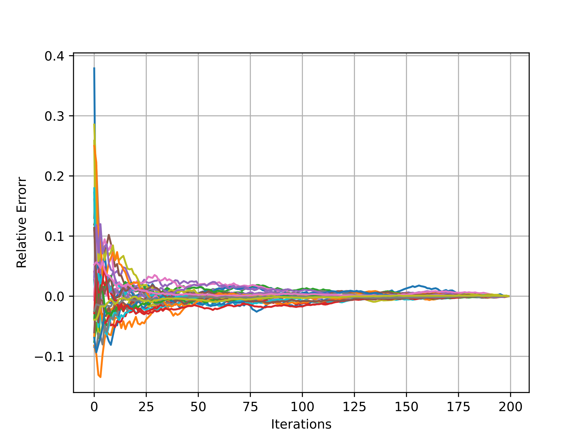
(a) ResNet18

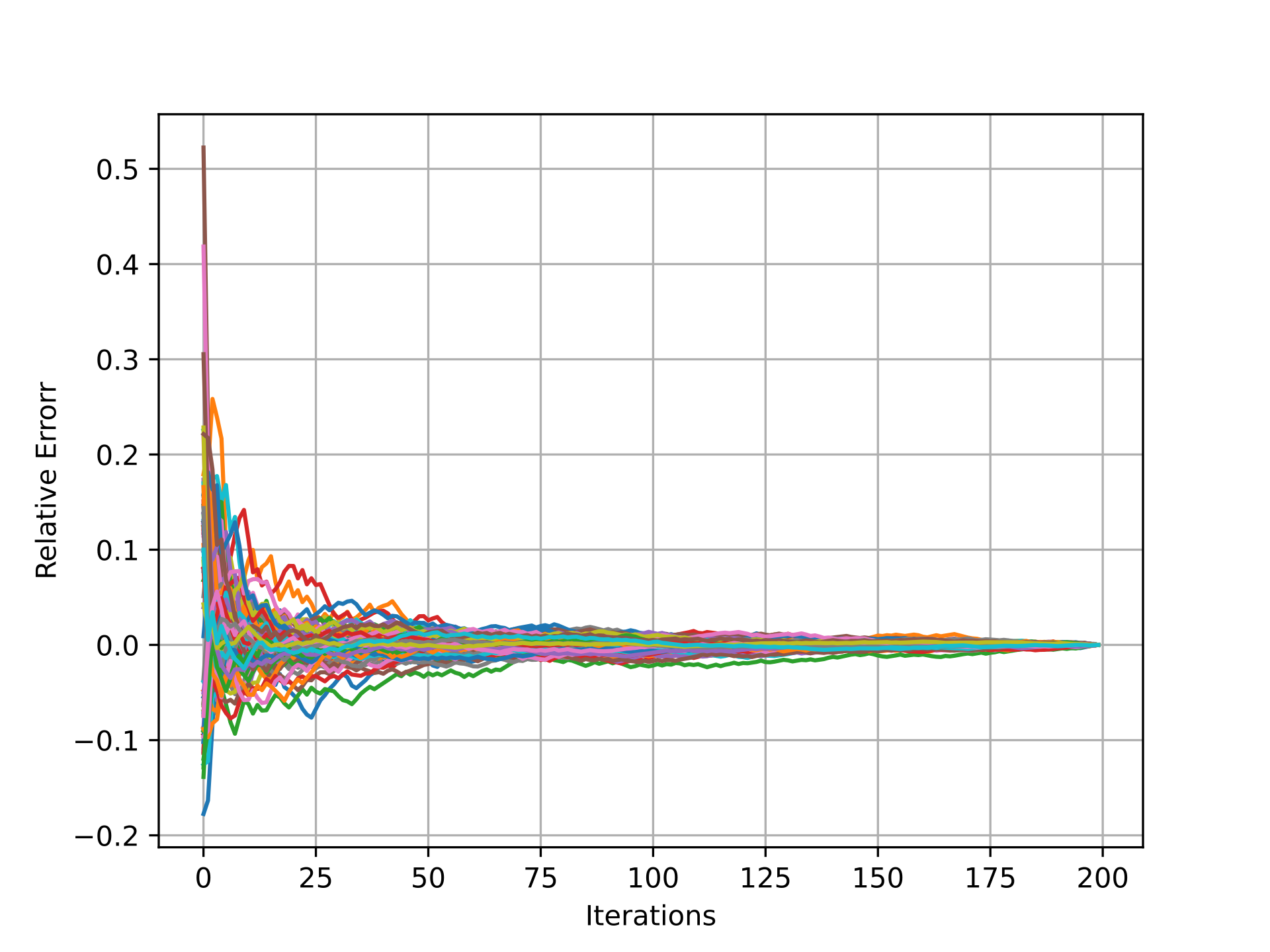
(b) ResNet50

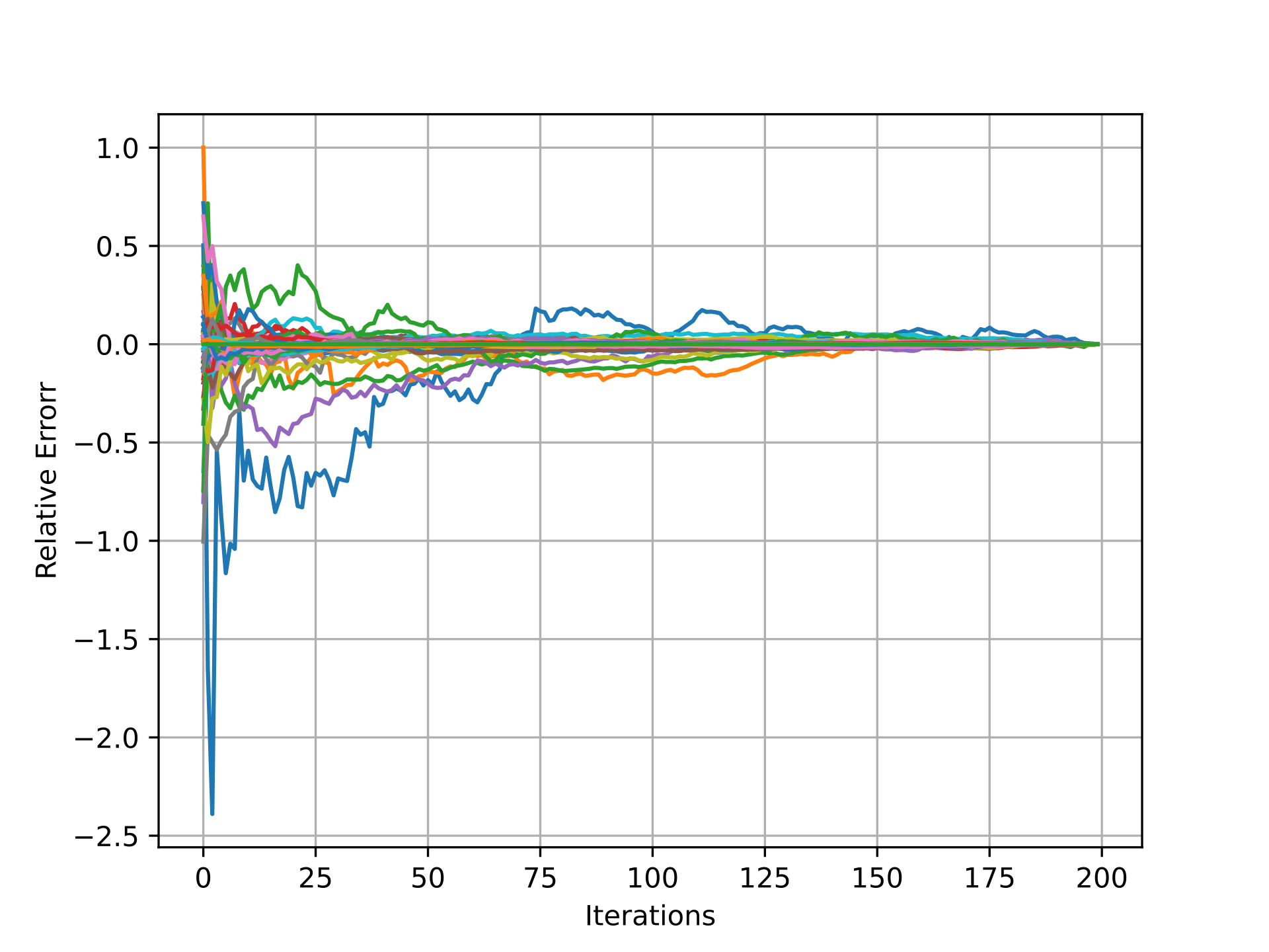
(c) MobileNetV2

Figure 7: Convergence of Label-Free Hessian, the x-axis represents the iteration number and the y-axis represents the relative error. Each color represents the converges of the algorithm for a specific activation tensor along the network.

Appendix D Mixed Precision Formulation

We formulate the mixed precision search problem to obtain a bit-width assignment for each weights quantizer under the desired memory restrictions. Let $m$ be the number of weights quantizers and $\mathcal{B}$ the set of bit-width candidates to choose from. We formulate a problem where we search for a bit-width vector $\bm{b}\in\mathcal{B}^{m}$ that minimizes knowledge distillation-based loss [7] between the floating point and the quantized models. In addition, as mentioned in Section 4.2, we define a constraint on the quantized model’s weights memory which is given by:

$$\Psi_{W}\left(\bm{b}\right)=\sum_{i\in N_{W}}\mathrm{size}\left(\mathbf{W}_{i}\right)\cdot\bm{b}_{i},$$ (18)

where $N_{W}$ is set of indices for the weight quantizers, $\bm{b}\in\mathcal{B}^{m}$ is a vector of possible bit-widths for each quantizer and $\Psi_{W}\left(\bm{b}\right)$ is the weights memory. Then, we define the general mixed precision optimization problem as follows:

$$\min\limits_{\bm{b}\in\mathcal{B}^{m}} L\left(\bm{b}\right)$$ (19)

s.t. $$\Psi_{W}\left(\bm{b}\right)\leq\psi_{W},$$

where $L$ is the objective function inspired by [7] and  $\psi_{W}$ is the target weights memory.

Following recent publications [24, 48], we assume that a layer has an independent effect on the quantization, that is, we consider the sum of each quantizer’s individual relative error as our minimization objective loss. This enables us to use an Integer Linear Programming solver to solve the mixed precision problem.

Getting an approximated solution to this problem can be achieved using any known ILP algorithm. The solution should yield a bit-width configuration that provides any configurable quantizer with a chosen bit-width for quantization.

References

- [1] Haim Avron and Sivan Toledo. Randomized algorithms for estimating the trace of an implicit symmetric positive semi-definite matrix. Journal of the ACM (JACM), 58(2):1–34, 2011.
- [2] Ron Banner, Itay Hubara, Elad Hoffer, and Daniel Soudry. Scalable methods for 8-bit training of neural networks. Advances in Neural Information Processing Systems, 31, 2018.
- [3] Ron Banner, Yury Nahshan, Elad Hoffer, and Daniel Soudry. Post-training 4-bit quantization of convolution networks for rapid-deployment. arXiv preprint arXiv:1810.05723, 2018.
- [4] Ron Banner, Yury Nahshan, Elad Hoffer, and Daniel Soudry. ACIQ: Analytical clipping for integer quantization of neural networks. In Proceedings of the International Conference on Learning Representations, 2019.
- [5] Han Cai, Chuang Gan, Tianzhe Wang, Zhekai Zhang, and Song Han. Once-for-all: Train one network and specialize it for efficient deployment. In Proceedings of the International Conference on Learning Representations, 2019.
- [6] Han Cai, Ligeng Zhu, and Song Han. Proxylessnas: Direct neural architecture search on target task and hardware. In Proceedings of the International Conference on Learning Representations, 2018.
- [7] Yaohui Cai, Zhewei Yao, Zhen Dong, Amir Gholami, Michael W. Mahoney, and Kurt Keutzer. ZeroQ: A novel zero shot quantization framework. In Proceedings of the IEEE/CVF Conference on Computer Vision and Pattern Recognition, pages 13169–13178, 2020.
- [8] Liang-Chieh Chen, Yukun Zhu, George Papandreou, Florian Schroff, and Hartwig Adam. Encoder-decoder with atrous separable convolution for semantic image segmentation. In Proceedings of the European Conference on Computer Vision (ECCV), pages 801–818, 2018.
- [9] Jia Deng, Wei Dong, Richard Socher, Li-Jia Li, Kai Li, and Li Fei-Fei. Imagenet: A large-scale hierarchical image database. In Proceedings of the IEEE/CVF Conference on Computer Vision and Pattern Recognition, pages 248–255, 2009.
- [10] Xin Dong, Shangyu Chen, and Sinno Pan. Learning to prune deep neural networks via layer-wise optimal brain surgeon. Advances in Neural Information Processing Systems, 30, 2017.
- [11] Zhen Dong, Zhewei Yao, Daiyaan Arfeen, Amir Gholami, Michael W Mahoney, and Kurt Keutzer. Hawq-v2: Hessian aware trace-weighted quantization of neural networks. In Advances in Neural Information Processing Systems, pages 18518–18529, 2020.
- [12] Zhen Dong, Zhewei Yao, Amir Gholami, Michael W Mahoney, and Kurt Keutzer. HAWQ: Hessian aware quantization of neural networks with mixed-precision. In Proceedings of the IEEE/CVF International Conference on Computer Vision, pages 293–302, 2019.
- [13] Steven K Esser, Jeffrey L McKinstry, Deepika Bablani, Rathinakumar Appuswamy, and Dharmendra S Modha. Learned step size quantization. In Proceedings of the International Conference on Learning Representations, 2020.
- [14] Pierre Foret, Ariel Kleiner, Hossein Mobahi, and Behnam Neyshabur. Sharpness-aware minimization for efficiently improving generalization. In Proceedings of the International Conference on Learning Representations, 2021.
- [15] Amir Gholami, Sehoon Kim, Zhen Dong, Zhewei Yao, Michael W Mahoney, and Kurt Keutzer. A survey of quantization methods for efficient neural network inference. arXiv preprint arXiv:2103.13630, 2021.
- [16] Amir Gholami, Kiseok Kwon, Bichen Wu, Zizheng Tai, Xiangyu Yue, Peter Jin, Sicheng Zhao, and Kurt Keutzer. Squeezenext: Hardware-aware neural network design. In Proceedings of the IEEE/CVF Conference on Computer Vision and Pattern Recognition, pages 1638–1647, 2018.
- [17] Suyog Gupta, Ankur Agrawal, Kailash Gopalakrishnan, and Pritish Narayanan. Deep learning with limited numerical precision. In International Conference on Machine Learning, pages 1737–1746. PMLR, 2015.
- [18] Hai Victor Habi, Roy H Jennings, and Arnon Netzer. Hmq: Hardware friendly mixed precision quantization block for cnns. In Proceedings of the European Conference on Computer Vision (ECCV), pages 448–463, 2020.
- [19] Hai Victor Habi, Reuven Peretz, Elad Cohen, Lior Dikstein, Oranit Dror, Idit Diamant, Roy H Jennings, and Arnon Netzer. HPTQ: Hardware-friendly post training quantization. arXiv preprint arXiv:2109.09113, 2021.
- [20] Babak Hassibi and David Stork. Second order derivatives for network pruning: Optimal brain surgeon. Advances in Neural Information Processing Systems, 5, 1992.
- [21] Yihui He, Ji Lin, Zhijian Liu, Hanrui Wang, Li-Jia Li, and Song Han. Amc: Automl for model compression and acceleration on mobile devices. In Proceedings of the European Conference on Computer Vision (ECCV), pages 784–800, 2018.
- [22] Geoffrey Hinton, Oriol Vinyals, and Jeff Dean. Distilling the knowledge in a neural network. arXiv preprint arXiv:1503.02531, 2015.
- [23] Zehao Huang and Naiyan Wang. Data-driven sparse structure selection for deep neural networks. In Proceedings of the European Conference on Computer Vision (ECCV), pages 304–320, 2018.
- [24] Itay Hubara, Yury Nahshan, Yair Hanani, Ron Banner, and Daniel Soudry. Accurate post training quantization with small calibration sets. In International Conference on Machine Learning, pages 4466–4475. PMLR, 2021.
- [25] Itay Hubara, Yury Nahshan, Yair Hanani, Ron Banner, and Daniel Soudry. Improving post training neural quantization: Layer-wise calibration and integer programming. In Proceedings of the International Conference on Learning Representations, 2021.
- [26] Benoit Jacob, Skirmantas Kligys, Bo Chen, Menglong Zhu, Matthew Tang, Andrew Howard, Hartwig Adam, and Dmitry Kalenichenko. Quantization and training of neural networks for efficient integer-arithmetic-only inference. In Proceedings of the IEEE/CVF Conference on Computer Vision and Pattern Recognition, pages 2704–2713, 2018.
- [27] Yongkweon Jeon, Chungman Lee, and Ho-young Kim. Genie: Show me the data for quantization. arXiv preprint arXiv:2212.04780, 2022.
- [28] Jangho Kim, Yash Bhalgat, Jinwon Lee, Chirag Patel, and Nojun Kwak. QKD: Quantization-aware knowledge distillation. arXiv preprint arXiv:1911.12491, 2019.
- [29] Jangho Kim, KiYoon Yoo, and Nojun Kwak. Position-based scaled gradient for model quantization and pruning. Advances in Neural Information Processing Systems, 33:20415–20426, 2020.
- [30] Yuhang Li, Ruihao Gong, Xu Tan, Yang Yang, Peng Hu, Qi Zhang, Fengwei Yu, Wei Wang, and Shi Gu. BRECQ: Pushing the limit of post-training quantization by block reconstruction. In Proceedings of the International Conference on Learning Representations, 2021.
- [31] Tsung-Yi Lin, Priya Goyal, Ross Girshick, Kaiming He, and Piotr Dollár. Focal loss for dense object detection. In Proceedings of the IEEE/CVF International Conference on Computer Vision, pages 2980–2988, 2017.
- [32] Liyuan Liu, Haoming Jiang, Pengcheng He, Weizhu Chen, Xiaodong Liu, Jianfeng Gao, and Jiawei Han. On the variance of the adaptive learning rate and beyond. In Proceedings of the International Conference on Learning Representations, 2019.
- [33] TorchVision maintainers and contributors. TorchVision: PyTorch’s Computer Vision library, Nov. 2016.
- [34] Sachin Mehta and Mohammad Rastegari. Mobilevit: Light-weight, general-purpose, and mobile-friendly vision transformer. In Proceedings of the International Conference on Learning Representations, 2021.
- [35] Asit Mishra and Debbie Marr. Apprentice: Using knowledge distillation techniques to improve low-precision network accuracy. In International Conference on Machine Learning. PMLR, 2018.
- [36] Markus Nagel, Rana Ali Amjad, Mart Van Baalen, Christos Louizos, and Tijmen Blankevoort. Up or down? adaptive rounding for post-training quantization. In International Conference on Machine Learning, pages 7197–7206. PMLR, 2020.
- [37] Markus Nagel, Mart van Baalen, Tijmen Blankevoort, and Max Welling. Data-free quantization through weight equalization and bias correction. In Proceedings of the IEEE/CVF International Conference on Computer Vision, pages 1325–1334, 2019.
- [38] Markus Nagel, Marios Fournarakis, Yelysei Bondarenko, and Tijmen Blankevoort. Overcoming oscillations in quantization-aware training. arXiv preprint arXiv:2203.11086, 2022.
- [39] Yury Nahshan, Brian Chmiel, Chaim Baskin, Evgenii Zheltonozhskii, Ron Banner, Alex M Bronstein, and Avi Mendelson. Loss aware post-training quantization. Machine Learning, 110(11):3245–3262, 2021.
- [40] Hai Victor Habi Ofir Gordon. EPTQ. https://github.com/ssi-research/eptq, 2023.
- [41] Antonio Polino, Razvan Pascanu, and Dan Alistarh. Model compression via distillation and quantization. In Proceedings of the International Conference on Learning Representations, 2018.
- [42] Liqun Qi, Shenglong Hu, Xinzhen Zhang, and Yannan Chen. Tensor norm, cubic power and gelfand limit. arXiv preprint arXiv:1909.10942, 2019.
- [43] Sheng Shen, Zhen Dong, Jiayu Ye, Linjian Ma, Zhewei Yao, Amir Gholami, Michael W Mahoney, and Kurt Keutzer. Q-bert: Hessian based ultra low precision quantization of bert. In Proceedings of the AAAI Conference on Artificial Intelligence, volume 34, pages 8815–8821, 2020.
- [44] Hugo Touvron, Matthieu Cord, Matthijs Douze, Francisco Massa, Alexandre Sablayrolles, and Hervé Jégou. Training data-efficient image transformers & distillation through attention. In International Conference on Machine Learning, pages 10347–10357. PMLR, 2021.
- [45] Xiuying Wei, Ruihao Gong, Yuhang Li, Xianglong Liu, and Fengwei Yu. QDrop: Randomly dropping quantization for extremely low-bit post-training quantization. In Proceedings of the International Conference on Learning Representations, 2021.
- [46] Ross Wightman. Pytorch image models. https://github.com/rwightman/pytorch-image-models, 2019.
- [47] Hongyi Yao, Pu Li, Jian Cao, Xiangcheng Liu, Chenying Xie, and Bingzhang Wang. RAPQ: Rescuing accuracy for power-of-two low-bit post-training quantization. arXiv preprint arXiv:2204.12322, 2022.
- [48] Zhewei Yao, Zhen Dong, Zhangcheng Zheng, Amir Gholami, Jiali Yu, Eric Tan, Leyuan Wang, Qijing Huang, Yida Wang, Michael Mahoney, et al. Hawq-v3: Dyadic neural network quantization. In International Conference on Machine Learning, pages 11875–11886. PMLR, 2021.
- [49] Zhewei Yao, Amir Gholami, Kurt Keutzer, and Michael W Mahoney. Pyhessian: Neural networks through the lens of the hessian. In IEEE International Conference on Big Data, pages 581–590, 2020.
- [50] Shixing Yu, Zhewei Yao, Amir Gholami, Zhen Dong, Sehoon Kim, Michael W Mahoney, and Kurt Keutzer. Hessian-aware pruning and optimal neural implant. In Proceedings of the IEEE/CVF Winter Conference on Applications of Computer Vision, pages 3880–3891, 2022.