Enhancing motion trajectory segmentation of rigid bodies
using a novel screw-based trajectory-shape representation
Abstract
Trajectory segmentation refers to dividing a trajectory into meaningful consecutive sub-trajectories. This paper focuses on trajectory segmentation for 3D rigid-body motions. Most segmentation approaches in the literature represent the body’s trajectory as a point trajectory, considering only its translation and neglecting its rotation. We propose a novel trajectory representation for rigid-body motions that incorporates both translation and rotation, and additionally exhibits several invariant properties. This representation consists of a geometric progress rate and a third-order trajectory-shape descriptor. Concepts from screw theory were used to make this representation time-invariant and also invariant to the choice of body reference point. This new representation is validated for a self-supervised segmentation approach, both in simulation and using real recordings of human-demonstrated pouring motions. The results show a more robust detection of consecutive sub-motions with distinct features and a more consistent segmentation compared to conventional representations. We believe that other existing segmentation methods may benefit from using this trajectory representation to improve their invariance.
I INTRODUCTION
Trajectory segmentation aims to divide a trajectory into consecutive sub-trajectories that have a specific meaning for the considered application. It is a valuable tool to reduce the dimensionality of trajectories, thereby improving the efficiency and reliability of trajectory recognition and learning algorithms. Trajectory segmentation has found applications in various research fields, including monitoring urban traffic [1], tracking changes in animal behavior [2], analyzing robot-assisted minimally invasive surgical procedures [3], and learning motion primitives for robots from human-demonstrated object manipulation tasks [4, 5, 6, 7].
In the literature, three types of segmentation approaches can be distinguished: supervised segmentation, unsupervised segmentation, and self-supervised segmentation.
Supervised segmentation algorithms rely on prior expert knowledge, such as a predefined library of template segments, such as in [8], or a set of predefined segmentation criteria. The approaches in [1, 9] segment trajectories based on criteria that assess the homogeneity of movement profiles, including the location, speed and heading of the object.
Unsupervised segmentation algorithms do not rely on prior expert knowledge. These approaches are typically event-based, searching for discrete segmentation points along the trajectory. The approach in [5] identifies segmentation points by fitting a Gaussian Mixture Model to the trajectory data and identifying regions of overlap between the confidence ellipsoids of consecutive Gaussians. Another approach involves extracting segmentation points from local extrema in curvature and torsion along the trajectory, such as in [6].
Self-supervised segmentation can be viewed as a supervised approach in which the segmentation criteria are learned from the data rather than being predetermined by expert knowledge. The segmentation approach in [10] detects transitions in movement profiles and labels them as ‘features’. Similar features are then clustered together, and subsequently, the trajectory is segmented into a sequence of cluster labels. The approach in [7] initially segments trajectories in an unsupervised way. It then learns a library of motion primitives from the segmented data, which is subsequently used to improve the initial segmentation accuracy.
The literature on trajectory segmentation has two main shortcomings. The first shortcoming is that the object is typically approximated as a moving point, considering only the translational motion while neglecting the rotational motion. Hence, not all trajectory information is taken into account.
The second shortcoming is that supervised and self-supervised segmentation approaches based on template matching typically are dependent on the motion profile of the trajectory and the choice of references. These references include both the coordinate frame in which the trajectory coordinates are expressed and the reference point on the body being tracked. This dependency limits the approach’s capability to generalize across different setups.
The main objective of this work is to enhance template-based approaches in supervised and self-supervised trajectory segmentation by incorporating invariance with respect to time, coordinate frame, and body reference point.
Our approach consists of first reparameterizing the trajectory to achieve time-invariance, i.e. invariance to changes in motion profile. This is achieved by defining a novel geometric progress rate using Screw Theory, inspired by [11]. The progress rate combines both rotation and translation, while also being invariant to the chosen body reference point. The defined progress rate is regularized to better cope with pure translations compared to [11]. After reparameterization, the trajectory is represented using a novel trajectory-shape descriptor based on first-order kinematics of the trajectory. Finally, invariance to changes in the coordinate frame is achieved by performing a spatial alignment before matching the trajectory descriptor with template segments in the library. The latter template segments are also represented using the same trajectory-shape descriptor.
The contribution of this work is (1) the introduction of a novel screw-based geometric progress rate for rigid-body trajectories, and (2) a novel trajectory-shape descriptor. These concepts were applied in a self-supervised segmentation approach using simulations and real recordings of human-demonstrated pouring motions. The results show that more consistent segmentation results can be achieved by using an invariant trajectory descriptor compared to conventional descriptors that are not invariant to changes in execution speed, coordinate frame, and reference point.
The outline of the paper is as follows. Section II reviews essential background on rigid-body trajectories and screw theory. Section III introduces the novel screw-based geometric progress rate and trajectory-shape descriptor for rigid-body trajectories. Section IV explains the implementation of these novel concepts in a self-supervised segmentation approach. Section V explains the validation of the segmentation approach using simulations and real recordings of human-demonstrated pouring motions. Section VI concludes with a discussion and suggests future work.
II PRELIMINARIES
The displacement of a rigid body in 3D space is commonly represented by attaching a body frame to the rigid body and expressing the position and orientation of this frame with respect to a fixed world frame. The position coordinates represent the relative position of the origin of the body frame with respect to the origin of the world frame. The rotation matrix , which is part of the Special Orthogonal group SO(3), represents the relative orientation of the body frame with respect to the world frame111Note that other possibilities exist for representing the orientation such as the quaternion or the axis-angle representation.. The position and orientation of the rigid body can be combined into the homogeneous transformation matrix , which is part of the Special Euclidean group . The homogeneous transformation matrix as a function of time represents a temporal rigid-body trajectory.
The first-order kinematics of the rigid-body trajectory are commonly represented by a 6D twist consisting of two 3D vectors: a rotational velocity vector and a linear velocity vector . Based on the coordinate frame in which these velocities are expressed and based on the reference point for the linear velocity , three twists are commonly defined in the literature [12, 13], i.e. the pose twist, spatial twist, and body twist. A twist is considered left- or right-invariant when it is invariant to changes of the world or body frame, respectively. The body twist is left-invariant, the spatial twist is right-invariant, and the pose twist is neither left- nor right-invariant.
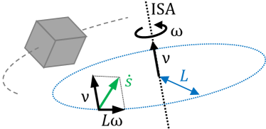
In rigid-body kinematics, the Mozzi-Chasles’ theorem [14, 15] states that a rigid-body velocity can always be represented as a rotation about an axis in space and a translation parallel to this axis, referred to as the Instantaneous Screw Axis (ISA). The direction of the ISA is uniquely defined by the direction of the rotational velocity , while the location of the ISA is defined by any point on the ISA. A unique choice is to take the point on the ISA that lies closest to the reference point for the linear velocity . This point’s position vector as well as the translational velocity parallel to the ISA, , are calculated from the twist components and :
| (1) |
When the pose twist is chosen, the coordinates of and are in the world frame, while is the position vector from the body frame’s origin to the closest point on the ISA.
The magnitudes of the rotational and translational velocities and are closely related to the ‘SE(3) invariants’ in [16] and it has been shown that they are both left- and right-invariant, also referred to as bi-invariant.
III SCREW-BASED TRAJECTORY REPRESENTATION
This section introduces a novel screw-based geometric progress rate for defining the progress over a trajectory, independent of time. Next, a new invariant trajectory-shape descriptor is introduced for rigid-body trajectories, which is both time-invariant and invariant to the choice of the reference point on the body. Invariance to changes in coordinate frame is obtained by proposing a spatial alignment algorithm.
III-A Screw-based geometric progress rate
To obtain a time-invariant representation of the trajectory, a geometric progress rate has to be defined first. We propose to combine the magnitude of the rotational velocity and the translational velocity parallel to the ISA:
| (2) |
where is a weighting factor with units [m]. The progress rate [m/s] can be interpreted as the magnitude of the linear velocity of any point on the body, at a distance from the ISA (see Fig. 1). The progress parameter [m] is then found as the integral of the progress rate over time, and can be considered as a scalar value signifying the geometric progress in translation and rotation over the trajectory.
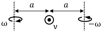
Since and are bi-invariant properties of the trajectory, as mentioned in Section II, the resulting geometric progress rate is also bi-invariant. However, it is important to clarify that the proposed progress rate does not comply with the conditions for being a bi-invariant metric on [17]. For example, consider a serial kinematic chain of two twist motions and generating a resulting motion . Then, the triangle inequality (a necessary condition for being a metric) does not hold for all cases on . Consider the example of a pure translation . This translation can be generated by a couple of rotations with magnitude , where is half the distance between the two rotation axes, as shown in Fig. 2.
Since the sum of the progress rates of these rotations equals:
| (3) |
it can be concluded that , if . Since is a predefined weighting factor and can take any value in (because can always be decreased by increasing while still resulting in the same ), there is no choice for for which the triangle inequality holds for each value of .
III-B Regularized geometric progress rate
The calculation of using (1) is degenerate for pure translations, i.e. when . Because of this, approaching a pure translation can result in approaching infinity:
| (4) |
To ensure that the calculated translational velocity of the rigid body and corresponding progress rate remain well-defined in these degenerate cases, a regularized translational velocity is introduced, such that:
| (5) |
where is a regularized version of , defined as follows:
| (6) |
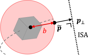
In other words, a sphere with radius is defined with the origin of the body frame as its center, so that when the position is outside of the sphere, it will be projected onto the sphere’s surface. This is also visualized in Fig. 3.
The regularization in (6) has two important properties. First, the profile of remains continuous over the threshold where , since:
| (7) |
Second, the regularization is independent of the execution speed of the motion, since is a geometric property.
In the Appendix, it is shown that choosing ensures that the triangle inequality holds within the bi-invariant region , for the example discussed in Section III-A. As a result, we propose to choose , since this results in the largest region of bi-invariance of the progress rate without violating the triangle inequality.
Remark that when , the regularized translational velocity becomes dependent on the location of the body reference point and hence loses its bi-invariant property. This is not a big problem, since the object is dominantly translating in that case. Hence, the sensitivity of the velocity to the location of the body reference point remains limited.
Algorithm 1 contains pseudocode to calculate the regularized progress rate assuming .
III-C Reparameterization to geometric domain
The temporal rigid-body trajectory can now be reparameterized to a geometric trajectory using the geometric progress rate defined in (5). As a result, the execution speed will be separated from the geometric path of the trajectory. Such a geometric trajectory is also referred to as a unit-speed trajectory, since the geometric derivative of the progress along this trajectory is equal to one:
| (8) |
In practice, for discrete measurement data, this reparameterization is performed in three steps. Firstly, the temporal pose twist is calculated from the temporal pose trajectory by numerical differentiation with the matrix logarithm operator [12]. Secondly, the progress rate is determined using Algorithm 1. The progress along the discrete trajectory is then found by a cumulative sum on . Thirdly, the trajectory is reparameterized from time to progress with fixed progress step using Screw Linear Interpolation [18].
III-D Screw-based trajectory-shape descriptor
This subsection introduces a screw-based trajectory-shape descriptor based on the rotational and translational velocities and along the reparameterized trajectory. These velocities can be calculated similarly to the calculation of and , but now starting from the reparameterized trajectory instead of . Afterwards, a normalization step is included to ensure that property (8) holds.
The proposed trajectory-shape descriptor at a given trajectory sample is of third order, and consists of the rotational and translational velocities at subsequent samples, centered at the sample point , and stacked into a matrix :
| (9) |
Since the velocities in (9) have their coordinates expressed with respect to some coordinate frame, a relative rotation alignment is needed before two local trajectory-shape descriptors can be compared. Similarly to the rotation alignment proposed in [19], shape descriptor can be aligned with in three steps:
-
1.
Obtain the singular value decomposition of the relative matrix .
-
2.
Calculate the rotation matrix , while ensuring that by changing the sign of the third column of when .
-
3.
Align with by left-multiplying with .
The difference in local trajectory-shape of two descriptors and is then defined as the Frobenius norm of the difference between the descriptors after alignment:
| (10) |
The difference is a value with units [m], measuring the difference in local change of the trajectory shape.
IV APPLICATION TO SEGMENTATION
This section applies the proposed screw-based progress rate and trajectory-shape descriptor to a trajectory segmentation approach. Envisioned towards incremental learning applications, a self-supervised segmentation approach based on incremental clustering was devised. This segmentation approach consists of two phases: an offline learning phase where a library of trajectory-shape primitives is learned, and a trajectory segmentation phase.
Offline template learning: Trajectory-shape primitives are learned by an incremental clustering approach, where the mean of each cluster represents a learned primitive. The clustering approach consists of four steps:
1) Initialization: Use the first sample point to generate the first cluster with mean and a chosen initial guess for its standard deviation .
2) Cluster growing: Given a sample point with corresponding trajectory-shape descriptor , calculate the difference between the descriptor and the mean of every learned cluster. Afterwards, add the sample point to the cluster with the smallest difference in trajectory-shape, if this difference is smaller than three times its standard deviation , and update the mean and standard deviation of the cluster accordingly. If no such cluster exists, create a new cluster with mean and initial standard deviation .
3) Cluster parameter update: After all the available data is clustered, update the value for based on the mean of the standard deviations of all the learned clusters : , with a tuning parameter related to the process noise of the clusters. Iterate steps 1 to 3 until converges to a steady value.
4) Outlier removal: After convergence, remove sparse clusters that do not represent at least of the data, with being a chosen value.
Trajectory segmentation phase: Each sample point gets associated with a learned primitive (using a 1-Nearest-Neighbor classifier) as long as the difference in trajectory-shape is smaller than of the respective cluster. Otherwise, the sample point is labeled as ‘non-classified’. Afterwards, segments are formed by grouping consecutive sample points along the trajectory that were associated with the same trajectory-shape primitive.
V EXPERIMENTS
A key property of the proposed trajectory representation is its invariance to time and the choice of body reference point. The main aim of the experiments is to demonstrate the advantages of these invariant properties for trajectory segmentation. This is done both in simulation and using real recordings of human-demonstrated pouring motions.
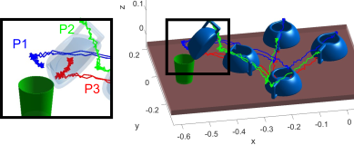
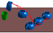
The simulated trajectories represent temporal rigid-body trajectories of pouring motions performed with two types of objects: a teakettle and a bottle. The strategy of the pouring motion consists of a sequence of six intuitive sub-motions, also visualized in Fig. 4:
-
•
slide+ : the object is slid across the table from its initial position to a fixed location on the table
-
•
lift+ : the object is lifted and reoriented so that the spout is directed towards the glass
-
•
tilt+ : the object is tilted to pour the liquid
-
•
tilt- : the object’s tilt is undone
-
•
lift- : the object is placed back on the table
-
•
slide- : the object is slid back
We aim to robustly segment the pouring motion into these sub-motions. To simulate sensor noise, white noise with a standard deviation of 2 and 1 mm were added to the object’s orientation and reference point’s location, respectively.
To study robustness to changes in the body reference point, each of the three trajectories was simulated with a different reference point: the first was near the spout (P1), the second near the handle (P2), and the third near the center of mass (P3). Fig. 4 on the left illustrates that, when rotation of the object is involved, the different reference points result in significantly different point trajectories.
The generalization capability is tested by applying the primitives that were learned for the kettle motion to another object. The object was chosen to be a bottle of which the reference point was chosen in the center of its opening.
The proposed approach is compared to other methods based on the literature, shown in Table I. Method does not transform the object’s trajectory to a geometric domain. Methods and neglect information on the object’s orientation by choosing . Methods and use the arclength of the reference point’s trajectory as the geometric progress parameter, such as in [19]. Method uses the traveled angle of the moving object as the geometric progress parameter, such as in [20]. Method uses a combination of the rotational velocity and linear velocity of the reference point on the body as the progress rate, such as in [17]. Method uses a screw-based progress rate without the proposed regularization, such as in [11]. Method uses the proposed screw-based geometric progress rate.
| method | progress-type | [cm] | ||||
|---|---|---|---|---|---|---|
| A | time | 0 | 0.1s | 10cm/s | 2% | |
| B | arclength | 0 | 2cm | 2cm | 5% | |
| C | arclength | 30 | 2cm | 10cm | 5% | |
| D | angle | 30 | 3° | 10cm | 5% | |
| E | combined | 30 | 2cm | 10cm | 5% | |
| F | screw-based | 30 | 2cm | 10cm | 5% | |
| G | screw-based | 30 | 2cm | 10cm | 5% |
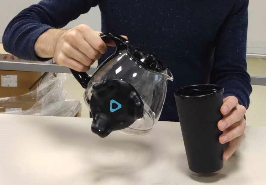
To validate that the proposed method works in practice, it was tested on recordings of real pouring motions. These motions were recorded using an HTC VIVE motion capture system, consisting of a tracker attached to the kettle (see Fig. 5a), and two base stations. The VIVE system recorded the pose trajectories with a frequency of 60 Hz and an accuracy in the order of a few mm and a few degrees. To introduce contextual variations in the measurements, the tracker was physically attached to the kettle at two different locations, one at the side of the kettle (P1) and one near the top of the handle (P2). For each tracker location, three trials were recorded. Fig. 5b depicts the kettle’s pose trajectory for the first trial with the tracker attached to the side.
V-A Data processing
The simulated data and the recorded data were processed in the same way. The rigid-body trajectories were first preprocessed using a Kalman smoother with a constant acceleration model to deal with the effects of the measurement noise. For the methods to , the trajectories were first reparameterized as in Section III-A according to the chosen definition of the progress rate . Then, the local shape descriptor was calculated as in Section III-D. Finally, the same segmentation algorithm (Section IV) is applied for all approaches. For reproducability reasons, all software used in the experiments is made publicly available [21].
The values of the tuning parameters are reported in Table I. A good choice for depends on numerous factors, including the scale of the motion and the scale of the moving object. Given the scale of the objects and motions of interest, a value of cm seemed reasonable. The other parameters in Table I were manually tuned. For method , the parameters and have different units compared to the ones of the other methods since method does not transform the trajectories to a geometric domain before segmentation.
V-B Results
Simulated data: Fig. 6 visualizes the segmentation results of all methods for the simulated data. The ground-truth segmentation points are indicated by the vertical lines. To compare between methods, the segmented trajectories were transformed back to the time domain by re-applying the motion profile that was extracted from the trajectories. This was done by inverting the reparameterization procedure of Section III-C. The segmentation results are also evaluated quantitatively by reporting the number of detected sub-motions and consistent segments. A sub-motion was considered ‘detected’ when a corresponding segment was formed. A sub-motion was considered ‘consistently segmented’ when the corresponding segments were associated to the same trajectory-shape primitive across the three trials.
The results of the simulation are interpreted as follows. Method generated a relatively high number of segments. The segmentation is mainly based on differences in magnitude of the reference point’s velocity. The gray segments represent regions of standstill. The light and dark blue segments represent segments of low and high magnitude in velocity, respectively. Methods to generated segments based on differences in shape of the rigid-body trajectory.
For methods -, the learning of the primitives and segmentation of the trajectories was dependent on the location of the reference point on the object. Furthermore, methods - could not deal well with pure rotations of the object. Method classified these segments either as stationary or as segments with low magnitude in velocity. Methods and treated these segments as outliers. The reason for this is that during these pure rotations, the traveled arclength of the reference point remained relatively small, resulting in a small number of geometric sample points representing these pure rotations. Hence, for pure rotations, sparse clusters were created, which were seen as outliers. Following a similar reasoning, method could not deal with pure translations.
Method performed the segmentation in a reference-point invariant way, but could not deal well with pure translations, since is degenerate in this case.
The proposed method dealt well with pure translations and performed the segmentation in a reference-point invariant way. The trajectories of the kettle were consistently segmented into six segments, corresponding to the six intuitive sub-motions. More in detail, all sub-motions were detected (6/6) and all sub-motions were consistently segmented (6/6). Fig. 7 visualizes the segmented trajectories.

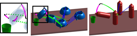
The proposed approach also succeeded to segment the simulated pouring motion performed with a bottle (with significantly different location of the reference point) using the trajectory-shape primitives learned from the trajectories of the kettle. This illustrates the capability of the approach to generalize to different objects with different geometries.
Real data: Fig. 8 visualizes the segmentation results of the proposed method for the real recorded pouring motions. To illustrate the generated segments in the geometric domain, the extra transformation back to the time domain was not performed. The same values for the tuning parameters as reported in Table I were used for this experiment.
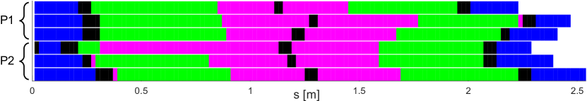
Three primitives were learned from the real data. The corresponding values of the mean trajectory-shape descriptor of the three clusters are reported in Table II. The learned primitives represent 1D motions, since for each primitive, the three columns are almost identical. The first primitive represents a 1D translation (slide). The second primitive represents a rotation with a non-zero pitch (lift). The third primitive represents a pure rotation (tilt). The segmentation approach created segments conform the six intuitive sub-motions, apart from some short segments near transition regions. These short segments can be avoided by implementing a postprocessing step or a more advanced segmentation algorithm from the literature, which is part of future work.
| -0.02 | -0.02 | -0.02 | 0.97 | 0.97 | 0.97 | 1.00 | 1.00 | 1.00 | |
| -0.01 | -0.01 | -0.01 | -0.03 | -0.01 | -0.02 | 0.01 | -0.00 | -0.01 | |
| 0.12 | 0.11 | 0.11 | 0.02 | 0.01 | 0.01 | 0.03 | -0.00 | -0.03 | |
| 0.99 | 0.99 | 0.99 | 0.26 | 0.26 | 0.26 | 0.06 | 0.06 | 0.06 | |
| 0.01 | 0.01 | 0.01 | -0.00 | 0.01 | 0.01 | 0.00 | 0.00 | -0.00 | |
| -0.11 | -0.11 | -0.11 | -0.01 | -0.02 | -0.01 | 0.00 | 0.00 | -0.00 | |
VI DISCUSSION AND CONCLUSION
The objective of this work was to enhance template-based trajectory segmentation approaches by incorporating invariance. Time-invariance was achieved by reparameterizing the trajectory using a novel geometric progress parameter. By considering the translation along the screw axis, the progress parameter was made invariant to the choice of body reference point. Based on the reparameterized trajectory, a screw-based trajectory-shape descriptor was proposed to characterize the local geometry of the trajectory.
For the devised self-supervised segmentation scheme, the results showed a more robust detection of consecutive sub-motions with distinct features and a more consistent segmentation thanks to the invariant properties of the screw-based progress parameter and the trajectory-shape descriptor.
The proposed approach also has a more practical advantage. Due to the invariance, the formation of the segments becomes invariant to changes in sensor setup (i.e. changes in the location and angle of the camera, changes in the location of markers or trackers on the object, etc.). Therefore, sensor calibration efforts can be reduced.
Future work is to examine the benefits of the invariant segmentation approach for other types of object manipulation tasks and to verify the extent to which other segmentation methods may benefit from the invariant approach.
APPENDIX
This appendix shows that the triangle inequality property in Section III-B is always satisfied for the regularized progress rate if equals in (6).
Consider again the case of a couple of rotations generating a translation as explained in Section III-B. Additionally consider that the rotation axes of the couple are symmetrically positioned w.r.t. the reference point, such that . Equation (3) then remains valid under the proposed regularization action when . From (3), it was derived that the triangle inequality holds when . Hence, given that and , then is always satisfied when .
References
- [1] S. Dodge, R. Weibel, and E. Forootan, “Revealing the physics of movement: Comparing the similarity of movement characteristics of different types of moving objects,” Computers, Environment and Urban Systems, vol. 33, no. 6, pp. 419–434, 2009.
- [2] M. Teimouri, U. G. Indahl, H. Sickel, and H. Tveite, “Deriving animal movement behaviors using movement parameters extracted from location data,” ISPRS International Journal of Geo-Information, vol. 7, no. 2, 2018.
- [3] S. Krishnan, A. Garg, S. Patil, C. Lea, G. Hager, P. Abbeel, and K. Goldberg, “Transition state clustering: Unsupervised surgical trajectory segmentation for robot learning,” The International Journal of Robotics Research, vol. 36, no. 13-14, pp. 1595–1618, 2017.
- [4] M. Wächter and T. Asfour, “Hierarchical segmentation of manipulation actions based on object relations and motion characteristics,” in International Conference on Advanced Robotics, 2015, pp. 549–556.
- [5] S. H. Lee, I. H. Suh, S. Calinon, and R. Johansson, “Autonomous framework for segmenting robot trajectories of manipulation task,” Autonomous Robots, vol. 38, pp. 107–141, 2014.
- [6] C. Song, G. Liu, X. Zhang, X. Zang, C. Xu, and J. Zhao, “Robot complex motion learning based on unsupervised trajectory segmentation and movement primitives,” ISA Transactions, vol. 97, pp. 325–335, 2020.
- [7] D. Kulic, W. Takano, and Y. Nakamura, “Online segmentation and clustering from continuous observation of whole body motions,” IEEE Transactions on Robotics, vol. 25, no. 5, pp. 1158–1166, 2009.
- [8] F. Meier, E. Theodorou, F. Stulp, and S. Schaal, “Movement segmentation using a primitive library,” in 2011 IEEE/RSJ International Conference on Intelligent Robots and Systems, 2011, pp. 3407–3412.
- [9] M. Buchin, A. Driemel, M. J. van Kreveld, and V. S. Adinolfi, “Segmenting trajectories: A framework and algorithms using spatiotemporal criteria,” Journal of Spatial Information Science, vol. 3, pp. 33–63, 2011.
- [10] Z. Izakian, M. S. Mesgari, and R. Weibel, “A feature extraction based trajectory segmentation approach based on multiple movement parameters,” Engineering Applications of Artificial Intelligence, vol. 88, p. 103394, 2020.
- [11] J. De Schutter, “Invariant description of rigid body motion trajectories,” Journal of Mechanisms and Robotics, vol. 2, no. 1, pp. 011 004/1–9, 2010.
- [12] K. Lynch and F. Park, Modern Robotics. Cambridge University Press, 2017.
- [13] H. Bruyninckx, “Robot kinematics and dynamics,” https://u0011821.pages.gitlab.kuleuven.be/pdf/2009-HermanBruyninckx-robotics-textbook.pdf, November 2021, course notes, Department of Mechanical Engineering, KU Leuven.
- [14] M. Chasles, “Note sur les propriétés générales du système de deux corps semblables entr’eux et placés d’une manière quelconque dans l’espace; et sur le déplacement fini ou in infiniment petit d’un corps solide libre,” in Bulletin des Sciences Mathématiques, Astronomiques, Physiques et Chimiques, vol. 14, 1830, pp. 321–326.
- [15] M. Ceccarelli, “Screw axis defined by giulio mozzi in 1763 and early studies on helicoidal motion,” Mechanism and Machine Theory, vol. 35, no. 6, pp. 761–770, 2000.
- [16] G. Chirikjian, “Partial bi-invariance of se(3) metrics 1,” Journal of Computing and Information Science in Engineering, vol. 15, p. 011008, 2015.
- [17] F. C. Park, “Distance Metrics on the Rigid-Body Motions with Applications to Mechanism Design,” Journal of Mechanical Design, vol. 117, no. 1, pp. 48–54, 1995.
- [18] L. Kavan, S. Collins, J. Žára, and C. O’Sullivan, “Geometric skinning with approximate dual quaternion blending,” ACM Transactions on Graphics (TOG), vol. 27, no. 4, pp. 1–23, 2008.
- [19] Y. Guo, Y. Li, and Z. Shao, “Dsrf: A flexible trajectory descriptor for articulated human action recognition,” Pattern Recognition, vol. 76, pp. 137–148, 2018.
- [20] B. Roth, “Finding geometric invariants from time-based invariants for spherical and spatial motions,” Journal of Mechanical Design, vol. 127, no. 2, pp. 227–231, 2005.
- [21] “Self-supervised segmentation of temporal rigid body trajectories,” https://gitlab.kuleuven.be/robotgenskill/public_code/segmentation_paper_code.