Creases and cusps in growing soft matter

Abstract

The buckling of a soft elastic sample under growth or swelling has highlighted a new interest in materials science, morphogenesis, and biology or physiology. Indeed, the change of mass or volume is a common fact of any living species, and on a scale larger than the cell size, a macroscopic view can help to explain many features of common observation. Many morphologies of soft materials result from the accumulation of elastic compressive stress due to growth, and thus from the minimization of a nonlinear elastic energy. The similarity between growth and compression of a piece of rubber has revived the instability formalism of nonlinear elastic samples under compression, and in particular Biot’s instability. Here we present a modern treatment of this instability in the light of complex analysis and demonstrate the richness of possible profiles that an interface can present under buckling, even if one restricts oneself to the two spatial dimensions. Special attention is given to wrinkles, folds and cusps, a surprising observation in swelling gels or clays. The standard techniques of complex analysis, nonlinear bifurcation theory and path-independent integrals are revisited to highlight the role of physical parameters at the origin of the observed patterns below and above the Biot threshold.

I Introduction

The buckling of the outer surface of a living tissue during growth [1, 2, 3] and the corrugation of the surface of a swelling gel [4, 5, 6] are often observed in nature or in the laboratory. In the last three decades, a large number of studies have been devoted to such patterns in order to explain complex geometries in embryogenesis [7, 8, 9], botanical morphogenesis [10, 11, 12], but also in tumorogenesis [13, 14, 15] and organ pathologies (e.g. wound healing [16, 17, 18]). These shape instabilities affect thick samples that experience large volume variations in a non-isotropic manner. Obviously, in a free environment, the constant growth of a homogeneous sample does not generate stress, but if there is a constraint, such as a substrate, or if there is a material or growth inhomogeneity, then the stress is generated that changes the shape of the body. It can buckle, but only if there is enough growth. This suggests a shape change once the relative volume increase exceeds a threshold, about 2 times the original. The origin of the observed patterns at free surfaces results from the compressive stress generated by growth coupled with the hyperelastic properties of soft tissues. These tissues exhibit large deformations even at low stress values, and classical linear elasticity cannot explain the observed shapes. Focusing on the simplest case of a gel layer of constant thickness $H_{0}$ placed on a substrate, the growth process occurs mainly in the vertical direction and leads to a thickening of the layer with: $H=J_{t}H_{0}$, where $J_{t}$ is the relative growth per unit volume at a time $t$ in this simple geometry. When $J_{t}$ is increased to a critical value, the top surface begins to wrinkle. For neo-Hookean elasticity, this value $J_{B}$ of order $3.38$ can be related to the critical value found by Biot for samples under compression. Of course, this instability is common and not limited to the ideal gel layer. The threshold for wrinkling depends on the nonlinear elasticity model [19, 20], or on the initial geometry of the sample [21, 16], or possibly on the growth anisotropy [22], but the order of magnitude of this number seems quite robust.

The mechanical interpretation of a material under compression was first given by M.A. Biot in a seminal paper ”Surface instability of rubber in compression” [23]. Surface instability means that the instability is more visible at the surface of the sample, but actually occurs throughout the volume, as opposed to the Azaro-Tiller-Grenfield instability [24, 25], which results from surface diffusion. This instabilty is also different from wrinkles formed by a two-layer system where the top layer is thin and stiff and plays the role of a hard skin [26]. In this case, the surface topography can be realized in a very controlled way and is of enormous importance in industrial and biomedical applications [27]. Biot’s instability was first demonstrated for a compressed neo-Hookean hyperelastic sample with a free surface in infinite geometry. It describes a two-dimensional infinite periodic pattern that occurs above a characteristic threshold for the compression level, but when the material geometry is more complex, such as bilayers [28, 20], or when the compression results from anisotropic or inhomogeneous growth, the interface buckling is recovered experimentally, but the analysis can be less straightforward. However, if smooth surface undulations can also be considered [29], the experimental patterns quickly evolve to nonlinear mode coupling [30, 31, 32, 33, 34] and even to wrinkles, which are less understood, although they are easily and commonly observed in experiments and are also noted in the physiology of the brain cortex, for example [35].

An even more puzzling observation concerns more cusped interfaces as shown in Fig.(1) (A1) to (A6). In one dimension, a cusp is a special point of a curve where the radius of curvature vanishes (or the curvature is infinite), while a ”wrinkle” represents a more or less deep local folding of the interface. Other different interpretations of surface wrinkles concern singular points at the origin of a self-contacting interface, which of course indicates a much more singular interface deformation, see Fig. (1) (A9) and [36, 37, 38, 39, 40]. Do they result from a highly nonlinear coupling of modes occurring after the bifurcation, or do they belong to another class of solutions? In the latter case, they can appear below the Biot threshold $J_{B}$ and even inhibit the classical instability [41, 42]. More recently, the idea that there can be new families of solutions below the Biot threshold has been supported by matched asymptotic analysis [36, 37, 38, 39, 40] or by the nucleation of new solutions in more complex elasticity models and geometries [43, 20]. Some experimental evidence realized on rubber in compression or on swelling gels also seems to favor the second hypothesis [36, 37, 44]. Of course, numerical evidence is always difficult in the case of spatial singularities, but we must mention the finite element numerical investigation of [45, 46] in favor of a subcritical (or discontinuous bifurcation) before $J_{B}$ which becomes supercritical (or continuous) at $J_{B}$ with an important sensitivity of the results to the conditions imposed on the substrate. Another way to study the cusp formation experimentally and theoretically [38] is to create a localized defect in a controlled experiment, mimicking in some way experiments in viscous fluids where the defect is realized by contra-rotating cylinders [47]. It should be noted that localized singular structures easily occur in tubes but here the geometry helps the appearance of singular deformations [48, 49].

Despite the similarity that exists between compressive forcing and homogeneous growth in the neo-Hookean approach, this review article focuses on volumetric growth, which is ubiquitous in life. Most of our organs exhibit Biot’s instability, which explains our fingerprints, the convolutions of our brains, the villi and the mucosa of the intestines. All these structures appear after a certain time after fertilization in foetal life. They are present in most mammals, except for small rodents. These two observations support an interpretation in terms of morpho-elasticity: the shape of the organ is a determinant factor, as is the volumetric growth, which increases with time from $J=1$ (no growth expansion) up to critical values.

Before giving mathematical proofs concerning wrinkles, our presentation will begin with a selection of experiments (section II) and a brief introduction to the principles of nonlinear elasticity. In this field of study, positive quantities called invariants $I_{J}$ are introduced to evaluate the elastic energy density. Since they are specific to finite elasticity, they will be introduced in detail in section III. In addition, the local growth per unit volume creates an external field that does not obey physical rules and is imposed a priori inside the sample. It is not fully comparable to an externally applied compressive dead load, see Sec. IV. We first revisit the original model of Biot for neo-Hookean elasticity in the incompressibility limit and in semi-infinite geometry [50, 23], but for the threshold determination $J_{B}$ and for nonlinear buckling and wrinkling, we follow a different strategy based on variational principles. Euler-Lagrange equations derived by incremental perturbation techniques are at the origin of the periodic modes and also of $J_{B}$, the threshold. We then apply the nonlinear techniques of bifurcations, combined with complex analysis, which greatly simplifies the intermediate algebra. The results of Biot are recovered in a much simpler way and nonlinearities are treated above and below the threshold without difficulty. First, subcritical bifurcations, as indicated by [51, 52, 53], are demonstrated by nonlinear sinusoidal mode coupling. Second, wrinkles above and below the Biot threshold are analytically justified by introducing singularities either inside or above the elastic sample.

This notion can be rather abstract, but has been successfully introduced for interfacial flows such as viscous fingering [54, 55, 56, 57], for bubbles in Laplacian and Stokes flows [54, 58], for vortices [59, 60], and for diffusive growth [61, 62]. In fluids, singularities outside the physical plane are used to select the length scale of the interface patterns, but they can be physically introduced into the flow in the experimental setup, leading to a complete change of the interface shape. For example, a coin or a bubble in front of a viscous finger completely changes the shape into a dendritic one [63], and a theoretical interpretation has been given in terms of a dipole.
This idea of a dipole was taken up later [64] in fluids and in linear elastic solids. Also, when vortices are created in viscous fluids, they generate cusps at the interface [65, 66] (in the mathematical sense), which are transformed into sharp wrinkles when a weak surface tension is included [47, 67]. Following a similar strategy, we will consider singularities outside and inside the physical domain, with the aim of discovering the main physical ingredients necessary to predict the observed wrinkles.

In conclusion, the existence of wrinkles in growing soft materials benefits from many theoretical analyses carried out in the last decades on viscous flows (interfacial and vortex flows) and from treatments of singularities in elasticity based on the Noether theorem and path independent integrals, see section XII. These classical but not easy techniques are presented in the following. We limit ourselves to a very simple modeling of hyperelasticity, being convinced that, once established, it will be possible to extend the mathematics to arbitrary geometries and complex structures of soft materials. After the presentation of some experimental examples in section II and a reminder of the foundations of nonlinear or finite elasticity (sections III to VI), we focus on a variational energy method, section VII, where buckling modes are treated at the linear, (section VIII), and nonlinear, (section IX), levels. We then study the possibility of stress focusing [68] inside the material just below the interface, which can induce interfacial wrinkles, in section X. If these zones can be perfectly characterized in morphoelastic growth, (section XI), there is no clear threshold for their observation as demonstrated by the technique of path independent integrals, (section XII). Finally, we come back to the buckling of thin films of finite thickness comparable to the wavelength in section XIII.

II Selection of creases in experiments

The formation of wrinkles and creases in samples of elastomers or swelling gels has fascinated physicists for decades and probably still does. Examples of compressed elastomers are given in Fig.(1) panels $A1,A2,A4$, and all the other panels concern swelling gels in different experimental setups. In fact, the nucleation of wrinkles in materials known to be highly deformable without plasticity is quite astonishing. It contrasts with the difficulty of nucleating a fracture in a 3D brittle sample under tensile loading: in this case, an initial notch or slit must be deliberately made [69, 70]. Experimentally, it is difficult to elucidate the threshold for the appearance of these wrinkles. Indeed, the homogeneous volumetric growth of a material is equivalent to a compression, but the linear instability threshold discovered by Biot has not been precisely verified experimentally. As for wrinkles, it seems even worse, although there is a tendency to detect them above the Biot threshold. It is true that the geometry of the experimental setup has its importance on the threshold, as well as the fact that the material is attached to a solid substrate or to another elastic sample. Another important point concerns the size of the experimental setup compared to the instability wavelength and the fact that the neo-Hookean model (or any hyperelastic model) is not really adapted to swelling. The poroelastic model is more appropriate in this case [71, 36, 14]. Independently, R. Hayward and collaborators [72, 42, 53] point out in a series of articles that the bifurcation around the Biot threshold is probably subcritical, which makes a precise experimental determination difficult. However, singular profiles certainly exist, and the last panel (A9) shows the strong stress concentration that leads to the ejection of material pieces from the outer ring [73, 74] during the course of the experiment. Our main concern in the following will be the prediction of patterns around the Biot threshold or below. Nevertheless, let us recall the theory of finite elasticity with or without growth. It will be a way to introduce the main principles of application as well as the mathematical tools. A short presentation of the theory of swelling gels is also included to emphasize the difference between swelling and volumetric growth.

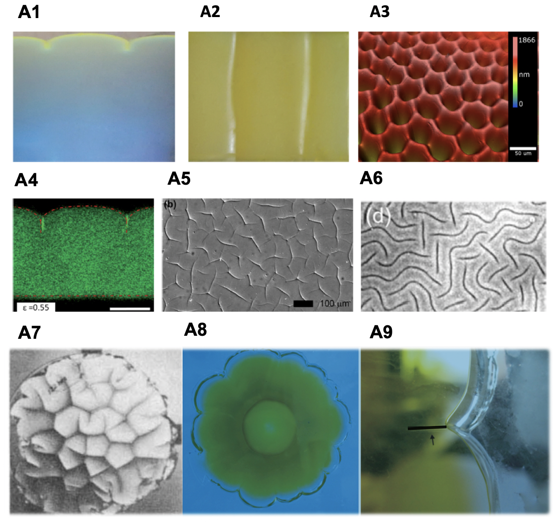
Figure 1: In (A1) and (A2), compression of a parallelepiped specimen: micrographs of a pair of wrinkles from the front and from the top view at a strain level of $45\%$, above the Biot threshold. [75]. The critical strain for wrinkling is $37.2\%$. In (A3) experimental herringbone array of a PDMS swelling gel sample, courtesy of Derek Breid [51, 52].
In (A4) Confocal microscopy for elastomer surfaces under compressive strain with an initial thickness of $23\mu$m [76]. In (A5) and (A6) two optical micrographs of wrinkle growth for a gel containing $15$ mol $\%$ NaAc, obtained by cooling, with an initial thickness of $15\mu$m [77], in (A5) from to $33.2^{\circ}C$ C to $31.7^{\circ}C$ in (A6) up to to $25^{\circ}C$.
In (A7) Creases in circular geometry: a pioneering experiment by T. Tanaka et al. on the swelling of an ionized acrylamide gel in water. In (A8) A ring of charged polyacrylamide gel (yellow) around a hard disk of neutral polyacrylamide gel (transparent) viewed from above: initial diameter: $50$ mm and imposed thickness of $1$ mm. The outer ring swells by immersion in distilled water; the swelling is highly inhomogeneous in this geometry. The inner disk acts as a constraint, and after the appearance of smooth wrinkles, wrinkles develop at the outer boundary above a certain threshold of volume variation [14]. In (A9) the same experimental setup as in (b) with a focus on a single cuspoidal point [74]. For clarity, the attached line of fracture or refolding has been underlined in black. Note that it may appear as a self-contacting interface or as a fracture in compression [38] .

III A basic introduction to nonlinear elasticity

III.1 A brief reminder of the principles of linear elasticity

Linear elasticity is limited to weak to moderate deformations corresponding to small strains, estimated by the ratio: deformation over a typical length of the deformed specimen. These deformations often occur under external loads, possibly under external fields such as temperature changes. Unlike other heuristic models, such as the Canham-Helfrich [78, 79] models for lipid membranes, elasticity requires knowledge of the initial shape of the body, which is assumed to be free of stress, and focuses on its deformation. Until recently, the goal was to explain and quantify the deformations of stiff materials: steel, wood, concrete, paper, nylon, etc., and their stiffness is usually given by the Young’s modulus $E$ in Pascals. For these materials, the value of $E$ is on the order of $10^{9}$ to $10^{12}$ Pascals, which immediately indicates that it will be very difficult to stretch a cuboid by human force. Nevertheless, the field of linear elasticity remains very active: Being closely related to geometry, any peculiarity leads to a strong interest and curiosity, such as the crumpling of paper [80, 81, 82, 83], the formation of folds [84, 85, 86], or the science of origami [87, 88]. The linearity of the relationship between displacement and load does not automatically imply that the equilibrium equations are linear, as demonstrated by the Foppl-Von Karman equation, where the Hooke formalism is applied but the deformation is extended to the third order [89]. In particular, origami and paper crumpling studies introduce geometric singularities that can be treated with linear elasticity [68], while folding involves nonlinear elasticity. The linearity of the Hooke’s law does not automatically imply simplicity of the theoretical treatment when the initial shape is complex. In fact, the formalism leads to partial differential equations, and this geometric complexity is also recovered in nonlinear elasticity. Thus, the main question is when nonlinear elasticity is required a priori.

III.2 The principles of nonlinear elasticity

Once a material is soft, even very soft, with a Young’s modulus $E$ not greater than $10^{5}$, the displacement of any point of the sample under load can be of the order of the original shape. Then, a precise description for the internal stresses and also for the geometry of the deformations are required. Not all nonlinear descriptions of the elastic energy density W are possible because they must satisfy strong mathematical properties dictated by the laws of mechanics, such as objectivity and convexity. Objectivity means that the elastic energy remains invariant under rigid rotation or translation. Convexity means that for small displacements $u$, $\delta W\sim\alpha u^{2}$ with $\alpha>0$. We consider an undeformed body with no internal stresses, where each point $M$ is represented by the capital letters $M(X,Y,Z)$ (for simplicity, Cartesian coordinates are chosen and maintained throughout the manuscript). Then there exists a vectorial mapping function $\chi$ such that relates the new coordinates of the displaced point $m$ to the coordinates of the original point such that $\vec{O}m=\vec{O}M+\vec{u}$. $\vec{u}$ is the vector displacement according to the same definition as in linear elasticity. One of the most important mathematical tools is the deformation gradient tensor which reads:

$${\bf F}=\nabla\chi\quad{\mbox{where}}\quad F_{ij}=\frac{\partial x_{i}}{\partial X_{j}}=\delta_{ij}+\frac{\partial u_{i}}{\partial X_{j}}\,.$$ (1)

The hyperelastic energy density $W$ must respect spatial isotropy (if there is no preferred direction in the structure of the body) and be invariant for any change in the coordinate system. Consequently, it must be represented by the trace or determinant of tensors constructed with ${\bf F}$. We start with the simplest invariants, the most common one being defined with the Cauchy right tensor $\bf C=\bf F^{T}\bf F$ to satisfy the objectivity requirement.

$$I_{1}=\rm{Tr}({\bf C})\quad I_{2}=\frac{1}{2}\left\{(Tr({\bf C}))^{2}-Tr({\bf C}^{2})\right\},$$ (2)

$I_{1}$ can be written as $I_{1}=F_{ij}\cdot F_{ij}$ where summation on repeated indices holds. The third invariant $I_{3}=$Det$({\bf F})$ is related to the local volume variation and must be a positive number. Homogeneous hyperelastic energy densities are basically functions of these $3$ invariants, but can also be restricted to two of them, generally $I_{1}$ and $I_{3}$ as for the neo-Hookean energy density, while the linear combination of $I_{1}$, $I_{2}$ and $I_{3}$ is called the Mooney-Rivlin model. One may wonder how to recover the weakly nonlinear energy density described by the Lamé coefficients. The simplest way is to define $\bf H=F-I$  first, and then the elastic energy density W as

$$W=\frac{1}{2}\left\{\mu_{L}(\mbox{Tr }({\bf H^{T}}\cdot{\bf H})+\mbox{Tr}({\bf H})^{2})+\lambda_{L}\mbox{Tr}({\bf H}^{2})\right\}.$$ (3)

Note that such a formulation is not suitable for incompressible materials, since the coefficient $\lambda_{L}$ diverges. In fact, for incompressible materials, $I_{3}=1$, a limit corresponding to a Poisson ratio $\sigma=0.5$ in linear elasticity. If a preferred direction is present in the materials, as is often the case in organs such as heart, arteries, and skeletal muscles, more invariants are needed indicating an increase in stiffness. These invariants will depend on ${\bf C}$ and on the orientation of a unit vector ${\vec{e}_{0}}$ which indicates the direction of the fibers, assuming that this direction is unique. The Helmoltz free energy for an incompressible sample is then

$${\cal E}=\int\!\!\!\int\!\!\!\int_{\Omega}dV\,\,W(I_{1},I_{2},I_{4},I_{5})-Q\,\,(I_{3}-1)\,,$$ (4)

where dV is the volume element in the reference configuration and $Q$ is a Lagrange multiplier that fixes the physical property of incompressibility. The energy density $W$ is a positive scalar that vanishes for ${\bf C=I}$. If a material is anisotropic only in a single direction, defined by the unit vector ${\vec{e}_{0}}$ in the reference configuration, then two invariants must be added, such as $I_{4}$ and $I_{5}$, given by $I_{4}=\vec{e}_{0}.({\bf C}\vec{e}_{0})$ and $I_{5}=\vec{e}_{0}.({\bf C^{2}}\vec{e}_{0})$ [90]. In the biological context, materials can have other directions of anisotropy, in which case other invariants are introduced with a new vector ${\vec{e}_{1}}$. For compressible materials, the energy is composed of two terms: a volumetric term, which is a function of $I_{3}$: $\Psi(I_{3})$, and a strain energy function, where all components of the strains are divided by $I_{3}^{1/3}$ in $3D$ so $\bar{I}_{1}=I_{1}/I_{3}^{2/3}$ and $\bar{I}_{2}=I_{2}/I_{3}^{4/3}$ :

$${\cal E}=\int\!\!\!\int\!\!\!\int_{\Omega}dV\,\,W(\bar{I}_{1},\bar{I}_{2})+\Psi(I_{3})\,.$$ (5)

Note that in $2$D, the new strains are divided by $\sqrt{I_{3}}$. Compressible elasticity leads to much more complex calculations in practice and different simpler models can be found in the literature [91] as the compressible Mooney-Rivlin model [92]:

$$\begin{cases}W_{MR}&=c_{1}(I_{1}-3)+c_{2}(I_{2}-3)+c(I_{3}-1)^{2}\\ &-2(c_{1}+2c_{2})Log(I_{3})\,.\end{cases}$$ (6)

Finally, if an external mechanical load $\vec{B}$ is applied onto the system and/or on its surface $\vec{T}$, the work they exert on the sample must be added to eq.(4) or to eq.(6) according to:

$${\cal E}_{add}=-\int\!\!\!\int\!\!\!\int_{\Omega}dV\,\,\vec{B}\cdot\vec{x}-\int\!\!\!\int_{\partial\Omega}d{\cal A}\,\,\vec{T}\cdot\vec{x}.$$ (7)

Let us now derive the so-called constitutive equations, which are the counterpart of the Hooke’s law of the linear elasticity theory.

III.3 Constitutive equations in finite elasticity and definition of the elastic stresses

The constitutive equation is the relation between the stress tensor ${\bf S}$ and the gradient of the deformation tensor ${\bf F}$ which can be obtained from the variation of the elastic energy. The Euler-Lagrange equation results from the extremum of ${\cal E}+{\cal E}_{add}$ with respect to the variation of the new position $\delta x$ and also of $Q$. Mathematically, it reads:

$$\delta[{\cal E}+{\cal E}_{add}](x,y,z;x_{i})=0\quad\mbox{and}\quad\delta{\cal E}(x,y,z;Q)=0\,,$$ (8)

for arbitrary variation of $x_{i}$ and $Q$. As before $x_{i}$ means either $x$, or $y$, or $z$, which are the current coordinates of the displaced point $m$, initially located at $M$. Then

$$\delta{\cal E}=\int\!\!\!\int\!\!\!\int_{\Omega}dV\left(\frac{\partial W}{\partial{\bf F}}-Q\,{\bf F^{-T}}\right)\delta{\bf F},$$ (9)

where we have used the tensorial relation for an arbitrary tensor ${\bf A}$, which is $\partial$ Det( ${\bf A})/\partial{\bf A}=$ Det(${\bf A})\,{\bf A^{-T}}$. Then we derive the Piola stress tensor ${\bf S}$ for an incompressible material:

$${\bf S}=\frac{\partial W}{\partial{\bf F}}-Q\,{\bf F^{-T}}\,.$$ (10)

Note that the Piola stress tensor, also called the first Piola-Kirchfoff stress tensor [91] is the transpose of the nominal stress tensor [93]. Once $W$ is selected, this relation represents the constitutive relation of the material. Since we must perform the variation with respect to the current position $\vec{x}$ in the coordinate system of the reference configuration ${\vec{X}}$, an integration by part leads for $\delta{\cal E}+\delta{\cal E}_{add}$:

$$\begin{cases}\delta{\cal E}+\delta{\cal E}_{add}=\int\!\!\!\int_{\partial\Omega}d{\cal A}\,\,(-\vec{T}+{\bf S}\cdot\vec{N})\cdot\vec{\delta}x\\ -\int\!\!\!\int\!\!\!\int_{\Omega}dV\,({\rm Div}\,{\bf S}+\vec{B})\cdot\delta\vec{x}=0\,.\end{cases}$$ (11)

When the equilibrium is reached:

$${\rm Div}{\bf S}+\vec{B}=0,\quad{\bf S}\cdot{\vec{N}}={\vec{T}}\,.$$ (12)

The Piola stress tensor ${\bf S}$ is not the only stress that can be defined in finite elasticity. In fact, by definition, a stress is the ratio between a force and a surface, and the value is not the same in the reference or in the current configuration where the Cauchy stress is evaluated according to:

$$\int\!\!\!\int_{\partial\Omega}d{\cal A}\,\,({\bf S}.\vec{N})=\int\!\!\!\int_{\partial\Omega}d\,a\,\,({\bm{\sigma}}.\vec{n})\,.$$ (13)

Using Nanson’s formula: $da\,\vec{n}=d{\cal A}\vec{N}($Det$({\bf F}){\bf F^{-T}})$, we obtain the Cauchy stress ${\bm{\sigma}}$:

$${\bm{\sigma}}={\rm Det}({\bf F})^{-1}{\bf SF^{T}}\quad\mbox{and}\quad{\bf SF^{T}}={\bf FS^{T}}\,.$$ (14)

The Cauchy stress is imposed to be symmetric unlike ${\bf S}$ and the last equality results for the Piola stress tensor $\bf S$ which is not symmetric. Note that although in this section the determinant of ${\bf F}$ is equal to one, we keep this notation which will change when growth is considered. In the literature and in classical textbooks (see [93, 91, 21] for instance) there are other alternative stress tensors, all of which are related to the Piola stress tensor, as opposed to linear elasticity. Relations between them can be established as soon as ${\bf F}$ is known.

III.4 Simple geometry and stretches

When the specimen geometry is simple such as the cube, the cylinder and the sphere, the deformation gradient tensor can be diagonal in the corresponding coordinate system and the equations of elasticity become simpler if the deformations follow the same symmetry. Let us start with a parallelepiped with coordinates ${{0<X<L_{X}},{0<Y<L_{Y}},{0<Z<L_{Z}}}$, subjected to a compressive force on the two opposite faces normal to $\vec{e}_{Y}$ (see Fig.(2)). In this case, we expect a simple deformation $x=\lambda_{1}X$, $y=\lambda_{2}Y$ and $z=\lambda_{3}Z$ and the diagonal tensors ${\bf F}$ and ${\bf S}$ are easily obtained:

$$\begin{cases}{\bf F}=\rm{Diag}(\lambda_{1},\lambda_{2},\lambda_{3}),\\ \mbox{and}\\ {\bf S}=\rm{Diag}(\frac{\partial W}{\partial\lambda_{1}}-\frac{Q}{\lambda_{1}},\frac{\partial W}{\partial\lambda_{2}}-\frac{Q}{\lambda_{2}},\frac{\partial W}{\partial\lambda_{3}}-\frac{Q}{\lambda_{3}})\,.\end{cases}$$ (15)

where ${\bf S}$ follows the definition of eq.(10). In this simple geometry and for constant values of $\lambda_{i}$, ${\bf S}$ is diagonal with constant components, so it automatically satisfies the equilibrium equation eq.(12) in the absence of internal mechanical load $\vec{B}$. The eigenvalues of ${\bf F}$ are called stretches. Since there is no force acting on the surfaces perpendicular to $\vec{e}_{X}$ and $\vec{e}_{Z}$, the Lagrange parameter $Q$ is then

$$Q=\lambda_{1}\frac{\partial W}{\partial\lambda_{1}}\quad\mbox{and}\quad Q=\lambda_{3}\frac{\partial W}{\partial\lambda_{3}}\,.$$ (16)

For an isotropic sample, $W$ is a symmetric function of the stretches $\lambda_{i}$, and there is no reason to distinguish between both directions, here $1$ and $3$ so $\lambda_{1}=\lambda_{3}=1/\sqrt{\lambda_{2}}$ due to the assumption of incompressibility. After applying a compressive load, we finally get:

$$\frac{\partial W}{\partial\lambda_{2}}-\frac{\lambda_{1}}{\lambda_{2}}\frac{\partial W}{\partial\lambda_{1}}=-P_{0}\,.$$ (17)

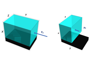
Figure 2: On the left a schematic representation of a soft material in blue, in the initial configuration, on the right the same sample in the current configuration. A normal pressure $P_{0}$ is applied to both surfaces (X,Z) on the left, which becomes $p_{0}$ on the right. For clarity, only one side is shown. To emphasize the deformation, a non-deformable substrate is shown in black and it is assumed that the sample slides on this substrate without friction. Note that the pressure in the reference and current configurations are different due to the expansion of the lateral surfaces.

Assuming a neo-Hookean material with a shear modulus $\mu$ chosen as the unit of stress, then the energy density is $W=1/2(I_{1}-3)$ and the stretch $\lambda_{2}$ is the solution of the cubic equation:

$$\lambda_{2}^{3}+P_{0}\lambda_{2}^{2}-1=0,$$ (18)

which has a unique real root: $\lambda_{2}\sim 1-P_{0}/3$ for small $P_{0}$ and for large compression, the stretch is close to zero so $\lambda_{2}\sim 1/\sqrt{P_{0}}$. Note the simplicity of the derivation of such a solution which, however, implies that the points at the bottom of the cube can slide freely, without friction.

IV Competition between elasticity and continuous fields

Independent of local forces applied to the surface, the shape of a body can change due to different external fields applied and elasticity can be only one cause of the deformation among others. The nonlinear elastic formalism explained above concerns only a part of the global visible deformation and in practice it is not so easy to separate the elastic part from the overall shape. In the case of volumetric growth, each small piece of the sample which initially has a volume $\delta\Omega$ becomes $\delta\omega$ after a growth or drying process that results in a change in the total volume but also in a change in shape or morphology. In the following, the word growth will be used to refer either an increase or a decrease in volume. Furthermore, growth can refer to the cell proliferation, as in embryos, or to the swelling of gels, as already shown in the experiments mentioned in section II. It can also refer to drying or volume decrease.

To separate the growth from the elastic deformation, we keep the definition of the mapping $\chi$ between the initial state and the observed state at time $t$ as it is defined in eq.(1). This mapping gives only a geometric information and we split the tensor ${\bf F}$ into two components: a tensor mimicking the growth $\bf G$ and the tensor ${\bf F_{e}}$ for the elasticity, so that :

$$\bf{F=F_{e}G}\,\,\,\mbox{so}\quad\bf{F_{e}}=FG^{-1}.$$ (19)

This relation, inspired by plasticity modeling and proposed in biomechanics by Rodriguez et al. [94] is local, and ${\bf G}$ is the growth tensor at a point $M$ of the sample, obtained after a period $t$. This law is cumulative in time meaning that the determinant of ${\bf G}$ gives the local amount of growth variation between the initial time and the time of observation. This approach assumes that transient states are quickly eliminated to make room for a slowly adiabatic dependent growth state where the time is an index. Although not intuitive, this formalism actually allows to quantitatively translate some aspects of biological growth, such as inhomogeneity, but also anisotropy of growth: ${\bf G}$ is a tensor, so it simultaneously represents $3$ directions and $3$ eigenvalues, each of them associated with a direction.

A question that immediately comes to mind is the order of the two tensors ${\bf{F_{e}}}$ and ${\bf G}$ when they do not commute. This and other questions have been discussed, see [95]. A physicist would argue that, since the stresses are due to the growth, then the position of ${\bf G}$ is obviously on the right side. Another difficult problem arises simply from the fact that growth is often associated with a process defined per unit time and may be better represented in an Eulerian description while here we are faced with a Lagrangian formulation that relates an initial state to a current state at time $t$. This approach more or less intuitively assumes that the time scale of growth is extremely long compared to any time scale at the origin of the dissipation, reorganization, or remodeling of the samples [96]. Despite its apparent conceptual simplicity, this formalism has generated significant contributions in embryogenesis, morphogenesis and also in the description of various pathologies such as wound healing, fibrosis and tumorogenesis. As suggested by eq.(19), growth induces stresses so not only a change in volume but also a change in its shape and one may wonder if this is always the case. In the next section, we will examine the origin of the stresses induced by growth.

IV.1 The origin of the elastic stresses

IV.1.1 Growth without stress generation

Materials can grow without stress if they can follow and adapt themselves to the imposed growth tensor. This is possible if there are no boundary conditions restricting the growth. Homogeneous growth ${\bf G}=G_{0}{\bf I}$ of a spherical object (without weight) does not generate any stress in the material. If the growth tensor is more complex, e.g. inhomogeneous and anisotropic, the shape of the body will change, as it grows. The question of a stress-free process has recently been explored [97, 98] and examples from living systems have been given. If the deformation of the body can exactly follow the growth process, then ${\bf F=G}$ and is independent of the material properties of the body. Such a relation allows to obtain the tensor ${\bf G}$ and thus the properties of the growth which are mostly unknown for macroscopic samples. This process requires the absence of constraints from boundaries and external forces such as gravity. The best example can be given by fresh planar leaves [99]. To verify such a hypothesis, one possible test is to cut the material at right angles. If there is no crack opening, then the material is considered as stress-free. When the leaves have in-plane residual stresses due to growth, they cannot remain planar, as shown in [74], and they buckle. Recently, a general proof of stress-free growth by conformal mapping was given [100].

IV.1.2 Constrained growth process

Obviously, the main source of stress comes from boundary conditions, especially from rigid walls. Imagine a parallelepiped where only one side is rigidly attached to a substrate and then it cannot evolve freely. This is the case with gels, where the chains of polymers adhere to the substrate, and then mimic clamped conditions. But it is also the case of parallel layers with different elastic properties, that are attached to each other, and grow according to their own rules. The best example concerns growing epithelia, always connected to their ECM (extracellular matrix), such as the imaginal disc of the Drosophila wing [28], the skin layers of the epidermis [101, 102], and also the cortex of the brain connected to the white matter [22, 103], in the embryonic period.
Finally, it is known that life is compatible with elastic stresses, which is the basis of the criterion of homeostasis for mammals: Compressive stress above the homeostatic pressure reduces the cell proliferation, while tensile stress favors the proliferatin.

IV.2 Volumetric Growth and elasticity

The elasticity invariants defined in eq.(2) refer to the elastic tensor ${\bf F_{e}}$ and not to the deformation gradient ${\bf F}$. ${\cal E}$ must now take into account the growth per unit volume of the sample, which is represented by Det $({\bf F})=$ Det $({\bf G})=J$ for an incompressible material, and the elastic energy becomes

$${\cal E}=\int\!\!\!\int\!\!\!\int_{\Omega}dV\,\,J\left\{W(I_{1},I_{2},I_{4},I_{5})-Q\,\,(I_{3}-1)\right\}.$$ (20)

The invariants are given by eq.(2) where ${\bf F}$ is replaced by ${\bf F_{e}}$. In eq.(20) the growth appears explicitly by the factor $J$ which indicates that the material volume has changed and implicitly in the substitution of ${\bf F}$ by ${\bf F_{e}}$ in all the invariants. If we also consider this substitution in the definition of ${\bf S}$ in eq.(10) and of ${\bf\sigma}$ in eq.(14), we have

$${\bf S}=J{\bf G^{-1}}\left\{\frac{\partial W}{\partial{\bf F_{e}}}-Q\,{\bf F_{e}^{-T}}\right\};\,\,{\bm{\sigma}}={\bf F_{e}}\frac{\partial W}{\partial{\bf F_{e}}}-Q\,{\bf I}\,.$$ (21)

In contrast to the Piola stress tensor, ${\bf S}$, the Cauchy stress ${\bm{\sigma}}$ shows no signature of the growth, which can be surprising. At this stage, it is important to emphasize that, first, these two tensors are not defined in the same coordinate basis, and second, only forces acting on a given surface are invariant quantities, as will be shown later. To illustrate this paragraph, we consider a growth process that is anisotropic and the example of section III.4. There is no change in the elastic stretches except for the compressive loading $P_{0}$ which becomes $P_{G}=P_{0}(g_{1}g_{3})$, if we want to keep the same stress level. The stretches do not change and $\lambda_{1}$ is the solution of eq.(18) with $P_{0}$. However, due to the growth, the new coordinates will be: $x_{i}=\lambda_{i}g_{i}X_{i}$.

Now consider the case where the bottom surface of the cuboid is attached to a rigid substrate, assuming anisotropic growth but no applied external compressive stress. Then for $X=0$, the points of this surface cannot move and $y=Y$ and $z=Z$. If no displacement is possible in the $Y$ and $Z$ directions, the simplest choice is to choose the same rules $y=Y$ and $z=Z$, everywhere in the sample, and only the allowed displacements are in the $X$ direction so that $x=JX$. The elastic stretches are then:

$$\lambda_{2}=\frac{1}{g_{2}};\quad\lambda_{3}=\frac{1}{g_{3}};\quad\lambda_{1}=\frac{J}{g_{1}}=g_{2}g_{3}.$$ (22)

According to eq.(21) the Piola stress tensor at the top in the neo-Hookean approach becomes:

$$S_{1}=g_{2}g_{3}\left(g_{2}g_{3}-Q\frac{1}{g_{2}g_{3}}\right)=0;\,\,Q=g_{2}^{2}g_{3}^{2}.$$ (23)

In both horizontal directions, we have:

$$S_{2}=g_{1}g_{3}\left(\frac{1}{g_{2}}-g_{2}^{3}g_{3}^{2}\right);S_{3}=g_{1}g_{2}\left(\frac{1}{g_{3}}-g_{2}^{2}g_{3}^{3}\right).$$ (24)

Note that the horizontal stresses are compressive, which means $g_{i}>1$, indicating that compressive stresses must be applied to the vertical faces at $\pm L_{Y}$ and at $\pm L_{Z}$ to maintain such deformation. Another possibility is an infinite sample in the $Y$ and $Z$ directions. However, growth can also induce a buckling instability which will be studied in detail in the following. When buckling occurs, this simple choice of deformations must be modified, but the main deformation remains for low stress levels above the buckling threshold.
In conclusion, a substrate that prohibits any displacement at the bottom of the parallelepiped is an obstacle to free growth at the origin of compressive stresses, leading eventually to a shape bifurcation.

V Swelling of gels

Swelling hydrogels have the advantage of mimicking the mechanical behavior of growing soft tissue while being precisely controllable. They consist of reticulated networks of polymer chains with a high proportion of small solvent molecules. A phase transition can be induced in the sample when it comes into contact with a reservoir of solvent, resulting in an amazing increase in volume. Although they are perfect candidates for mimicking growing tissues, growth and swelling have different microscopic origins. A swollen hydrogel is a system in both mechanical and thermodynamic equilibrium, and the swelling does not produce any new polymeric components, which constitute the only elastic phase and become increasingly dilute during the swelling process. In addition, the solvent has no reason to be uniformly distributed in the sample. For this reason, different poroelastic models have been proposed for the swelling [104, 105, 106] but also for plant or animal tissues [107, 108, 109, 110, 111]. Here, we choose a presentation by Hong et al. [71, 6] slightly modified to be as close as possible to the section IV.

In fact, at equilibrium, the minimization concerns the grand potential $\hat{\cal W}=\cal W({\bf F},C)-\mu C$ where $C$ is the solvent concentration and $\mu$ is the chemical potential: $\mu=\partial{\cal W({\bf F},C)}/\partial C$. If the gel is in contact with a reservoir full of solvent, then at the interface between the reservoir and the swelling gel, the two chemical potentials in both phases are equal: $\mu=\mu_{s}$. If incompressibility is assumed and can be considered as the sum of its incompressible components, then $C$ is related to Det$({\bf F})$ by the relation: Det$({\bf F})=1+\nu C$, where $\nu C$ is simply the ratio between the volume of the solvent molecules and that of the dry matrix. Obviously, although the experiments on swelling gels are easier to perform and show interesting patterns similar to those observed in nature, we are still faced with two coupled fields: the elastic and the chemical one. Let us consider the variation of the free energy density:

$$\delta\hat{\cal W}=\delta W({\bf F},C)-\mu\delta C=\frac{\partial W}{\partial{\bf F}}\delta{\bf F}+\left(\frac{\partial W}{\partial C}-\mu\right)\delta C\,,$$ (25)

where $\delta C$ is replaced by $\delta$ Det(${\bf F})/\nu$=Det$({\bf F})\,{\bf F^{-T}}\delta{\bf F}/\nu$. Then, the corresponding stress becomes:

$${\bf S}=\frac{\partial W}{\partial\bf{F}}+\frac{1}{\nu}\left(\frac{\partial W}{\partial C}-\mu\right)\text{Det}({\bf F}){\bf F^{-T}}\,.$$ (26)

The free energy density $W({\bf F},C)$ is often represented by the addition of two components: $W_{e}({\bf F})$ and $W_{c}(C)$, where the first represents the elastic energy of the polymer matrix, the second, the contribution $W_{c}(C)$which depends only on $C$. For $W_{e}({\bf F})$, a classical formulation due to Flory and Rehner [112] leads to :

$$W_{e}({\bf F})=\frac{1}{2}NkT\left(I_{1}-3-2Log(\lambda_{1}\lambda_{2}\lambda_{3})\right),$$ (27)

for a compressible polymer matrix that satisfies the neo-Hookean elasticity, $N$ is the number of the polymer chains, while for $W_{c}(C)$ we have:

$$W_{c}(C)=-\frac{kT}{\nu}\left(\nu CLog[\frac{(1+\nu C)}{\nu C}]+\frac{\Upsilon}{1+\nu C}\right).$$ (28)

If we consider the case of a cuboid with clamped conditions at the bottom, then we can again imagine a diagonal strain and stress tensors with $\lambda_{2}=\lambda_{3}$ and ${\bf F}_{11}=\lambda_{1}$ , so that

$$S_{1}=NkT\left\{\lambda_{1}-\frac{1}{\lambda_{1}}-\frac{1}{N\nu}\lambda_{2}^{2}\left(w^{\prime}+\frac{\mu}{kT}\right)\right\}=0\,,$$ (29)

$$S_{2}=NkT\left\{\lambda_{2}-\frac{1}{\lambda_{2}}-\frac{1}{N\nu}\lambda_{1}\lambda_{2}\left(w^{\prime}+\frac{\mu}{kT}\right)\right\},$$ (30)

with

$$w^{\prime}=-\left(Log(\frac{\lambda_{1}-1}{\lambda_{1}})+\frac{1}{\lambda_{1}}+\frac{\Upsilon}{\lambda_{1}^{2}}\right),$$ (31)

and a similar result for $S_{3}$, which is equal to $S_{2}$. The relative increase of the height $\lambda_{1}$ in the vertical direction leads to a compressive stress in the horizontal directions, at the origin of the buckling of the sample. Here the control parameter is $\mu/\nu$ at the origin of the swelling/deswelling. Although there is an analogy between volumetric growth and swelling, the theoretical approach will be more uncertain in the second case and also more dependent on the experimental conditions. Therefore, for our purposes, and in the following, we will restrict ourselves to the simplest initial geometry and suggest how we can interpret the experiments shown in section II.

VI Biot’s theory applied to rubber in compression versus volumetric growth

VI.1 Compression and critical instability threshold

Thick samples can buckle under compression. This volumetric instability occurs when the compressive stresses due to load reach a threshold value. In fact, as mentioned in section II, experimentalists often characterize buckling by the compressive strain $\lambda_{2}$ rather than by the compressive load. In fact, strain, which is the ratio of the length of the speciment to the initial length, is more easily evaluated. Biot has studied this buckling instability in detail, in particular for the neo-Hookean and Mooney-Rivlin models for a semi-infinite sample representing a free surface, subjected to a lateral compression, which we will call $P_{0}$. This simple geometry allows a diagonal representation of the strains and stresses before the bifurcation, and this instability is often called a surface instability because it is more easily observed at the surface. His proof concerns a simple plane strain instability controlled by a parameter $\xi$, above which the simple diagonal representation ceases to be valid. $\xi$ and $\xi_{B}$ are given by:

$$\xi=\frac{\lambda_{1}^{2}-\lambda_{2}^{2}}{\lambda_{1}^{2}+\lambda_{2}^{2}}\quad\mbox{and}\quad\xi_{B}=0.839287.$$ (32)

For the neo-Hookean model, Biot [23] has established the following relation for $\xi_{B}$:

$${\cal Q}_{B}=\xi_{B}^{3}+2\xi_{B}^{2}-2=0\,.$$ (33)

We will consider three different cases, the first two were considered in [113]. The stresses are defined in the current configuration and ${\bm{\sigma}}$ represents the Cauchy stress. In the following three cases there is no stress on the top free surface, which leads to : $\sigma_{1}=\lambda_{1}^{2}-Q=0$ when the shear modulus is chosen as unity: $\mu=1$. It gives $Q=\lambda_{1}^{2}$. Remember that in this case $\sigma_{1}-\sigma_{i}=-\sigma_{i}=\lambda_{1}^{2}-\lambda_{i}^{2}$  for $i=2$ or $3$.

VI.1.1 Case one

We assume that there is no strain in the $Z$ direction and $\lambda_{3}=1$

$${\bf F}=\rm{Diag}(\lambda_{1},\lambda_{2},1);\,\,{\bm{\sigma}}=\rm{Diag}(0,\lambda_{2}^{2}-\lambda_{1}^{2},1-\lambda_{1}^{2}).$$ (34)

With this choice, incompressibility imposes: $\lambda_{2}=1/\lambda_{1}$ and the parameter $\xi$ becomes:

$$\xi=\frac{\lambda_{1}^{2}-1/\lambda_{1}^{2}}{\lambda_{1}^{2}+1/\lambda_{1}^{2}}\quad{\mbox{so}}\quad\lambda_{1}=\left(\frac{1+\xi}{1-\xi}\right)^{1/4}.$$ (35)

At the threshold of stability, the value of the stretches are then given by $\xi=\xi_{B}$, and $\lambda_{1}=1.839287$ so $\lambda_{2}=0.543689$, and compressive stresses occur in both directions for $Y$ with $\sigma_{2}=-3.0873$ and for $Z$  with $\sigma_{3}=-2.38298$.

VI.1.2 Case two

Choosing now $\lambda_{1}=\lambda_{3}$

$${\bf F}=\rm{Diag}(\lambda_{1},\lambda_{2},\lambda_{1})\quad{\bm{\sigma}}=\rm{Diag}(0,\lambda_{2}^{2}-\lambda_{1}^{2},0)\,.$$ (36)

With this choice, the incompressibility imposes: $\lambda_{2}=1/\lambda_{1}^{2}$ and the parameter $\xi$ and $\lambda_{1}$ become:

$$\xi=\frac{\lambda_{1}^{2}-1/\lambda_{1}^{4}}{\lambda_{1}^{2}+1/\lambda_{1}^{4}}\quad{\mbox{so}}\quad\lambda_{1}=\left(\frac{1+\xi}{1-\xi}\right)^{1/6}\,,$$ (37)

which gives the instability when $\lambda_{1}=1.50118$ and $\lambda_{2}=0.443746$. The compressive stress occurs only in the $Y$ direction with $\sigma_{2}=-2.05663$.

VI.1.3 Case three

Finally for the third case, we assume that the compressive loads act similarly in both directions: $Y$ and $Z$.

$${\bf F}=\rm{Diag}(\lambda_{1},\lambda_{2},\lambda_{2});\,\,{\bm{\sigma}}=\rm{Diag}(0,\lambda_{2}^{2}-\lambda_{1}^{2},\lambda_{2}^{2}-\lambda_{1}^{2}).$$ (38)

With this choice, incompressibility imposes $\lambda_{2}=1/\sqrt{\lambda_{1}}$ and the parameter $\xi$ and $\lambda_{1}$ become:

$$\xi=\frac{\lambda_{1}^{2}-1/\lambda_{1}}{\lambda_{1}^{2}+1/\lambda_{1}}\quad{\mbox{so}}\quad\lambda_{1}=\left(\frac{1+\xi}{1-\xi}\right)^{1/3},$$ (39)

which gives the instability when $\lambda_{1}=2.25354$ and $\lambda_{2}=0.666142$ and a compressive stress equal in $Y$ and $Z$ direction: $\sigma_{2}=\sigma_{3}=-4.6347$. Note that this last case is not considered by Biot.

VI.2 Semi-infinite samples under volumetric growth

As shown earlier, the Biot instability is mostly controlled by the strains that are directly observable for a solid under compression. There is no difference between the elastic and the geometric strains as opposed to growth. Assuming that the previous analysis remains valid, we will try to apply the Biot approach to volumetric growth. To do so, we will reconsider the three cases defined above.

VI.2.1 Case one

This case concerns $\lambda_{3}=1$, which means that in this direction the displacement is equal to growth. Then the critical elastic strains evaluated in section VI.1.1 are equal to $\lambda_{1}\sim 1.839$ and $\lambda_{2}=0.543689$. There are several cases depending on how the growth is organized in the sample. For isotropic growth without displacement in the $Y$ direction, we have $x=JX$, $y=Y$ and $z=gZ$ with $\lambda_{1}=J/g$, $\lambda_{2}=1/g$ and $J=g^{2}$. So the expansion in the $X$ and $Z$ direction at criticality is $g=1.839$. These values were determined directly in [19] and are recovered in a different way in section VII. The compressive stresses in the $Y$ and $Z$ directions become: $\sigma_{2}=-3.0874$ and $\sigma_{3}=-2.383$. $J$ can be evaluated by noting that $\xi=(J^{2}-1)/(J^{2}+1)$ which once introduced into eq.(33) leads to the polynomial for $J_{B}$:

$${\cal Q}_{J}=J_{B}^{3}-3J_{B}^{2}-J_{B}-1=0;\,\,J_{B}=3.38298\,.$$ (40)

This configuration will be examined in detail in all the following sections.

VI.2.2 Case two

This case concerns the growth of a sample with $2$ sides  without stress. Assuming $x=J_{1}X$, $y=J_{2}Y$ and $Z=J_{1}X$, then at the threshold $\lambda_{1}=J_{1}/g=\lambda_{3}=1.5012$ and $\lambda_{2}=J_{2}/g=0.4437$ with $g$ defined as $g^{3}=J_{1}^{2}J_{2}$. There is only a compressive stress in the $Y$ direction with the same value as in section VI.1.2: $\sigma_{2}=-2.0567$

VI.2.3 Case three

In this case it is assumed that $x=J_{1}X$, $y=J_{2}Y$ and $z=J_{2}Z$. If the displacement is forbidden along the $Y$ and $Z$ directions, then $J_{2}=J_{3}=1$ and $J=J_{1}=g^{3}$.

$$\begin{cases}{\bf G}=\rm{Diag}({g,g,g)};\\ {\bf F}=\rm{Diag}(\frac{J_{1}}{g},1,1);\\ {\bf F_{e}}=\rm{Diag}(\frac{J_{1}}{g},\frac{1}{g},\frac{1}{g});\\ {\bm{\sigma}}=\rm{Diag}(0,\frac{1}{g^{2}}-g^{4},\frac{1}{g^{2}}-g^{4})\,.\end{cases}$$ (41)

This unidirectional growth process produces lateral compressive stresses when $g$ and $J_{1}$ are greater than one. In the opposite case $J_{1}<1$, the stresses are tensile. This case is similar to eq.(38) and

$$\xi_{B}=\frac{g^{4}-1/g^{2}}{g^{4}+1/g^{2}}=\frac{J_{1}^{2}-1}{J_{1}^{2}+1}\,.$$ (42)

At the threshold, replacing $\xi_{B}$ by $J_{B}$ in eq.(33) we obtain the critical threshold for such growth process given by:

$${\cal Q}_{J}=J_{B}^{3}-3J_{B}^{2}-J_{B}-1=0\,.$$ (43)

The solution for $J_{B}$ is then $J_{B}=3.38298$, the critical strain is then $\lambda_{1}=2.25354$ and $\lambda_{2}=0.666142$. Note that we recover the same threshold for the growth parameter as for section VI.2.1.
Growth anisotropy increases the space of possible instability parameters. Here we limit ourselves to three cases and restrict ourselves to homogeneous growth. The Biot instability is generic, but depending on the situation, the thresholds can be different and must be evaluated each time. In the following, we will consider only one case with a different theoretical approach, without using the Biot’s method, which imposes a critical parameter $\xi_{B}$ [23]. We prefer a presentation in terms of variational analysis.

VII Growth of a semi-infinite sample

It is impossible to list all the publications on volumetric growth in soft matter. If growing layers, multilayers, shells, disks, spheres are the most frequently chosen geometries [21], numerical treatments with advanced finite elements methods softwares allow to represent a variety of shapes closer to reality [114]. Our purpose is different since we want to give exact results with the simplest and standard hyperelastic model, that is the neo-Hookean model [93, 91, 21] for incompressible materials. In addition, instead of considering all possible growth processes that can be found in nature, anisotropic [7] or space dependent [97, 98], we focus on a spatially constant growth that evolves on a rather long time scale in order to neglect any transient dynamics. Since elasticity goes hand in hand with geometry [89], we start with the geometry of the sample to fix the notations used in the following.

VII.1 The geometry

We consider a semi-infinite growing sample bounded by the plane $X=0$, infinite in the positive $X$ direction and extending laterally between $-\infty,\infty$ in the $Y$ and $Z$ directions. We assume $\lambda_{3}=1$, so that no elastic strain exits in the third direction. The growth is assumed to be isotropic and homogeneous with a constant relative volume expansion $J=g^{3}$. Due to the Biot instability (see the previous section), periodic patterns will appear on top of the sample with a spatial periodicity $\Lambda$ chosen as the length unit. This geometry orients the growth mostly in the $X$ direction and the new position for an arbitrary material point inside the sample leads to compressive stresses in the $Y$ direction, as described before in section VI.2.1. Thus, defining a Cartesian coordinate system $X,Y$ in the initial configuration, the position of each point after growth and the elastic deformation becomes $x\sim JX$ and $y\sim Y$, in leading order and $J_{2D}=J=g^{2}$. Since an adiabatic approach to the growth process is assumed, i.e. transient deformations are quickly eliminated, a free energy describes the possible patterns resulting from a symmetry breaking. Our approach, which is poorly followed in the mechanics community, will be based on energy variation and will avoid tensorial algebra.

VII.2 The variational method based on the free energy minimization

VII.2.1 The free energy: elasticity and capillarity

The Euler-Lagrange equations or the equilibrium equations result from the extremum of the free energy, the sum of the elastic and possibly surface energy. Assuming a perfect periodicity of the patterns, we make a virtual partition of the initial domain into stripes of unity width and focus on ${\cal P}$  the domain between $-1/2<Y<1/2$, see the blue domains in Fig.(3). The neo-Hookean model depends on only two invariants: $I_{1}$, for the elastic deformations and $I_{3}$ for the relative volume change due to elastic stresses, which we renormalize into the geometric invariants: $\tilde{I}_{1}=JI_{1}$ and $\tilde{I}_{3}=JI_{3}$ :

$$\tilde{I}_{1}=x_{X}^{2}+x_{Y}^{2}+y_{X}^{2}+y_{Y}^{2}-2J;\tilde{I}_{3}=x_{X}y_{Y}-y_{X}x_{Y}-J\,,$$ (44)

where the subscript $X$ (resp. $Y$) denotes the partial derivative of any function with respect to the variable $X$ (resp. $Y$).
The invariants $I_{1}$ and $I_{3}$ have already been defined in section III.2. The energy unit is chosen as the product: $\mu\cdot(\Lambda^{2}t_{3})$. $t_{3}$ is the thickness of the sample in the orthogonal direction which is irrelevant for plane strain deformations and we have for the elastic energy of a single strip:

$${\cal E}_{e}=\frac{1}{2}\iint_{{\cal P}}dS\left(\tilde{I}_{1}-2Q\tilde{I}_{3}\right).$$ (45)

The Lagrange parameter $Q$ is also a function of $X$ and $Y$ fixing the incompressibility constraint $I_{3}=1$ or $\tilde{I}_{3}=0$ and $dS=dXdY$. The capillary energy is often written in Eulerian coordinates:

$${\cal\tilde{E}}_{c}=\gamma_{0}\int_{\partial{\cal P}}dy\sqrt{1+x_{y}^{2}}\,.$$ (46)

Considering the upper boundary $\partial{\cal P}$:

$$X=0;\quad Y\in[-1/2,1/2],$$

where the capillary energy is defined, the following relations hold :

$$dy=\frac{\partial y}{\partial Y}|_{{}_{X=0}}\,dY\quad\mbox{and}\quad dx=\frac{\partial x}{\partial Y}|_{{}_{X=0}}\,dY,$$ (47)

then eq.(46) is transformed into:

$${\cal E}_{c}=\gamma_{0}\int_{\partial{\cal P}}dY(\sqrt{x_{Y}^{2}+y_{Y}^{2}}-1)\,,$$ (48)

where $\gamma_{0}$ is the rescaled capillarity coefficient and is equal to $\gamma_{0}=\gamma/(\mu\Lambda)$ ( $\gamma$ is the surface tension). Capillarity represents the average energy difference between the microscopic components of the sample (as atoms, molecules) located in the bulk or at the interface. It is positive when the interface separates a dense material from a more dilute phase. In practice, the capillary coefficient $\gamma_{0}$ is very weak for ordinary gels and plays a significant role only when the sample size is of the order of $0.1$mm and for extremely soft gels [115].  However a skin effect can occur on top of elastic samples due to inhomogeneity of the shear modulus or to the growth process itself. This is especially true for the swelling of gels. Despite the weakness of this energy, it plays a crucial role in the determination of the wavelength and in the local regularization of singular profiles.

VII.2.2 The Euler-Lagrange equations

They simply result from the first variational derivative of the functional ${\cal E}_{e}$ with respect to the small variation of $x$ and $y$:

$$\begin{cases}x_{XX}+x_{YY}=Q_{X}\,y_{Y}-Q_{Y}\,y_{X}=\{Q,y\}\,,\\ y_{XX}+y_{YY}=-Q_{X}\,x_{Y}+Q_{Y}\,x_{X}=-\{Q,x\}\,.\end{cases}$$ (49)

The left-hand side of the equation (49) represents the Laplacian $\Delta$ in Cartesian coordinates, and $\{P,x_{i}\}$ is the Poisson bracket of $P$ and $x_{i}$. This mathematical symbol has important properties in mechanics [116]. The zero-order solution : $x=JX$ and $y=Y$ verify these equations when the Lagrange parameter is a constant, so $Q=Q_{0}$. Boundary conditions are also derived from the first variational derivative of ${\cal E}_{e}$ and ${\cal E}_{c}$ with respect to the elementary variation of $x$ and $y$, a process which allows the cancellation of the normal components $S_{11}$ and $S_{21}$ of the Piola stress tensor $\bf S$ [93, 91], at the free boundary $\partial{\cal P}$:

$$S_{11}=x_{X}-Q\,y_{Y}\quad\mbox{and}\quad S_{21}=y_{X}+Q\,x_{Y}\,.$$ (50)

On top, for $X=0$, the cancellation of $S_{11}$ gives $Q_{0}=J$ while $S_{21}=0$ is automatically obtained for the zero order solution. Capillarity appears for buckled solutions and is responsible for the normal $\Gamma_{11}$ and tangential $\Gamma_{21}$ components:

$$\Gamma_{11}=\gamma_{0}\frac{\partial}{\partial Y}\frac{x_{Y}}{(x_{Y}^{2}+y_{Y}^{2})^{1/2}}\,,$$ (51)

and

$$\Gamma_{21}=\gamma_{0}\frac{\partial}{\partial Y}\frac{y_{Y}}{(x_{Y}^{2}+y_{Y}^{2})^{1/2}}\,,$$ (52)

which must be added to the normal stresses at $X=0$. Note the strong nonlinearities in the surface energy. However, since $\gamma_{0}$ is in practice a very small parameter, the role of the capillary stresses is probably negligible for smooth patterns, but may become important in the case of creases. For completeness, the other two components of the stresses are also given:

$$S_{12}=x_{Y}+Q\,y_{X}\quad\mbox{and}\quad S_{22}=y_{Y}-Q\,x_{X}\,.$$ (53)

So far, it is assumed that the interface is regular and admits a regular curvature everywhere. Self-contacting interfaces are not considered, although in the last panel (A9)of Fig(1) on the right, such a property can explain the highly singular pattern obtained in the radial geometry. Assuming that it happens at a position $Y=0$, then two additive stress boundary conditions must be imposed locally [38, 39, 40],

$$S_{22}|_{Y=0^{+}}=S_{22}|_{Y=0^{-}}\,\,{\mbox{and}}\,\,S_{12}|_{Y=0^{+}}=S_{12}|_{Y=0^{-}},$$ (54)

the second condition indicates the absence of friction on the singular line.
Finally, it is easy to show that the Euler-Lagrange equations, eq.(49), are equivalent to the cancellation of the divergence of the Piola stress tensor, see also section III.3 and eq.(12). In Cartesian coordinates, Div$({\bf S})_{i}=\partial Sij/\partial X_{j}$.

VII.3 Incremental approach and solution of the Euler-Lagrange equations

The classical way to detect a bifurcation in the elasticity is to expand the general solution by adding a small perturbation scaled by a small parameter $\epsilon$. The following results are obtained for $x$ and $y$ and $Q$ :

$$\begin{cases}Q=J+\epsilon q(X,Y)\,,\\ x=JX+\epsilon U(X,Y)\quad\mbox{with}\quad\Delta U=q_{X}\,,\\ y=Y+\epsilon V(X,Y)\quad\mbox{with}\quad\Delta V=Jq_{Y}\,.\end{cases}$$ (55)

The incompressibility condition at $\epsilon$ order imposes the following constraint $U_{X}+JV_{Y}=0$ and the elimination of $q$ is easy by cross-derivation of the previous equations, eq.( 55): $J\partial_{Y}\Delta U-\partial_{X}\Delta V=0$ which can be derivated a second time to isolate $U$ from $V$. Defining $\Delta_{J}=\partial^{2}_{XX}+J^{2}\partial^{2}_{YY}$:

$$\Delta_{J}(\Delta U)=\Delta_{J}(\Delta V)=0.$$ (56)

and $\Delta_{J}q=0$. The fourth order operator $\Delta_{J}\Delta=\Delta\Delta_{J}$ accepts as possible solutions $\Re\,(\Phi_{1}(Z)+\Phi_{2}(Z_{1}))$ where both functions are holomorphic functions of $Z=X+IY$ and $Z_{1}=JX+IY$. Nevertheless, due to the boundary conditions for $X=0$ (on the top of the strip), $\Phi_{1}$ and $\Phi_{2}$ are related and we finally get for $x$ and $y$:

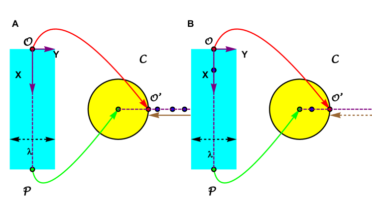
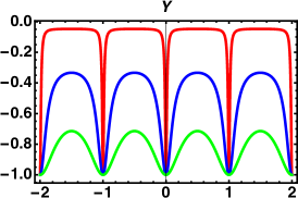
(a)  Profile for an outer pole

(b)  Real Part

(c)  Imaginary part

Figure 3: At the top, panels A and B, the physical domain ${\cal P}$, corresponding to one wavelength in cyan, is restricted to $-1/2\leq Y\leq 1/2$, $X\in[0,+\infty]$. Only one wavelength is plotted. To the right of each panel, is the ${\cal C}$ plane with the unit Riemann disk in yellow. The red arrow indicates the correspondence between the point $\mathcal{O}$ ( $X=0,Y=0$ ) of the physical space and the point $\mathcal{O^{\prime}}$ (${1,0}$) of the ${\cal C}$ plane. The region $X->+\infty$ is contracted and associated with the center of the Riemann disk (green arrow). Only the interior and the contour of the Riemann disk mimic the physical domain. The blue dots represent the possible singularities, which are not singular for the physical domain in panel (A), but can generate sharp interface variations. Note that the dashed purple lines are images of each other due to the conformal mapping. In (B), the same plot except that a singular point enters both the Riemann disk and the physical plane P. Below, in (b), the interface profile for an outer pole, see eq.(63), with the parameter $a=0.1$ for the red curve, $a=1$ for the blue curve, $a=5$ for the green curve. The profile appears quite singular for $a=0.1$, but it remains finite. In (c) the real part of the derivative which contributes to the stresses, see $S_{11}$, according to eq.(58). One wavelength, ${\mathcal{P}}$, is shown and the rainbow colors indicate the sharp variations near the origin $\mathcal{O}$. Note also that the scale for $X$ varies between $0$ and $0.1$. Although quite singular near $\mathcal{O}$, the stress remains finite and decreases rapidly. Similarly, (d) shows the opposite of the imaginary part present in $S_{21}$ of eq.(58).

$$\begin{cases}x&=JX+J\epsilon\Re\,[\Phi(Z)+\tau_{1}\Phi(Z_{1})]\,,\\ y&=Y-\epsilon\Im\,[\Phi(Z)+J\tau_{1}\Phi(Z_{1})]\,,\\ Q&=J+\epsilon\tau_{0}\tau_{1}\Re\,[\Phi_{Z_{1}}];\,\,\tau_{0}=J^{2}-1\,,\end{cases}$$ (57)

where $\Re\,$ and $\Im\,$ are the real and imaginary parts of the holomorphic function $\Phi$. The notation $\tau_{0}=J^{2}-1$ is introduced for convenience and $\tau_{1}$ is free at this stage, and will be determined later. A priori $\Phi$ is arbitrary with the restriction that it must vanish for $X\rightarrow\infty$ which automatically implies that $\Phi$ is singular. Any singularity occurring outside of the domain ${\cal P}$ (for $X<0$) is physically appropriate while singularities within the physical domain ${\cal P}$ must be considered with caution. The balance of the elastic and capillary stresses at the surface $\partial{\cal P}$ gives the value of $\tau_{1}$ as well as the threshold $J_{B}$ for the buckling instability. Let us first evaluate the stresses in linear order in $\epsilon$: The calculation is not difficult and can be easily done using the Mathematica software as an example (see also the Appendix, section XV.1):

$$\begin{cases}S_{11}&=\epsilon\Re\,[2J\Phi_{Z}+(1+J^{2})\tau_{1}\Phi_{Z_{1}}]\,,\\ S_{21}&=-\epsilon\Im\,[(1+J^{2})\Phi_{Z}+2J^{2}\tau_{1}\Phi_{Z_{1}}]\,,\\ S_{12}&=-\epsilon J\Im\,[2\Phi_{Z}+(1+J^{2})\tau_{1}\Phi_{Z_{1}}]\,,\\ S_{22}&=1-J^{2}-\epsilon\Re\,[(1+J^{2})\Phi_{Z}+2J^{3}\tau_{1}\Phi_{Z_{1}}]\,.\end{cases}$$ (58)

Only $S_{22}$ shows a zero order contribution in $(-\tau_{0})=1-J^{2}$, which is negative for a growing material since $J>1$. This compressive stress explains the buckling instability and is associated with an elastic strain along $Y$.

VII.4 The boundary conditions at the top of the sample, the Biot threshold and the harmonic modes

To derive the condition of a buckling instability, the quantities of interest are the normal $S_{11}$ and shear $S_{21}$ stresses at the top, which must include the capillary contribution. Only the normal capillary stress $\Gamma_{11}$ is of order $\epsilon$ while $\Gamma_{21}$ is of order $O(\epsilon^{2})$ and can be discarded so it reads, for $X=0$ and for $S_{11}$:

$$\epsilon\left(2J+(1+J^{2})\tau_{1}\right)\cdot\Re\,[\Phi_{Z}]-\epsilon\gamma_{0}J(1+\tau_{1})\Re\,[\Phi_{ZZ}]\,,\\$$ (59)

where $\tau_{1}$ is not modified. We first neglect the surface tension. Then, the cancellation of $S_{21}$ gives the value of $\tau_{1}$: $\tau_{1}=-(1+J^{2})/(2J^{2})$. Once this $\tau_{1}$ value is introduced into $S_{11}$, there are two possibilities:

• Cancellation of ${\cal Q}(J)$, leading to the determination of $J_{B}$ such that :

  $${\cal Q}(J_{B})=(J_{B}^{3}-3J_{B}^{2}-J_{B}-1)=0\,,$$ (60)

  for any profile function $\Phi(Z)$. This value was also found by Biot, see section VI.2.1 where another demonstration by Biot is proposed  [113] .
  

• $\Re\,[\Phi_{Z}]=0$ which defines a family of suitable profiles but not a threshold value for observing the interface buckling. It requires that $\Phi$ is an even function of $Z$.

The second case does not imply any specific value of $J$, but selects shape profiles, unlike the first case which occurs above $J_{B}$ for any profile. It suggests and explains the diversity of experimental observations for the layer buckling: Indeed, the absence of mode selection at the Biot threshold automatically induces a spontaneous coupling of harmonic modes. The only real root $J_{B}$ of ${\cal Q}(J)$ is

$$J_{B}=\frac{1}{3}(3+6^{1/3}\{(9-\sqrt{33})^{1/3}+(9+\sqrt{33})^{1/3}\})\,,$$ (61)

$J_{B}\sim 3.38$. But, as mentioned above, all holomorphic periodic functions of $Z$ that vanish for $X\rightarrow+\infty$ are possible eigenmodes of deformations that occur for the same threshold value. In the original papers, Biot only focused on the harmonic modes: $\Phi_{B}=e^{-2\pi nZ}$, which appear for a compressed rubber sample. The polynomial that gives the threshold is not always the same depending on the experiment. Any modification in the physics of the problem such as more sophisticated hyperelasticity (Mooney-Rivlin, Ogden model, Fung-model [93, 91], anisotropy of the material [90] or of the growth [7, 8], possibly external loading, will modify the incremental result eq.(57) and the critical polynomial $\cal{Q}$, but not the fundamental property of instability.

However, this model does not provide a choice of wavelength at the threshold, unlike the similar instabilities of fluids such as Rayleigh-Bénard or Bénard Marangoni [34]. Above the threshold, the determination of the wavelength for periodic fluid instabilities remains a difficult theoretical challenge [117, 34, 118] giving rise to an important literature and sometimes controversies as for the Rayleigh-Bénard convection or the diffusion patterns of directional solidification. In [19], a surface tension selection mechanism is proposed for a layer of finite height $d$. It induces a shift of the threshold $J_{B}$ and a selection of the ratio: wavelength over the height $d$ of the sample, this ratio being of order one. Here the sample height is infinite and the wavelength is chosen as length unit, which means that the selection must in principle provide the value of the critical threshold $J_{C}$. A discussion of finite size effects is deferred to the last section XIII. When capillarity is introduced, the normal stress $S_{11}$ and the shear stress $S_{21}$, given by eq.(59) are modified by the capillary contribution. Only the periodic function $\Phi=e^{-2n\pi Z}$ (where n is an integer) gives a simple solution with a shift of the bifurcation threshold due to $\Gamma_{11}$:

$$\delta J=J_{C}-J_{B}=n\pi\gamma_{0}J_{B}\frac{(1+J_{B})}{(3J_{B}^{2}-6J_{B}-1)}\,.$$ (62)

It is possible to recover this threshold directly minimizing the the total energy: elastic and capillary energy. In the next section, we give examples of such an evaluation which takes advantage of the expansion given in section XV.2.

VIII Periodic profiles and the Riemann theorem

VIII.1 Construction of periodic profiles

The choice of the periodic functions $\Phi(Z)$ follows from the Riemann theorem, which states that there exists a bijective mapping between a non-empty and simply connected domain and the unit disk   ${\cal C}$. In our case the domain is ${\cal P}$, which covers one period, see Fig.(3). Introducing the complex variable $\zeta=e^{-2\pi Z}$, Fig.(3) shows the points of correspondence, in particular the upper boundary ($X=0$) of $\partial{\cal P}$, which is mapped onto the outer circle $\partial{\cal C}$, and the zone at infinity of ${\cal P}$ ($X\rightarrow+\infty$) concentrated in the center of the unit disk. The exterior of the unit disk corresponds to the non-physical half-plane where $X<0$. The central vertical axis of the strip $X>0,Y=0$, (dashed purple line in Fig.(3)) is associated with the horizontal axis of the ${\cal C}$ plane (purple dashed lines) which we extend into the non-physical domain. Every holomorphic function, except constants, $\Phi(Z)$ or $\Psi(\zeta)$, has singularities. If they are located in the non-physical plane, these solutions are physically relevant, since they contribute to a finite elastic energy density. But this is not the case when they are located inside ${\cal P}$ or ${\cal C}$, where they require special attention. When they are near the boundary or of the Riemann circle $\partial{\cal C}$, they become good candidates for generating creases. We will consider the regular profiles first.

VIII.2 Regular patterns above the Biot threshold.

The patterns of interest are of course the harmonic modes $\zeta_{k}=e^{-2\pi kZ}$ and their superposition:  $\Phi(Z)=a_{k}\zeta^{k}$ where the Einstein notation on double indices is assumed and with $k$ a positive integer. The Biot solution is simply $\zeta=e^{-2\pi Z}$. All these modes without specific parity in the change $Z\curvearrowright-Z$ occur strictly at the Biot threshold and can easily overlap. However, when focusing on folds occurring at the interface, a more appropriate choice must be made with singularities located near the interface. The word creases is chosen to describe a sharp and localized variation of the interface shape $\partial{\cal P}$, which is mathematically represented by a continuous function, such that the profile $x(Y)$ remains differentiable, at least $2$ times. Another definition can be that the elastic and/or capillary energy density remains locally finite. A fancy representation in complex analysis has been given by the viscous interfacial flow experts. [119, 120, 54, 121]. The creases are then simply generated at the threshold by using the conformal mapping technique [122, 123]. Defining the neighborhood of the central line $\zeta_{a}=\zeta-1-a$, with $a>0$, possible solutions with a pole, a logarithm or a square root can be good representations of quasi-singular profiles in the neighborhood near the center of the strip $\mathcal{O}$ or near $\mathcal{O^{\prime}}$:

$$\Phi=\frac{a}{\zeta_{a}};\,\,\Phi=-\frac{Log(-\zeta_{a})}{Log(a)};\,\,\Phi=(-\zeta_{a})^{1/2}\,,$$ (63)

$a$ decreases as one approaches the point $\mathcal{O^{\prime}}$, or the interface near $\mathcal{O}$ (see Fig.(3)). The amplitude of the singular profile is normalized in the definition given by eq.(63). Fig.(3) shows different profile solutions for $a=0.1$ (red curve), $a=1$ (blue curve) and $a=5$ (green curve) for a pole singularity (first choice of eq.(63) on the left) corresponding to a distance $d_{a}$ from the point $\cal{O}$ of the physical plane with $d_{a}=-0.0152,-0.110,-0.285$ respectively. Since $\Phi_{Z}$ goes directly in the stress definition, its value gives information about the stresses, see eq.(58) and Fig.(3), panels (c)  and (d). Plotted on a single wavelength $-0.5<Y<0.5$ (with $a=0.1$), the real and imaginary parts of $\Phi$ show a strong localization near the interface for $a=0.1$ so $d_{a}=0.0152$ and they quickly disappear with increasing values of $X$. However, even if the stresses at the interface are large, the solution is not singular and the linear expansion remains valid for sufficiently small values of $\epsilon$. For the logarithm or square root choices presented in eq.(63), see the Appendix (XV.4).

VIII.3 The case of even holomorphic function of $Z$

The second way to satisfy the cancellation of the stress $S_{11}$ for $X=0$ is to choose an even function of $Z$, which means that $\Phi(Z)=a_{k}(\zeta^{k}+\zeta^{-k})$ which will automatically diverge in the center of the Riemann disk or at infinity of ${\cal P}$. The only way to satisfy the convergence at infinity is to introduce a singularity inside the Riemann disk. The choice of such a singularity is huge, but $2D$ elasticity allows only logarithm and square root singularities for elastic energy convergence. In linear elasticity, it is well known that square roots c correspond to fractures and logarithms to wedge dislocations, see [124]. Before proceeding further in this direction, let us start with the nonlinear coupling of regular modes.

IX Nonlinear bifurcation analysis via energy minimisation and mode coupling

All modes emerge at the Biot threshold and the mechanisms of selection are never a simple matter in the physics of continuous media. For example in diffusion-limited growth, the selection of the size and velocity of the needle-crystal remained a puzzle for five decades. In fact, Ivantsov [125, 126, 127, 128] has demonstrated the relationship between the tip radius of the crystal times its velocity as a function of the undercooling since $1947$ but disentangling both quantities by the appropriate correct physical process has generated many conflicting hypotheses and discussions. The role of the surface tension, much debated due to mathematical difficulties, is now understood by including the surface tension anisotropy   [61, 129]. In the same class of problems, the displacement of a viscous finger in a channel remains unsolved for about thirty years [130] and it has been again demonstrated the role of the surface tension which chooses a discrete set of solutions among a continuum [56, 57, 55]. When an energy emerges, as in our formulation of volumetric growth, solutions can be selected by an energy minimization, which was not the case for the two examples mentioned above. However our continuum here is a continuum of possible functions, not just a selection of a pure number characteristic of the pattern. Using an expansion of the deformation at $\epsilon$ order, the energy density can be expanded in $E=\tau_{0}/2+\delta E$, as follows:

$$\delta{\cal E}=\epsilon\int_{{\cal P}}dS(E_{1}+\epsilon E_{2}+\epsilon^{2}E_{3})=\epsilon{\cal E}_{1}+\epsilon^{2}{\cal E}_{2}+\epsilon^{3}{\cal E}_{3}\,,$$ (64)

where each order is given in the Appendix (XV.2).

If the system is governed by an energy, it is a possible to analyze the bifurcation in more detail, to deduce its characteristics and finally to obtain the amplitude $\epsilon$ of the selected mode by expanding the energy. To prepare such a calculation, which can be really tedious and even impossible for an arbitrary choice of $\Phi$, we take advantage of the complex formulation.

IX.1 Elastic energy evaluation, order by order

Such an evaluation requires surface integrals covering the entire domain of interest ${\cal P}$ (Fig.(4), top left panel) which can be obtained in two ways: either in $X,Y$ coordinates, or in $Z,\bar{Z}$ coordinates. The latter choice makes the calculus much more easier for the first and second order, as soon as holomorphic functions are chosen in the rectangular geometry. First, we define these surface integrals defined on ${\cal P}$ as:

$$\begin{cases}K^{(1)}(f,\bar{g})=\frac{1}{2I}\iint_{{\cal P}}dZd\bar{Z}f_{Z}\bar{g}_{\bar{Z}}\,,\\ K^{(2)}(f_{1},\bar{g}_{1})=\frac{1}{2JI}\iint_{{\cal P}}dZ_{1}d\bar{Z}_{1}f_{Z_{1}}\bar{g}_{\bar{Z}_{1}}\,,\\ K^{(3)}(f\bar{g}_{1})=\frac{1}{I(J+1)}\iint_{{\cal P}}dZd\bar{Z}_{1}f_{Z}\bar{g}_{\bar{Z}_{1}}\,,\\ K^{(4)}(f,g_{1})=\frac{1}{I(J-1)J}\iint_{{\cal P}}dZdZ_{1}f_{Z}g_{Z_{1}}\,.\end{cases}$$ (65)

According to [131], these integrals can be transformed into contour integrals such that:

$$\begin{cases}K^{(1)}(f,\bar{g})&=\frac{1}{2I}\oint_{\partial{\cal P}}dZf_{Z}\bar{g}(\bar{Z})\,,\\ K^{(2)}(f_{1},\bar{g}_{1})&=\frac{1}{2IJ}\oint_{\partial{\cal P}}dZ_{1}f_{Z_{1}}\bar{g}(\bar{Z}_{1})\,,\end{cases}$$ (66)

and for $K^{(3)}$ and $K^{(4)}$ which mix $Z$ and $Z_{1}$ using :

$$Z_{1}=Z\frac{1+J}{2}+\bar{Z}\frac{J-1}{2}\,,$$ (67)

it comes:

$$\begin{cases}K^{(3)}(f,\bar{g}_{1})&=\frac{1}{I(J+1)}\oint_{\partial{\cal P}}dZf_{Z}\bar{g}(\bar{Z}_{1})\,,\\ K^{(4)}(f,g_{1})&=\frac{1}{I(J-1)}\oint_{\partial{\cal P}}dZf_{Z}g(Z_{1})\,.\end{cases}$$ (68)

The first order corresponds to

$$\begin{cases}{\cal E}_{1}&=\tau_{0}\int_{{\cal P}}dS\Re\,(\Phi_{Z}+J\tau_{1}\Phi_{Z_{1}})\\ &=\tau_{0}\Re\,[K^{(1)}(\Phi,1)]+J\tau_{1}K^{(2)}(\Phi,1)]\,.\end{cases}$$ (69)

Since $\Phi$ has no singularity inside the sample, the contour integral for $\Phi$ vanishes and ${\cal E}_{1}=0$. ${\cal E}_{2}$ and ${\cal E}_{3}$ can be found in section XV.2, eq.(S9). Using eq.(S9), expansion of ${\cal E}$ at second order gives for ${\cal E}_{2}$, :

$$\begin{cases}{\cal E}_{2}&=\frac{1}{2}(1+3J^{2})(K_{1}+J^{2}\tau_{1}^{2}K_{2})\\ &+\frac{J\tau_{1}}{2}((J+1)^{3}K_{3}-(J-1)^{3}K_{4})\,,\end{cases}$$ (70)

with $K_{1}=K^{(1)}(\Phi,\bar{\Phi});\,K_{2}=K^{(2)}(\Phi_{1},\bar{\Phi}_{1});\,K_{3}=K^{(3)}(\Phi,\bar{\Phi}_{1});\,\quad K_{4}=K^{(4)}(\Phi,\Phi_{1})$. All these quantities are reduced to contour integrals obtained along $\partial{\cal P}$, see Fig.(4(A) on top). We divide the outer contour into horizontal lines and vertical lines travelled in the negative sense. Because of the periodicity, the two vertical contour integrals cancel each other out, (blue lines of Fig.4) above. At infinity $\Phi_{Z}$ vanishes so only the integral along ${\cal C}_{0}$ contributes to the energy at this order. This result is valid since there is no singularity inside the physical domain ${\cal P}$. Finally, we get $K_{1}$:

$$K_{1}=-\frac{1}{2}\int_{-1/2}^{1/2}dY\bar{\Phi}(-IY)\Phi_{Z}(IY)\,,$$ (71)

and $K_{2}=K_{1}/J;\quad K_{3}=2K_{1}/(J+1);\quad K_{4}=0$. The energy density at second order simplifies:

$${\cal E}_{2}=-{\cal Q}(J)\frac{(1+J)(1-J)^{2}}{8J^{3}}K_{1}\,.$$ (72)

Near the Biot threshold, ${\cal E}_{2}$ behaves as ${\cal E}_{2}\sim-E_{f}(J-J_{B})$. Defining first

$$Q_{B}=\frac{d{\cal Q}}{dJ}|_{J=J_{B}}=(3J_{B}^{2}-6J_{B}-1).$$ (73)

$E_{f}$ reads:

$$E_{f}=K_{1}{\cal Q}_{2};\,\mbox{where}\quad{\cal Q}_{2}=Q_{B}\frac{(J_{B}-1)^{2}(J_{B}+1)}{8J^{3}}.$$ (74)

At this order of perturbation, we have recovered the linear stability result. It is possible to go one step further and specify the nature of the bifurcation that occurs near $J_{B}$. For this we consider ${\cal E}_{3}$. A third order, it reads:

$$\frac{{\cal E}_{3}}{p_{e}}=L_{1}+J^{2}\tau_{1}^{2}L_{2}+\frac{\tau_{1}(J+1)^{2}}{2}L_{3}-\frac{\tau_{1}(J-1)^{2}}{2}L_{4}\,,$$ (75)

with $p_{e}=J\tau_{0}\tau_{1}$ and:

$$\begin{cases}L_{1}=<\Re\,[\Phi_{Z}\Phi_{\bar{Z}}\Phi_{Z_{1}}]>\,,\\ L_{2}=<\Re\,[\Phi_{Z_{1}}\Phi_{\bar{Z}_{1}}\Phi_{Z_{1}}]>\,,\\ L_{3}=<\Re\,[\Phi_{Z_{1}}]\Re\,[\Phi_{\bar{Z}_{1}}\Phi_{Z}]>\,,\\ L_{4}=<\Re\,[\Phi_{Z_{1}}]\Re\,[\Phi_{Z_{1}}\Phi_{Z}]>\,.\end{cases}$$ (76)

These formulas allow to calculate the third order for any profile function $\Phi$. The calculation is not always easy but can be done as demonstrated hereafter for the logarithmic function defined in eq.(63).

IX.2 Nonlinear coupling of quasi-singular profiles

The purpose of this paragraph is to estimate the amplitude of the profile and the nature of the bifurcation near $J_{B}$. Since each case is special, we limit ourselves to one of them, namely the logarithmic mode, see eq.(63): $\Phi=-Log(1+a-e^{-2\pi Z})/Log(a)$, with $a>0$ and shown in Fig.(8)(e). In this figure, only $\Re\,[\Phi]$ is shown for $X=0$, and the true profile function must be multiplied by $\epsilon\tau_{0}/(2J)$. Obviously, the desired profile is chosen with a positive value of $\epsilon$ to have the sharp-pointed shape in the positive direction. Such a solution appears a priori at the Biot threshold and remains a regular solution, even with stresses accumulated at the interface. The corresponding elastic energy starts at the second order and the elastic energy expansion is written as:

$${\cal E}={\cal E}_{2}\epsilon^{2}+{\cal E}_{3}\epsilon^{3}=-E_{f}\left(\delta J\epsilon^{2}+e_{3}\epsilon^{3}\right)\,,$$ (77)

where $\delta J=J-J_{B}$ and $e_{3}=-\frac{{\cal E}_{3}}{E_{f}}$. $E_{f}$, $K_{1}$ and ${\cal Q}_{2}$ have been defined previously, see Eqs.(71,74). Thus, minimizing the energy with respect to $\epsilon$ leads to:

$$\epsilon=-\frac{2}{3}\frac{\delta J}{e_{3}};\quad\mbox{so}\quad{\cal E}=-\frac{4}{27}E_{f}\frac{\delta J^{3}}{e_{3}^{2}}\,.$$ (78)

To observe a bifurcation with such an expansion in $\epsilon$ requires a negative value of ${\cal E}$, so $\delta J$ must be positive for positive values of $E_{f}$ and $K_{1}$. $K_{1}$ depends on the logarithmic dependence of the profile,and can be estimated as:

$$K_{1}\sim-\pi\frac{Log(2a)}{Log(a)^{2}}\quad\mbox{for}\quad 0<a<<1\,.$$ (79)

The evaluation of the third order ${\cal E}_{3}$ is given in section XV.5 and the corresponding result in eq.(S25). So when $a$ is a small quantity, we get for $e_{3}$:

$$e_{3}=\frac{2J\pi\tau_{1}\Pi_{1}}{(J-1)^{2}p_{a}Q_{B}};\,\,\mbox{where}\,\,\,p_{a}=aLog(a)Log(2a).$$ (80)

The numerical value of $e_{3}$ is then $e_{3}\simeq-11.71/p_{a}$ which decreases when $a$ increases. Since $e_{3}<0$, $\delta J$ is positive to obtain $\epsilon>0$, which is required for the profile shown in Fig.(8). In this way, a bifurcation and a crease can be effectively observed. A negative sign will be counterintuitive with cusps oriented upward. Nevertheless, the cusp amplitude will remain tiny approximately given by $\left(2/3p_{a}\delta J\right)/11.71\sim 0.01\delta J$ for $a=0.01$. This treatment does not include surface tension because of obvious technical difficulties, [47].

IX.3 Nonlinear coupling of harmonic modes

An efficient treatment of mode coupling near a threshold is to multiply the main harmonic mode, here $\zeta$, by a slowly varying amplitude satisfying the so-called amplitude equation derived from the separation of scales. This method is easily illustrated by the Euler Elastica [132]. An explicit solution of the Elastica bending solution can be found in [124] section $19$ exercise $3$. Depending on the boundary conditions applied at both ends, the threshold value of the force $F_{c}$ responsible for the bending is found, and the nonlinearities give the amplitude of the bending profile as a function of the force above the threshold value. In this simple case, the bifurcation is supercritical since the amplitude varies as $\pm\sqrt{F-F_{c}}$, above the threshold. For this simple example, there is also a free energy that includes the elastic energy of bending and the work of the forcing. Then, another way to study the bifurcation is also provided by the analysis of the free energy above the threshold, this is the choice made in Appendix A of [89] that we will follow here. In fact, the treatment by the separation of scales is more tedious in our case for at least two reasons: first, three unknown functions $x,y,Q$ are coupled and second it requires an initial guess for the scaling dependence of the coupled functions,which is not easy to find a priori. The energy analysis turns out to be much more efficient. and is chosen here. We start with the coupling of $2$ harmonics and then $3$ harmonics. For the linear order we have shown that all harmonic modes appear at the same threshold value: $J_{B}$

IX.4 Intermediate algebra for the coupling of sinusoidal modes

Consider the superposition of several modes where $\Phi(Z)=\sum_{k}^{k_{0}}a_{k}\zeta^{k}$ with $k<k_{0}$, $k$ and $k_{0}$ being positive integers [133]. Then $K_{1}=\pi\sum_{k}k|a_{k}|^{2}$ so that $K_{1}$ is always positive and ${\cal E}_{2}$ is negative above the Biot threshold. Unfortunately, at the third order, the calculus becomes much more tedious, even when sinusoidal modes are imposed. Each integral involves a triple series of the mode amplitudes $a_{n}$.

$$\begin{cases}\tilde{L}_{1}&=\sum_{p,q,r}\frac{pqra_{p}a_{q}a_{r}}{p+q+Jr}(\delta_{p-q-r}+\delta_{p-q+r})\\ &=2\sum_{0<p<q}\frac{pq(q-p)a_{p}a_{q}a_{q-p}}{p(1-J)+q(1+J)}\,,\\ \\ \tilde{L}_{2}&=\sum_{p,q,r}\frac{pqra_{p}a_{q}a_{r}}{J(p+q+r)}(\delta_{p-q-r}+\delta_{p-q+r})\\ &=\frac{1}{J}\sum_{0<p<q}p(q-p)a_{p}a_{q}a_{q-p}\,,\\ \\ \tilde{L}_{3}&=\sum_{p,q,r}\frac{pqra_{p}a_{q}a_{r}}{J(p+q)+r}(\delta_{p-q+r}+\delta_{p+q-r})\\ &=\sum_{0<p\leq q}(2-\delta_{p-q})\frac{pqa_{p}a_{q}a_{q+p}}{J+1}+\tilde{L}_{4}\,,\\ \\ \tilde{L}_{4}&=\sum_{p,q,r}\frac{a_{p}a_{q}a_{r}pqr}{J(p+q)+r)}\delta_{p-q-r}\\ &=\sum_{0<p<q}a_{p}a_{q}\frac{a_{q-p}pq(q-p)}{(J-1)p+(J+1)q}\,,\end{cases}$$ (81)

with $\tilde{L}_{i}=-2\pi^{2}L_{i}$. It is to be noted that a non-vanishing third order in the energy exits if and only if modes are coupled.

IX.4.1 Coupling two modes near the $J_{B}$ threshold

In the case of two modes, $K_{1}=\pi(1+k|a_{k}|^{2})$. For the third order in $\epsilon^{3}$, the only non-vanishing values contributing to ${\cal E}_{3}$, eq.(75), are obtained for the exponents $k=1$ and $k=2$. Thus, the two mode profile is limited to $\zeta+a_{2}\zeta^{2}$ where $|a_{2}|$ is assumed to be of order $1$, greater than $\epsilon$ and $K_{1}=\pi(1+2|a_{2}|^{2})$. Another scaling can be found below, in section IX.5. We have already found the second order of the energy ${\cal E}_{2}$, see eq.(72, 74). Assuming $a_{2}$ is real, the results for the associated $L_{i}$, eq.(81), are:

$$L_{1}=4a_{2}/(3+J);\,\,L_{2}=a_{2}/J;\,\,L_{4}=2a_{2}/(3J+1)\,,$$ (82)

and $L_{3}=L_{4}+a_{2}/(1+J)$ which gives ${\cal E}_{3}$

$$\begin{cases}{\cal E}_{3}&=-\pi^{2}a_{2}{\cal Q}_{3};\\ {\cal Q}_{3}&=\frac{(J-1)^{4}(J+1)\left(J^{2}+1\right)\left(11J^{2}+16J+3\right)}{4J^{4}(J+3)(3J+1)}\,,\end{cases}$$ (83)

and the generic results found in eq.(78) and eq.(80) apply and give:

$$\epsilon=-\frac{2}{3}\frac{{\cal Q}_{2}}{{\cal Q}_{3}}\delta J\frac{K_{1}}{\pi^{2}a_{2}};\,\,{\cal E}=-\frac{4}{27}\frac{K_{1}^{3}}{\pi^{4}a_{2}^{2}}\frac{{\cal Q}_{2}^{3}}{{\cal Q}_{3}^{2}}\delta J^{3}\,.$$ (84)

We then deduce that the two-mode profile is a minimizer of the elastic energy above the Biot threshold, $\delta J>0$. Such solution exists for every finite value of $a_{2}$. The bifurcation occurs for $\epsilon a_{2}<0$ and is transcritical [32, 118].

IX.4.2 Nonlinear three mode coupling in the vicinity of the $J_{B}$ threshold

We now consider the following shape deformation given by the three-mode coupling: $\Phi(Z)=\zeta+a_{2}\zeta^{2}+a_{3}\zeta^{3}$. For simplicity, we choose real values for all the coefficients $a_{i}$ and $K_{1}=\pi(1+2a_{2}^{2}+3a_{3}^{2})$. Similarly, the expansion of the elastic energy up to the third order reads:

$${\cal E}=-{\cal Q}_{2}\delta JK_{1}\epsilon^{2}-\pi^{2}a_{2}{\cal Q}_{3}(1+a_{3}{\cal Q}_{33})\epsilon^{3}\,,$$ (85)

where

$${\cal Q}_{33}=\frac{4(3+J)(1+3J){\cal\tilde{Q}}_{33}}{(2+J)(5+J)(1+2J)(1+5J)(3+16J+11J^{2})}\,,$$ (86)

with ${\cal\tilde{Q}}_{33}=10+97J+254J^{2}+196J^{3}+37J^{4}$. The numerical value of ${\cal Q}_{33}=3.8845$ for $J=J_{B}$. The introduction of $\zeta^{3}$ does not modify the result of section IX.4.1 unless $a_{3}{\cal Q}_{33}<-1$. The function $e_{3}$ which enters the eq.(78) and eq.(80) becomes $e_{3}=\pi^{2}a_{2}{\cal Q}_{3}(1+a_{3}{\cal Q}_{33})$ and is shwon numerically in density plots in Fig.(8)(a). Again, the minimum non-trivial value of ${\cal E}$ is found for $\delta J>0$ with no possibility of obtaining a stable solution below the Biot threshold. Due to the complexity of the formula, we give here only the numerical value of the selected amplitude of the profile and the corresponding energy:

$$\epsilon=-\beta_{1}\frac{K_{1}\delta J/\pi}{a_{2}(1+\beta_{2}a_{3})};\,\,{\cal E}=-\beta_{3}\frac{(K_{1}\delta J/\pi)^{3}}{a_{2}^{2}(1+\beta_{2}a_{3})^{2}}\,,$$ (87)

with $\beta_{1}=0.02575$, $\beta_{2}=3.88446$, $\beta_{3}=0.0007271$.

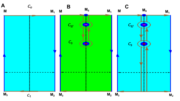
(a)    Domain of integration for the energy density

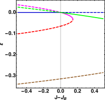
(b)    Bifurcation diagram

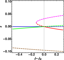
(c)    Bifurcation diagram

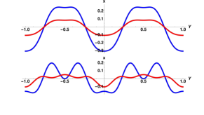
(d)     Upper interface profiles

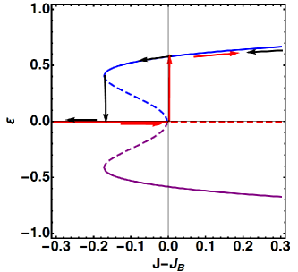
(e)    Bifurcation diagram

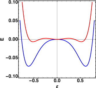
(f)     Elastic energy for $\bm{J=J_{B}\pm 0.1}$

Figure 4: Domain ${\cal P}$ for integration of the energy density, restricted to one wavelength $-1/2\leq Y\leq 1/2$, $X\in[0,+\infty]$. Only contours of interest are labeled, such as ${\cal C}_{i}$. Panel (A) is similar to panel (A) of Fig.(3), only the contour ${\cal C}_{0}$ contributes to the elastic energy, as shown in section IX.1. In (B) and (C) which is also panel (B) of Fig.(3), the relevant contours are around each singular point ${\cal S}$ and ${\cal S}_{J}$.
In panels (b) and (c), the bifurcation diagram, $\epsilon$ versus $J-J_{b}$, for a triple mode coupling with surface tension: $\gamma_{0}=0.1$. In (b), $a_{2}=0.1$ and $a_{3}=-0.1$ (curves in red and magenta) and $a_{2}=0.1$ and $a_{3}=0.1$ (curves in brown and green). Dashed curves indicate unstable solutions. In (c) $a_{2}=0.5$ and $a_{3}\pm 0.5$ with the same color code. For $a_{3}=0.5$, the stable solution appears below the Biot threshold $J_{B}$ in contrast to the other cases. In (d) interface profiles (multiplied by 10 for both axes; $J-J_{B}=0.12$ for the upper case corresponding to the data of panel (b), $J-J_{B}=-0.2$ for the lower case. In blue $a_{3}=-a_{2}$, in red $a_{3}=a_{2}$ with the exact values of $\epsilon$ chosen in each case.
In (e) a subcritical bifurcation diagram for the amplitude $\epsilon$. Continuous lines indicate locally stable solutions, dashed lines unstable solutions, not observed experimentally. Red arrows indicate the trajectory for increasing values of $J$ while black arrows indicate the trajectory for decreasing values. Note the complete symmetry between positive and negative values of $\epsilon$. The hysteresis cycle extends between the two vertical arrows indicating the jump of the $\epsilon$ amplitude at $J_{C}$ (see eq.(90)) and at $J=J_{B}$. In (f) the elastic energy density for $J=J_{B}+0.1$ in blue and $J=J_{B}-0.1$ in red as a function of $\epsilon$ with $3$ stable solutions below $J_{B}$,($3$ red minima) and only $2$ (in blue) above.

As shown in section XV.2, the surface tension creates an additive contribution in $\epsilon^{4}$ which can change the present result, giving two solutions for $\epsilon$ instead of one. An exhaustive study is really difficult due to the large number of degrees of freedom such as $a_{2}$, $a_{3}$ and $\gamma_{0}$, the dimensionless capillary number. However, this number is rather weak and for the numerical study we choose $\gamma_{0}=0.1$. The amplitude $\epsilon$ which minimizes the elastic energy is a solution of a quadratic equation, so there are two solutions in addition to $\epsilon=0$. A first numerical investigation, for coefficients $a_{2}=0.1$ and $0.5$ and $a_{3}=\pm a_{2}$ is shown in Fig.(4)(b,c) and demonstrates nonlinear modes occurring after or before the Biot threshold. Only stable solutions are considered, so only the continuous lines of Fig.(4)(b,c). From these two examples, one can notice that the $\epsilon$ values are rather weak, negative and less than $0.1$ in absolute value. The interface profiles are shown in Fig.(4)(d). At the top we find strongly distorted profiles for a value of $J=3.50$ and $\epsilon=-0.019$  ($a_{3}=-a_{2}$, $a_{2}=0.1$) and $\epsilon=-0.0065$ for $a_{3}=0.1$. Below, for $a_{2}=0.5=-a_{3}$ $\epsilon=-0.0096$ and $J=3.58$ and for $a_{3}=0.5$, $\epsilon=-0.003560$ and $J=3.18$. Fig.(4)(d) respects the scale but the height is magnified by a factor of $10$. In conclusion, this nonlinear treatment shows that nonlinear modes can occur before the Biot threshold, but for strong capillary numbers. As the amplitude of the coefficient $a_{2}$ increases, the mode becomes more and more distorted from the single sinusoidal solution but the amplitude of the interface remains small due to the small amplitude of $\epsilon$. To better understand the bifurcation plots, we choose a more appropriate representation for the profile functions in the next section.

IX.5 Super and subcritical bifurcations

In the previous paragraph, we assumed that all the coupled harmonics are of the same order of magnitude. Now, we construct profile functions where the harmonics slightly perturb the principal mode $\zeta$ such as : $\Phi(Z)=\zeta-\epsilon A_{2}\zeta^{2}(1+\alpha_{3}\zeta)$, where $A_{2}$ and $\alpha_{3}$ are constants of order $1$. In this case we get:

$${\cal E}=-{\cal Q}_{2}\delta J\pi\epsilon^{2}+\pi^{2}A_{2}{\cal Q}_{3}\epsilon^{4}\,.$$ (88)

For positive values of $A_{2}$, we recover the classical supercritical bifurcation with $\epsilon\sim\pm\sqrt{\delta J}$ above the Biot threshold. For the opposite sign of $A_{2}$ and $\alpha_{3}=-\epsilon^{2}B_{3}$ (which implies a very weak perturbation of the main mode $\zeta$), the selected profile becomes $\Phi(Z)=\zeta+\epsilon B_{2}\zeta^{2}-\epsilon^{2}B_{3}\zeta^{3}$, with $B_{2}$ and $B_{3}$ positive and in this case:

$${\cal E}=-{\cal Q}_{2}\delta J\pi\epsilon^{2}-\pi^{2}B_{2}{\cal Q}_{3}\epsilon^{4}+\pi^{2}B_{3}B_{2}{\cal Q}_{3}{\cal Q}_{33}\epsilon^{6}\,.$$ (89)

The extrema of ${\cal E}$ are obtained for $\epsilon$ values given by:

$$\epsilon(J)=\pm\frac{1}{\sqrt{3B_{3}{\cal Q}_{33}}}\left(1\pm\sqrt{1+\frac{3}{\pi}\frac{{\cal Q}_{2}}{Q_{3}}\frac{B_{3}}{B_{2}}{\cal Q}_{33}\delta J}\right)^{1/2}\,.$$ (90)

and

$$J_{C}=J_{B}-\frac{\pi}{3}\frac{B_{2}}{B_{3}}\frac{{\cal Q}_{3}}{{\cal Q}_{33}{\cal Q}_{2}}\,.$$ (91)

Fig (4) (e) and (f) show the evolution of the profile amplitude $\epsilon$ as the volumetric growth coefficient $J$ increases and decreases in the vicinity of $J_{B}$. As $J$ increases, and remains below $J_{B}$, the chosen value of $\epsilon$ remains zero (red solid curve), corresponding to the purely axial growth, but such a solution loses its stability at $J_{B}$, (red dashed curve). Then the value of $\epsilon$ makes a positive (or negative) jump $\epsilon_{G}=\sqrt{2}/\sqrt{3B_{3}{\cal Q}_{33}}$ (resp. $-\epsilon_{G}$). Then $\epsilon$ rises slightly above $J_{B}$ following the blue trajectory in the direction of the red arrow. If there is a decrease of $J$ from $J>J_{B}$, $\epsilon$ decreases along the blue line which is stable until $J=J_{C}$, where the blue trajectory loses its stability (blue dashed curve) and the flat pattern: $\epsilon=0$ is restored. At the transition there is also a jump in $\epsilon_{D}=1/\sqrt{3B_{3}{\cal Q}_{33}}$. Note that $\epsilon$ can be either positive or negative, only $\epsilon>0$ is shown for clarity but both signs are equivalent (see Fig.4)(f) which gives the energy minima for two values of $(J-J_{B})$. Only, E.Hohlfeld and Mahadevan seem to have discovered this subcritical bifurcation by numerical means (finite elements, ABAQUS), while experimentally the hysteresis associated with such a configuration was revealed by J.Yoon, J. Kim and R.C. Ryan Hayward in [77]. This scheme nicely represents the hysteresis observed in experiments. Before closing the parenthesis on nonlinear wrinkling patterns, studied with the classical techniques of bifurcation theory, let us outline a recent analysis performed with group theory methods concerning first the case of a compressed inextensible beam resting on a nonlinear foundation [43], second, the case of a thick compressed nonlinear sample [20] with different types of elasticity energy than the simple one considered here. Focusing on the first case, the very interesting point is that the authors succeed to capture localized patterns and one can wonder if it will not be possible to establish a nonlinear solitonic solution for the spatial modes detected here.

IX.6 Role of surface tension

Surface tension is a weak parameter in processes controlled by elasticity. A typical order of magnitude is given by the dimensionless number $\gamma_{0}=\gamma/\mu H$, where $\gamma$ is in Newtons per meter, the shear modulus $\mu$ is in Pascals and $H$ is a typical length, so in our case it will be the wavelength. An exact value will depend on the nature of the elastic sample and possibly of the fluid above the sample. Measurements based on elasto-capillary waves [115, 134, 135] made with extremely soft materials ($\mu\sim 100Pa$) give a value of about $0.05N/m$. Recently, the role of surface tension on creases has been considered and obviously, surface tension plays an enormous role in the vicinity of quasi-singular profiles, as naively explained by the Laplace law of capillarity [136, 137]. For small deformations, well represented by a few harmonics and for ordinary elastic materials with a shear modulus around $10^{4}$Pa, the surface tension may be relevant only in the vicinity of the bifurcation examined in the previous section IX.5. We will first consider the case where the coupling with the first harmonic $\zeta$ is weak as in section IX.5. The expansion of the energy density, eq.(89), must now include the capillary terms order by order:

$$\begin{cases}{\cal E}_{c}={\cal E}_{cs}+\frac{\gamma_{0}}{2}\left(\frac{\pi(J^{2}-1)\epsilon}{2J}\right)^{2}\\ \times\big{(}4B_{2}^{2}+B_{2}\frac{(J-1)^{2}\pi}{J})\epsilon^{2}+e_{2c}\epsilon^{4}\big{)}\,.\end{cases}$$ (92)

$E_{cs}$ is the capillary energy associated to the main mode $\zeta$. It is given by eq.(S12) and eq.(S13) while and $e_{2c}$ is given by eq.(S15), in section XV.3. $E_{cs}$ is the capillary energy associated with the main mode $\zeta$. Regarding the sign, the fourth and sixth order terms can be positive or negative so they can change the nature of the bifurcation which can go from subcritical to supercritical if $\gamma_{0}$ is strong enough. One can now examine in more detail the case where the coupling of the $3$ modes has an equivalent weight, according to the section IX.4.2. In this parameter range, the surface tension becomes a small parameter for the standard range of values of $\gamma_{0}$ and the capillarity plays a critical role at the fourth order. We rescale the free energy and rewrite the equation (78) as follows:

$${\cal E}_{t}=-E_{f}\epsilon^{2}\left(\delta J+2\gamma_{0}g_{2})+(e_{3}+2\gamma_{0}g_{3})\epsilon+2\gamma_{0}g_{4}\epsilon^{2}\right),$$ (93)

where $E_{f}$ and $e_{3}$ have been defined in eq.(78). Here we give only $g_{2}$

$$g_{2}=-\frac{\pi J(J+1)\left(1+4a_{2}^{2}+9a_{3}^{2}\right)}{(3J^{2}-6J-1)\left(1+2a_{2}^{2}+3a_{3}^{2}\right)}\,.$$ (94)

Each coefficient of the capillary energy is a function of $J$, $a_{2}$ and $a_{3}$ and is listed in section XV.3. The order of magnitude of these coefficients as $a_{2}$ and $a_{3}$ vary can be found in Fig.(8) in section XV.3. In fact, for normal values of the shear modulus, there is little chance that the capillary will alter the results given by eq.(78). Since $g_{2}$ is negative, the bifurcation threshold is shifted to higher values by capillarity. This shift depends on the representation of the profile.

Post-buckling creases were studied extensively a decade ago [29, 138, 44, 53]. These studies suggest that creases can appear before the Biot threshold due to a subcritical bifurcation, as shown here in section IX.5. Note that the numerically detected creases in these studies require the introduction of periodic defects. Cao and Hutchinson [138] demonstrate the remarkable sensitivity of wrinkling results to physical imperfections and defects. This is not surprising, since it is a general property of the bifurcation theory [33].

The case of the self-contacting interface is much more difficult to handle, since analyticity is not preserved on a line (or on a segment) in the plane, so the elasticity equations are no longer valid. If we approximate the two Heaviside distributions that mimic the self-contacting interfaces by an analytic function such as $\Phi=-b^{2}\sqrt{Z^{2}+a^{2}}$, where $a$ is a tiny quantity, there is no reason to assume real contact between the two surfaces, which will remain separated by $2a$. Thus, self-contacting interfaces are intentionally created like fractures. They can be nucleated by defects and then, they will have a better chance to be observed in thin samples, i.e.in $2$ dimensions compared to $3$ dimensions (see Dervaux’s thesis [74]). Nevertheless, such triggered singularities remain a very attractive area of study, as shown by the experiment of a deflated cavity localized at a finite distance from the upper boundary [38]. Before the generation of the self-contact, a quasi-singular profile is obtained with the scaling $x\sim|Y|^{2/3}$, which is similar to our last profile function $\Phi$ of eq.(63), on the right but with a different exponent. The curvature at the singularity varies as $|Y|^{-1/3}$ like $x^{-1/2}$. This experiment is strongly reminiscent of the equivalent one realized in viscous flow by Jeong and Moffatt [47] with contra-rotating motors. Although the interface behavior recovers the same exponent at some distance from the singularity, the curvature remains finite and parabolic at the singularity, the only unknown being the radius of curvature at the tip, which is chosen by the surface tension.
In conclusion, the observation of a bifurcation occurring before the Biot threshold is possible if at least $3$ harmonic modes are initially coupled in the nonlinear regime. For the quasi-singular profile, the answer depends too much on the mathematical description of the profile. However, here we have presented a way to fully analyze the nature of the bifurcation in the neighborhood of the Biot threshold in order to obtain valuable predictions.

X How to escape the Biot threshold?

In the previous sections, the existence of creases occurring at or just after the Biot threshold was examined. There is no difficulty in generating such creases as shown above, using the tools of complex analysis. However, it has been suggested by heuristic arguments [139, 44, 29] that singularities inside elastic samples can induce bifurcation below the threshold: $J_{B}$. Singularities induced by stresses are not forbidden in plane strain or plane stress elasticity, provided that the local elastic energy remains finite even if the energy density does not. In practice in $2D$, this means that the strains are not more singular than $R^{1/2}$ and the elastic deformation gradient or the stresses are not more singular than $R^{-1/2}$, where $R$ represents the distance to the singular point $R\rightarrow 0$. In linear plain strain elasticity, this is the case for the fracture tips and also for edge dislocations. The main difference between linear and this work is the fact that linear elasticity does not consider the nucleation of such defects that exist prior to loading and focuses more on the opening and/or the displacement of the fracture. There are very few theoretical or experimental investigations about the fracture nucleation [70, 140, 141, 142, 143, 144]. The hope here is indeed to generate these peculiar structures by volumetric growth or by compression. The main question we have to solve is the following: is it possible to lower the bifurcation threshold by considering singularities inside the sample?

As already mentioned in eq.(60), the solvability condition to observe periodic solutions implies either $J=J_{B}$ or $\Re\,[\Phi_{Z}]=0$, for $X=0$ so $\Phi$ is an even function of $Z$. Here we avoid here a singularity at the interface $X=0$, which requires a modification of the elastic model with a surface energy [45]. A nonlinear singular solution emerges, but it does not satisfy the simultaneous cancellation of normal and shear stress at $X=0$ [46]. So we focus on singularities inside the sample. An even function of $Z$, that can be represented by $\Phi(Z)=F(Z)+F(-Z)$, automatically exhibits singularities inside the sample if convergence at positive infinity is required: a holomorphic function, other than a constant, cannot converge at both infinities without singularities. The choice is then a periodic allowed singular function, eliminating poles and avoiding as much as possible extended branch cuts, always a source of stress.

X.1 Singular Profiles below the Biot threshold

In finite elasticity, such as the Neo-Hookean elasticity, allowed singularities in plane strain must induce a local finite elastic energy, which in practice means that $|F_{Z}|$ cannot be more singular than $|Z-X_{0}|^{-1/2}$, where the positive constant $X_{0}$ denotes the central position of the singularity. Larger exponents are allowed since they do not contribute locally to the total elastic energy. Existing branch-cut singularities must remain limited in size. However, singular solutions can locally invalidate the hypotheses of the initial elastic model and may require more complexity in the elastc representation and even in the growth process. As an example, in fast fracture dynamics [145, 146, 147], $3$ possible zones for the crack tip have been identified: first the viscoelastic, then the nonlinear elastic, and finally the traditional linear-elastic zone, which produces the square root singularity [148]. Of course, such a description requires different physical models at different length scales. Whatever the complexity introduced into the modeling, such as multiple invariants of finite elasticity, compressibility, plasticity or strain hardening, and eventually growth variations, it must remain localized in a small domain and must be treated as an inner boundary layer. Let us fix this domain around $X_{0}$ and choose $\Phi$ as:

$$\Phi(Z)=F(Z-X_{0})+F(-Z-X_{0})\,,$$ (95)

where $F(Z)=\bar{F}(Z)$. The function $F$ is periodic with period one, real or its Laurent series has only real coefficients and is convergent for $Z\rightarrow\infty$. Calculating the derivative of $\Phi$ for $Z=IY$, it is easy to see that $\Re\,[\Phi_{Z}]=0$ so the normal stress $S_{11}$ vanishes and there is no need to cancel ${\cal Q}(J)$, see Eqs.(58,59,60). For $F$, two square root singularities are chosen, located at $X_{0}\pm l_{0}$ and separated by a branch cut. For symmetry reasons, we will fix the branch cut along the $X$ axis as follows:

$$F_{Z}=\frac{1}{\sqrt{\tanh^{2}(\pi Z)-\tanh^{2}(\pi l_{0})}}-\cosh(\pi l_{0})\,.$$ (96)

The last term fixes the cancellation of $F_{Z}$ when $Z\rightarrow\infty$. $l_{0}$ is a tiny parameter that specifies the size of the branch cut $2l_{0}$. Useful for the following, $F(Z)$ is the primitive function of eq.(96):

$$F(Z)=f(Z)-Z\cosh(\pi l_{0})\,,$$ (97)

where

$$f(Z)=\sqrt{\frac{\sinh^{2}(\pi Z)-\sinh^{2}(\pi l_{0})}{\tanh^{2}(\pi Z)-\tanh^{2}(\pi l_{0})}}\frac{h(Z)}{\pi\cosh(\pi Z)}\,,$$ (98)

and

$$h(Z)=\tanh^{-1}\left(\frac{\sinh(\pi Z)}{\sqrt{\sinh^{2}(\pi Z)-\sinh^{2}(\pi l_{0})}}\right)\,.$$ (99)

Several observations must be made at this stage:

• The choice of $F_{Z}$ is somewhat arbitrary, but takes into account symmetry arguments and is also dictated by its simplicity.

• Less singular functions with the square root replaced by a power law $(w)^{1/2}\rightarrow(w)^{a}$, where $a>1/2$, are also possible a priori.

• As soon as we introduce a singular zone around $X_{0}$, this automatically produces another singularity around $X_{0}/J$ which will influence the interface more strongly, at $X=0$. So we are faced with two boundary layers which are easier to treat independently. So $J>1$ and $l_{0}<<<1$.

• When introducing such profiles, we are faced with a minimal list of parameters such as $l_{0}$, $X_{0}$, $\epsilon$ and $J$. We hope to find $J$ below the Biot threshold $J_{B}$ and to find constraints on these parameters. These parameters must be fixed in a consistent way.

• Finally, such localized singularities are often found in periodic viscous flows where the equivalent of our ”blob” is the bubble in the viscous flow [149, 120, 119, 58]. Note that in the case of bubbles, there are several families of solutions that depend on the bubble location and its symmetries.

The contribution of such a function $F(Z)$ on the interface and on the stress accumulated inside the sample are shown in Fig.(5). In order to show that such a scenario can exit, it is necessary to establish the existence of semi-singular patches where the stresses are concentrated. it will also be necessary to relate the four parameters $l_{0}$, $X_{0}$, $\epsilon$ and $J$ to other physical processes occurring in the inner boundary layer which are neglected in the outer zone.

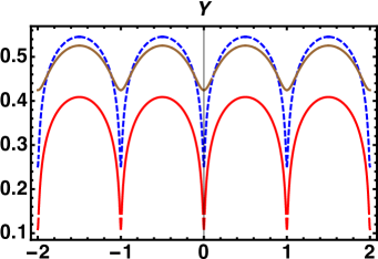
(a)  Interface profiles

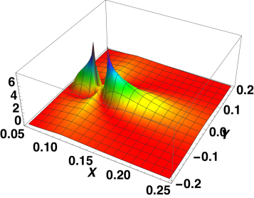
(b)   Singularities of $\bm{S_{11}}$

Figure 5: On the left, profiles corresponding to the deformation given by eq.(98). The parameters are $J=3,\epsilon=0.1$. For the blue profile $X_{0}=0.01$ and $l_{0}=0.001$, for the red curve, the same $X_{0}$ value and $l_{0}=0.005$, for the brown profile, $l_{0}=0.001$ and $X_{0}=0.1$. Note that $l_{0}$ has little effect on the shape profile, which depends strongly on the distance of $X_{0}$ from $X=0$. The difference in height of the averaged surface has no physical meaning. On the right, the stress $S_{11}$ in logarithmic scale ($Log(1+S_{11}^{2}$), multiplied by a scaling factor of $0.01$ for visualization purposes, with $l_{0}=0.01$ and $X_{0}=0.1$. Note the two singular zones around $X_{0}$ and $X_{0}/J$. These singularities will merge in the boundary layer. The stress decreases rapidly so that the map is confined to a limited area of the sample between $0.0<X<0.25$ and $-0.2<Y<0.2$.

X.2 Physical origins of the patches

Several origins can explain the existence of patches, sites of focusing of the elastic stress. Such focusing locally destroys the linear expansion of the elastic deformation in $\epsilon$ , making the validity of the linear expansion questionable. But also, at large strains, it can invalidate the model itself: the choice of the neo-Hookean elastic energy, the incompressibility hypothesis, the constant volumetric growth. Let us examine each of these possible causes:

• The neo-Hookean model, very convenient for its simplicity fails to describe a focusing, either too strong or too localized and must be corrected by a more sophisticated hyperelasticity model involving nonlinearities in $I_{1}$ or other invariant such as $I_{2}$.

• The incompressibility limit is a mathematical limit that is not appropriate for large strains. A more physically relevant model may be a quasi-incompressible approximation with a strong coefficient multiplying the invariant $I_{3}$ in the elastic energy [44].

• Spatially constant volumetric growth is a naive approximation of a true biological process. In fact, for growing living species, an excess of compressible stress is known to inhibit the cell proliferation. It is reported as the principle of homeostasis [150].

• This phenomenon also occurs in swelling. Everyone knows how to expel water from a wet sponge, simply by applying a pressure to it.

The complete solution of the nonlinearities is hopeless, since it is impossible to find a nonlinear solution inside the patch that asymptotically recovers the expansion given by Eqs.(96,98). But, we know similar situations in solid mechanics where nonlinearities play an essential role in a localized region around a singular point, as in fracture mechanics or dislocation theory, and are responsible for a constant stress intensity factor. As shown by Barenblatt [151, 152], w these nonlinearities, if they remain localized, do not prevent the validity of the linear theory, except in the zones of high predicted stress where they soften. In the next section, we relax some of the limitations of the model, by adding nonlinearities and compressibility, while keeping the volume growth constant.

X.3 Patches as inner boundary layer

In the first patch located at $Z=X_{0}$, a new coordinate $U$ such as $Z-X_{0}=\frac{1}{\pi}\tanh^{-1}(\tanh(\pi l_{0})U)$ gives the following expansion of eq.(98) in the limit of small $l_{0}$

$$F(Z)\sim\frac{1}{2\pi}\left\{Log\left(\frac{U+\sqrt{U^{2}-1}}{-U+\sqrt{U^{2}-1}}\right)+\phi_{0}\right\}\,,$$ (100)

and $\quad x\sim JX+\epsilon J(\Re\,[F(Z)]+x_{1})$ with $x_{1}=\Re\,[\phi_{0}+F(-X_{0})+J\tau_{1}\Re\,(F((J-1)X_{0})+F(-(J+1)X_{1})]$. This expansion shows that $F(Z)$ has two singular points $U\pm 1$ separated by a branch cut. For $|Z-X_{0}|>l_{0}$, then $U>1$, so $l_{0}<Z-X_{0}<1$, the asymptotic behavior of $F(Z)$ is logarithmic, which gives for the outer profile:

$$\begin{cases}x&\sim JX+\epsilon\left\{\frac{J}{2\pi}Log\left(\frac{(X-X_{0})^{2}+Y^{2}}{l_{0}^{2}}\right)+x_{1}\right\}\,,\\ y&\sim Y-\frac{\epsilon}{\pi}\tan^{-1}\frac{Y}{X-X_{0}}\,.\end{cases}$$ (101)

For the second patch ${\cal S_{J}}$ located at $X_{0}/J$, a similar expansion for $Z_{1}$ with the definition of $U_{1}=JU_{X}+IU_{Y}$ gives a similar result, the only difference being the expansion of coordinates $(x,y)$:

$$\begin{cases}x&\sim JX+\frac{\epsilon J\tau_{1}}{2\pi}\left\{Log\left(\frac{(JX-X_{0})^{2}+Y^{2})}{l_{0}^{2}}\right)+x_{2}\right\}\,,\\ y&\sim Y-\frac{J\epsilon\tau_{1}}{\pi}\tan^{-1}\frac{Y}{JX-X_{0}}\,.\end{cases}$$ (102)

The fact that we have two independent small parameters ( $\epsilon$ and $l_{0}$ ) suggests a complicated double boundary layer. An example is also given by fracture mechanics, where a separation of length scales is necessary and has been estimated in [148, 153]. Indeed, in soft and highly deformable materials, we cannot neglect nonlinear deformations and the dissipation for fast dynamics even if Hookean elasticity gives a reasonable picture of cracks. The separation of length scales, in [148] includes the inner scale (the crack tip) due to a large amount of dissipation, the intermediate scale due to the nonlinearities of elasticity and finally the outer scale where linear elasticity is allowed. Again, two different length scales: $\zeta$ for dissipation and $l$ for nonlinearities coexist and have been experimentally verified [148]. In our case, we can disregard dissipation since either growth or gel swelling are slow processes, see Fig.(1)(A8,A9) and [74]. However, as with fractures, additional physical properties are needed in order to fulfill the neo-Hookean model with incompressibility which has an inherent lack of parameters and length scales. In the next section, we extend the neo-Hookean model by incorporating nonlinearities in the elastic energy such as $I_{1}^{2}$ and $I_{2}$ and also the third invariant $I_{3}$, which is responsible for the compressibility.

XI Theoretical evidence for internal singularities

XI.1 New elastic model for large stresses

We start by locally assuming a more complex elastic energy and we focus on the patches located around $X_{0}$ and $X_{0}/J$. They are separated by a distance $X_{0}(J-1)/J\sim 2/3X_{0}$. We assume two boundary layers around each patch: an inner zone of size $l_{0}$ and an outer zone of size $l_{p}$ such that $l_{0}<l_{p}<<X_{0}$, to avoid overlapping between the two patches. The existence of two boundary layers is required, first, to eliminate the square root singularity and, second, the necessity to recover the logarithmic asymptotic before the linear expansion in $\Phi(Z)$. Besides nonlinearities in the modeling of the hyperelasticity density, the limit of complete incompressibility can be questionable when the strains become very large. There are a significant number of models in the literature that treat compressibility, see chapters $6$ and $8$ of [91]. Due to the large strains localized in the patches, the best approach is the compressible model of R. Ogden [93, 91], which separates the elastic energy density into two parts: $\Psi_{iso}$ and a volumetric part, also called the bulk part $\Psi_{vol}$. In practice however, it is very difficult to find explicit solutions that occur on a scale smaller than $l_{0}$. So we focus first on the intermediate regime where $|Z-X_{0}|>l_{0}$ and we restrict on nonlinearities in $I_{1}$ and a compressibility penalty treated as a quadratic expansion. For the elastic energy density: either $\Psi^{(p)}$ (nonlinear model) or $\Psi^{(mr)}$ (the Mooney-Rivlin model) the following expressions are given for geometric invariants which are corrected by the growth according to eq.(44):

$$\begin{cases}\Psi^{(p)}&=\tilde{I}_{1}+\frac{\omega_{p}}{J^{2p-1}}\tilde{I}_{1}^{2p}+\frac{\kappa}{J}(\tilde{I}_{3}-J)^{2}\\ \Psi^{(mr)}&=\tilde{I}_{1}+\frac{\omega_{mr}}{J}\tilde{I}_{2}+\frac{\kappa}{J}(\tilde{I}_{3}-J)^{2}\,,\end{cases}$$ (103)

where $p$ is a real number greater than $1$, $\omega_{p}$ and $\omega_{mr}$ are small parameters, positive or negative, representing a first correction to the neo-Hookean elasticity, but $\kappa$ is expected to be a large positive quantity to mimic the quasi-incompressibility.

XI.2 The intermediate boundary layer analysis

For the first patch, we define the rescaled quantities for the space coordinates in the initial configuration:

$$\hat{X}=(X-X_{0})/l_{p};\quad\hat{Y}=Y/l_{p}\,.$$ (104)

A localized patch ${\cal S}$ or ${\cal S}_{J}$ requires $l_{p}\leq X_{0}$ and to recover the asymptotics of $F(Z)$, we assume a solution for the profile function $\epsilon(x_{s}(\hat{R}),\epsilon y_{s})$ given by:

$$x_{s}=\frac{\epsilon}{\pi}f_{s}(\hat{R})+JX_{0}\quad{\mbox{and}}\quad y_{s}\sim\frac{-\epsilon}{\pi}T\,,$$ (105)

where $\hat{R}=\sqrt{\hat{X}^{2}+\hat{Y}^{2}}$ and $T=\arctan(\hat{Y}/\hat{X})$. Assuming a possible correspondence with eq.(101), the unknown function $f_{s}$ must satisfy $f_{s}(\hat{R})\sim JLog\hat{R}$, for large values of $\hat{R}$, but must remain finite for small values of $\hat{R}$, a property which is not verified by eq.(101). This gives the following scaling for the invariants:

$$\tilde{I}_{1}=\epsilon^{2}/(\pi l_{p})^{2}\,,\quad\tilde{I}_{1}^{p}\sim\epsilon^{4p}/(\pi l_{p})^{4p}\,,\quad\tilde{I}_{3}\sim\epsilon^{2}/(\pi l_{p})^{2}.$$ (106)

The size of the boundary layer given by $l_{p}$ must eliminate arbitrary coefficients as much as possible. Note that $l_{p}$ is a tiny value, unlike $\kappa$ which can take large values to represent quasi-incompressible material. Define:

$$\begin{cases}\tilde{I}_{1}=\frac{\epsilon^{2}}{\pi^{2}l_{p}^{2}}\hat{I}_{1};\quad\hat{I}_{1}=\frac{1}{\hat{R}^{2}}+f_{s}^{\prime}(\hat{R})^{2},\\ \tilde{I}_{3}-J=-J\hat{K};\quad\hat{K}=1+|\omega_{p}|^{-1/p_{0}}\frac{f_{s}^{\prime}(\hat{R})}{\hat{R}},\end{cases}$$ (107)

where $p_{0}=2p-1$ and $l_{p}=|\epsilon|/\pi|\omega_{p}|^{1/(2p_{0})}J^{-1/2}$, then the elastic energy, for the new elasticity model given by eq.(103), is transformed to :

$${\cal E}_{s}=\frac{\epsilon^{2}}{\pi}\int_{0}^{\infty}\hat{R}d\hat{R}\left(\hat{I}_{1}+\hat{I}_{1}^{2p}+J\kappa\hat{K}^{2}\right).$$ (108)

Variation with respect to $f_{s}$ leads to a second order E-L equation, which can be integrated once without difficulty, and finally we are faced with a first order nonlinear differential equation:

$$\hat{R}f_{s}^{\prime}(\hat{R})\left(1+2p\left(f_{s}^{\prime}(\hat{R})^{2}+\frac{1}{\hat{R}^{2}}\right)^{p_{0}}\right)\\ +\kappa_{0}\frac{f_{s}^{\prime}(\hat{R})}{\hat{R}}=C_{S},$$ (109)

where $\kappa_{0}=J\kappa\,|\omega_{p}|^{-1/p_{0}}$ and $p\geq 1$. $C_{s}$ is an arbitrary integration constant at this stage. In the quadratic case, $p=p_{0}=1$, the Euler-Lagrange equation for $\hat{x}_{s}$ is easily solved, and the second Euler-Lagrange equation for $\hat{y}$ is automatically satisfied once the relation eq.(105) is imposed. Even if an exact solution can be found, we focus on the two limits of interest, first for $\hat{R}\rightarrow 0$ and then for $\hat{R}\rightarrow\infty$:

$${\mbox{For}}\quad\hat{R}\rightarrow 0\quad f^{\prime}_{s}(\hat{R})=\frac{Cs\hat{R}^{4p-3}}{2p+\kappa_{0}\hat{R}^{4(p-1)}}\,.$$ (110)

Regardless of the value of $p\geq 1$, the behavior of $f_{s}$ is a regular function of $\hat{R}$, as it is required for a physical solution. Note that $\kappa_{0}$ only plays a critical role if $p=1$, which leads to:

$${\mbox{For}}\quad\hat{R}\rightarrow 0\quad f^{\prime}_{s}(\hat{R})=\frac{C_{S}}{2p+\kappa_{0}}\hat{R}\,.$$ (111)

Finally, choosing $C_{s}=J$ leads to the convenient asymptotic for $f_{s}$ when $\hat{R}\rightarrow\infty$ whatever the $p$ values. So the outer boundary layer seems to satisfy the physical requirements, see eq.(101). Since we have introduced two boundary layers: an inner core of size $l_{0}$ and an intermediate zone of size $l_{p}>l_{0}$, this allows to easily perform the adjustment in the asymptotics of $F(Z)$ given by eq.(100). Another standard way to modify the neo-Hookean model is the Mooney-Rivlin model, which is even simpler:

$$\hat{R}\left(\frac{df_{s}}{d\hat{R}}\right)\left(1+\frac{1}{\hat{R}^{2}}\right)=-\frac{\kappa_{mr}}{\hat{R}}\left(\frac{df_{s}}{d\hat{R}}\right)+C_{s}\,,$$ (112)

with $\kappa_{mr}=J\kappa/\omega_{mr}$ and $l_{mr}=\epsilon/\pi\sqrt{\omega_{mr}/J}$. The solution for $f_{s}$ is easily found and in physical units, we have:

$$x_{s}=\frac{J\epsilon}{2\pi}Log\left\{\frac{R^{2}}{l_{mr}^{2}}+\left(1+\frac{\kappa_{mr}}{\omega_{mr}}\right)\right\}\,,$$ (113)

with no change for $y_{s}=-\epsilon T/\pi$.
However, in the inner region very close to $X_{0}$ where $|Z-X_{0}|\leq l_{0}$, these solutions given by eq.(110,112) present a singularity of the strain in $1/R$ due to the choice of $y_{s}$, which limits their validity in this inner zone.
Note that, for both models, $x_{s}$ has the same asymptotic limit for $R>\it{l}_{p}$ and they are regular for $R->0$, so even if we are not able to find the inner core solution, we can recover the result of eq.(101) and the correct asymptotic of $\Phi(Z)$.

The same analysis applies to the upper singularity centered around $X_{0}/J$. For the second patch ${\cal S_{J}}$, the same strategy is followed, and it is easy to show that the associated deformations $(\hat{x}_{S_{J}},\hat{y}_{S_{J}})$ according to eq.(102) satisfy :

$$\begin{cases}\hat{x}_{s_{J}}=\frac{1}{2\pi}Log\left(\frac{1}{\pi^{2}}+J^{2}\hat{X}^{2}+\hat{Y}^{2}\right)\\ {\mbox{and}}\\ \hat{y}_{s_{J}}=-\frac{1}{\pi}\tan^{-1}\frac{\hat{Y}}{J\hat{X}}\,.\end{cases}$$ (114)

The same matching between deformations in the second patch is done by $\epsilon\tau_{1}(Jx_{s_{J}},y_{s_{J}})$ which gives the same analysis for both patches. So, both singularities can be treated in the same way.

In summary, once linearized, the primary incompressible model can have two patches ${\cal S}$ and ${\cal S}_{J}$ with a singularity inside. The actual patch size is $l_{p}$. Each patch contains an inner core of size $l_{0}^{p}$ and an intermediate zone of size $l_{p}$, corresponding to two boundary layers with a more regular stress distribution. The main information we obtain for the treatment of the intermediate zone is in fact its size $l_{p}$ given by $\epsilon$ and the first nonlinear correction of the neo-Hookean energy scaled by the constant: $|\omega_{p}|$.

XI.3 The inner core

In the inner core, the strains and stresses are expected to increase again, and perhaps the specimen is strongly modified by nonlinearities going from stress hardening to plasticity [154] Such material transformations have been studied in detail in the fracture mechanics literature [147, 148]. Here we try to stay as close as possible to our original model although we agree that any modification of the material structure is possible and may change some conclusions. Therefore, we keep the compressible hyperelasticity point of view but we reinforce the compressibility analysis of the material with the Ogden model, where the elastic energy is decoupled into a purely volumetric elastic response and a dilatational part [93]. As explained in section III.2 at the very beginning of the paper, this requires a new definition of the strains according to eq.(5).

XI.3.1 Rescaling the strains and the invariants

We retain the quadratic compressibility model of the previous paragraph, which is still a function of $I_{3}$ although other approximations may be more appropriate for $R\sim l_{0}^{p}$ (see Chapter $6.5$ of [91]). Within the inner core, we suggest the following description for the current coordinates $(x_{c},y_{c})$:

$$x_{c}=\frac{\epsilon}{\pi}l_{0}^{s}\bar{F}(\rho,\theta);\,\,y_{c}=-\frac{\epsilon l_{0}^{q}}{\pi}\bar{G}(\rho,\theta)\,.\\$$ (115)

with $\rho=R/l_{0}^{p}$ and $\theta=T/l_{0}^{q}$. We restrict ourselves to a cubic nonlinearity $I_{1}^{3}$ for reason of simplicity but the method can be applied to any kind of dilatational hyperelasticity. We impose that $p$ and $q$ are positive and that $x_{c}$ and $y_{c}$ are regular for $\rho\rightarrow 0$. For $\rho\rightarrow\infty$, the matched asymptotic analysis required that $x_{c}$ and $y_{c}$ coincide with the behavior of $x_{s}$ and $y_{s}$ for $R\rightarrow 0$. For $y_{c}$, this simply requires $G\rightarrow-\theta$. For $x_{c}$, we first consider $x_{s}$ from eq.(111), in the neighborhood of $R\rightarrow 0$:

$$x_{s}=\frac{\epsilon J}{\pi}\frac{R^{2}}{6\,l_{3/2}^{2}}\quad\mbox{where}\quad l_{3/2}=\frac{\epsilon}{\pi\sqrt{J}}|\omega_{3/2}|^{1/4}.$$ (116)

Thus, at infinity, $x_{c}$ must behave as $x_{c}\sim\rho^{2}$ and matching with $x_{s}$ gives a more precise result:

$$x_{c}=\frac{\epsilon}{\pi}l_{0}^{s-2p}R^{2}\,\Rightarrow\,l_{0}=\left(\frac{6\,l_{3/2}^{2}}{J}\right)^{1/(2p-s)}.$$ (117)

If these conditions are satisfied, the inner coordinates $(x_{c},y_{c})$ can correctly match the corresponding ones $(x_{s},y_{s})$ in the intermediate zone, allowing to recover eq.(114). However, our analysis involves many degrees of freedom in addition to the unknown material parameters $\kappa$ and $\omega_{3/2}$. Most likely, there will be several possibilities and to limit them, we recapitulate the different constraints. Since the singularity of the strains calculated with $x_{s}$ and $y_{s}$ comes from the derivative with respect to $T$, we impose that the corresponding strains for $x_{c}$ and $y_{c}$ dominate. After evaluating the amplitude of the strains, we get:

$$\begin{cases}\frac{\partial x_{c}}{\partial R}&=\frac{\epsilon}{\pi}l_{0}^{s-p}\frac{\partial\bar{F}}{\partial\rho}<<\frac{1}{R}\frac{\partial x_{c}}{\partial T}\sim\frac{\epsilon}{\pi}l_{0}^{s-p-q}\frac{1}{\rho}\frac{\partial\bar{F}}{\partial\theta},\\ \\ \frac{\partial y_{c}}{\partial R}&=-\frac{\epsilon l_{0}^{q-p}}{\pi}\frac{\partial\bar{G}}{\partial\rho}<<\frac{1}{R}\frac{\partial y_{c}}{\partial T}\sim-\frac{\epsilon}{\pi\rho}l_{0}^{-p}\frac{\partial\bar{G}}{\partial\theta}\,.\end{cases}$$ (118)

$\frac{\partial\bar{F}}{\partial\rho},\,\,\frac{\partial\bar{F}}{\partial\theta},\,\,\frac{\partial\bar{G}}{\partial\rho},\,\,\frac{\partial\bar{G}}{\partial\theta}$ being quantities of order one, then the exponent $q$ is positive. Now we examine $I_{1}$, reduced to the shear strains:

$$I_{1}\simeq\frac{\epsilon^{2}}{\pi^{2}}l_{0}^{-2p}\frac{1}{\rho^{2}}\left(l_{0}^{2(s-q)}\left(\frac{\partial\bar{F}}{\partial\theta}\right)^{2}+\left(\frac{\partial\bar{G}}{\partial\theta}\right)^{2}\right).$$ (119)

The two terms in $I_{1}$ are of different weight. However, only the first one gives the correct asymptotics for the Euler-Lagrange equations, such as $x_{c}\sim\rho^{2}$. This imposes $s<q$. Then we define $\hat{I}_{1}$ and $\hat{I}_{3}$

$$\begin{cases}I_{1}=\frac{\epsilon^{2}}{\pi^{2}}l_{0}^{2(s-q-p)}\hat{I}_{1},\quad I_{3}=\frac{\epsilon^{2}}{\pi^{2}}l_{0}^{s-2p}\hat{I}_{3},\\ \hat{I}_{1}=\frac{1}{\rho^{2}}\left(\frac{\partial\bar{F}}{\partial\theta}\right)^{2},\\ \hat{I}_{3}=\frac{1}{\rho^{2}}\left(\frac{\partial\bar{F}}{\partial\rho}\frac{\partial\bar{G}}{\partial\theta}-\frac{\partial\bar{F}}{\partial\theta}\frac{\partial\bar{G}}{\partial\rho}\right).\end{cases}$$ (120)

XI.3.2 The energy density of the inner core

Although families of possible deformations have been published for arbitrary elastic energy densities, very few concern compressible materials ([155, 156, 157]). Since we can expect a high compression in the inner core, we modify the bulk energy and adopt the Ogden model [93, 91] of compressible constrained materials, but keep the penalty term as before. There are then two choices, depending on the value of $\vartheta=|\omega_{3/2}|l_{0}^{2s-4q}/J^{2}$. In fact $|\omega_{3/2}|$ is a tiny amount, but $s<q$ so $\vartheta$ is arbitrary.

• $\vartheta<<1$, defining $K_{1}=\frac{\kappa}{J}\frac{\epsilon^{4}}{\pi^{4}}l_{0}^{s-4p+2q}$

  $$W_{c}=l_{0}^{s-2q}\left(\frac{\hat{I}_{1}}{\hat{I}_{3}}+K_{1}\hat{I}_{3}^{2}\right).$$ (121)

• $\vartheta>>1$, and $K_{2}=\frac{J\kappa}{|\omega_{3/2}|}\frac{\epsilon^{4}}{\pi^{4}}l_{0}^{6q-4p-s}$

  $$W_{c}=\frac{l_{0}^{3s-6q}|\omega_{3/2}|}{J^{2}}\left(\pm\left(\frac{\hat{I}_{1}}{\hat{I}_{3}}\right)^{3}+K_{2}\hat{I}_{3}^{2}\right).$$ (122)

A good way to get very low values of $l_{0}$ is to choose $p\simeq s/2$. However, it is sufficient to have $2p<2+s$. In addition, one must reduce the elastic energy which is confined in the core.This means that $2q-s$ must be as small as possible. In this context, the elastic energy trapped in the core can be estimated to be around $l_{0}^{s-2q+2p}$, which means that $s-2q+2p>0$ must be positive for the first hypothesis, and for the second, a necessary condition is $3s-6q+2p>0$. It is relatively easy to choose good parameters, such as $s=0,p>q$ or $s=0,p>3/2q$ for the second choice. However, these conditions may not be sufficient and must be compared with the elastic energy in the intermediate range. Note that the nonlinear eigenvalues $K_{1}$ and $K_{2}$ are numbers that are difficult to predict even as an order of magnitude. Whatever the hypothesis, eq.(121) or eq.(122), the corresponding asymptotics perfectly check the overlap with $x_{s}$ and $y_{s}$ for $\rho\rightarrow\infty$, and the behavior for $\rho\rightarrow 0$, for eq.(121) is $\bar{F}(\rho,\theta)\sim\rho$ and the same for $\bar{G}$. The analysis for the second hypothesis is less obvious. This study proves that the matching is possible and the deformation remains regular, but due to the degrees of freedom as $p$ and $q$, we do not get any information about $J$ and $\epsilon$, $X_{0}$ and $l_{0}$ as a function of the material parameters $\kappa$ and $\omega_{3/2}$. At this stage, it remains to evaluate how the zero order elastic energy is modified by the localized compression zones. In fact, a bifurcation is possible if the elastic energy is reduced.

XI.4 Energy of the patches

The goal now is to evaluate the elastic energy involving the entire physical plane (the zero-order and linear expansion in $\epsilon$) and the energy due to the patches, including the inner core and the outer ring of both singular patches. As shown before, in section IX, the expansion of the elastic field has $3$ contributions in power of $|\epsilon|$, see eq.(69). If there are no singularities inside the physical plane, the linear term ${\cal E}_{1}$ vanishes. If there are singularities, this is not the case and one has to evaluate this term. For this, we use the same method of complex analysis as described in IX.1:

$$\begin{cases}{\cal E}_{1}&=\tau_{0}\iint_{\cal P}dS\Re\,[\Phi_{Z}+J\tau_{1}\Phi_{Z_{1}}]\\ &=\frac{\tau_{0}^{2}}{2J^{2}}\Re\,[\frac{1}{2I}\iint_{\cal P}dZd\bar{Z}\Phi_{Z}]\end{cases}$$ (123)

Without singularities inside the physical plane, the integration contour called ${\cal\partial P}$, which can be observed in Fig.(4), first row on the left, corresponds to the outer boundary of the physical strip and because of the periodicity of $\Phi$ the integration gives no contribution. This is not the case now since the calculation requires to cross the cell in the middle along paths that go from the point $M_{0}$ up to the first and second singularities ${\cal S}$ and ${\cal S}_{J}$ and up along the neighboring path on the right (see Fig.(4, first row)). So the additive contribution comes from the two circular contours around the singularities. After simple simplifications and taking the size of the singularity radius as $l_{S}\sim l_{1}$, for both patches, we get:

$$\begin{cases}{\cal E}_{1}&=\frac{\tau_{0}^{2}}{2J^{2}}\Re\,[\frac{1}{2I}\oint_{\cal\partial P}dZ\Phi(\bar{Z})\\ &=\frac{\tau_{0}^{2}}{4J}\frac{l_{s}}{\pi}\Re\,\,[\int_{-\pi}^{\pi}dTe^{IT}(-IT)]=\frac{\tau_{0}^{2}}{2J}l_{1}\,.\end{cases}$$ (124)

Thus, the singularities inside the sample give a correction of the elastic energy of order $\epsilon l_{1}$ which, if $\epsilon<0$, indicates a possible bifurcation: for negative $\epsilon$, the singular solution is less energetic than the uniform axial growth. However, one must also evaluate the energy inside the core of the patches, for both singularities. Evaluating the energy inside the inner core in each singular patch leads to :

$${\cal E}_{c}\simeq|\omega_{3/2}|l_{3/2}^{\varpi};\quad\varpi=\frac{2}{2p-s}(3s-6q+2p).$$ (125)

where $\varpi=p(3s-6q+2p)/(2p-s)$. In order to compare with the energy of the intermediate zone, $\varpi$ must be as large as possible. Unfortunately the value $s=2p$ is not compatible with our constraints but $s=0$, $q$ small and $p=1$ leads to $\varpi\simeq 2$ which is enough for ${\cal E}_{c}$ to be negligible. This quantity has to be compared with $\epsilon l_{3/2}=\epsilon^{2}|\omega_{3/2}|^{1/4}/\pi$. Also the small amount $|\omega_{3/2}|^{1/4}>|\omega_{3/2}|$ justifies the fact that the intermediate singular zone dominates. We conclude that the dominant energy density corresponds to the uniform axial growth corrected by:

$$\delta{\cal E}\sim\epsilon\frac{(J^{2}-1)^{2}}{2J}|\epsilon||\omega_{3/2}|^{1/4}\,.$$ (126)

Thus, singularities inside the sample lower the instability threshold and are at the origin of a bifurcation. At this stage, there is no restriction on the values of $J$ except that the distance between the two singularities must be greater than $2l_{1}<X_{0}(J-1)/J$, which means that $\delta J=J-1$ must be larger than $2Jl_{1}/X_{0}$. This is a necessary condition for our analysis based on the separation of the two patches. Thus, the new bifurcation threshold results from controlled deviations from the neo-Hookean model.

XII Path independent contour integrals

A fancy and easy way to determine unknown parameters in singular elasto-static fields is to use path-independent integrals [158, 159, 160]. They result from Noether’s first theorem [161] as recently demonstrated and recalled by J. Rice and collaborators [162]. This theoretical method relates the geometric parameters of the singularities to the boundary conditions imposed on the far-field elasticity. It has been successfully applied to many topics of elasticity [163], but also to other physical fields as soon as they are governed by variational principles. One can think of interfacial potential flows (Darcy or Euler flows, [164])and electrostatic fields ([165], [162]). It is widely used in all aspects of solid mechanics such as fracture [166], dislocations. [167, 168, 169], notches [160], erosion [170], it is not limited to time-independent formulations [171], nor to linear elasticity although the finite elasticity singularity must be treated with care [168], especially in the case of non-quadratic formulations. Nonlinear problems, sometimes time-dependent, are often interpreted in terms of internal forces acting on defects present in materials and path-independent integrals have also been established in these cases [172, 166]. It remains, however, that some applications in nonlinear elasticity have been questioned [173, 174], more precisely for the so-called M integrals. Proofs of the application of this technique are justified in the Appendix section XV.6. Our goal is to to discover relationships between $l_{0}$ and $X_{0}$ and the neo-Hookean parameters with growth such as $\epsilon$ and $J$.

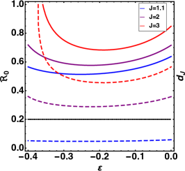
(a)   $\bm{{\cal R}_{0}=X_{0}/|\epsilon}|$ versus $\bm{\epsilon}$

(b)   Corrected values of $\bm{{\cal R}_{0}}$

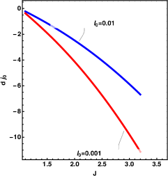
(c)   Growth difference from bottom to top

Figure 6: Panel (a) Continuous lines: the ratio ${\cal R}_{0}$ between $X_{0}$ and $|\epsilon|$ for different values of $J$, dashed lines: $d_{j}={\cal R}_{0}(J-1)/J$ the distance (divided by $|\epsilon|$) between $S_{J}$ and $S$, which must be greater than $2l_{1}/|\epsilon|=2\sqrt{|\omega_{1}|}$ represented by the dot-dashed curve in black. Panel (b) continuous lines: ${\cal R}_{0}$,dotted and dot-dashed lines, corrected values due to change of $J$ at large distances: $j_{0}\pm 0.1$, with dot-dashed lines for $+$ and dotted lines for $-$, see eq.(136).
In (c) the quantity $j_{0}d$ (jump of the growth values between the bottom and the top of the strip the times the thickness $d$ of the sample) as a function of $J$ required for two sizes of the singularity, $l_{0}=0.01$, and $l_{0}=0.001$.

XII.1 The J-Integral

This approach is not fully nonlinear because we perform an incremental expansion. In addition, our sample is pre-streched by growth which destroys the spatial isotropy. Thus, we cannot claim that the J-integral methods are directly applicable. Knowles and Sternberg have demonstrated the validity of the $J$ integral in fully nonlinear elasticity and also for incremental deformations but only when the initial state is stress-free, which is a different case. Therefore, it is important to verify that the J-integral remains valid for the model described in section VII.2. This is done in Appendix (XV.6) and we define ${\cal J}$ which is a contour integral, see Fig. (4), panel (B) or (C) above:

$${\cal J}=\oint dS(E{\bf}.{\vec{\bf e}_{x}}-N_{k}S_{ik}F_{i1})=0\,.$$ (127)

The stress $S_{ik}$ was introduced in the section VII.2, eq.(50) and eq.(53) and the strains are simply given by $F_{ij}=\partial_{j}x_{i}$. Note that the J-integral is a vector so ${\cal J}$ is only one component. Not all of the J-component can give pertinent information. The contour, shown in Fig.(4), panel B on top, first goes from $M$ to $M_{0}$, the center of ${\cal C}_{0}$, then it goes down to avoid the two singularities ${\cal S}_{J}$ and ${\cal S}$, it climbs up to $M_{0}$ to join the point $M_{1}$, it continues along $M_{1}M_{2}$, then $M_{2}M_{3}$ and finally $M_{3}M$. Only the brown paths can contribute, the blue paths cancel each other out for reasons of periodicity and symmetry. Focusing on the contour ${\cal C}_{0}$, which is $MM_{1}$ at the top of the domain, only the energy density contributes, since both normal stress components vanish, a necessary condition for a free boundary. Decomposing ${\cal J}$ into ${\cal J}^{(0)}+\epsilon{\cal J}^{(1)}+\epsilon^{2}{\cal J}^{(2)}$, we get for the upper boundary ${\cal C}_{0}$ :

$${\cal J}^{(0)}_{{\cal C}_{0}}=\frac{(J-1)^{2}}{2};\,{\cal J}^{(2)}_{{\cal C}_{0}}=\frac{\tau_{0}^{3}}{8J^{2}}\int_{-1/2}^{1/2}dY(\phi_{Z})^{2}|_{{}_{Z=IY}}\,.\\$$ (128)

and $\quad{\cal J}^{(1)}_{{\cal C}_{0}}=0$. The last integral is difficult to evaluate exactly, but in the limit of small $l_{0}$, it gives:

$${\cal J}^{(2)}_{{\cal C}_{0}}\sim-\frac{\tau_{0}^{3}}{2J^{2}}(\coth(2\pi X_{0})-1)\,.$$ (129)

If we now focus on the singularities ${\cal S}_{J}$ and ${\cal S}$, the vertical brown contours have no contribution, so only the singularities ${\cal S}$ and ${\cal S_{J}}$ play a role. By defining a small radius around each singularity: $R=((X-X_{0})^{2}+Y^{2})^{1/2}$ for $l_{0}<R<1$, one can approximate $\phi_{Z}$ close to ${\cal C_{S}}$ by:

$$\phi_{Z}\sim\frac{e^{-IT}}{\pi R}-\coth(2\pi X_{0})\,,$$ (130)

and in the neighborhood of ${\cal C_{S_{J}}}$ by:

$$\phi_{Z}\sim\frac{1}{\pi R(J\cos(T)+I\sin(T))}-\coth(2\pi X_{0})\,,$$ (131)

and derive the contributions of these singularities to ${\cal J}$, first for ${\cal S}$:

$${\cal J}^{(1)}_{{\cal S}}=2\tau_{0}\quad{\cal J}^{(2)}_{{\cal S}}\sim 2\tau_{0}\coth(2\pi X_{0})\,,$$ (132)

and for ${\cal S}_{J}$:

$${\cal J}^{(1)}_{{\cal S_{J}}}=2J\tau_{0}\tau_{1};\quad J^{(2)}_{{\cal S_{J}}}=-2J^{2}\tau_{0}\tau_{1}^{2}\coth(2\pi X_{0})\,,$$ (133)

Finally, after adding the integral contribution ${\cal J}$ at ${\cal C}_{0}$, around the singularities ${\cal S}$ and ${\cal S_{J}}$, and on the two trajectories between $M_{0}$ and the singularities and on the two vertical lines $M_{1}M_{2}$ and $M_{3}M$, and after simplifications, we determine the value of ${\cal J}_{P}={\cal J}_{{\cal C}_{0}}+{\cal J}_{{\cal S}}+{\cal J}_{{\cal S}_{J}}={\cal J}_{{\cal C}_{1}}$, where ${\cal J}_{{\cal C}_{1}}$ is restricted to the horizontal lower segment. If at $+\infty$, the volumetric growth is kept at $J$, then ${\cal J}_{{\cal C}_{1}}={\cal J}^{(0)}_{{\cal C}_{0}}$, which eliminates the zero order and results in:

$${\cal J}=-\frac{\epsilon\tau_{0}(J-1)^{2}}{J}\left\{1+\frac{\epsilon(1+J)^{2}}{2J}\left(\frac{2}{\tanh(2\pi X_{0})}-1\right)\right\}\,.$$ (134)

This evaluation is correct for $X_{0}>l_{0}$, which results in $X_{0}\sim-\epsilon(1+J)^{2}/(2\pi J)$. Again, the negative sign of $\epsilon$ is confirmed. The numerical values of the $X_{0}$ solution of eq.(134) are shown in Fig.(6), which shows the ratio ${\cal R}_{0}=X_{0}/|\epsilon|$ in panel (a) with continuous lines while the distance of both singularities also divided by $|\epsilon|$: $d_{J}=X_{0}(J-1)/J$ is represented by dashed curves. Both sets of curves show a decrease at small $\epsilon$ and then an increase, so we can deduce that $X_{0}\sim-\epsilon$. Since $d_{J}$ must be greater than $2l_{p}=2|\epsilon||\omega_{p}|^{1/2p}$, a threshold value for $J$ depending on $|\sqrt{|\omega_{1}|}$ can be proposed: as an example, from Fig.(6), the value $J+1.1$ is obviously too low. Our analysis assumes that the growth conditions are maintained at infinity and that the sample is infinite, which is not true in real experiments. If the sample has a finite depth $d\geq 1$, we know that the elastic deformations decay exponentially from a distance to the interface of the order of the wavelength, our approach remains valid near the interface, but we must consider a substrate that may alter our estimate of ${\cal J}_{{\cal C}_{1}}$. In addition, the growth law may change away from the interface. These two points will be explored below.

XII.1.1 Constant growth and finite size effects

We now assume that our sample has a finite size $d$ and it is attached on a solid substrate. For $X=d$, the growing material cannot penetrate the substrate but can slide freely on it. The deformation $\Phi(Z)$, estimated from the top of the layer, decreases exponentially as $\Phi(Z)\sim-2X_{0}e^{-2\pi Z}$ when $|Z|>>1$. We need to adjust this deformation near the substrate when $Z\sim d$. Following the eq.(57) at a distance $d$, the profile function can be represented by:

$$\begin{cases}x&=JX-d_{1}+\epsilon_{1}\cos(2\pi Y)\left(e^{-2\pi X}-\tilde{\tau}e^{-2\pi JX}\right),\\ y&=Y-\epsilon_{1}\sin(2\pi Y)\left(e^{-2\pi X}-J\tilde{\tau}e^{-2\pi JX}\right).\end{cases}$$ (135)

where $d_{1}=d(J-1)$, $\epsilon_{1}=-2X_{0}\epsilon$ and $\tilde{\tau}=-e^{2\pi d(J-1)}$. $\epsilon_{1}$ results from the matching with the lower expansion and is of the order of $\epsilon^{2}$. ${\cal J}_{{\cal C}_{1}}$ is easy to compute and read: ${\cal J}_{{\cal C}_{1}}=(J-1)^{2}/2\{1-(4\epsilon\pi X_{0}e^{-2\pi d})^{2}(J+1)\}$. Obviously, once $d$ is of the order of the wavelength and even larger, this correction becomes negligible: for $d=1$, $e^{-4\pi d}=3.4610^{-6}$, for $d=2.5$, $e^{-4\pi d}=210^{-14}$. Note that a sliding substrate allows an easy estimation of finite size effects. Clamped conditions, as discussed later in the section XIII are much more difficult to fit to our singular deformation mode.

XII.1.2 Inhomogeneous volumetric growth

If the growth becomes slightly inhomogeneous at large distances, becoming $\tilde{J}=J+\epsilon j_{0}$ at the bottom of the sample, then estimating ${\cal J}_{{\cal C}_{1}}=(1-J)^{2}/2+\epsilon(J-1)j_{0}$ will change the $X_{0}$ value into :

$$X_{0}\sim-\epsilon\frac{(J-1)^{2}(1+J)^{3}}{2\pi J(1-J-J^{2}+J^{3}+j_{0}J)}\,.$$ (136)

This estimate for $X_{0}$ is given for small $\epsilon$, see Fig. (6)(b). Increasing the volumetric growth at the bottom ($j_{0}<0$) also increases the value of $X_{0}$. However, such an estimate is valid for a change in volumetric growth localized only at the bottom.

XII.2 The M-Integral

Despite debates about the validity of the M-integrals in finite elasticity, let us now consider these integrals which have the advantage of explicitly introducing the size of the elastic samples. Unlike the $J$ and $L$ integrals, proved valid by Knowles and Sternberg [171], the M-integral technique turns out not to be always applicable for arbitrary energy densities. Nevertheless, when applicable, it remains a very useful tool for demonstrating properties of nonlinear fields such as the creeping closure, for example [170]. As before for the $J$ integral, it is better to convince ourselves that a path-independent integral ${\cal M}$ can be constructed, and this is realized in the Appendix section XV.6. For our modeling, the definition of ${\cal M}$ follows:

$${\cal M}=\oint ds\left(E-\frac{(J-1)^{2}}{2}\right)\vec{\bf X}.\vec{\bf N}-S_{jk}U_{ji}X_{i}.N_{k}{}$$

$$-(J+1)\left(U_{x}\cdot N_{X}+U_{y}\cdot N_{Y}\right)=0\,.$$ (137)

where $U_{X}=x-JX$ and $U_{y}=y-Y$, the equation (XII.2) being valid up to $O(\epsilon^{3})$. As before for ${\cal J}$, ${\cal M}$ results from $4$ contributions along the horizontal axis $X=0$, the two patches ${\cal C_{S}}$ and ${\cal C_{S_{J}}}$, and the far field. The vertical lines do not contribute as before. Considering the upper boundary where $X=0$, only the third term in eq.(XII.2) of order $|\epsilon|$ contributes. The contribution of the two patches is of order ${\cal J}X_{0}$ for the first two terms of eq.(XII.2). Each term, either ${\cal J}$ or $X_{0}$, is of order $|\epsilon|$ and the result will be neglected. For the last term, it is of order $|\epsilon|l_{1}$, which is even smaller than $|\epsilon|X_{0}$, so the patches make a subdominant contribution. Consequently, the only way to compensate ${\cal M}_{X=0}$ is to close the contour at a finite distance $d$ as done before and to assume a slight difference in the volumetric growth. Let us first evaluate ${\cal M}_{X=0}$ for a very small value of $l_{0}$

$$\begin{cases}{\cal M}_{X=0}&=-(J+1)\int_{-1/2}^{1/2}(x-JX)dY\\ &=-J(J+1)(1+\tau_{1})\epsilon\int_{-1/2}^{1/2}dYI_{f}\,,\end{cases}$$ (138)

with $I_{f}=F(IY-X_{0})+F(-IY-X_{0})$. A careful analysis of the integral of $I_{f}$ gives:

$$-2X_{0}+2Log(\sinh(\pi l_{0}))/\pi$$

for small values of $l_{0}$, so the last term dominates which finally leads to:

$${\cal M}_{X=0}\sim-\frac{1}{J\pi}(J-1)(J+1)^{2}\epsilon Log(\sinh(\pi l_{0}))\,.$$ (139)

Now let us evaluate the contribution of the lower boundary at $X=d$  where $\tilde{J}=J+\epsilon j_{0}$. The first and last terms contribute giving : $(J-1)d\epsilon j_{0}-(J+1)d\epsilon j_{0}$ and then:

$${\cal M}_{X=d}=-2d\epsilon j_{0}\quad\mbox{so }\quad l_{0}\sim\frac{1}{\pi}e^{\left(\frac{2\pi dJj_{0}}{(J-1)(J+1)^{2}}\right)}\,.$$ (140)

Since $l_{0}$ is a tiny quantity, the model is validated if $j_{0}<0$, that is, if the volumetric growth is greater at the bottom than at the top. Noticing that values of $l_{0}$ of order $10^{-2}$ or $10^{-3}$ require both a negative jump value $j_{0}$ and a finite thickness for the sample $d$, a graph representing the product of $j_{0}\times d$, see Fig.(6)(c), shows that this product must be of the order of several units for suitable $l_{0}$ values, except for very low growth values: $J-1\sim 0.1$. In other words, thin shells $d\sim 1$ are more likely to reach low values of $l_{0}$.

In conclusion, our solution is based on the determination of $\Phi(Z)$, which involves 2 parameters $X_{0}$ and $l_{0}$. $X_{0}/J$ gives the position of the closest singularity of our doublet from the top while $X_{0}$ indicates the position of the second singularity. $l_{0}$is a parameter that determines the outer solutions. Since these two constants are relevant to the outer solution, they are automatically eliminated in the boundary layer treatment which concerns the inner solutions as shown by Eq$(111)$, and so are not detected at this level. To capture them, the path-independent integral treatment is appropriate, since this fancy technique introduces the boundary conditions at the level of the whole domain. In fracture theory, the $J$ integral relates the singular stress at the fracture tip to the dimensions of the specimen while the M-integral gives access to more complex singular fields and in particular to interfacial fractures. Here, the $X_{0}$ value is determined by the $J$ integral, and can be slightly modified by growth inhomogeneity at large distances from the interface. The balance of the ${\cal M}$ integral is dominated by the two horizontal boundaries: above and below when the volumetric growth varies at both ends. This is due to the fact that the ${\cal M}$ integrals associated with the singularities are subdominant, being of order $\epsilon^{2}$. They are evaluated in section XV.6. Obviously, introducing growth heterogeneity at the bottom is the best way to fix $l_{0}$. One may wonder whether our results concerning for either $\cal J$ or $\cal{M}$ remain valid when we add the growth heterogeneity. In fact, the initial axial growth makes the elastic model anisotropic : therefore, we check the validity of these approaches in section.(XV.6). In addition, we add local heterogeneity at the bottom. It can be shown that the method, which is valid at order $\epsilon^{2}$ for constant volumetric growth, remains valid only at order $\epsilon$, in the case of heterogeneity. This is also the reason why we assume that the growth jump is localized at the bottom. Finally, at this stage, $X_{0}$ and $l_{0}$ are completely determined by $J$ and $j_{0}$ and $\epsilon$. Since $J$ is given by the nonlinearity of the hyperelastic model, the only unknown is $\epsilon$.
Thus, in order to conveniently treat the two boundary layers, the neo-Hookean model must be modified. A weak compressibility is required, as well as a nonlinearity of the elastic energy in $I_{1}^{p}$ and finally a variation of the growth in the far field. Surprisingly, a case studied by Pandurangi et al. [20] for a semi-infinite sample, consists in an elastic energy modeling that also includes compressibility and a quadratic energy in $I_{2}$. However, they also introduce a graded material property in the vertical direction, while our choice consists in a graded growth in this direction. We can conclude that, although the two approaches are different, the physics of creases requires going beyond the simple incompressible neo-Hookean hyperelasticity.

(a)  Critical Threshold $\bm{J_{d}}$ versus the thickness

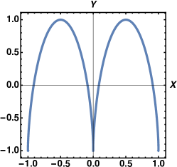
(b)   Singular Normalized Profile

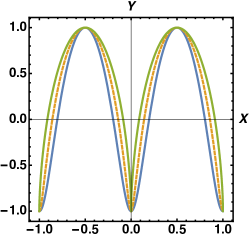
(c)   Regular and Nonregular Profiles

Figure 7: The selected threshold $J_{d}$ as a function of $2\pi d$, where $d$ is the ratio between of thickness to pattern wavelength. For a thin film, the threshold increases dramatically as $J_{d}\sim 4.93347/(2\pi\Lambda d)$. When the thickness is of order or greater than $\Lambda/\pi$, $J_{d}$ reaches the asymptotic limit $J_{d}\sim J_{\infty}=J_{b}$, so $3.3829$ represented by a solid blue line in (a). In the inset, the critical amplitude ${\cal A}$ defined in eq.(148) (in units of the wavelength for observing a crease with a single harmonic mode). A plateau of order $0.3$, is reached very quickly. In b) a normalized pattern is plotted for a value of ${\cal A}$ at the critical value $0.3$ where $d=t_{3}/\pi$ and $J_{c}$ the threshold value. The amplitude $x$ is divided by ${\cal A}$ for normalization. A cusp can be observed for $Y=0$, which repeats periodically for $Y=n\pi$. In c) superposition of the profiles for increasing amplitudes for ${\cal A}=0.1$ in blue, ${\cal A}=0.2$ and ${\cal A}=0.3$.

XIII Finite-size effects or the buckling of layers

One may wonder whether the degeneracy of the solutions presented above is not due either to the simplicity of the neo-Hookean model or to the fact that the initial geometry is too simple. It is obvious that a length scale is missing in our formulation, since we arbitrarily set the wavelength to unity. Consider the case of a gel layer whose height is given by the parameter $d$. In order to keep as much as possible the same definitions and equations given in the previous section, we continue to use the wavelength as the unit of length. This situation was also considered by Biot in 1963, but with different boundary conditions [23] and with a different point of view: the limit of small height $d$ compared to the wavelength where the analogy with Euler’s buckling becomes more explicit [23]. Sinusoidal modes have been found and the dispersion relation given the wavelength as a function of $d$ has been given numerically. In this section, our aim is to revisit his results with different boundary conditions at the substrate and considering $d>1$. For a single layer, there is no need to change the main equations, just remember that boundary conditions have to be applied on both horizontal sides $X=0$ and now $X=d$ and during the growth, the layer can be free or glued at the bottom. In the first case, and unlike the second case, symmetry allows us to choose half of the sample with boundary conditions for $X=d/2$, which is now the bottom. In any case, we will have strain conditions at the bottom and free stress conditions at the top: $X=0$. These two cases are physically similar and will only differ in numerical values. The two sets of boundary conditions to be applied either at the top or at the bottom are different in nature, and due to the finite extension of the layer, divergent solutions at infinity are now relevant. They were not allowed and eliminated in the previous section. The non-symmetric case adapts more easily to bilayers and is therefore of more interest. This is especially true when the second layer is stiffer than the upper layer (see [8]) although the case of a soft substrate is more considered in the literature [175, 176, 177, 178]. Under growth, the description of the new positions $(x,y)$ can follow the same perturbation scheme as before, but must now include $2$ holomorphic functions: $\Phi_{e}(Z)$, (an even function of $Z$) and $\Phi_{o}(Z)$ (an odd function of $Z$). Then, by defining $\tilde{Z}=Z-d=X+IY-d$ and $\tilde{Z}_{1}=Z_{1}-Jd=J(X-d)+IY$, the Euler-Lagrange equation associated with the incompressibility condition gives the following results for the deformations:

$$\begin{cases}x=JX-(J-1)d+J\epsilon\Re\,[F_{1}(\tilde{Z})+F_{2}(\tilde{Z}_{1})]\,,\\ y=Y-\epsilon\Im\,[F_{1}(\tilde{Z})+JF_{2}(\tilde{Z}_{1})]\,.\\ \end{cases}$$ (141)

where

$$\begin{cases}F_{1}=\Phi_{e}(\tilde{Z})+a_{1}\Phi_{o}(\tilde{Z})\,,\\ F_{2}=b_{1}\Phi_{e}(\tilde{Z}_{1})+b_{2}\Phi_{o}(\tilde{Z}_{1})\,.\end{cases}$$ (142)

With this definition, the incompressibility condition valid everywhere in the sample:

$$\frac{\partial(x-JX)}{\partial X}+J\frac{\partial(y-Y)}{\partial Y}\quad\forall\quad X\quad{\mbox{and}}\quad Y\,,$$ (143)

is automatically checked at first order in $\epsilon$. The boundary conditions of anchoring to the solid substrate impose: $x=d$ and $y=Y$ for $X=d$. Since $\Re\,\,[\Phi_{o}(IY)]$ and $\Im\,[\Phi_{e}(IY)]$ vanish independently of the $Y$ values, the anchorage then imposes $b_{1}=-1$ and $b_{2}=-a_{1}/J$. It remains to apply the free stress conditions involving $S_{11}$ and $S_{21}$ on the upper boundary (X=0) which must be verified for arbitrary $Y$ values. Let us limit ourselves to the harmonic modes.

XIII.1 Selection of a unique harmonic mode

Selecting $\Phi_{e}(Z)=\cosh(2\pi Z)$ and $\Phi_{o}(Z)=\sinh(2\pi Z)$, to represent the current $(x,y)$ coordinates, the first order incremental correction in $\epsilon$ becomes: $\delta x=J\cos(2\pi Y)f_{1}(\tilde{X},X_{1})$ and $\delta y=\sin(2\pi Y)f_{2}(\tilde{X},\tilde{X}_{1})$, where $\tilde{X}=2\pi(X-d)$ and $\tilde{X}_{1}=2\pi J(X-d)$ and

$$\begin{cases}f_{1}&=\cosh\tilde{X}-\cosh\tilde{X}_{1}+a_{1}(\sinh\tilde{X}-\frac{\sinh\tilde{X}_{1}}{J})\,,\\ f_{2}&=a_{1}(\cosh\tilde{X}_{1}-\cosh\tilde{X})+J\sinh\tilde{X}_{1}-\sinh\tilde{X}\,.\end{cases}$$ (144)

Now, considering the cancellation of the normal $S_{11}$ and of the shear stress $S_{21}$ at the top of the strip, we derive the value of the coefficient $a_{1}$ in a first step:

$$a_{1}=\frac{J(2J\sinh(\tilde{d})-(1+J^{2})\sinh(J\tilde{d})}{2J^{2}\cosh(\tilde{d})-(1+J^{2})\cosh(J\tilde{d})}\,,$$ (145)

where $\tilde{d}=2\pi d$. The dispersion relation ${\cal D}$ gives the new threshold $J_{d}$ as a function of the ratio of wavenumber to thickness, so $2\pi d$ is the solution of a transcendental equation:

$${\cal D} =-4J_{d}^{2}(1+J_{d}^{2})+(1+2J_{d}^{2}+5J_{d}^{4})\cosh(\tilde{d})\cosh(J_{d}\tilde{d})\,,$$ (146)

$$-J_{d}(1+6J_{d}^{2}+J_{d}^{4})\sinh(\tilde{d})\sinh(J_{d}\tilde{d})=0\,,$$

XIII.2 Nonlinearity and creasing above threshold for growing layer

Why focus on a single harmonic mode? Each harmonic mode will correspond to $\cosh(2\pi mZ)$ and $\sinh(2\pi mZ)$ and will have a different threshold given by $J_{md}$ as opposed to the unique threshold independent of $m$ for an infinite thickness, see section (IX.3). Thus, we cannot simply combine different modes and evaluate the nonlinearities. In fact, nonlinear profiles do not result from a single mode and traditional techniques become more difficult. Other asymptotic techniques consist of the coupling mode approach of classical bifurcation theory such as the Landau formalism of the amplitude equations [32, 33, 118, 34] but it remains complex or even impossible to use them with partial differential equations with boundary conditions. One method, different from the present one, concerns the use of a nonlinear stream function introduced in [19], which exactly treats the incompressibility and reports the nonlinearities on the elastic energy [7, 52, 8]. This method, valid only in $2D$ geometry or when the elastic deformations are reduced to a two-dimensional space, has allowed to demonstrate a third order of expansion: [19] :

$$\begin{cases}x=JX-(J-1)d+\epsilon J\cos(2\pi y)f_{1}\,,\\ Y=y-\epsilon\sin(2\pi y)f_{2}\,.\end{cases}$$ (147)

The parameter $\epsilon$ being predicted at the third order. Of course, this prediction depends on the size of the layer $d$. This formulation assumes that all inversion formulas can be achieved, which is obviously not the case when creases occur at the interface. They appear when $\partial Y/\partial y$ vanishes for $X=0$ according to the theorem of the implicit function, ([32]), which gives the critical value ${\cal A}$, which is equal to $\epsilon Jf_{1}$ of the deformation at the cusp position (see inset in Fig.(7), panel (a)) and eq.(147). It can be noticed that the required amplitude saturates to a finite value around 0.3 for values $d$ of the sample width of the order of the wavelength or more, and that very thin samples, very easily exhibit cusps as they grow, although their threshold $J_{d}$ is obtained for a higher value. In Fig.(7), panel (b) we plot the profile of the cusp function over one period. It is divided by ${\cal A}$ for normalization so that the amplitude varies between $-1$ and $1$. To evaluate whether the amplitude ${\cal A}$ can be obtained in practice requires an analytical treatment of the nonlinearities (which is not reported here, see Ref.([8]). It approximates the amplitude of the wavy regular pattern above the bifurcation threshold $J_{d}$ as

$$x\sim-(J-1)d\pm 0.537\sqrt{J-J_{d}}\cos(2\pi Y)$$ (148)

where the numerical number $0.537$ is analytically predicted and the zero order in eq.(148) indicates the increase in height due to growth, which appears negative due to our choice of coordinate system. The nonlinear treatment assumes a regular wave pattern and does not assume a priori singularities as cusps. This estimation must be compared with the amplitude ${\cal A}$ and results in a growth parameter inducing a possible crease given by ${\cal A}\sim 0.3=0.537\sqrt{J-J_{d}}$, which implies a distance from the threshold approximately equal to $0.3$, or $10\%$ of the Biot threshold. Thus, for a thickness of the order of the pattern wavelength: $d/\Lambda\sim 1$, creases appear rather quickly at the interface once the threshold value is exceeded. Although nonlinearities can be responsible for creases, they always appear above the Biot threshold and not below.

XIII.3 Conclusion

We have shown that the sinusoidal Biot profile is not the only solution that occurs in a growing hyperelastic sample. Restricting to the simplest configuration of a semi-infinite two-dimensional neo-Hookean sample, growing with an isotropic constant growth rate $J$, we show that other candidates are possible solutions that appear exactly at the same threshold. Among them, quasi-singular solutions with a periodic array of cusps can be found, at the Biot threshold. Nonlinearities can be evaluated by classical nonlinear treatments, supercritical bifurcations are rather common, but also subcritical bifurcations can appear slightly below the Biot threshold when several harmonics are coupled. This explains the diversity of experimental observations independent of the elasticity model, since this diversity occurs at the level of the simplest growth formalism. Independent of these patterns, which are always related to the Biot threshold, it has been suggested that patterns can occur well below the Biot threshold if local singularities also occur within the material. We consider this conjecture and show that it can be the source of new families of solutions. In this case, tiny linear singularities occur through pairs near (but not at ) the interface where the compressive elastic field is concentrated. The high level of stress generated requires a slight local modification of the elastic model. Relevant parameters such as the linear extension of the singularities and their positions are recovered by path-independent integrals. In addition, this study proposes a threshold value for the volumetric growth below the Biot threshold determined by the nonlinearities above the neo-Hookean approach.

XIV Acknowledgements

I would like to thank Linda Cummings, Darren Crowdy and Saleh Tanveer for insightful discussions during the programme ”Complex analysis: techniques, applications and computations” (Fall 2019, July 2023) of the Isaac Newton Institute of Mathematical Sciences, Cambridge, for its support and hospitality. I acknowledge the support of the ANR (Agence Nationale de la Recherche) under the contract MecaTiss (ANR-17-CE30-0007) and the contract EpiMorph (ANR-2018-CE13-0008).

XV Appendix

XV.1 Nonlinear elasticity at first order: stress and energy expansion

This appendix is written with the elastic fields given by a complex function. It is written in the initial frame of coordinates and the stress corresponds to the Piola stress tensor[93].

$$x = JX+\epsilon J\Re\,\,[\Phi(Z)+\tau_{1}\Phi(Z_{1})]\,,{}$$

$$y = Y-\epsilon\Im\,[\Phi(Z)+\tau_{1}J\Phi(Z_{1})]\,.$$ (S1)

In this work, we restrict to $\Phi=\bar{\Phi}$ or $\Phi$ function having a real expansion in $Z$. The Jacobian in $2D$ is given by $I_{3}=x_{X}\cdot y_{Y}-x_{Y}\cdot y_{X}-J$. At linear order it reads:

$$x_{X} = J+\epsilon J\Re\,\,[\Phi_{Z}+J\tau_{1}\Phi_{Z_{1}}]\,,{}$$

$$y_{Y} = Y-\epsilon\Re\,\,[\Phi_{Z}+J\tau_{1}\Phi_{Z_{1}}]\,,{}$$

$$x_{Y} = -\epsilon J\Im\,[\Phi_{Z}+\tau_{1}\Phi_{Z_{1}}]\,,{}$$

$$y_{X} = -I\epsilon\Im\,[\Phi_{Z}+J^{2}\tau_{1}\Phi_{Z_{1}}]\,.$$ (S2)

With this choice for the deformation field, we can verify that at linear order in $\epsilon$, $I_{3}=0$ as required.

The Euler-Lagrange equation for the Neo-Hookean model are given by:

$$\Delta x=x_{XX}+x_{YY}=Q_{X};\,\,\Delta y=y_{XX}+y_{YY}=JQ_{Y}\,.$$ (S3)

Obviously, only the term depending on $Z_{1}$ and $\bar{Z}_{1}$ are concerned by these equations which implies that the Lagrange parameter $Q$ is only a function of $Z_{1}$ and $\bar{Z}_{1}$. Both equations of eq.(S3) determines $Q$ as:

$$Q=J+\frac{1}{2}\epsilon\tau_{0}\tau_{1}\left\{\Phi_{Z_{1}}+\tilde{\Phi}_{Z_{1}}\right\}$$ (S4)

It remains to check that the boundary verifies the cancellation of the shear $S_{21}$ and normal stress $S_{11}$ for the free surface $X=0$. Using eq. (XV.1), we first obtain the components of the Piola stress tensor. For the diagonal elements:
$S_{11}=x_{X}-Qy_{Y}$ and for $S_{22}=y_{Y}-Qx_{X}$:

$$\begin{cases}S_{11}&=\epsilon\Re\,[2J\Phi_{Z}+(1+J^{2})\tau_{1}\Phi_{Z_{1}}]\,,\\ S_{22}&=-\tau_{0}-\epsilon\Re\,[(1+J^{2})\Phi_{Z}+2J^{3}\tau_{1}\Phi_{Z_{1}}]\,.\end{cases}$$ (S5)

For the off-diagonal elements, we have:

$S_{21}=y_{X}+Qx_{Y}$ and $S_{12}=x_{Y}+Qy_{X}$ which reads:

$$\begin{cases}S_{21}&=-\epsilon(1+J^{2})\Im\,[\Phi_{Z}+2J^{2}\tau_{1}\Phi_{Z_{1}}],\\ S_{12}&=-\epsilon\Im\,[2J\Phi_{Z}+(1+J^{2})\tau_{1}\Phi_{Z_{1}}].\end{cases}$$ (S6)

Note that, for $X=0$ so for $Z=IY$, the normal stresses on the top stress become:

$$S_{11}=\frac{1}{2}(2J+(1+J^{2})\tau_{1})(\Phi_{Z}+\bar{\Phi}_{\bar{Z}})\,,$$ (S7)

$$S_{21}=\frac{I}{2}(1+J^{2}+2J^{2}\tau_{1})(\Phi_{Z}-\bar{\Phi}_{\bar{Z}})\,.$$ (S8)

The boundary conditions impose $S_{11}=S_{21}=0$ but If $\Phi(Z)$ is an even function of $Z$, the derivative $\Phi^{\prime}(Z)$ is odd, so $S_{11}$ vanishes automatically, and we only need to choose $\tau_{1}=-(1+J^{2})/(2J^{2})$ to cancel $S_{21}$. If $\Phi(Z)$ is an odd function of $Z$, then $S_{21}$ cancels automatically and $S_{11}=0$ imposes $\tau_{2}=-2J/(1+J^{2})$. Our choice in this manuscript corresponds to the first case. The Biot solution $\Phi(Z)=e^{-2\pi Z}$ has no parity so both normal stress components must vanish at the top of the strip $X=0$, which explains the existence of the threshold $J=J_{B}$. Regardless of the choice of $\tau_{1}$ or $\tau_{2}$, the threshold value $J_{B}$ is identical.

XV.2 Expansion of the elastic and capillary energy density

Expansion of the the elastic energy density $E$ given by eq.(45) at third order of the parameter $\epsilon$: $E=E_{0}+\epsilon E_{1}+\epsilon^{2}E_{2}+\epsilon^{3}E_{3}$, reads:

$$\begin{cases}E_{0}=\frac{1}{2}(J-1)^{2}\,,\\ \\ E_{1}=\tau_{0}\Re\,[\Phi_{Z}+J\tau_{1}\Phi_{Z_{1}}],\\ \\ E_{2}=\frac{1}{2}(3J^{2}+1)(|\Phi_{Z}|^{2}+J^{2}\tau_{1}^{2}|\Phi_{Z_{1}}|^{2})\\ +\frac{J\tau_{1}}{2}\Re\,[(J+1)^{3}\Phi_{Z}\Phi_{\bar{Z}_{1}}-(J-1)^{3}\Phi_{Z}\Phi_{{Z_{1}}}])\,,\\ \\ E_{3}/(J\tau_{0}\tau_{1})=\Re\,[\Phi_{Z_{1}}]\times(|\Phi_{Z}|^{2}+J^{2}\tau_{1}^{2}|\Phi_{Z_{1}}|^{2}\\ +\frac{\tau_{1}}{2}\Re\,[(J+1)^{2}\Phi_{Z}\Phi_{\bar{Z}_{1}}-(J-1)^{2}\Phi_{Z}\Phi_{Z_{1}}])\,.\end{cases}$$ (S9)

Note that if $J=1$ (no growth) all the coefficients $E_{i}$ vanish whatever the function $\Phi(Z)$.

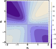
(a)    $\bm{e_{3}}$ coefficient

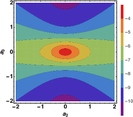
(b)     $\bm{g_{2}}$ coeffient

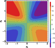
(c)    $\bm{g_{3}}$ coefficient

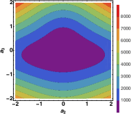
(d)     $\bm{g_{4}}$ coefficient

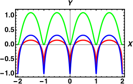
(e)   Profile for an outer Logarithmic singularity

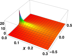
(f)  Real Part

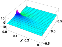
(g)  Imaginary part

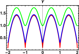
(h)  Profile for an outer square root singularity

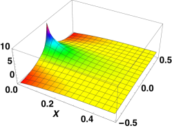
(i)  Real Part

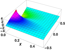
(j)  Imaginary part

Figure 8: In (a) and (b) density plots of the coefficients $e_{3}$ and $g_{2}$ entering the expansion of the free energy eq.(S16) as a function of $a_{2}$ and $a_{3}$. The numerical values can be estimated from the legend to the right of each panel. In (c) and (d) Density plots of the coefficients $g_{3}$ and $g_{4}$ entering the expansion of the free energy eq.(S16) as a function of $a_{2}$ and $a_{3}$.
In (e) the interface profile for a logarithmic singularity according to eq.(63) with the parameter $a=0.01$ for the red curve, $a=0.1$ for the blue curve, $a=1.$ for the green curve. For $a=1$ the definition is changed and the plot only concerns $\Re\,[\Phi(\zeta_{a})]$, while for $a=0.01$ or $a=0.1$, it is given by eq.(63). In the second row, in (h), the interface profile for a square root singularity according to eq.(63) with the parameter $a=0.01$ for the red curve, $a=0.1$ for the blue curve, $a=1.$ for the green curve. In (f,i), the real part of the $\Phi(Z)$ derivative contributes to the stress, see $S_{11}$, eq.(S5). In (i,j) the imaginary part is shown, it goes into the formula for $S_{21}$. One wavelength ${\mathcal{P}}$ is shown and the rainbow colors indicate the sharp variations near the origin $\mathcal{O}$. Note also that the scale for $X$ varies from $0$ to $0.3$ for (f,g), and from $0$ to $0.5$, for (i,j). Although quite singular near $\mathcal{O}$, the stress remains finite and goes to zero very quickly.

The capillary energy density evaluated at $X=0$ so for $Z=IY$ can be expanded up to forth order:

$${\cal E}_{c}=\gamma_{0}\epsilon(E_{1c}+\epsilon E_{2c}+\epsilon^{2}E_{3c}+\epsilon^{3}E_{4c})\,,$$ (S10)

where $\gamma_{0}$ is the ratio between the capillary energy and the shear modulus multiplied by the wavelength and where:

$$\begin{cases}E_{1c}=\frac{(J-1)^{2}}{2J}\Re\,[\Phi_{Z}]\,,\\ \\ E_{2c}=\frac{\tau_{0}^{2}}{8J^{2}}(\Im\,[\Phi_{Z}])^{2}\,,\\ \\ E_{3c}=-\frac{\tau_{0}^{2}(J-1)^{2}}{16J^{3}}\Im\,[\Phi_{Z}]^{2}\Re\,[\Phi_{Z}]\,,\\ \\ E_{4c}=\frac{\tau_{0}^{2}(J-1)^{2}}{128J^{4}}\Im\,[\Phi_{Z}]^{2}\times\\ \{(5-6J+5J^{2})\Re\,[\Phi_{Z}]^{2}-(J+1)^{2}|\Phi_{Z}|^{2}\}\,.\end{cases}$$ (S11)

XV.3 Evaluation of the total energy for a single mode, double and triple mode

We consider first a single mode: $\zeta=e^{-2\pi Z}$. in this case, only $E_{2c}$ and $E_{4c}$ and $E_{6c}$ contribute to the capillary energy $E_{cs}$. After integrating on the top interface and defining the following quantities:

$$\begin{cases}\alpha_{c}=\left(\frac{(J-1)\pi}{2J}\right)^{2};E_{s0}=\gamma_{0}\alpha_{c}\epsilon^{2}(1+J)^{2},\\ \\ {\cal Q}_{1c}=\frac{1}{4}(J^{2}-14J+1),\\ \\ Q_{2c}=\frac{1}{4}(1-12J+102J^{2}-12J^{3}+J^{4}).\end{cases}$$ (S12)

it reads:

$${\cal E}_{cs}=E_{s0}\left(1+\epsilon^{2}\alpha_{c}{\cal Q}_{1c}+\epsilon^{4}\alpha_{c}^{2}{\cal Q}_{2c}\right)$$ (S13)

If the base state includes other harmonics such as $\zeta^{2}$ and $\zeta^{3}$ with decreasing amplitudes as in section IX.5, $\phi[Z]=\zeta+\epsilon B_{2}\zeta^{2}-\epsilon^{2}B_{3}\zeta^{3}$, the capillary energy includes ${\cal E}_{cs}$ but also additive terms in $\epsilon^{4}$ and $\epsilon^{6}$:

$${\cal E}_{c}={\cal E}_{cs}+E_{s0}\epsilon^{2}\left(e_{1c}++\epsilon^{2}e_{2c}\right).$$ (S14)

$$\begin{cases}e_{1c}=B_{2}(4B_{2}+\pi(J-1)^{2}/J),\\ e_{2c}=9B_{3}^{2}-\frac{3\alpha_{c}}{\pi}B_{3}(8JB_{2}+\pi(1+J)^{2})\\ +4\alpha_{c}Q_{1c}e_{1c}.\end{cases}$$ (S15)

We now consider the 3 mode coupling with $\Phi(Z)=\zeta+a_{2}\zeta^{2}+a_{3}\zeta^{3}$ of the section IX.4.2. The goal is to evaluate the weight of each term in the expansion of the elastic energy, eq.(85), and to compare it with the capillary energy. Writing the total energy: the elastic plus the capillary energy, we obtain for ${\cal E}_{t}=-E_{f}\epsilon^{2}{\cal\tilde{E}}_{t}$ (see eq.(85)) where:

$$\begin{cases}E_{f}=\pi{\cal Q}_{2}(1+2a_{2}^{2}+3a_{3}^{2})\,,\\ {\cal\tilde{E}}_{t}=\delta J+2\gamma_{0}g_{2}+(e_{3}+2\gamma_{0}g_{3})\epsilon+2\gamma_{0}g_{4}\epsilon^{2}.\end{cases}$$ (S16)

where ${\cal Q}_{2}$ has been given in eq.(74), $e_{3}$ in eq.(88) and $e_{4}=0$:

$$e_{3}=\pi^{2}a_{2}{\cal Q}_{3}(1+a_{3}{\cal Q}_{33})/E_{f};\,g_{i}=-E_{ic}/E_{f}\\$$ (S17)

We first define:

$$f_{g}=-\frac{(-1+J)^{2}(1+J)}{(1+2a2^{2}+3a3^{2})(3J^{2}-6J-1)}$$ (S18)

$$\begin{cases}g_{2}=(1+4a_{2}^{2}+9a_{3}^{2})\frac{J\pi f_{g}}{(J-1)^{2}},\\ g_{3}=a_{2}(1+6a_{3})\pi^{2}f_{g},\\ g_{4}=\frac{\pi^{3}f_{g}}{4J}\{3a_{3}(1+J)^{2}+Q_{1c}\times(1+36a_{3}^{2}\\ +81a_{3}^{4}+16a_{2}^{2}(1+a_{2}^{2}+3a_{3}+9a_{3}^{2})\}\end{cases}$$ (S19)

$E_{f}$ is positive and all polynomials must be evaluated for $J=J_{B}$. The order of magnitude of each coefficient as $e_{3},g_{2},g_{3},g_{4}$ is function of the two parameters $a_{2}$ and $a_{3}$, once $J=J_{B}$ is imposed and is represented by density plots (see Fig.(8)). More specifically, Fig.(8(a) gives the order of magnitude of $e_{3}$ while panel (b) gives the $g_{2}$ coefficient as function of the same quantities. $g_{2}$ is negative and so is responsible for shifting the threshold towards higher values, a similar result was found in [19]. Fig.(8c) and Fig.(8d) are dedicated respectively to $g_{3}$ and $g_{4}$ respectively. Note that all $g_{i}$ must be multiplied by the capillary number $\gamma_{0}$ and only $g_{4}$ appears alone in the asymptotics eq.(S16).

XV.4 Profiles and Cartography of the stress

The profiles and the stress of both a logarithmic singularity and of a square root singularity, localized outside the elastic sample, are displayed in Fig. (8). Panels (e,f,g) are devoted to $\Phi(Z)=-Log1+a-e^{-2\pi Z}/Log(a)$ for $a=0.01,0.1$ and to $\Phi(Z)=Log(2-e^{-2I\pi Y})$ for $a=1$. This corresponds to singularities in the physical plane located to a distance $d_{a}=-0.00158,-0.01516,-0.110318$, outside the elastic sample. The panels (h,i,j) concern the square root singularity:$\sqrt{e^{-2\pi Z}-1-a}$. An indication of the normal stress $S_{11}$, which includes the real part of $\Phi_{Z}$, and the shear stress $S_{21}$, which includes the imaginary part are also shown in panels (f,i) and (g,j) of Fig.(8). The stress contributes significantly at the boundary, but decreases very rapidly. $S_{11}$ and $S_{21}$ are given by eq.(S5).

XV.5 Weakly nonlinear analysis for quasi-singular profiles

These profiles have been discussed in section (VIII.2. A full exhaustive study cannot be achieved and it iis not certain that the method of weakly nonlinear analysis will converge for these choices of quasi-singularity. The evaluation of the integrals is not easy in $X$ and $Y$ geometry and and we choose a particular mode: $\phi(Z)=-(Log(1+a-e^{-2\pi Z})-Log(1+a))/Log(a)$. Obviously, an expansion in sinusoidal modes: $\zeta^{p}$ have little chance to converge quickly so we have to modify our strategy. The algebra is more complex even with formal mathematical software and we cannot find in handbooks of integrals the result for the previously defined integrals that go into the energy expansion. Thus, the results cannot be obtained completely analytically without approximations. It is also not possible, except for $L_{3}$, to integrate in the complex plane of $\zeta$ or the physical plane $\Omega$ due to the juxtaposition of $Z$ and $Z_{1}$. Let us give an estimate. A first integration on $Y$ induces the evaluation of two kinds of integrals, ${\cal L}_{m,n}$ :

$${\cal L}_{m,n}=\int_{0}^{\infty}\frac{e^{-2\pi(m+n)u}du}{\left(\alpha^{2}-e^{-2\pi mu}\right)\left(\alpha^{2}-e^{-2\pi nu}\right)}\,,$$ (S20)

where $m$ and $n$ are positive integers,$\alpha=a+1$. Using Watson’s lemma [179] and the fact that the denominator is singular near $X=0$ for vanishing $a$ values, once the parameter $l_{m}$ is introduced with $l_{m}=a(2+a)/(2m\pi)$, we approximate the denominator by linear expansion giving

$${\cal L}_{m,n}\sim\int_{0}^{\infty}\frac{du}{p_{a}}e^{-2\pi(m+n)u}\left(\frac{1}{l_{m}+u}-\frac{1}{l_{n}+u}\right)\,,\\$$ (S21)

with $p_{a}=2\pi a(2+a)(m-n)$. The two last integrals can be computed explicitly with the function exponential integrals $(E_{i})$ and the limit $l_{m}->0$ finally gives the following result:

$${\cal L}_{m,n}\sim\frac{1}{4\pi a}l_{m,n}+O(a)\,\,\mbox{with}\,\,l_{m,n}=\frac{Log(m/n)}{m-n}\,.$$ (S22)

For $m=n$, $l_{n,n}=1/n$. Then, taking into account only the contribution in $a^{-1}$ and defining $m_{a}=-2\pi^{2}/(aLog(a)^{3})$, we get:

$$\begin{cases}L_{1}&\sim m_{a}l_{2,1+J}=\frac{m_{a}}{1-J}Log\frac{2}{1+J}\,,\\ L_{2}&=m_{a}l_{2J,2J}=\frac{m_{a}}{2J}\,,\\ L_{4}&\sim\frac{m_{a}}{2}l_{2J,1+J}=\frac{m_{a}}{2(J-1)}Log\frac{2J}{1+J}\,,\\ L_{3}&\sim\frac{m_{a}}{2}(l_{1+J,1+J}+l_{2J,1+J})\\ &\sim\frac{m_{a}}{2}\left(\frac{1}{1+J}+\frac{Log(2J/(1+J))}{J-1}\right)\,.\\ \end{cases}$$ (S23)

A comparison between numerical values of integrals (see eq.(S20) and the estimate given by eq.(S22) is correct for $a\sim 0.01$, but smaller values are necessary for eq.(S23). This treatment can always be done numerically, the advantage here is to find the scaling of ${\cal E}_{3}$. For the logarithmic choice, we finally derive:

$$\begin{cases}\Pi_{1}\sim 4J^{2}(J+1)^{2}Log\left(\frac{2}{J+1}\right)\\ +\left(J^{2}+1\right)\left(4J^{2}Log(J)+(J-1)^{2}\right)\,,\end{cases}$$ (S24)

and the third order correction gives:

$${\cal E}_{3}=-\frac{(J+1)}{8J^{2}}\Pi_{1}\tau_{1}m_{a}\simeq-\frac{38.38}{aLog(a)^{3}}\,.$$ (S25)

XV.6 Path-independent integrals

It may seem pointless to demonstrate that conservation laws remain valid in incremental models of finite elasticity after the pioneering work of Knowles and Sternberg [171], but there are some slight differences with our approach. Fist, we are concerned with growth so our initial state is an anisotropic (axially pre-stretched) state. Second, our demonstration is achieved at the second order in $\epsilon$ and not at first order. For this reason, if we can predict the result for the $J$ integral, it is less obvious for the $M$ integral, which is not believed to be valid in nonlinear elasticity. The strategy to prove the existence of path-independent integrals is simple: it consists in relating a scalar or a vector to a vector or a tensor which is divergence free. In $2$ dimensions, we shall demonstrate that it is the case for $\cal J$ and $\cal M$. First let us begin by ${\cal J}$

$${\cal J}_{i}=\iint dS\left\{\frac{\partial(E\delta_{ik})}{\partial X_{k}}-\frac{\partial(S_{jk}F_{ji})}{\partial X_{k}}\right\}\,.$$ (S26)

where we use the Einstein convention for repeated indices and $dS=dXdY$ and the brackets represent ${\cal T}_{i}$ The index $i$ reminds us that the $J$ integral is indeed a vector but here only the component $\vec{\bf e}_{X}$ is important. $\bf F$ is the gradient of the deformation tensor, whose components are: $F_{ij}=\partial x_{i}/\partial X_{j}$. It can be replaced by $\bf U$ so that $U_{ij}=F_{ij}$ if $i\neq j$ and $U_{11}=F_{11}-J$ and $U_{22}=F_{22}-1$. We want to show that ${\cal T}_{i}$ is a divergence. In $2$ dimensions, we have :

$${\cal T}_{1}=\frac{\partial E}{\partial X}-\frac{\partial(S_{11}U_{11}+S_{21}U_{21})}{\partial X}-\frac{\partial(S_{12}U_{11}+S_{22}U_{21})}{\partial Y}\,.$$ (S27)

where $E$ has been given in eq.(45), $\bf S$ is the Piola stress tensor already defined in eq.(58). At equilibrium, the divergence of the Piola stress tensor cancels:

$$\frac{\partial S_{11}}{\partial X}+\frac{\partial S_{12}}{\partial Y}=0\quad\frac{\partial S_{21}}{\partial X}+\frac{\partial S_{22}}{\partial Y}=0\,.$$ (S28)

$$\begin{cases}{\cal T}_{1}&=\frac{\partial E}{\partial X}-\left(S_{11}\frac{\partial^{2}x}{\partial X^{2}}+S_{21}\frac{\partial^{2}y}{\partial X^{2}}\right)\\ \\ &-\left(S_{12}\frac{\partial^{2}x}{\partial X\partial Y}+S_{22}\frac{\partial^{2}y}{\partial X\partial Y}\right).\end{cases}$$ (S29)

We recall the Piola stress components, given in section VII.2, Eqs.(50,53), that we evaluate at linear order in $\epsilon$:

$$\begin{cases}S_{11}=\frac{\partial x}{\partial X}-Q\frac{\partial y}{\partial Y}\quad S_{12}=\frac{\partial x}{\partial Y}+Q\frac{\partial y}{\partial X}\,,\\ \\ S_{21}=\frac{\partial y}{\partial X}+Q\frac{\partial x}{\partial Y}\quad S_{22}=\frac{\partial y}{\partial Y}-Q\frac{\partial x}{\partial X}\,.\end{cases}$$ (S30)

From eq. (S29) it is easy to show that all terms of the neo-Hookean part are eliminated by the stress contribution of the same equation and that terms proportional to $Q$ also cancel each other, a relation which is always true even without expansion in $\epsilon$. So ${\cal T}_{1}$ vanishes and the same result is obtained for ${\cal T}_{2}$. In our case, ${\cal J}_{1}$ and an ${\cal J}_{2}$ vanishes rigorously on a closed contour, and so also up to second order. Although ${\cal J}_{2}$ vanishes identically in our geometry because of the chosen contour, we write its generic form, which will be useful to establish the $\cal M$ integral:

$$\begin{cases}{\cal T}_{2}=\frac{\partial E}{\partial Y}\\ -\frac{\partial(S_{11}U_{12}+S_{21}U_{22})}{\partial X}-\frac{\partial(S_{12}U_{12}+S_{22}U_{22})}{\partial Y}\,.\end{cases}$$ (S31)

Let us consider now ${\cal M}=\iint dSN$

$$N=\frac{\partial\delta EX_{i}}{\partial X_{i}}-\frac{\partial\left(S_{jk}U_{ji}X_{i}\right)}{\partial X_{k}}-\tau_{0}/J\frac{\partial U_{X}}{\partial X}\,.$$ (S32)

where $\delta E=E-(J-1)^{2}/2$, $U_{i}$ is the displacement: $U_{1}=x-JX$ and $U_{2}=y-Y$. The last term can be replaced by $-(1+J)Div(U)=-(1+J)(\partial_{X}U_{X}+\partial_{Y}U_{Y}$. This result, which is easy to demonstrate with mathematica software, turns out to be less obvious to show analytically and differs from the result obtained by Knowles and Sternberg for incremental elasticity. The reason is due to growth since $J^{2}-1$ different from from zero, in our case. Nevertheless, our definition of $M$ satisfies the criterion for defining a path independent integral similar to the classical $M$ integral of linear elasticity up to order $\epsilon^{2}$. After some algebra with this definition, which is slightly different from the one given by [171], we can construct a path-independent integral, valid up to second order for a pre-stretched sample. Compared to eq.(3.36) of [171]’s equation, the only difference comes from the last term of the previous equation. Transforming ${\cal M}$ into a closed contour integral: ${\cal M}=\oint ds{\it m}=0$

$$\begin{cases}{\it m}=\left(E-\frac{(J-1)^{2}}{2}\right)\vec{\bf X}.\vec{\bf N}-S_{jk}U_{ji}X_{i}.N_{k}\\ -(J+1)\left\{(x-JX)\cdot N_{X}+(y-Y)\cdot N_{Y}\right\}\,.\end{cases}$$ (S33)

This result is true up to $O(\epsilon^{3})$. Then the horizontal boundary at the top contributes to the order of $\epsilon$. We have already discussed the case of two boundaries in the main text section (XII.2). For completeness we will also consider the patches here, at least to confirm our approach. Considering now the $2$ patches where the function $F$ or $\Phi$ has singularities in $X=X_{0}$ and $X=X_{0}/J$, we can then consider $3$ contributions. We start with a separation into three contributions for ${\cal M}_{{\cal J}_{S}}$ into: ${\cal M}^{(1)}+{\cal M}^{(2)}+{\cal M}^{(3)}$ which will be done for the two patches one after the other. Around the patch located at $X=X_{0}$, the contour being a circle with radius $R$ greater than $l_{0}$ but less than $X_{0}$, definined by

$$\begin{cases}m_{1}&=E-\frac{(J-1)^{2}}{2}-S_{11}U_{11}-S_{21}U_{21},\\ m_{3}&=E-\frac{(J-1)^{2}}{2}-S_{12}U_{12}-S_{22}U_{22},\\ m_{2}&=S_{12}U_{11}+S_{22}U_{22},\\ m_{4}&=S_{11}U_{12}+S_{21}U_{22}.\end{cases}$$ (S34)

Note that each $m_{i}$ is of order $\epsilon^{2}$

$${\cal M}_{{\cal J}_{S}}=R\int_{-\pi}^{\pi}dT(X_{0}+R\cos{T})\left\{\cos{T}m_{1}-m_{2}\sin{T}\right\}\,.$$ (S35)

This relation can eventually be simplified to give:

$${\cal M}^{(1)}_{{\cal J}_{S}}=X_{0}{\cal J_{S}}+R^{2}\int_{-\pi}^{\pi}dT\cos{T}(\cos{T}m_{1}-\sin{T}m_{2})\,.$$ (S36)

Defining in the same way:

$${\cal M}^{(2)}_{{\cal J}_{S}}=R^{2}\int_{-\pi}^{\pi}dT\sin{T}\left\{\sin{T}m_{3}-\cos{T}m_{4}\right\},$$ (S37)

and finally:

$${\cal M}^{(3)}_{{\cal J}_{S}}=\tau_{0}R\int^{\pi}_{-\pi}dT\sin{T}(y-Y)\,.$$ (S38)

So the leading order for ${\cal M}_{{\cal J}_{S}}$ is $X_{0}J_{S}$ so $\epsilon^{2}$. For the second patch which is around $X=X_{0}/J$, the difference comes from the fact that $X_{0}$ has to be changed to $X_{0}/J$ and of course each integral is different due to the local behavior of the function $\Phi$ in each patch given by Eqs.(130,131). From this expansion, we can deduce that ${\cal M}^{(3)}_{\cal S}$ and ${\cal M}^{(3)}_{\cal S_{J}}$ is negligible for $R\rightarrow 0$ compared to the other contributions. Also it is clear that $X_{0}{\cal J_{S}}$ is of the order of $X_{0}{\cal J_{S}}\sim X_{0}\epsilon\sim\epsilon^{2}$ as the integrals in $R^{2}$. Then we conclude that only the upper boundary and lower boundary contribute to the $\cal M$ integral and the inner singularities contribute only to the order of$\epsilon^{2}$.

References

- [1] M. R. Nelson, J. R. King, and O. E. Jensen, “Buckling of a growing tissue and the emergence of two-dimensional patterns,” Mathematical biosciences, vol. 246, no. 2, pp. 229–241, 2013.
- [2] K. Y. Volokh, “Tissue morphogenesis: a surface buckling mechanism,” International Journal of Developmental Biology, vol. 50, no. 2-3, pp. 359–365, 2003.
- [3] L. LeGoff and T. Lecuit, “Mechanical forces and growth in animal tissues,” Cold Spring Harbor perspectives in biology, vol. 8, no. 3, p. a019232, 2016.
- [4] T. Tanaka, S.-T. Sun, Y. Hirokawa, S. Katayama, J. Kucera, Y. Hirose, and T. Amiya, “Mechanical instability of gels at the phase transition,” Nature, vol. 325, no. 6107, pp. 796–798, 1987.
- [5] Y. Li and T. Tanaka, “Kinetics of swelling and shrinking of gels,” The Journal of chemical physics, vol. 92, no. 2, pp. 1365–1371, 1990.
- [6] W. Hong, Z. Liu, and Z. Suo, “Inhomogeneous swelling of a gel in equilibrium with a solvent and mechanical load,” International Journal of Solids and Structures, vol. 46, no. 17, pp. 3282–3289, 2009.
- [7] M. Ben Amar and F. Jia, “Anisotropic growth shapes intestinal tissues during embryogenesis,” Proceedings of the National Academy of Sciences, vol. 110, no. 26, pp. 10525–10530, 2013.
- [8] M. Ben Amar and A. Bordner, “Mimicking cortex convolutions through the wrinkling of growing soft bilayers,” Journal of Elasticity, vol. 129, no. 1, pp. 213–238, 2017.
- [9] P. Bayly, R. Okamoto, G. Xu, Y. Shi, and L. Taber, “A cortical folding model incorporating stress-dependent growth explains gyral wavelengths and stress patterns in the developing brain,” Physical biology, vol. 10, no. 1, p. 016005, 2013.
- [10] N. H. Mendelson and J. J. Thwaites, “Bending, folding, and buckling processes during bacterial macrofiber morphogenesis,” MRS Online Proceedings Library (OPL), vol. 174, 1989.
- [11] R. Gordon and M. A. Tiffany, “Possible buckling phenomena in diatom morphogenesis,” in The Diatom World, pp. 245–271, Springer, 2011.
- [12] C. M. Nelson, “On buckling morphogenesis,” Journal of biomechanical engineering, vol. 138, no. 2, p. 021005, 2016.
- [13] S. M. Buzney, R. C. Pruett, C. D. Regan, D. S. Walton, and T. R. Smith, “Scleral buckling for retinal detachment in patients with retinoblastoma,” American journal of ophthalmology, vol. 98, no. 4, pp. 473–477, 1984.
- [14] J. Dervaux and M. Ben Amar, “Buckling condensation in constrained growth,” Journal of the Mechanics and Physics of Solids, vol. 59, no. 3, pp. 538–560, 2011.
- [15] H. Zhang, B. Li, Y. Shao, and X.-Q. Feng, “Morphomechanics of tumors,” Current Opinion in Biomedical Engineering, vol. 15, pp. 51–58, 2020.
- [16] M. Wu and M. Ben Amar, “Growth and remodelling for profound circular wounds in skin,” Biomechanics and modeling in mechanobiology, vol. 14, no. 2, pp. 357–370, 2015.
- [17] L. Bowden, H. Byrne, P. Maini, and D. Moulton, “A morphoelastic model for dermal wound closure,” Biomechanics and modeling in mechanobiology, vol. 15, no. 3, pp. 663–681, 2016.
- [18] D. C. Koppenol and F. J. Vermolen, “Biomedical implications from a morphoelastic continuum model for the simulation of contracture formation in skin grafts that cover excised burns,” Biomechanics and modeling in mechanobiology, vol. 16, no. 4, pp. 1187–1206, 2017.
- [19] M. Ben Amar and P. Ciarletta, “Swelling instability of surface-attached gels as a model of soft tissue growth under geometric constraints,” Journal of the Mechanics and Physics of Solids, vol. 58, no. 7, pp. 935–954, 2010.
- [20] S. S. Pandurangi, A. Akerson, R. S. Elliott, T. J. Healey, and N. Triantafyllidis, “Nucleation of creases and folds in hyperelastic solids is not a local bifurcation,” Journal of the Mechanics and Physics of Solids, vol. 160, p. 104749, 2022.
- [21] A. Goriely, The mathematics and mechanics of biological growth, vol. 45. Springer, 2017.
- [22] M. Ben Amar and A. Bordner, “Mimicking cortex convolutions through the wrinkling of growing soft bilayers,” Journal of Elasticity, vol. 129, no. 1, pp. 213–238, 2017.
- [23] M. A. Biot, “Surface instability of rubber in compression,” Applied Scientific Research, Section A, vol. 12, no. 2, pp. 168–182, 1963.
- [24] R. Asaro and W. Tiller, “Interface morphology development during stress corrosion cracking: Part i. via surface diffusion,” Metallurgical and Materials Transactions B, vol. 3, no. 7, pp. 1789–1796, 1972.
- [25] M. Grinfeld, “The stress driven instability in elastic crystals: Mathematical models and physical manifestations,” Journal of Nonlinear Science, vol. 3, no. 1, pp. 35–83, 1993.
- [26] F. Box, C. Jacquemot, M. Adda-Bedia, and D. Vella, “Cloaking by coating: how effectively does a thin, stiff coating hide a soft substrate?,” Soft Matter, vol. 16, no. 19, pp. 4574–4583, 2020.
- [27] R. L. Dimmock, X. Wang, Y. Fu, A. J. El Haj, Y. Yang, et al., “Biomedical applications of wrinkling polymers,” Recent progress in materials, vol. 2, no. 1, pp. 1–31, 2020.
- [28] J. Ackermann, P.-Q. Qu, L. LeGoff, and M. Ben Amar, “Modeling the mechanics of growing epithelia with a bilayer plate theory,” The European Physical Journal Plus, vol. 137, no. 1, pp. 1–29, 2022.
- [29] B. Li, Y.-P. Cao, X.-Q. Feng, and H. Gao, “Mechanics of morphological instabilities and surface wrinkling in soft materials: a review,” Soft Matter, vol. 8, no. 21, pp. 5728–5745, 2012.
- [30] A. Javili, B. Dortdivanlioglu, E. Kuhl, and C. Linder, “Computational aspects of growth-induced instabilities through eigenvalue analysis,” Computational Mechanics, vol. 56, no. 3, pp. 405–420, 2015.
- [31] J. W. Hutchinson and J. M. T. Thompson, “Nonlinear buckling behaviour of spherical shells: barriers and symmetry-breaking dimples,” Philosophical Transactions of the Royal Society A: Mathematical, Physical and Engineering Sciences, vol. 375, no. 2093, p. 20160154, 2017.
- [32] J. D. Crawford, “Introduction to bifurcation theory,” Reviews of Modern Physics, vol. 63, no. 4, p. 991, 1991.
- [33] M. C. Cross and P. C. Hohenberg, “Pattern formation outside of equilibrium,” Reviews of modern physics, vol. 65, no. 3, p. 851, 1993.
- [34] F. Charru, Hydrodynamic instabilities, vol. 37. Cambridge University Press, 2011.
- [35] L. E. Libero, M. Schaer, D. D. Li, D. G. Amaral, and C. W. Nordahl, “A longitudinal study of local gyrification index in young boys with autism spectrum disorder,” Cerebral Cortex, vol. 29, no. 6, pp. 2575–2587, 2019.
- [36] W. Hong, X. Zhao, and Z. Suo, “Formation of creases on the surfaces of elastomers and gels,” Applied Physics Letters, vol. 95, no. 11, p. 111901, 2009.
- [37] L. Jin, S. Cai, and Z. Suo, “Creases in soft tissues generated by growth,” EPL (Europhysics Letters), vol. 95, no. 6, p. 64002, 2011.
- [38] S. Karpitschka, J. Eggers, A. Pandey, and J. Snoeijer, “Cusp-shaped elastic creases and furrows,” Physical Review letters, vol. 119, no. 19, p. 198001, 2017.
- [39] P. Ciarletta, “Matched asymptotic solution for crease nucleation in soft solids,” Nature communications, vol. 9, no. 1, p. 496, 2018.
- [40] P. Ciarletta and L. Truskinovsky, “Soft nucleation of an elastic crease,” Physical Review letters, vol. 122, no. 24, p. 248001, 2019.
- [41] D. Chen, S. Cai, Z. Suo, and R. C. Hayward, “Surface energy as a barrier to creasing of elastomer films: An elastic analogy to classical nucleation,” Physical review letters, vol. 109, no. 3, p. 038001, 2012.
- [42] D. Chen, L. Jin, Z. Suo, and R. C. Hayward, “Controlled formation and disappearance of creases,” Materials Horizons, vol. 1, no. 2, pp. 207–213, 2014.
- [43] S. S. Pandurangi, R. S. Elliott, T. J. Healey, and N. Triantafyllidis, “Stable spatially localized configurations in a simple structure—a global symmetry-breaking approach,” Journal of Elasticity, vol. 142, pp. 163–199, 2020.
- [44] F. Weiss, S. Cai, Y. Hu, M. Kyoo Kang, R. Huang, and Z. Suo, “Creases and wrinkles on the surface of a swollen gel,” Journal of Applied Physics, vol. 114, no. 7, p. 073507, 2013.
- [45] E. Hohlfeld and L. Mahadevan, “Unfolding the sulcus,” Physical review letters, vol. 106, no. 10, p. 105702, 2011.
- [46] E. Hohlfeld and L. Mahadevan, “Scale and nature of sulcification patterns,” Physical Review Letters, vol. 109, no. 2, p. 025701, 2012.
- [47] J.-T. Jeong and H. Moffatt, “Free-surface cusps associated with flow at low reynolds number,” Journal of fluid mechanics, vol. 241, pp. 1–22, 1992.
- [48] D. Emery and Y. Fu, “Post-bifurcation behaviour of elasto-capillary necking and bulging in soft tubes,” Proceedings of the Royal Society A, vol. 477, no. 2254, p. 20210311, 2021.
- [49] Y. Fu, L. Jin, and A. Goriely, “Necking, beading, and bulging in soft elastic cylinders,” Journal of the Mechanics and Physics of Solids, vol. 147, p. 104250, 2021.
- [50] M. A. Biot, “Non-linear theory of elasticity and the linearized case for a body under initial stress,” The London, Edinburgh, and Dublin Philosophical Magazine and Journal of Science, vol. 27, no. 183, pp. 468–489, 1939.
- [51] D. Breid, “Controlling morphology in swelling-induced wrinkled surfaces,” Thesis, 2012.
- [52] F. Jia and M. Ben Amar, “Theoretical analysis of growth or swelling wrinkles on constrained soft slabs,” Soft Matter, vol. 9, no. 34, pp. 8216–8226, 2013.
- [53] L. Jin, A. Auguste, R. C. Hayward, and Z. Suo, “Bifurcation diagrams for the formation of wrinkles or creases in soft bilayers,” Journal of Applied Mechanics, vol. 82, no. 6, 2015.
- [54] L. Cummings, S. Howison, and J. King, “Two-dimensional stokes and hele-shaw flows with free surfaces,” European Journal of Applied Mathematics, vol. 10, no. 6, pp. 635–680, 1999.
- [55] R. Combescot, T. Dombre, V. Hakim, Y. Pomeau, and A. Pumir, “Shape selection of saffman-taylor fingers,” in Dynamics of Curved Fronts, pp. 193–196, Elsevier, 1988.
- [56] B. I. Shraiman, “Velocity selection and the saffman-taylor problem,” Physical Review letters, vol. 56, no. 19, p. 2028, 1986.
- [57] D. Hong and J. Langer, “Analytic theory of the selection mechanism in the saffman-taylor problem,” Physical Review Letters, vol. 56, no. 19, p. 2032, 1986.
- [58] D. Crowdy, “Multiple steady bubbles in a hele-shaw cell,” Proceedings of the Royal Society A: Mathematical, Physical and Engineering Sciences, vol. 465, no. 2102, pp. 421–435, 2009.
- [59] D. Crowdy, “A class of exact multipolar vortices,” Physics of Fluids, vol. 11, no. 9, pp. 2556–2564, 1999.
- [60] D. Crowdy, “A new calculus for two-dimensional vortex dynamics,” Theoretical and Computational Fluid Dynamics, vol. 24, no. 1, pp. 9–24, 2010.
- [61] M. Ben Amar and Y. Pomeau, “Theory of dendritic growth in a weakly undercooled melt,” EPL (Europhysics Letters), vol. 2, no. 4, p. 307, 1986.
- [62] L. J. Cummings and K. Kornev, “Evolution of flat crystallisation front in forced hydrodynamic flow–some explicit solutions,” Physica D: Nonlinear Phenomena, vol. 127, no. 1-2, pp. 33–47, 1999.
- [63] H. Thomé, R. Combescot, and Y. Couder, “Controlling singularities in the complex plane: Experiments in real space,” Physical Review A, vol. 41, no. 10, p. 5739, 1990.
- [64] J. H. Snoeijer and L. van Wijngaarden, “Interface deformations due to counter-rotating vortices: Viscous versus elastic media,” Physical Review E, vol. 91, no. 3, p. 033001, 2015.
- [65] S. Richardson, “Two-dimensional bubbles in slow viscous flows,” Journal of Fluid Mechanics, vol. 33, no. 3, pp. 475–493, 1968.
- [66] S. Howison and S. Richardson, “Cusp development in free boundaries, and two-dimensional slow viscous flows,” European Journal of Applied Mathematics, vol. 6, no. 5, pp. 441–454, 1995.
- [67] E. Kelly and E. Hinch, “Numerical simulations of sink flow in the hele-shaw cell with small surface tension,” European Journal of Applied Mathematics, vol. 8, no. 6, pp. 533–550, 1997.
- [68] T. A. Witten, “Stress focusing in elastic sheets,” Reviews of Modern Physics, vol. 79, no. 2, p. 643, 2007.
- [69] Y. Pomeau, “Brisure spontanée de cristaux bidimensionels courbés,” Comptes rendus de l’Académie des sciences. Série 2, Mécanique, Physique, Chimie, Sciences de l’univers, Sciences de la Terre, vol. 314, no. 6, pp. 553–556, 1992.
- [70] D. Bonn, H. Kellay, M. Prochnow, K. Ben-Djemiaa, and J. Meunier, “Delayed fracture of an inhomogeneous soft solid,” Science, vol. 280, no. 5361, pp. 265–267, 1998.
- [71] W. Hong, X. Zhao, J. Zhou, and Z. Suo, “A theory of coupled diffusion and large deformation in polymeric gels,” Journal of the Mechanics and Physics of Solids, vol. 56, no. 5, pp. 1779–1793, 2008.
- [72] V. Trujillo, J. Kim, and R. C. Hayward, “Creasing instability of surface-attached hydrogels,” Soft Matter, vol. 4, no. 3, pp. 564–569, 2008.
- [73] J. Dervaux, Morphogénèse et élasticité en géométrie mince. PhD thesis, Université Paris-Diderot-Paris VII, 2010.
- [74] J. Dervaux, Y. Couder, M.-A. Guedeau-Boudeville, and M. Ben Amar, “Shape transition in artificial tumors: from smooth buckles to singular creases,” Physical Review Letters, vol. 107, no. 1, p. 018103, 2011.
- [75] S. Tang, B. Gao, Z. Zhou, Q. Gu, and T. Guo, “Dimension-controlled formation of crease patterns on soft solids,” Soft Matter, vol. 13, no. 3, pp. 619–626, 2017.
- [76] S. Cai, D. Chen, Z. Suo, and R. C. Hayward, “Creasing instability of elastomer films,” Soft Matter, vol. 8, no. 5, pp. 1301–1304, 2012.
- [77] J. Yoon, J. Kim, and R. C. Hayward, “Nucleation, growth, and hysteresis of surface creases on swelled polymer gels,” Soft Matter, vol. 6, no. 22, pp. 5807–5816, 2010.
- [78] P. B. Canham, “The minimum energy of bending as a possible explanation of the biconcave shape of the human red blood cell,” Journal of theoretical biology, vol. 26, no. 1, pp. 61–81, 1970.
- [79] W. Helfrich, “Elastic properties of lipid bilayers: theory and possible experiments,” Zeitschrift für Naturforschung c, vol. 28, no. 11-12, pp. 693–703, 1973.
- [80] A. Lobkovsky, S. Gentges, H. Li, D. Morse, and T. A. Witten, “Scaling properties of stretching ridges in a crumpled elastic sheet,” Science, vol. 270, no. 5241, pp. 1482–1485, 1995.
- [81] E. M. Kramer and T. A. Witten, “Stress condensation in crushed elastic manifolds,” Physical Review Letters, vol. 78, no. 7, p. 1303, 1997.
- [82] M. Ben Amar and Y. Pomeau, “Crumpled paper,” Proceedings of the Royal Society of London. Series A: Mathematical, Physical and Engineering Sciences, vol. 453, no. 1959, pp. 729–755, 1997.
- [83] D. L. Blair and A. Kudrolli, “Geometry of crumpled paper,” Physical Review Letters, vol. 94, no. 16, p. 166107, 2005.
- [84] L. Mahadevan and J. B. Keller, “Periodic folding of thin sheets,” Siam Review, vol. 41, no. 1, pp. 115–131, 1999.
- [85] S. Conti and F. Maggi, “Confining thin elastic sheets and folding paper,” Archive for Rational Mechanics and Analysis, vol. 187, no. 1, pp. 1–48, 2008.
- [86] B. Thiria and M. Adda-Bedia, “Relaxation mechanisms in the unfolding of thin sheets,” Physical Review letters, vol. 107, no. 2, p. 025506, 2011.
- [87] L. Mahadevan and S. Rica, “Self-organized origami,” Science, vol. 307, no. 5716, pp. 1740–1740, 2005.
- [88] V. Brunck, F. Lechenault, A. Reid, and M. Adda-Bedia, “Elastic theory of origami-based metamaterials,” Physical Review E, vol. 93, no. 3, p. 033005, 2016.
- [89] B. Audoly and Y. Pomeau, Elasticity and geometry: from hair curls to the non-linear response of shells. Oxford university press, 2010.
- [90] G. A. Holzapfel, R. W. Ogden, and S. Sherifova, “On fibre dispersion modelling of soft biological tissues: a review,” Proceedings of the Royal Society A, vol. 475, no. 2224, p. 20180736, 2019.
- [91] A. G. Holzapfel, Nonlinear solid mechanics II. John Wiley & Sons, Inc., 2000.
- [92] P. Ciarlet and G. Geymonat, “On constitutive-equations in compressible non-linear elasticity,” COMPTES RENDUS DE L ACADEMIE DES SCIENCES SERIE II, vol. 295, no. 4, pp. 423–426, 1982.
- [93] R. W. Ogden, Non-linear elastic deformations. Courier Corporation, 1997.
- [94] E. K. Rodriguez, A. Hoger, and A. D. McCulloch, “Stress-dependent finite growth in soft elastic tissues,” Journal of biomechanics, vol. 27, no. 4, pp. 455–467, 1994.
- [95] P. M. Naghdi, “A critical review of the state of finite plasticity,” Zeitschrift für angewandte Mathematik und Physik ZAMP, vol. 41, no. 3, pp. 315–394, 1990.
- [96] D. Ambrosi, M. Ben Amar, C. J. Cyron, A. DeSimone, A. Goriely, J. D. Humphrey, and E. Kuhl, “Growth and remodelling of living tissues: perspectives, challenges and opportunities,” Journal of the Royal Society Interface, vol. 16, no. 157, p. 20190233, 2019.
- [97] X. Chen and H.-H. Dai, “Stress-free configurations induced by a family of locally incompatible growth functions,” Journal of the Mechanics and Physics of Solids, vol. 137, p. 103834, 2020.
- [98] X. Chen, Y. Shen, Z. Li, D. Gu, and J. Wang, “Generating complex fold patterns through stress-free deformation induced by growth,” Journal of the Mechanics and Physics of Solids, vol. 159, p. 104702, 2022.
- [99] K. Alim, S. Armon, B. I. Shraiman, and A. Boudaoud, “Leaf growth is conformal,” Physical biology, vol. 13, no. 5, p. 05LT01, 2016.
- [100] A. Dai and M. (Ben Amar), “Minimizing the elastic energy of growing leaves by conformal mapping,” Physical Review Letters, vol. 129, no. 21, p. 218101, 2022.
- [101] P. Ciarletta and M. Ben Amar, “Papillary networks in the dermal–epidermal junction of skin: a biomechanical model,” Mechanics Research Communications, vol. 42, pp. 68–76, 2012.
- [102] M. Kücken and A. C. Newell, “Fingerprint formation,” Journal of theoretical biology, vol. 235, no. 1, pp. 71–83, 2005.
- [103] M. Holland, S. Budday, A. Goriely, and E. Kuhl, “Symmetry breaking in wrinkling patterns: Gyri are universally thicker than sulci,” Physical Review Letters, vol. 121, no. 22, p. 228002, 2018.
- [104] M. Quesada-Pérez, J. A. Maroto-Centeno, J. Forcada, and R. Hidalgo-Alvarez, “Gel swelling theories: the classical formalism and recent approaches,” Soft Matter, vol. 7, no. 22, pp. 10536–10547, 2011.
- [105] W. Barros, E. N. de Azevedo, and M. Engelsberg, “Surface pattern formation in a swelling gel,” Soft Matter, vol. 8, no. 32, pp. 8511–8516, 2012.
- [106] Y. Hu, C. Zeng, M. B. Amar, F. Jia, Y. Liu, and J. Leng, “Thermo-aqueous coupling behaviors for shape memory hydrogels: A statistical–mechanical model and simulations faced with experiments,” International Journal of Solids and Structures, p. 112395, 2023.
- [107] M. Yang and L. A. Taber, “The possible role of poroelasticity in the apparent viscoelastic behavior of passive cardiac muscle,” Journal of biomechanics, vol. 24, no. 7, pp. 587–597, 1991.
- [108] J. Humphrey and K. Rajagopal, “A constrained mixture model for growth and remodeling of soft tissues,” Mathematical models and methods in applied sciences, vol. 12, no. 03, pp. 407–430, 2002.
- [109] Y. Leng, M. de Lucio, and H. Gomez, “Using poro-elasticity to model the large deformation of tissue during subcutaneous injection,” Computer Methods in Applied Mechanics and Engineering, vol. 384, p. 113919, 2021.
- [110] M. Ben Amar and J. Dervaux, “Tip growth in morpho-elasticity,” Comptes Rendus. Mécanique, vol. 348, no. 6-7, pp. 613–625, 2020.
- [111] L. Esposito, V. Minutolo, P. Gargiulo, and M. Fraldi, “Symmetry breaking and effects of nutrient walkway in time-dependent bone remodeling incorporating poroelasticity,” Biomechanics and Modeling in Mechanobiology, pp. 1–22, 2022.
- [112] P. J. Flory and J. Rehner Jr, “Statistical mechanics of cross-linked polymer networks i. rubberlike elasticity,” The journal of chemical physics, vol. 11, no. 11, pp. 512–520, 1943.
- [113] M. A. Biot, Mechanics of incremental deformations. hal.archives-ouvertes.fr, 1965.
- [114] T. Wang, Z. Dai, and M. e. a. Potier-Ferry, “Curvature-regulated multiphase patterns in tori,” Preprint, 2022.
- [115] S. Mora, T. Phou, J.-M. Fromental, L. M. Pismen, and Y. Pomeau, “Capillarity driven instability of a soft solid,” Physical Review Letters, vol. 105, no. 21, p. 214301, 2010.
- [116] L. Landau and E. Lifschitz, “Mécanique classique,” Edition Mir, Moscou,(. 969) chapitre, vol. 8, 1969.
- [117] E. Guyon, J. Hulin, and L. Petit, “Hydrodynamique physique: Matiere condensee,” 2001.
- [118] E. Meron, Nonlinear physics of ecosystems. CRC Press, 2015.
- [119] S. Tanveer and G. L. Vasconcelos, “Time-evolving bubbles in two-dimensional stokes flow,” Journal of Fluid Mechanics, vol. 301, pp. 325–344, 1995.
- [120] G. L. Vasconcelos, “Exact solutions for a stream of bubbles in a hele-shaw cell,” Proceedings of the Royal Society of London. Series A: Mathematical and Physical Sciences, vol. 442, no. 1915, pp. 463–468, 1993.
- [121] D. Crowdy and E. Luca, “Analytical solutions for two-dimensional singly periodic stokes flow singularity arrays near walls,” Journal of Engineering Mathematics, vol. 119, no. 1, pp. 199–215, 2019.
- [122] D. G. Crowdy and C. C. Green, “Analytical solutions for von kármán streets of hollow vortices,” Physics of Fluids, vol. 23, no. 12, p. 126602, 2011.
- [123] D. Crowdy, “Analytical formulae for source and sink flows in multiply connected domains,” Theoretical and Computational Fluid Dynamics, vol. 27, no. 1, pp. 1–19, 2013.
- [124] L. D. Landau and E. M. Lifshitz, Théorie d’élasticité. Mir, 1967.
- [125] G. Ivantsov, “The temperature field around a spherical, cylindrical, or pointed crystal growing in a cooling solution,” in Dokl. Akad. Nauk SSSR, vol. 58, pp. 567–569, 1947.
- [126] G. Horvay and J. Cahn, “Dendritic and spheroidal growth,” Acta Metallurgica, vol. 9, no. 7, pp. 695–705, 1961.
- [127] J. S. Langer, “Instabilities and pattern formation in crystal growth,” Reviews of Modern Physics, vol. 52, no. 1, p. 1, 1980.
- [128] J. P. Gollub and J. S. Langer, “Pattern formation in nonequilibrium physics,” Reviews of Modern Physics, vol. 71, no. 2, p. S396, 1999.
- [129] E. Brener and V. Mel’Nikov, “Pattern selection in two-dimensional dendritic growth,” Advances in Physics, vol. 40, no. 1, pp. 53–97, 1991.
- [130] D. Bensimon, L. P. Kadanoff, S. Liang, B. I. Shraiman, and C. Tang, “Viscous flows in two dimensions,” Reviews of Modern Physics, vol. 58, no. 4, p. 977, 1986.
- [131] P. J. Davis, “Double integrals expressed as single integrals or interpolatory functionals,” Journal of Approximation Theory, vol. 5, no. 3, pp. 276–307, 1972.
- [132] L. Euler, “Solutio problematis de invenienda curva, quam format lamina utcunque elastica in singulis punctis a potentiis quibuscunque sollicitata,” Commentarii academiae scientiarum Petropolitanae, pp. 70–84, 1732.
- [133] S. Budday, E. Kuhl, and J. W. Hutchinson, “Period-doubling and period-tripling in growing bilayered systems,” Philosophical Magazine, vol. 95, no. 28-30, pp. 3208–3224, 2015.
- [134] A. Chakrabarti and M. K. Chaudhury, “Direct measurement of the surface tension of a soft elastic hydrogel: exploration of elastocapillary instability in adhesion,” Langmuir, vol. 29, no. 23, pp. 6926–6935, 2013.
- [135] X. Shao, J. Saylor, and J. Bostwick, “Extracting the surface tension of soft gels from elastocapillary wave behavior,” Soft Matter, vol. 14, no. 36, pp. 7347–7353, 2018.
- [136] Q. Liu, T. Ouchi, L. Jin, R. Hayward, and Z. Suo, “Elastocapillary crease,” Physical Review Tetters, vol. 122, no. 9, p. 098003, 2019.
- [137] R. Masurel, M. Roché, L. Limat, I. Ionescu, and J. Dervaux, “Elastocapillary ridge as a noninteger disclination,” Physical Review Letters, vol. 122, no. 24, p. 248004, 2019.
- [138] Y. Cao and J. W. Hutchinson, “From wrinkles to creases in elastomers: the instability and imperfection-sensitivity of wrinkling,” Proceedings of the Royal Society A: Mathematical, Physical and Engineering Sciences, vol. 468, no. 2137, pp. 94–115, 2012.
- [139] W. Wong, T. Guo, Y. Zhang, and L. Cheng, “Surface instability maps for soft materials,” Soft Matter, vol. 6, no. 22, pp. 5743–5750, 2010.
- [140] A. Guarino, S. Ciliberto, and A. Garcimartin, “Failure time and microcrack nucleation,” EPL (Europhysics Letters), vol. 47, no. 4, p. 456, 1999.
- [141] S. Ciliberto, A. Guarino, and R. Scorretti, “The effect of disorder on the fracture nucleation process,” Physica D: Nonlinear Phenomena, vol. 158, no. 1-4, pp. 83–104, 2001.
- [142] E. Tanné, T. Li, B. Bourdin, J.-J. Marigo, and C. Maurini, “Crack nucleation in variational phase-field models of brittle fracture,” Journal of the Mechanics and Physics of Solids, vol. 110, pp. 80–99, 2018.
- [143] A. Kumar, B. Bourdin, G. A. Francfort, and O. Lopez-Pamies, “Revisiting nucleation in the phase-field approach to brittle fracture,” Journal of the Mechanics and Physics of Solids, vol. 142, p. 104027, 2020.
- [144] Y. Pomeau, “Fundamental problems in brittle fracture: unstable cracks and delayed breaking,” Comptes Rendus Mecanique, vol. 330, no. 4, pp. 249–257, 2002.
- [145] E. Bouchbinder, A. Livne, and J. Fineberg, “Weakly nonlinear theory of dynamic fracture,” Physical Review Letters, vol. 101, no. 26, p. 264302, 2008.
- [146] E. Bouchbinder, A. Livne, and J. Fineberg, “The 1/r singularity in weakly nonlinear fracture mechanics,” Journal of the Mechanics and Physics of Solids, vol. 57, no. 9, pp. 1568–1577, 2009.
- [147] C. Li, X. Wei, M. Wang, M. Adda-Bedia, and J. M. Kolinski, “Crack tip kinematics reveal the process zone structure in brittle hydrogel fracture,” Journal of the Mechanics and Physics of Solids, p. 105330, 2023.
- [148] R. Long, C.-Y. Hui, J. P. Gong, and E. Bouchbinder, “The fracture of highly deformable soft materials: A tale of two length scales,” Annual Review of Condensed Matter Physics, vol. 12, 2020.
- [149] G. Taylor and P. Saffman, “A note on the motion of bubbles in a hele-shaw cell and porous medium,” The Quarterly Journal of Mechanics and Applied Mathematics, vol. 12, no. 3, pp. 265–279, 1959.
- [150] C. Bernard, An introduction to the study of experimental medicine, vol. 400. Courier Corporation, 1957.
- [151] G. Barenblatt, “Scaling phenomena in fatigue and fracture,” in Advances in Fracture Research, pp. 19–35, Springer, 2006.
- [152] G. I. Barenblatt, Flow, deformation and fracture: Lectures on fluid mechanics and the mechanics of deformable solids for mathematicians and physicists, vol. 49. Cambridge University Press, 2014.
- [153] E. Bouchbinder, A. Livne, and J. Fineberg, “The 1/r singularity in weakly nonlinear fracture mechanics,” Journal of the Mechanics and Physics of Solids, vol. 57, no. 9, pp. 1568–1577, 2009.
- [154] R. O. Ritchie, J. F. Knott, and J. Rice, “On the relationship between critical tensile stress and fracture toughness in mild steel,” Journal of the Mechanics and Physics of Solids, vol. 21, no. 6, pp. 395–410, 1973.
- [155] W. W. Klingbeil and R. T. Shield, “On a class of solutions in plane finite elasticity,” Zeitschrift für angewandte Mathematik und Physik ZAMP, vol. 17, no. 4, pp. 489–511, 1966.
- [156] M. M. Carroll, “Controllable deformations of incompressible simple materials,” International Journal of Engineering Science, vol. 5, no. 6, pp. 515–525, 1967.
- [157] A. Yavari, “Universal deformations in inhomogeneous isotropic nonlinear elastic solids,” Proceedings of the Royal Society A, vol. 477, no. 2253, p. 20210547, 2021.
- [158] G. P. Cherepanov, “Crack propagation in a continuum,” Prikl. Mat. Mekh.;(USSR), vol. 31, no. 3, 1967.
- [159] J. R. Rice et al., “Mathematical analysis in the mechanics of fracture,” Fracture: an advanced treatise, vol. 2, pp. 191–311, 1968.
- [160] J. R. Rice, “A path independent integral and the approximate analysis of strain concentration by notches and cracks,” Journal of Applied Mechanics, vol. 35, pp. 379–386, 1968.
- [161] E. Noether, “Invarianten beliebiger differentialausdrücke,” Nachrichten von der Gesellschaft der Wissenschaften zu Göttingen, mathematisch-physikalische Klasse, vol. 1918, pp. 37–44, 1918.
- [162] M. Zhang, J. Qu, and J. R. Rice, “Path independent integrals in equilibrium electro-chemo-elasticity,” Journal of the Mechanics and Physics of Solids, vol. 107, pp. 525–541, 2017.
- [163] M. Ben Amar, “Creases and cracks in finite elasticity,” Mechanics Research Communications, vol. 93, pp. 23–29, 2018.
- [164] M. Ben Amar and J. R. Rice, “Exact results with the j-integral applied to free-boundary flows,” Journal of Fluid Mechanics, 2002.
- [165] M. Ben Amar, “Void electromigration as a moving free-boundary value problem,” Physica D, vol. 134, no. 2, pp. 275–286, 1999.
- [166] C. Dascalu and G. Maugin, “Energy-release rates and path-independent integrals in electroelastic crack propagation,” International journal of engineering science, vol. 32, no. 5, pp. 755–765, 1994.
- [167] M. Shi, Y. Huang, and H. Gao, “The j-integral and geometrically necessary dislocations in nonuniform plastic deformation,” International Journal of Plasticity, vol. 20, no. 8-9, pp. 1739–1762, 2004.
- [168] V. Lubarda and X. Markenscoff, “Conservation integrals in couple stress elasticity,” Journal of the Mechanics and Physics of Solids, vol. 48, no. 3, pp. 553–564, 2000.
- [169] L. Ni and X. Markenscoff, “The self-force and effective mass of a generally accelerating dislocation i: Screw dislocation,” Journal of the Mechanics and Physics of Solids, vol. 56, no. 4, pp. 1348–1379, 2008.
- [170] C. R. Meyer, J. W. Hutchinson, and J. R. Rice, “The path-independent m integral implies the creep closure of englacial and subglacial channels,” Journal of Applied Mechanics, vol. 84, no. 1, 2017.
- [171] J. K. Knowles and E. Sternberg, “On a class of conservation laws in linearized and finite elastostatics.,” technical report DTIC, 1971.
- [172] J. D. Eshelby, B. A. Bilby, K. J. Miller, and J. Willis, Fundamentals of Deformation and Fracture: Eshelby Memorial Symposium Sheffield 2-5 April 1984. Cambridge University Press, 1985.
- [173] J. Rice and G. F. Rosengren, “Plane strain deformation near a crack tip in a power-law hardening material,” Journal of the Mechanics and Physics of Solids, vol. 16, no. 1, pp. 1–12, 1968.
- [174] J. Hutchinson, “Singular behaviour at the end of a tensile crack in a hardening material,” Journal of the Mechanics and Physics of Solids, vol. 16, no. 1, pp. 13–31, 1968.
- [175] H. Jiang, D.-Y. Khang, J. Song, Y. Sun, Y. Huang, and J. A. Rogers, “Finite deformation mechanics in buckled thin films on compliant supports,” Proceedings of the National Academy of Sciences, vol. 104, no. 40, pp. 15607–15612, 2007.
- [176] B. Audoly and A. Boudaoud, “Buckling of a stiff film bound to a compliant substrate—part i:: Formulation, linear stability of cylindrical patterns, secondary bifurcations,” Journal of the Mechanics and Physics of Solids, vol. 56, no. 7, pp. 2401–2421, 2008.
- [177] E. Sultan and A. Boudaoud, “The buckling of a swollen thin gel layer bound to a compliant substrate,” Journal of applied mechanics, vol. 75, no. 5, 2008.
- [178] Y.-P. Cao, F. Jia, Y. Zhao, X.-Q. Feng, and S.-W. Yu, “Buckling and post-buckling of a stiff film resting on an elastic graded substrate,” International Journal of Solids and Structures, vol. 49, no. 13, pp. 1656–1664, 2012.
- [179] A. S. Fokas and M. J. Ablowitz, Complex variables: introduction and applications. Cambridge University Press, 1997.