Scalar quasi-normal modes of accelerating Kerr-Newman-AdS black holes

Abstract

We study linear scalar perturbations of slowly accelerating Kerr-Newman-anti-de Sitter black holes using the method of isomonodromic deformations. The conformally coupled Klein-Gordon equation separates into two second-order ordinary differential equations with five singularities. Nevertheless, the angular equation can be transformed into a Heun equation, for which we provide an asymptotic expansion for the angular eigenvalues in the small acceleration and rotation limit. In the radial case, we recast the boundary value problem in terms of a set of initial conditions for an isomonodromic tau function with five singularities. For the sake of illustration, we compute the quasi-normal modes frequencies.

I Introduction

The anisotropic emission of gravitational waves from the merger of black hole (BH) binaries suggests that the final remnant recoils from the center-of-mass frame with a velocity that depends on the configuration of the system and the details of the merger dynamics but not on the total mass (see [1] and references therein). Namely, large recoils may exceed the escape velocity, and consequently, BHs can get ejected from their host galaxies [2]. This effect, known as BH kick, requires a better understanding of moving and accelerating black holes. The Plebański-Demiański family of solutions includes the $C$-metric, which describes two uniformly accelerated black holes in opposite directions and can be generalized to contain rotation, charge, and cosmological constant. Therefore, it stands as a natural candidate to study boosted black holes [3, 4, 5]. In this context, numerical and analytical studies have addressed the computation of the QNMs, the character of the black hole shadow, and the stability of accelerating black holes in asymptotically flat and AdS space-times against linear scalar perturbations [6, 7, 8, 9, 10, 11, 12, 13].

In general, the global structure of the $C$-metric in flat, de Sitter or anti-de Sitter represents two accelerated black holes. The acceleration $A$ is caused by the conical singularities located along the axis of symmetry and can be thought of as strings pulling the two black holes apart, or a strut between them. Furthermore, it is responsible for the appearance of an acceleration horizon between the outer horizon and the spatial infinity, which possesses the same causal structure of the cosmological horizon of the de Sitter space-time. However, in asymptotically AdS the relation between the acceleration $A$ of the black holes and the cosmological length $L$ gives rise to three possibilities: 1) For $A<1/L$, the metric describes one accelerated black hole in AdS. 2) For $A>1/L$, it describes a pair of causally separated accelerated black holes. 3) In the critical case $A=1/L$, one has one single accelerated black hole entering and leaving asymptotically AdS [14].

Despite the interest on these solutions, the thermodynamics of accelerating black holes remained less well understood. Recently, a consistent black hole thermodynamics has been formulated in the slowly accelerating black hole limit $A<1/L$ [15, 16]; see [17] for a derivation using the covariant phase space formalism. In this limit, the accelerating black hole does not possess an acceleration horizon, and hence the acceleration of the black hole merely plays the role of an independent parameter.

In this paper, we compute the quasi-normal modes (QNMs) of massless scalar fields on a slowly accelerating Kerr-Newman-anti-de Sitter (KNAdS₄) black hole using the method of isomonodromic deformations. After separating the conformally coupled Klein-Gordon equation, we transform the radial (angular) ODEs into a Heun-like equation. The resulting equation possesses five regular singular points and can be reduced to the Heun equation. Recently, in the context of conformal mapping of polycircular arc domains, the solution of the direct Riemmann-Hilbert problem for ODEs with $n$-regular singularities has been constructed to find the accessory parameters and the conformal moduli given the monodromy data. Namely, they have provided some examples in the case of $n=5$ vertices [18]. We will be interested in the inverse Riemann-Hilbert problem associated with a Fuchsian system with five regular singular points. Interestingly, the initial conditions that allow us to recast the boundary value problem are the same. The initial conditions are written in terms of an isomonodromic tau function defined in [19] and then reviewed in [18] for the particular case of five vertices. The latter approach has been applied in the case of four regular singular points and three singularities - two regular and one irregular singular point, where the isomonodromic deformation equations are related to the celebrated Painlevé VI and Painlevé V equations, respectively. As examples, we mention the computation of QNMs [20, 21, 22, 23, 24, 25, 26], the Rabi model in quantum optics [27] and conformal maps [28, 29]. These efforts have been inspired by the seminal works [30, 31], where the expansion of the isomonodromic tau function was derived in terms of $c=1$ Virasoro conformal blocks. To our knowledge, this manuscript represents a first attempt to study on the quasi-normal modes via the five-singularities tau function.

It is worth mentioning that our work enhance previous analysis presented in [32, 8]. In the first manuscript, authors found a master equation for massless fields of spin $s=\{0,1/2,1,3/2,2\}$, using the Newman-Penrose formalism [33]. Then, by considering the existence of the acceleration horizon in accelerating Kerr-Newman-AdS₄ black holes, they obtained a solution of the radial equation near the event horizon, while the second article investigates the QNMs of scalar fields propagating on slowly accelerating Reissner-Nordström-AdS₄ black holes. In this regard, we have computed the eigenfrequencies for scalar perturbations on a slowly accelerating KNAdS₄ and provided an asymptotic expansion for the separation constant which in the limit $a\rightarrow 0$ reproduces the results in [8].

This manuscript is organized as follows. In Section II, we introduce the geometry and analyze the space of parameters of the accelerating Kerr-Newman-anti de Sitter black hole. Then, we review the Klein-Gordon equation for massless charged scalar perturbations and set the eigenvalue problem for the radial and angular ODEs in Subsection II.1. Section III is devoted to the analysis of the separation constant and the quasi-normal modes. Namely, we obtain an asymptotic expansion for the angular eigenvalues in the small acceleration limit via the Painlevé VI tau function in Subsection III.1. Subsequently, we compute the QNMs by solving a set of transcendental equations expressed in terms of an isomonodromic tau function with five singularities. We conclude with a short discussion of the results and future perspectives in Section IV. In Appendix A, we derive the initial conditions for the Hamiltonian system that reduce the deformed Heun equation to a Heun-like equation. Finally, in Appendix B, we review the Jimbo-Miwa-Ueno isomonodromic tau function with five singularities.

II Accelerating Kerr-Newman black holes in AdS

We consider an accelerating black hole solution derived from the Plebański-Demiańsky metric [34] which describes an accelerating and rotating charged black hole in asymptotically anti-de Sitter space-time. In Boyer-Lindquist type coordinates, the line element reads

$$ds^{2}=\frac{1}{\Omega^{2}}\biggl{\{}-\frac{\Delta_{r}}{\rho^{2}}\left[\frac{dt}{\alpha}-a\sin^{2}\theta\frac{d\varphi}{K}\right]^{2}+\frac{\rho^{2}}{\Delta_{r}}dr^{2}+\frac{\rho^{2}}{\Delta_{\theta}}d\theta^{2}+\frac{\Delta_{\theta}\sin^{2}\theta}{\rho^{2}}\left[\frac{a\,dt}{\alpha}-(r^{2}+a^{2})\frac{d\varphi}{K}\right]^{2}\biggr{\}},$$ (1a)

where the vector potential is

$$B=-\frac{e\,r}{\rho^{2}}\left[\frac{dt}{\alpha}-a\sin^{2}\theta\frac{d\varphi}{K}\right]+\Phi_{t}dt,\qquad F=dB,$$ (1b)

and $\Phi_{t}$ is chosen to vanish the scalar potential at the outer horizon. The metric functions are defined in [16] as follows

$$\begin{split}&\Delta_{r}=(1-A^{2}r^{2})\left(r^{2}-2M\,r+(a^{2}+e^{2})\right)+\frac{r^{2}(r^{2}+a^{2})}{L^{2}},\\ &\Delta_{\theta}=1+2MA\cos\theta+\left[A^{2}(a^{2}+e^{2})-\frac{a^{2}}{L^{2}}\right]\cos^{2}\theta\\ &\rho^{2}=r^{2}+a^{2}\cos^{2}\theta,\qquad\Omega=1+Ar\cos\theta,\end{split}$$ (2)

where $M,a,e,L$ are related to the mass, the rotation parameter, the charge of the black holes and the radius of AdS, respectively. In addition, $A$ represents the acceleration of the black holes, while $K$ fixes the range of the azimuthal coordinate $\varphi$ by removing one of the conical singularities and the factor $\alpha$ is a scaling factor that normalizes the timelike Killing vector to obtain the correct thermodynamics [15, 16]. The function $\Delta_{r}$ is a quartic function in $r$, where the black hole horizons correspond to the roots of $\Delta_{r}$, and can be written as

$$\Delta_{r}=\dfrac{\left(1-A^{2}L^{2}\right)}{L^{2}}\left(r-r_{0}\right)\left(r-r_{1}\right)\left(r-r_{2}\right)\left(r-r_{3}\right).$$ (3)

Depending on the coefficient of the fourth order term, we will find that the nature of the roots is mainly determined by the sign of the discriminant -denoted by $\Delta$- of the quartic equation. There will be two real roots and two complex conjugate roots if $\Delta<0$ and four distinct real roots if $\Delta>0$. It turns out that for $\left(1-A^{2}L^{2}\right)>0$, the black hole does not possess an acceleration horizon, so that the event horizon correspond to the largest positive real root $r_{3}=r_{+}$ in $\Delta_{r}$, while the Cauchy horizon is related to $r_{2}=r_{-}$ and obeys $0<r_{-}<r_{+}$,

$$\Delta_{r}=\dfrac{\left(1-A^{2}L^{2}\right)}{L^{2}}\left(r-r_{0}\right)\left(r-r_{1}\right)\left(r-r_{-}\right)\left(r-r_{+}\right).$$ (4)

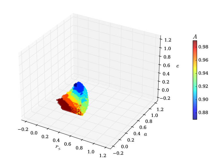
Figure 1: The space of parameters in the slowly accelerating black hole limit fixing $L=1$. The parameters of the black hole will produce four real roots obeying $r_{0}<r_{1}<0<r_{-}<r_{+}$ in (4).

The latter configuration has been referred as the slowly accelerating Kerr-Newman-AdS₄ black hole in [16]. Namely, we are interested in the space of parameters of slowly accelerating black holes with four real roots from (4) as shown in figure 1, such that the black hole parameters will satisfy $|z_{1}|<|z_{2}|$ (see (30)), a necessary condition for the formulation of the isomonodromy method.

Since the black hole does not posses an acceleration horizon, and $r_{+}$ can be interpreted as the event horizon radius, the temperature defined on the horizon is given by

$$T_{+}=\frac{1}{4\pi\alpha}\frac{\Delta_{r}^{\prime}(r_{+})}{r_{+}^{2}+a^{2}},$$ (5)

where

$$\alpha=\frac{\sqrt{\left(\Xi+\frac{a^{2}}{L^{2}}\right)\left(1-A^{2}L^{2}\Xi\right)}}{1+a^{2}A^{2}},\qquad\Xi=1-\frac{a^{2}}{L^{2}}+A^{2}\left(e^{2}+a^{2}\right),$$ (6)

where $\alpha$ can be found by analyzing the limit $M=e=0$ in (1) and removing the presence of conical deficits, and then rewriting the metric in a non-rotating frame. In this limit, the metric can be compared with a global AdS space-time, while the coordinate transformation between the space-times determines the rescaling factor of the time coordinate. We recommend [15, 16, 17] for a detailed discussion on the role of conical deficits in the thermodynamics of accelerating black holes in AdS.

II.1 The Klein-Gordon equation

In this section we will consider the conformally coupled Klein-Gordon equation on the metric (1) for massless and charged scalar fields

$$\left[\frac{1}{\sqrt{-g}}D_{\mu}\left(\sqrt{-g}g^{\mu\nu}D_{\nu}\right)-\xi R\right]\Psi=0,$$ (7)

where $D_{\mu}=\nabla_{\mu}-iqB_{\mu}$, $q$ is the charge of the field, and $\xi=1/6$ is the coupling constant in four-dimensions. The equation (7) is not separable when using the metric (1) due to the conformal factor $\Omega$. However, by performing the following conformal transformation

$$\tilde{g}_{\mu\nu}=\Omega^{2}g_{\mu\nu},$$ (8)

one can get the conformal metric

$$d\tilde{s}^{2}=-\frac{\Delta_{r}}{\rho^{2}}\left[\frac{dt}{\alpha}-a\sin^{2}\theta\frac{d\varphi}{K}\right]^{2}+\frac{\rho^{2}}{\Delta_{r}}dr^{2}+\frac{\rho^{2}}{\Delta_{\theta}}d\theta^{2}+\frac{\Delta_{\theta}\sin^{2}\theta}{\rho^{2}}\left[\frac{a\,dt}{\alpha}-(r^{2}+a^{2})\frac{d\varphi}{K}\right]^{2},$$ (9)

while the scalar field transforms as $\tilde{\Psi}=\Omega^{-1}\Psi$ in four dimensions (we refer to Appendix D in [35] for further details). The latter transformations ensure the separability of the scalar wave equation

$$\left[\frac{1}{\sqrt{-\tilde{g}}}\tilde{D}_{\mu}\left(\sqrt{-\tilde{g}}\tilde{g}^{\mu\nu}\tilde{D}_{\nu}\right)-\xi\tilde{R}\right]\tilde{\Psi}=0,$$ (10)

which in the conformally rescaled metric (9) reduces to

$$\begin{split}\biggl{\{}\frac{\partial}{\partial r}\left(\Delta_{r}\frac{\partial}{\partial r}\right)&+\frac{1}{\sin\theta}\frac{\partial}{\partial\theta}\left(\sin\theta\Delta_{\theta}\frac{\partial}{\partial\theta}\right)+\frac{\alpha^{2}(r^{2}+a^{2})^{2}}{\Delta_{r}}\left[i\frac{\partial}{\partial t}+q\Phi_{t}-\frac{q\,e\,r}{\alpha(r^{2}+a^{2})}+i\frac{a\,K}{\alpha(r^{2}+a^{2})}\frac{\partial}{\partial\varphi}\right]^{2}\\ &+\frac{\sin^{2}\theta}{\Delta_{\theta}}\left[\alpha\,a\left(\frac{\partial}{\partial t}-i\,q\Phi_{t}\right)+\frac{K}{\sin^{2}\theta}\frac{\partial}{\partial\varphi}\right]^{2}+\xi\left(\Delta_{r}^{\prime\prime}+\Delta_{\theta}^{\prime\prime}+3\cot\theta\Delta_{\theta}^{\prime}-2\Delta_{\theta}\right)\biggr{\}}\tilde{\Psi}=0.\end{split}$$ (11)

Then, by defining the following Ansatz

$$\tilde{\Psi}(t,r,\theta,\varphi)=e^{-i\omega t+im\varphi}R(r)S(\theta),$$ (12)

we obtain two second-order ODEs of the form

$$\begin{split}\frac{d}{d\theta}\left(\sin\theta\Delta_{\theta}\frac{dS}{d\theta}\right)+\biggl{\{}&-\frac{\sin^{3}\theta}{\Delta_{\theta}}\biggl{[}\alpha\,a\left(\omega+q\Phi_{t}\right)-\frac{K\,m}{\sin^{2}\theta}\biggr{]}^{2}\\ &\qquad+\xi\left(\sin\theta\Delta_{\theta}^{\prime\prime}+3\cos\theta\Delta_{\theta}^{\prime}-2\sin\theta\Delta_{\theta}\right)+\lambda\sin\theta\biggr{\}}S(\theta)=0,\end{split}$$ (13a)

$$\begin{split}\frac{d}{dr}\left(\Delta_{r}\frac{dR}{dr}\right)+\biggl{\{}\frac{\alpha^{2}(r^{2}+a^{2})^{2}}{\Delta_{r}}\left[\omega+q\Phi_{t}-\frac{q\,e\,r}{\alpha(r^{2}+a^{2})}-\frac{a\,K\,m}{\alpha(r^{2}+a^{2})}\right]^{2}+\xi\Delta_{r}^{\prime\prime}-\lambda\biggr{\}}R(r)=0,\end{split}$$ (13b)

where $\omega$ is the mode frequency, $m$ is the (magnetic) azimuthal quantum number, and $\lambda$ is the separation constant associated with the angular eigenvalue equation. These equations (13) are a particular case $\left(p=0\right)$ of those derived in [32].

II.1.1 The Angular Equation

By introducing $u=\cos\theta$, the angular equation (13a) can be rewritten as

$$\begin{split}\frac{d^{2}S}{du^{2}}+\biggl{[}\frac{1}{u+1}+\frac{1}{u-1}+\frac{1}{u-u_{0}}+\frac{1}{u-u_{1}}\biggr{]}\frac{dS}{du}&+\biggl{\{}-\frac{1}{\Delta_{u}^{2}}\left(\alpha\,a(\omega+q\Phi_{t})-\frac{K\,m}{(1-u^{2})}\right)^{2}\\ &+\xi\biggl{(}\frac{\Delta_{u}^{\prime\prime}}{\Delta_{u}}-\frac{4u\Delta_{u}^{\prime}}{(1-u^{2})\Delta_{u}}-\frac{2}{(1-u^{2})}\biggr{)}+\frac{\lambda}{(1-u^{2})\Delta_{u}}\biggr{\}}S(u)=0,\end{split}$$ (14)

with

$$\Delta_{u}=\gamma\left(u-u_{0}\right)\left(u-u_{1}\right),\qquad\gamma=\left(A^{2}e^{2}-\frac{a^{2}}{L^{2}}(1-A^{2}L^{2})\right).$$ (15)

This equation possesses five singular points located at $u=\{-1,1,u_{0},u_{1},\infty\}$, where the roots of the indicial equation, associated to the Frobenius solutions near each singular point, are given by

$$\beta^{\pm}_{-1}=\pm\frac{1}{2}\rho_{-1},\quad\beta^{\pm}_{1}=\pm\frac{1}{2}\rho_{1},\quad\beta^{\pm}_{u_{0}}=\pm\frac{1}{2}\rho_{u_{0}},\quad\beta^{\pm}_{u_{1}}=\pm\frac{1}{2}\rho_{u_{1}},\quad\beta^{\pm}_{\infty}=\frac{1}{2}\left(3\pm\rho_{\infty}\right),$$ (16)

$$\begin{split}&\rho_{-1}=\frac{K\,m}{\gamma\left(1+u_{0}\right)\left(1+u_{1}\right)},\qquad\rho_{1}=\frac{K\,m}{\gamma\left(1-u_{0}\right)\left(1-u_{1}\right)},\\ &\rho_{u_{0}}=\frac{2}{\gamma\left(u_{0}-u_{1}\right)}\left(\alpha\,a\left(\omega+q\Phi_{t}\right)-\frac{K\,m}{\left(1+u_{0}\right)\left(1-u_{0}\right)}\right),\\ &\rho_{u_{1}}=\frac{2}{\gamma\left(u_{0}-u_{1}\right)}\left(\alpha\,a\left(\omega+q\Phi_{t}\right)-\frac{K\,m}{\left(1+u_{1}\right)\left(1-u_{1}\right)}\right)\\ &\rho_{\infty}=\sqrt{9-48\xi}.\end{split}$$ (17)

To remove the conical singularity along $\theta=\pi$, we fix $K=\gamma\left(1+u_{0}\right)\left(1+u_{1}\right)$. Furthermore, by defining a new change of variables

$$w=\frac{u_{0}-u_{1}}{u_{0}+1}\frac{u+1}{u-u_{1}},$$ (18)

where the conformal moduli are

$$w_{1}=\frac{2\left(u_{0}-u_{1}\right)}{\left(1+u_{0}\right)\left(1-u_{1}\right)},\qquad w_{2}=\frac{u_{0}-u_{1}}{u_{0}+1},$$ (19)

and a s-homotopic transformation

$$S(w)=w^{\beta^{+}_{-1}}\left(w-w_{1}\right)^{\beta^{+}_{1}}\left(w-w_{2}\right)^{\beta^{-}_{\infty}}\left(w-1\right)^{\beta^{+}_{u_{0}}}y(w),$$ (20)

we can bring (14) into a Heun-like equation of the form

$$\begin{split}\frac{d^{2}y}{dw^{2}}+\biggl{(}\frac{1+\rho_{-1}}{w}+\frac{1+\rho_{1}}{w-w_{1}}&+\frac{1-\rho_{\infty}}{w-w_{2}}+\frac{1+\rho_{u_{0}}}{w-1}\biggr{)}\frac{dy}{dw}\\ &+\biggl{[}\frac{q_{1}q_{2}}{w(w-1)}-\frac{w_{1}(w_{1}-1)Q_{1}}{w(w-w_{1})(w-1)}-\frac{w_{2}(w_{2}-1)Q_{2}}{w(w-w_{2})(w-1)}\biggr{]}y(w)=0,\end{split}$$ (21)

$$q_{1}=\dfrac{1}{2}\left(\rho_{-1}+\rho_{1}+\rho_{u_{0}}+3-\rho_{\infty}-\rho_{u_{1}}\right),\qquad q_{2}=\dfrac{1}{2}\left(\rho_{-1}+\rho_{1}+\rho_{u_{0}}+3-\rho_{\infty}+\rho_{u_{1}}\right),$$ (22a)

$$\begin{gathered}Q_{1}=\frac{\hat{\lambda}}{w_{1}(w_{1}-1)}-\frac{1}{w_{1}}\biggl{[}\frac{1}{2}\left(\rho_{-1}+\rho_{1}\right)+\rho_{-1}\rho_{1}+2\xi\biggr{]}-\frac{1}{w_{1}-1}\biggl{[}\frac{1}{2}\left(\rho_{u_{0}}+\rho_{1}\right)+2\xi\biggr{]}\\ -\frac{1}{w_{1}-w_{2}}\biggl{[}\frac{1}{2}(3-\rho_{\infty})(1+\rho_{1})-\rho_{1}-6\xi\biggr{]},\end{gathered}$$ (22b)

$$\begin{gathered}Q_{2}=-\frac{1}{w_{2}}\biggl{[}\frac{1}{2}\rho_{-1}\left(1-\rho_{\infty}\right)+\frac{1}{2}\left(3-\rho_{\infty}\right)-6\xi\biggr{]}-\frac{1}{w_{2}-1}\biggl{[}\frac{1}{2}\rho_{u_{0}}\left(1-\rho_{\infty}\right)+\frac{1}{2}\left(3-\rho_{\infty}\right)-6\xi\biggr{]}\\ -\frac{1}{w_{1}-w_{2}}\biggl{[}\rho_{1}-\frac{1}{2}\left(3-\rho_{\infty}\right)\left(1+\rho_{1}\right)+6\xi\biggr{]},\end{gathered}$$ (22c)

where

$$\hat{\lambda}=\frac{\lambda}{\gamma\left(1+u_{0}\right)\left(1-u_{1}\right)}.$$ (23)

For the conformally coupled case, the critical exponent around $w=w_{2}$ is $\beta^{-}_{\infty}=1$, so the s-homotopic transformation (20) reduces the angular ODE (21) to a Heun equation, as the singularity at $w=w_{2}$ turns into a removable singularity [36]. Namely, we get

$$\frac{d^{2}y}{dw^{2}}+\biggl{(}\frac{1+\rho_{-1}}{w}+\frac{1+\rho_{1}}{w-w_{1}}+\frac{1+\rho_{u_{0}}}{w-1}\biggr{)}\frac{dy}{dw}+\biggl{[}\frac{q_{1}q_{2}}{w(w-1)}-\frac{w_{1}(w_{1}-1)Q_{1}}{w(w-w_{1})(w-1)}\biggr{]}y(w)=0,$$ (24)

where

$$q_{1}=\dfrac{1}{2}\left(\rho_{-1}+\rho_{1}+\rho_{u_{0}}+2-\rho_{u_{1}}\right),\qquad q_{2}=\dfrac{1}{2}\left(\rho_{-1}+\rho_{1}+\rho_{u_{0}}+2+\rho_{u_{1}}\right),$$ (25a)

$$\begin{gathered}Q_{1}=\frac{\hat{\lambda}}{w_{1}(w_{1}-1)}-\frac{1}{w_{1}}\biggl{[}\frac{1}{2}\left(\rho_{-1}+\rho_{1}\right)+\rho_{-1}\rho_{1}+\frac{1}{3}\biggr{]}-\frac{1}{w_{1}-1}\biggl{[}\frac{1}{2}\left(\rho_{u_{0}}+\rho_{1}\right)+\frac{1}{3}\biggr{]}.\end{gathered}$$ (25b)

II.1.2 The Radial Equation

As we have discussed in Section II.1.1, in the conformally coupled case the singularity at $w=w_{2}$ can be removed from the equation (21). Analoguously, the choiche of the charactheristic exponent around $r=\infty$ allows us to reduce the radial ODE, however, the scattering region between the event horizon and the infinity cannot be properly defined because the infinity is not longer a singularity. Bearing that in mind, we assume the coupling constant is $\xi=1/6+\delta$, then we can treat the singularity around $r=\infty$ as a regular singular point of the radial ODE instead of an apparent one. Although this choice complexifies the radial equation, the fact that the five singularities in (32) are regular singular points is paramount to introduce the method of isomonodromy and recast the boundary value problem (see Appendix A). For the numerics, $\delta$ is a small number that suits our treatment.

Equation (13b) possesses five singularities located at the root of $\Delta_{r}$ and the point at infinity. The characteristic exponents of the Frobenius solutions near to each finite singular point are defined by

$$\beta^{\pm}_{k}=\pm\frac{1}{2}\theta_{k},\qquad k=0,1,-,+,$$ (26)

and for $r=\infty$, we have

$$\beta^{\pm}_{\infty}=\frac{1}{2}\left(3\pm\theta_{\infty}\right),$$ (27)

where

$$\begin{split}&\theta_{k}=\frac{i}{2\pi T_{k}}\left(\omega+q\Phi_{t}-\frac{q\,e\,r_{k}}{\alpha(r_{k}^{2}+a^{2})}-\frac{a\,K\,m}{\alpha(r_{k}^{2}+a^{2})}\right),\\ &\theta_{\infty}=\sqrt{9-48\xi}.\end{split}$$ (28)

The radial equation can be written on the Riemann sphere by introducing a Möbius transformation

$$z=\frac{r-r_{1}}{r-r_{0}},$$ (29)

which fixes three singularities at $z=\{0,1,\infty\}$, while the two remaining singular points are situated at

$$z_{1}=\frac{r_{-}-r_{1}}{r_{-}-r_{0}},\qquad z_{2}=\frac{r_{+}-r_{1}}{r_{+}-r_{0}}.$$ (30)

Furthermore, we introduce the following s-homotopic transformation

$$R(z)=z^{\beta^{-}_{1}}(z-z_{1})^{\beta^{-}_{-}}(z-z_{2})^{\beta^{-}_{+}}(z-1)^{\beta^{-}_{\infty}}f(z),$$ (31)

which brings (13b) into the form of a Heun-like equation. Namely, a second-order ODE with five regular singular points, as we are considering the singularity located at infinity a regular singular point $\beta^{+}_{\infty}-\beta^{-}_{\infty}\notin\mathds{Z}$. Hence, the equation reads

$$\begin{split}\frac{d^{2}f}{dz^{2}}+\biggl{(}\frac{1-\theta_{1}}{z}+\frac{1-\theta_{-}}{z-z_{1}}&+\frac{1-\theta_{+}}{z-z_{2}}+\frac{1-\theta_{\infty}}{z-1}\biggr{)}\frac{df}{dz}\\ &+\biggl{[}\frac{\kappa_{1}\kappa_{2}}{z(z-1)}-\frac{z_{1}(z_{1}-1)K_{1}}{z(z-z_{1})(z-1)}-\frac{z_{2}(z_{2}-1)K_{2}}{z(z-z_{2})(z-1)}\biggr{]}f(z)=0,\end{split}$$ (32)

where

$$\kappa_{1}=\dfrac{1}{2}\left(\theta_{1}+\theta_{-}+\theta_{+}+\theta_{\infty}-3-\theta_{0}\right),\qquad\kappa_{2}=\dfrac{1}{2}\left(\theta_{1}+\theta_{-}+\theta_{+}+\theta_{\infty}-3+\theta_{0}\right),$$ (33a)

$$\begin{gathered}K_{1}=\frac{\tilde{\lambda}}{z_{1}(z_{1}-1)(r_{-}-r_{0})}-\frac{1}{z_{1}}\biggl{[}\theta_{1}\theta_{-}-\frac{1}{2}\left(\theta_{1}+\theta_{-}\right)+2\xi\biggr{]}-\frac{1}{z_{1}-1}\biggl{[}\theta_{-}+\frac{1}{2}(1-\theta_{-})(3-\theta_{\infty})-6\xi\biggr{]}\\ -\frac{1}{z_{1}-z_{2}}\biggl{[}\theta_{-}\theta_{+}-\frac{1}{2}\left(\theta_{-}+\theta_{+}\right)+2\xi\biggr{]},\end{gathered}$$ (33b)

$$\begin{gathered}K_{2}=-\frac{\tilde{\lambda}}{z_{2}(z_{2}-1)(r_{+}-r_{0})}+\frac{1}{z_{2}}\biggl{[}\frac{1}{2}(\theta_{1}+\theta_{+})-2\xi\biggr{]}-\frac{1}{z_{2}-1}\biggl{[}\theta_{+}+\frac{1}{2}(1-\theta_{+})(3-\theta_{\infty})-6\xi\biggr{]}\\ -\frac{1}{z_{2}-z_{1}}\biggl{[}\theta_{-}\theta_{+}-\frac{1}{2}(\theta_{-}+\theta_{+})+2\xi\biggr{]},\end{gathered}$$ (33c)

and the separation constant is

$$\tilde{\lambda}=\frac{L^{2}\lambda}{\left(1-A^{2}L^{2}\right)(r_{+}-r_{-})}.$$ (34)

II.1.3 Boundary Conditions

The QNMs are solutions of the eigenvalue problem relative to (13b) obeying specific boundary conditions. Namely, the scattering region is defined between $r_{+}<r<\infty$, and we impose purely ingoing wave at the outer horizon and regularity at the spatial infinity, which implies the following asymptotic behavior

$$R(r)\sim\begin{cases}(r-r_{+})^{-\theta_{+}/2},&r\rightarrow r_{+},\\ \\ r^{-(3+\theta_{\infty})/2},&r\rightarrow\infty.\end{cases}$$ (35)

In addition, for the angular equation (13a), we are interested in solutions that satisfy

$$S(w)\sim\begin{cases}w^{\rho_{-1}/2},&w\rightarrow 0\,\left(\theta\rightarrow\pi\right),\\ \\ (w-w_{1})^{\rho_{1}/2},&w\rightarrow w_{1}\,\left(\theta\rightarrow 0\right),\end{cases}$$ (36)

i.e., they do not blow up in the domain $\theta\in\left[0,\pi\right]$. Equations (24) and (32), along with the boundary conditions (35) and (36), establish the eigenvalue problem for the radial and angular system. First, we address the angular eigenvalue problem by finding the separation constant $\lambda$, and then, after substituting it into the radial ODE (13b), we compute the QNMs frequencies.

III The isomonodromic tau function of the accelerating KNAdS₄ black hole

The boundary value problem can be recast in terms of an initial value problem of an isomonodromic tau function. Namely, it turns out that the initial conditions for the Painlevé VI tau function (see [30] for the series representation of this transcendental function) solve the eigenvalue problem associated with the Heun equation as shown in [20]. Furthermore, the stability of several black holes under linear perturbations has been studied by solving numerically the set of transcendental equations, and asymptotic expansions for the QNMs frequencies have been obtained in the slowly rotating or the small black hole limit [21, 22, 26]. Other Painlevé tau functions have been introduced to study the confluent Heun equations that appear in asymptotically flat space-times [37, 24, 25]. Nonetheless, the presence of a fifth regular singular point has been only recently addressed in the context of conformal mapping of polycircular arc domains [18]. By using the definition of the isomonodromic tau function in terms of the Fredholm determinant [19], the authors implemented the tau function associated to the Fuchsian equation with five regular singular points. To our knowledge, the same type of ODEs appears in the scattering off massive scalar and fermionic fields by Kerr-Newman-(A)dS black holes in four dimensions [38, 39].

By inspecting (66), we can identify the following relations between the characteristic exponents and accessory parameters of a Fuchsian equation with five singularities and the radial ODE, as shown in Table 1.

Eq.(66)	$z_{1}$	$z_{2}$	$\theta_{0}$	$\theta_{1}$	$\theta_{2}$	$\theta_{3}$	$\theta_{\infty}$	$K_{1}$	$K_{2}$
Eq.(32)	$z_{1}$	$z_{2}$	$\theta_{1}$	$\theta_{-}$	$\theta_{+}$	$\theta_{\infty}$	$\theta_{0}$	$K_{1}$	$K_{2}$

Table 1: Map from the Heun-like equation to the radial equation parameters.

III.1 The separation constant

Since the angular second-order ODE possesses four regular singular points (24), one should expect that the separation constant can be calculated using the initial conditions for the Painlevé VI tau function [21, 22]

$$\frac{d}{dt}\log\tau_{\rm VI}\left(\rho;t\right)\biggr{|}_{t=w_{1}}=\frac{\left(\rho_{1}-1\right)\rho_{u_{0}}}{2(w_{1}-1)}+\frac{\left(\rho_{1}-1\right)\rho_{-1}}{2w_{1}}+Q_{1},$$ (37a)

$$\tau_{\rm VI}\left(\rho^{+};w_{1}\right)=0,$$ (37b)

where the monodromy arguments are given as follows:

$$\rho=\{\vartheta_{k};\sigma,\eta\}=\{\rho_{-1},\rho_{1}-1,\rho_{u_{0}},\rho_{u_{1}}+1;\sigma-1;\eta\},$$ (38)

and $\{\sigma,\eta\}$ are canonical coordinates that complete the monodromy data associated with the four-punctured Riemann sphere. Furthermore, the monodromy parameters in (37b) are related by shifts on the monodromies (38)

$$\rho^{+}=\{\vartheta_{k}^{+};\sigma^{+},\eta^{+}\}=\{\rho_{-1},\rho_{1},\rho_{u_{0}},\rho_{u_{1}};\sigma;\eta\}.$$ (39)

The second condition (37b) can be inverted for $t=w_{1}$ sufficiently close to zero, and its expansion can be computed recursively. Then, we can write the logarithmic derivative of the PVI tau function in (37a) as an analytic expansion of the accessory parameter in terms of the monodromy data and the conformal modulus (see equation (27) in [26]). Therefore, by replacing (25b), we obtain an asymptotic expansion for the separation constant. Nonetheless, we still need to impose the angular quantization condition on $\sigma$, which can be read from the boundary conditions (36). By demanding that the separation constant in the case of non-accelerating Schwarzschild-AdS₄, i.e., for $a\rightarrow 0$, $e\rightarrow 0$, and $A\rightarrow 0$, is

$$\lambda_{\ell}=\ell\left(\ell+1\right)+\frac{1}{3},$$ (40)

we can obtain the following conditions

$$\sigma=2(\ell+1),\qquad\sigma=-2\ell,\qquad\ell\geq|m|,$$ (41)

where $\ell$ is the angular momentum quantum number. While the initial conditions are valid for generic $w_{1}$, the implementation of the tau function will determine the accuracy in the computation of the angular eigenvalues. In the case of slowly accelerating black holes, we can use the series expansion of the tau function around zero [30, 31]. Choosing the first angular quantization condition and taking the slowly accelerating and slowly rotating limits, the separation constant of the accelerating Kerr-Newman-AdS₄ black hole yields

$$\begin{split}\lambda_{\omega,\ell,m}&=\ell\left(\ell+1\right)+\frac{1}{3}-2m\left(\omega+\frac{eq}{r_{+}}\right)a+2m\frac{(\omega r_{+}+eq)(r_{+}^{4}+L^{2}r_{+}^{2}+e^{2}L^{2})}{L^{2}r_{+}^{2}}a\,A\\ &+\frac{6L^{2}\left(\ell(\ell+1)+(m+1)(m-1)\right)(\omega r_{+}+eq)^{2}-r_{+}^{2}\left(6m^{2}\left(3\ell^{2}+3\ell-2\right)+6\ell^{4}+12\ell^{3}+5\ell^{2}-\ell-3\right)}{3L^{2}r_{+}^{2}(2\ell-1)(2\ell+3)}a^{2}\\ &+\biggl{[}\frac{(1-\ell(\ell+1)(3\ell^{2}+3\ell-1)-m^{2}(15\ell^{2}+15\ell-11))}{2(2\ell-1)(2\ell+3)}r_{+}^{2}\left(1+\frac{2r_{+}^{2}}{L^{2}}+\frac{r_{+}^{4}}{L^{4}}+\frac{2e^{2}}{L^{2}}+\frac{e^{4}}{r_{+}^{4}}\right)\\ &-\frac{\left(\ell(\ell+1)(3\ell^{2}+3\ell-2)+3m^{2}(9\ell^{2}+9\ell-7)\right)}{3(2\ell-1)(2\ell+3)}e^{2}\biggr{]}A^{2}+\mathcal{O}\left(a^{3},a^{2}A,aA^{2},A^{3}\right)\end{split}$$ (42)

Interestingly, the angular eigenvalues for different black solutions can be recovered by setting the rotation parameter, the charge or the acceleration to zero. In the case of non-rotating accelerating charged black holes $a\rightarrow 0$, the separation constant is

$$\begin{split}\lambda_{\ell,m}&=\ell\left(\ell+1\right)+\frac{1}{3}+\biggl{[}\frac{(1-\ell(\ell+1)(3\ell^{2}+3\ell-1)-m^{2}(15\ell^{2}+15\ell-11))}{2(2\ell-1)(2\ell+3)}r_{+}^{2}\left(1+\frac{2r_{+}^{2}}{L^{2}}+\frac{r_{+}^{4}}{L^{4}}+\frac{2e^{2}}{L^{2}}+\frac{e^{4}}{r_{+}^{4}}\right)\\ &-\frac{\left(\ell(\ell+1)(3\ell^{2}+3\ell-2)+3m^{2}(9\ell^{2}+9\ell-7)\right)}{3(2\ell-1)(2\ell+3)}e^{2}\biggr{]}A^{2}+\mathcal{O}(A^{3}),\end{split}$$ (43)

which reproduces the numerical results presented in [8]. Moreover, it reduces to the angular eigenvalues of the accelerating Schwarzschild-AdS₄, when $e\rightarrow 0$. Due to the combinatorial nature of the Nekrasov functions, the coefficients in the series expansion of the tau function are cumbersome, so that we have written the separation constant up to the second order in $A$.

III.2 Quasinormal modes

In order to find the QNMs, we need to solve the following set of transcendental equations:

$$\frac{\partial}{\partial t_{1}}\log\tau_{\mathrm{JMU}}\left(\rho;z_{1},z_{2}\right)=K_{1}+\frac{\theta_{0}(\theta_{1}-1)}{2z_{1}}+\frac{(\theta_{1}-1)(\theta_{2}-1)}{2(z_{1}-z_{2})}+\frac{(\theta_{1}-1)\theta_{3}}{2(z_{2}-1)},$$ (44a)

$$\frac{\partial}{\partial t_{2}}\log\tau_{\mathrm{JMU}}\left(\rho;z_{1},z_{2}\right)=K_{2}+\frac{\theta_{0}(\theta_{2}-1)}{2z_{2}}+\frac{(\theta_{2}-1)(\theta_{1}-1)}{2(z_{2}-z_{1})}+\frac{(\theta_{2}-1)\theta_{3}}{2(z_{2}-1)},$$ (44b)

$$\tau_{\rm JMU}\left(\rho^{+}_{1};z_{1},z_{2}\right)=0,$$ (44c)

$$\tau_{\rm JMU}\left(\rho^{+}_{2};z_{1},z_{2}\right)=0,$$ (44d)

where the monodromy data $\rho$ are defined by (70), with the critical exponents of the Heun-like equation, the conformal moduli, and the accessory parameters replaced according to Table 1. Thus, the initial conditions give an exact procedure to find $\{\omega,\sigma_{1},\sigma_{2},\eta_{1}\}$, while $\eta_{2}$ is determined using the radial quantization condition enforced by the radial boundary conditions (35). As shown in [22, 26], we require that the composite monodromy around the two singular points $r_{+}$ and $\infty$ satisfies

$$\sigma_{23}=\theta_{2}+\theta_{3}+2n,\qquad n\in\mathds{Z},$$ (45)

which imposes the following constraint on $e^{i\eta_{2}}$ to yield

$$e^{i\eta_{2}}=\frac{\sin\frac{\pi}{2}\left(\theta_{2}+\sigma_{1}+\sigma_{2}\right)\sin\frac{\pi}{2}\left(\theta_{2}-\sigma_{1}+\sigma_{2}\right)\sin\frac{\pi}{2}\left(\theta_{3}+\theta_{\infty}+\sigma_{2}\right)\sin\frac{\pi}{2}\left(\theta_{3}-\theta_{\infty}+\sigma_{2}\right)}{\sin\frac{\pi}{2}\left(\theta_{2}+\sigma_{1}-\sigma_{2}\right)\sin\frac{\pi}{2}\left(\theta_{2}-\sigma_{1}-\sigma_{2}\right)\sin\frac{\pi}{2}\left(\theta_{3}+\theta_{\infty}-\sigma_{2}\right)\sin\frac{\pi}{2}\left(\theta_{3}-\theta_{\infty}-\sigma_{2}\right)}.$$ (46)

Furthermore, the boundary value problem associated with (32) requires the computation of the separation constant using (37a). Nevertheless, because of the complexity of the set of transcendental equations, an analytical treatment is limited. Instead, we will show numerical results of the eigenfrequencies for black holes that are close to the critical acceleration, with $z_{1}\ll z_{2}\ll 1$, such that we can truncate the expansion of the operators $\mathsf{a}^{[k]},\mathsf{b}^{[k]},\mathsf{c}^{[k]},$ and $\mathsf{d}^{[k]}$ in the Fredholm determinant.

Table 2 shows the numerical values of the conformal moduli, defined as (19) and (30), for a given radius, rotation, charge, acceleration, and AdS radius. Hence, the roots of (4) are real, and the largest will correspond to the event horizon of the black hole. In addition, the tau function (83) is truncated up to order $Q=64$, because the high value of the ratio $z_{1}/z_{2}\simeq 0.8648366$ can reduce the precision of the method. In Figure 2, we solve the radial and angular ODEs using a direct integration method [41] for the eigenfrequencies in Table 3. The idea is to construct two Frobenius solutions near the horizon and spatial infinity, which satisfy continuity conditions at the matching point. As a result, correct eigenvalues $\{\omega_{n,\ell,m},\lambda_{\ell,m}\}$ will produce a set of solutions $\{f_{n,\ell,m}(z),y_{\ell,m}(w)\}$, which have the correct asymptotic behavior and are continuous everywhere, as well as their first derivatives.

$r_{+}$	$z_{1}$	$z_{2}$	$w_{1}$
$0.4$	$0.01072866$	$0.01240542$	$0.6446975$

Table 2: Conformal moduli for the following black hole parameters: $a=e=10^{-4}$, $\delta=10^{-15}$, $A=0.999$, and $L=1$.

Despite the high value of the ratio $z_{1}/z_{2}$, the radial and angular solutions for the $s$-wave and the $p$-wave modes are continuous and smooth at the matching point, serving as validation of the isomonodromic deformation method. Furthermore, in figure 3 we display the QNMs for different values of $r_{+}$ and $m$, while keeping fixed the angular momentum quantum number $\ell$ and the remaining black hole parameters. It can be observed that for $\ell=2$ and $m=\{0,1,2\}$, the modes are stable between $0.4\leq r_{+}\leq 0.49$ since the imaginary part of the frequencies remains negative. Table 4 shows the numerical values for the angular eigenvalues for the given parameters.

A thorough numerical analysis of the QNMs and the presence of superradiance is deserved, but is beyond the scope of this work, since we have merely attempted to describe the solution of the radial eigenvalue problem in terms of the isomonodromic tau function with five singularities.

Figure 2: Numerical solutions of $|f(z)|$ (left panel) and $|y(w)|$ (right panel) with $n=0,\ell=0,m=0$ (blue line) and $n=0,\ell=1,m=0$ (red line) for the parameters defined in Table 2.

$\left(\ell,m\right)$ $\omega_{n,\ell,n}$ $\sigma_{1}$ $\sigma_{2}$ $\eta_{1}$ $\lambda_{\ell,m}$ $\left(0,0\right)$ $2.406774-0.8408181i$ $2.04917+1.543151i$ $3.121017\times 10^{-11}+5.621827\times 10^{-11}i$ $1.351601+0.4316884i$ $0.2929692-5.781265\times 10^{-11}i$ $\left(1,0\right)$ $3.413521-1.588253i$ $1.970964+4.984311i$ $-1.625302\times 10^{-8}-3.852833\times 10^{-9}i$ $-2.037389+0.7255823i$ $2.115658-9.361689\times 10^{-11}i$

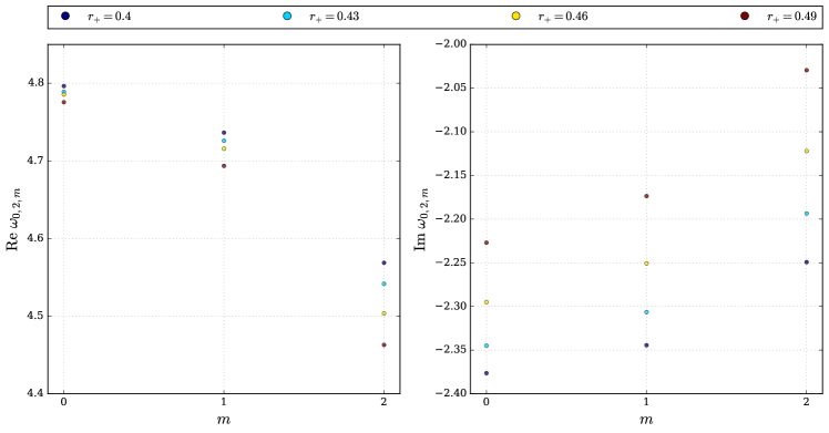
Table 3: Fundamental $(n=0)$ scalar QNMs and their associated monodromy data for the parameters in Table 2. The separation constant is found using (37a).

Figure 3: Fundamental $(n=0)$ scalar QNMs with $\ell=2$ for different values of $r_{+}$ and the azimuthal quantum number $m=\{0,1,2\}$, while keeping fixed $a=e=10^{-4}$, $\delta=10^{-15}$, $A=0.999$, and $L=1$.

$\left(\ell,m\right)$	$r_{+}$	$w_{1}$	$\lambda_{\ell,m}$
$\left(2,0\right)$	$0.4$	$0.6446975$	$5.751901-2.322604\times 10^{-10}i$
	$0.43$	$0.6902174$	$5.607453-2.32896\times 10^{-10}i$
	$0.46$	$0.7364249$	$5.425805-2.329774\times 10^{-10}i$
	$0.49$	$0.7835136$	$5.192612-2.323994\times 10^{-10}i$
$\left(2,1\right)$	$0.4$	$0.6446975$	$5.571474+1.291533\times 10^{-5}i$
	$0.43$	$0.6902174$	$5.404766+1.200439\times 10^{-5}i$
	$0.46$	$0.7364249$	$5.200931+1.098257\times 10^{-5}i$
	$0.49$	$0.7835136$	$4.93295+1.012829\times 10^{-5}i$
$\left(2,2\right)$	$0.4$	$0.6446975$	$5.051942-0.0040574i$
	$0.43$	$0.6902174$	$4.824328-0.004573267i$
	$0.46$	$0.7364249$	$4.560757-0.004855373i$
	$0.49$	$0.7835136$	$4.25052-0.004777024i$

Table 4: Angular eigenvalues $\lambda$ of the accelerating KNAdS₄ associated with Figure 3.

IV Conclusions

The conformally coupled Klein-Gordon equation for a massless scalar field in (9) separates into two second-order ODEs for the radial and angular functions. The resulting equations possess five regular singular points and can be brought into the form of a Heun-like equation (21) and (32). Nonetheless, the angular ODE can be transformed into a Heun equation (24) because the point $w=w_{2}$ is a removable singularity [36]. Therefore, the angular eigenvalue problem can be recast in terms of a set of initial conditions for the Painlevé VI tau function (37). By expanding the accessory parameter equation (37a), we have derived an asymptotic expansion (42) in the slowly accelerating and small rotation limit. This expression reproduces the results in the literature for accelerating Reissner-Nordström black holes [8].

On the other hand, the radial ODE (13b) is more intricate given that we assume the coupling constant is $\xi=1//6+\delta$, which turns the singularity at $z=1$ into a regular singular point resulting in a second-order ODE with five regular singular points (32). To this matter, we introduce to the isomonodromic deformation of the $2\times 2$ Fuchsian system with five singularities, which leads to a deformed Heun-like equation that possesses two extra apparent singularities (60). Then, by coalescing those apparent singularities with the unfixed points, one can determine the initial conditions of the Hamiltonian system (67), such that the deformed equation recovers to the radial Heun-like equation. Analogously, these initial conditions can be written in terms of an isomonodromic tau function (44) and provide the solution to the radial eigenvalue problem.

Regarding the numerical results, we use the expansion of the isomonodromic tau function for $t_{1}\ll t_{2}\ll 1$ for the computation of the scalar QNMs of a slowly accelerating KN-AdS₄ black hole. Namely, we have studied the fundamental modes for different quantum numbers $\ell$ and $m$, with given parameters $\left(r_{+},a,e,A,L\right)$, such modes have $\mathrm{Im}\,\omega<0$ suggesting the stability of black holes with $A=0.999$ and $0.4\leq r_{+}\leq 0.49$ for $\delta=10^{-15}$. The frequencies presented in Figure 3 are consistent with the photon sphere modes found in [11]. Despite the narrow space of black hole parameters that we have investigated in this work, the set of initial conditions solve the eigenvalue problem for ODEs with five regular singular points in general. It is worth mentioning that the Heun-like equation (66) appears in other problems, such as massive scalar field perturbations around Kerr-(A)dS₄ black holes, and therefore, deserves further investigation. Finally, it would be interesting to consider the extremal limit for this configuration as the resulting ODE will possess three regular and one irregular singular point, which to our knowledge has not been explored in the literature yet.

Appendix A The isomonodromic deformation approach

We consider the following Fuchsian linear system

$$\frac{d\Phi}{dz}=A(z)\Phi,\qquad z\in\mathds{C},$$ (47)

where $\Phi(z)$ is the $2\times 2$ fundamental matrix of solutions defined in the complex plane

$$\Phi(z)=\begin{pmatrix}y_{1}(z)&w_{1}(z)\\ y_{2}(z)&w_{2}(z)\\ \end{pmatrix},$$ (48)

and $A(z)$ is a $2\times 2$ matrix given by a partial fraction expansion of the form:

$$A(z)=\frac{A_{0}}{z}+\frac{A_{1}}{z-t_{1}}+\frac{A_{2}}{z-t_{2}}+\frac{A_{3}}{z-1},$$ (49)

where the residue matrices $A_{i},i=\{0,1,2,3\}$ do not depend on $z$. Furthermore, since the point at infinity is a regular singular point, we find that

$$A_{\infty}=-\left(A_{0}+A_{1}+A_{2}+A_{3}\right),$$ (50)

and, as a consequence of the isomonodromy condition, the matrix coefficients $A_{k}$ satisfy the Schlesinger system:

$$\frac{\partial A_{\ell}}{\partial t_{k}}=\frac{\left[A_{k},A_{\ell}\right]}{t_{k}-t_{\ell}}\quad\mathrm{for}\quad k\neq\ell,\quad\mathrm{and}\quad\frac{\partial A_{k}}{\partial t_{k}}=-\sum_{\ell\neq k}\frac{\left[A_{k},A_{\ell}\right]}{t_{k}-t_{\ell}},$$ (51)

which implies that $A_{\infty}=\mathrm{const}$, and using the freedom of global conjugation, one may assume

$$A_{\infty}=\begin{pmatrix}\kappa_{1}&0\\ 0&\kappa_{2}\\ \end{pmatrix}.$$ (52)

Then the entry $\left[A(z)\right]_{12}$ of the matrix $A(z)$ is given by

$$\left[A(z)\right]_{12}=\frac{k(z-\lambda_{1})(z-\lambda_{2})}{z(z-t_{1})(z-t_{2})(z-1)},$$ (53)

with some constant $k\in\mathds{C}$ and $\{\lambda_{1},\lambda_{2}\}$ are a set of zeros in the complex plane.

The Fuchsian system (47) has an associated second-order ordinary differential equation for the first row of the fundamental matrix

$$y^{\prime\prime}_{j}(z)-\left(\operatorname{Tr}A+\frac{\left[A^{\prime}(z)\right]_{12}}{\left[A(z)\right]_{12}}\right)y^{\prime}_{j}(z)+\left(\det A-\left[A^{\prime}(z)\right]_{11}+\left[A(z)\right]_{11}\frac{\left[A^{\prime}(z)\right]_{12}}{\left[A(z)\right]_{12}}\right)y_{j}(z)=0,\quad j=\{1,2\},$$ (54)

where the prime denotes a derivative with respect to $z$. By introducing (64), (50) and (53), the equation reduces to

$$y^{\prime\prime}(z)+p(z)y^{\prime}+q(z)y(z)=0,$$ (55)

with

$$p(z)=\frac{1-\operatorname{Tr}A_{0}}{z}+\frac{1-\operatorname{Tr}A_{1}}{z-t_{1}}+\frac{1-\operatorname{Tr}A_{2}}{z-t_{2}}+\frac{1-\operatorname{Tr}A_{3}}{z-1}-\frac{1}{z-\lambda_{1}}-\frac{1}{z-\lambda_{2}},$$ (56)

and

$$\begin{gathered}q(z)=\frac{\det A_{0}}{z^{2}}+\frac{\det A_{1}}{(z-t_{1})^{2}}+\frac{\det A_{2}}{(z-t_{2})^{2}}+\frac{\det A_{3}}{(z-1)^{2}}+\frac{\kappa}{z(z-1)}-\frac{t_{1}(t_{1}-1)\mathcal{K}_{1}}{z(z-t_{1})(z-1)}-\frac{t_{2}(t_{2}-1)\mathcal{K}_{2}}{z(z-t_{2})(z-1)}\\ +\frac{\left[A_{\infty}\right]_{11}}{z(z-1)}+\frac{\lambda_{1}(\lambda_{1}-1)\mu_{1}}{z(z-\lambda_{1})(z-1)}+\frac{\lambda_{2}(\lambda_{2}-1)\mu_{2}}{z(z-\lambda_{2})(z-1)},\end{gathered}$$ (57)

where

$$\kappa=\det A_{\infty}-\det A_{0}-\det A_{1}-\det A_{2}-\det A_{3},$$ (58a)

$$\mu_{1}=\frac{\left[A_{0}\right]_{11}}{\lambda_{1}}+\frac{\left[A_{1}\right]_{11}}{\lambda_{1}-t_{1}}+\frac{\left[A_{2}\right]_{11}}{\lambda_{1}-t_{2}}+\frac{\left[A_{3}\right]_{11}}{\lambda_{1}-1},$$ (58b)

$$\mu_{2}=\frac{\left[A_{0}\right]_{11}}{\lambda_{2}}+\frac{\left[A_{1}\right]_{11}}{\lambda_{2}-t_{1}}+\frac{\left[A_{2}\right]_{11}}{\lambda_{2}-t_{2}}+\frac{\left[A_{3}\right]_{11}}{\lambda_{2}-1},$$ (58c)

$$\begin{split}\mathcal{K}_{1}=&\frac{1}{t_{1}}\operatorname{Tr}(A_{0}A_{1})+\frac{1}{t_{1}-t_{2}}\operatorname{Tr}(A_{1}A_{2})+\frac{1}{t_{1}-1}\operatorname{Tr}(A_{1}A_{3})-\frac{1}{t_{1}}\operatorname{Tr}A_{0}\operatorname{Tr}A_{1}-\frac{1}{t_{1}-t_{2}}\operatorname{Tr}A_{1}\operatorname{Tr}A_{2}\\ &-\frac{1}{t_{1}-1}\operatorname{Tr}A_{1}\operatorname{Tr}A_{3}+\frac{\left[A_{0}\right]_{11}+\left[A_{1}\right]_{11}}{t_{1}}+\frac{\left[A_{1}\right]_{11}+\left[A_{2}\right]_{11}}{t_{1}-t_{2}}+\frac{\left[A_{1}\right]_{11}+\left[A_{3}\right]_{11}}{t_{1}-1}-\frac{\left[A_{1}\right]_{11}}{t_{1}-\lambda_{1}}-\frac{\left[A_{1}\right]_{11}}{t_{1}-\lambda_{2}},\end{split}$$ (58d)

$$\begin{split}\mathcal{K}_{2}=&\frac{1}{t_{2}}\operatorname{Tr}(A_{0}A_{2})+\frac{1}{t_{2}-t_{1}}\operatorname{Tr}(A_{2}A_{1})+\frac{1}{t_{2}-1}\operatorname{Tr}(A_{2}A_{3})-\frac{1}{t_{2}}\operatorname{Tr}A_{0}\operatorname{Tr}A_{2}-\frac{1}{t_{2}-t_{1}}\operatorname{Tr}A_{2}\operatorname{Tr}A_{1}\\ &-\frac{1}{t_{2}-1}\operatorname{Tr}A_{2}\operatorname{Tr}A_{3}+\frac{\left[A_{0}\right]_{11}+\left[A_{2}\right]_{11}}{t_{2}}+\frac{\left[A_{1}\right]_{11}+\left[A_{2}\right]_{11}}{t_{2}-t_{1}}+\frac{\left[A_{2}\right]_{11}+\left[A_{3}\right]_{11}}{t_{2}-1}-\frac{\left[A_{2}\right]_{11}}{t_{2}-\lambda_{1}}-\frac{\left[A_{2}\right]_{11}}{t_{2}-\lambda_{2}}.\end{split}$$ (58e)

In addition, we choose the following properties for the residue matrices

$$\operatorname{Tr}{A_{k}}=\vartheta_{k},\qquad\det A_{k}=0,\qquad k=\{0,1,2,3\},$$ (59)

which bring (55) into the form

$$\begin{split}y^{\prime\prime}(z)+\biggl{[}\frac{1-\vartheta_{0}}{z}&+\frac{1-\vartheta_{1}}{z-t_{1}}+\frac{1-\vartheta_{2}}{z-t_{2}}+\frac{1-\vartheta_{3}}{z-1}-\frac{1}{z-\lambda_{1}}-\frac{1}{z-\lambda_{2}}\biggr{]}y^{\prime}(z)\\ &+\biggl{(}\frac{\kappa_{1}(1+\kappa_{2})}{z(z-1)}-\frac{t_{1}(t_{1}-1)\mathcal{K}_{1}}{z(z-t_{1})(z-1)}-\frac{t_{2}(t_{2}-1)\mathcal{K}_{2}}{z(z-t_{2})(z-1)}\\ &\qquad\qquad\qquad+\frac{\lambda_{1}(\lambda_{1}-1)\mu_{1}}{z(z-\lambda_{1})(z-1)}+\frac{\lambda_{2}(\lambda_{2}-1)\mu_{2}}{z(z-\lambda_{2})(z-1)}\biggr{)}y(z)=0.\end{split}$$ (60)

One can show that the singular points at $z=\lambda_{j}$ are apparent singularities, as the characteristic exponents are integers, and therefore the monodromies around these points are trivial. The latter impose an algebraic relation between $\mathcal{K}_{j}$, $\mu_{j}$, $\lambda_{j}$ and $t_{j}$,

$$\begin{split}\mathcal{K}_{1}=&-\frac{\lambda_{1}(\lambda_{1}-t_{1})(\lambda_{1}-t_{2})(\lambda_{1}-1)(\lambda_{2}-t_{1})}{t_{1}(t_{1}-t_{2})(t_{1}-1)(\lambda_{1}-\lambda_{2})}\biggl{[}\mu_{1}^{2}-\left(\frac{\vartheta_{0}}{\lambda_{1}}+\frac{\vartheta_{1}-1}{\lambda_{1}-t_{1}}+\frac{\vartheta_{2}}{\lambda_{1}-t_{2}}+\frac{\vartheta_{3}}{\lambda_{1}-1}\right)\mu_{1}\\ &+\frac{\kappa_{1}(1+\kappa_{2})(\lambda_{1}-\lambda_{2})}{\lambda_{1}(\lambda_{1}-t_{2})(\lambda_{1}-1)}\biggr{]}-\frac{\lambda_{2}(\lambda_{2}-t_{1})(\lambda_{2}-t_{2})(\lambda_{2}-1)(\lambda_{1}-t_{1})}{t_{1}(t_{1}-t_{2})(t_{1}-1)(\lambda_{2}-\lambda_{1})}\biggl{[}\mu_{2}^{2}\\ &-\left(\frac{\vartheta_{0}}{\lambda_{2}}+\frac{\vartheta_{1}-1}{\lambda_{2}-t_{1}}+\frac{\vartheta_{2}}{\lambda_{2}-t_{2}}+\frac{\vartheta_{3}}{\lambda_{2}-1}\right)\mu_{2}\biggr{]},\end{split}$$ (61a)

$$\begin{split}\mathcal{K}_{2}=&-\frac{\lambda_{2}(\lambda_{2}-t_{1})(\lambda_{2}-t_{2})(\lambda_{2}-1)(\lambda_{1}-t_{2})}{t_{2}(t_{2}-t_{1})(t_{2}-1)(\lambda_{2}-\lambda_{1})}\biggl{[}\mu_{2}^{2}-\left(\frac{\vartheta_{0}}{\lambda_{2}}+\frac{\vartheta_{1}}{\lambda_{2}-t_{1}}+\frac{\vartheta_{2}-1}{\lambda_{2}-t_{2}}+\frac{\vartheta_{3}}{\lambda_{2}-1}\right)\mu_{2}\\ &+\frac{\kappa_{1}(1+\kappa_{2})(\lambda_{2}-\lambda_{1})}{\lambda_{2}(\lambda_{2}-t_{1})(\lambda_{2}-1)}\biggr{]}-\frac{\lambda_{1}(\lambda_{1}-t_{1})(\lambda_{1}-t_{2})(\lambda_{1}-1)(\lambda_{2}-t_{2})}{t_{2}(t_{2}-t_{1})(t_{2}-1)(\lambda_{1}-\lambda_{2})}\biggl{[}\mu_{1}^{2}\\ &-\left(\frac{\vartheta_{0}}{\lambda_{1}}+\frac{\vartheta_{1}}{\lambda_{1}-t_{1}}+\frac{\vartheta_{2}-1}{\lambda_{1}-t_{2}}+\frac{\vartheta_{3}}{\lambda_{1}-1}\right)\mu_{1}\biggr{]}.\end{split}$$ (61b)

Okamoto showed that the isomonodromic deformation equations (51) of the Fuchsian system (47) can be obtained from the Hamiltonian system [42]:

$$\frac{\partial\lambda_{i}}{\partial t_{j}}=\frac{\partial\mathcal{K}_{j}}{\partial\mu_{i}},\qquad\frac{\partial\mu_{i}}{\partial t_{j}}=-\frac{\partial\mathcal{K}_{j}}{\partial\lambda_{i}},\qquad i,j=\{1,2\},$$ (62)

where $(\lambda_{j},\mu_{j})$ are canonical variables, $\mathcal{K}_{j}$ is the Hamiltonian. Such dynamical system (62) is known as the two-dimensional Garnier system, denoted by $G_{2}(\mathbf{\vartheta}),\,\,\,\mathbf{\vartheta}=\{\vartheta_{0},\vartheta_{1},\vartheta_{2},\vartheta_{3},\vartheta_{\infty}\}$, and is completely integrable. Furthermore, we can introduce an isomonodromic Jimbo-Miwa-Ueno (JMU) tau function, defined by

$$\frac{\partial}{\partial t_{k}}\log\tau_{\mathrm{JMU}}=\sum_{\ell=0,\ell\neq k}^{3}\frac{1}{t_{k}-t_{\ell}}\operatorname{Tr}A_{k}A_{\ell},\quad\quad k=\{1,2\},$$ (63)

which is a closed $1$-form provided that the Schlesinger equations (51) are satisfied. The definition (63) assumes that residue matrices are traceless $A_{k}\in sl(2,\mathbb{C})$, which is in contrast with our choice (59). In principle those residue matrices will correspond to a different Fuchsian system (47), but one can check that the by performing the following transformation $A^{\prime}_{k}=A_{k}-\tfrac{1}{2}\vartheta_{k}\mathds{1}$, the solutions of Fuchsian systems of traceless and not traceless residue matrices are related by multiplicative factors. Namely, the isomonodromic tau functions are related by

$$\frac{\partial}{\partial t_{k}}\log\tau^{\prime}_{\mathrm{JMU}}=\frac{\partial}{\partial t_{k}}\log\tau_{\mathrm{JMU}}-\frac{1}{2}\sum_{\ell=0,\ell\neq k}^{3}\frac{\vartheta_{k}\vartheta_{\ell}}{t_{k}-t_{\ell}},\quad\quad k=\{1,2\}.$$ (64)

Thus by replacing (64) into eqs. 58d and 58e, as well as equating to their corresponding Hamiltoninian in (61), we obtain

$$\begin{split}\frac{\partial}{\partial t_{1}}\log\tau^{\prime}_{\mathrm{JMU}}=&\frac{\vartheta_{0}\vartheta_{1}}{2t_{1}}+\frac{\vartheta_{1}\vartheta_{2}}{2(t_{1}-t_{2})}+\frac{\vartheta_{1}\vartheta_{3}}{2(t_{1}-1)}-\frac{\left[A_{0}\right]_{11}+\left[A_{1}\right]_{11}}{t_{1}}\\ &-\frac{\left[A_{1}\right]_{11}+\left[A_{2}\right]_{11}}{t_{1}-t_{2}}-\frac{\left[A_{1}\right]_{11}+\left[A_{3}\right]_{11}}{t_{1}-1}+\frac{\left[A_{1}\right]_{11}}{t_{1}-\lambda_{1}}+\frac{\left[A_{1}\right]_{11}}{t_{1}-\lambda_{2}}+\mathcal{K}_{1},\end{split}$$ (65a)

$$\begin{split}\frac{\partial}{\partial t_{2}}\log\tau^{\prime}_{\mathrm{JMU}}=&\frac{\vartheta_{0}\vartheta_{2}}{2t_{2}}+\frac{\vartheta_{2}\vartheta_{1}}{2(t_{2}-t_{1})}+\frac{\vartheta_{2}\vartheta_{3}}{2(t_{2}-1)}-\frac{\left[A_{0}\right]_{11}+\left[A_{2}\right]_{11}}{t_{2}}\\ &-\frac{\left[A_{1}\right]_{11}+\left[A_{2}\right]_{11}}{t_{2}-t_{1}}-\frac{\left[A_{2}\right]_{11}+\left[A_{3}\right]_{11}}{t_{2}-1}+\frac{\left[A_{2}\right]_{11}}{t_{2}-\lambda_{1}}+\frac{\left[A_{2}\right]_{11}}{t_{2}-\lambda_{2}}+\mathcal{K}_{2}.\end{split}$$ (65b)

Given the isomonodromic tau function for (65), we can establish the Riemann-Hilbert map to relate the accessory parameters of the Fuchsian ODEs to the monodromy data. One can show that by setting initial conditions to the Hamiltonian system, the deformed equation (60) recovers a Heun-like equation with five singularities of the form

$$\begin{split}\frac{d^{2}y}{dz^{2}}+\biggl{(}\frac{1-\theta_{0}}{z}+\frac{1-\theta_{1}}{z-z_{1}}&+\frac{1-\theta_{2}}{z-z_{2}}+\frac{1-\theta_{3}}{z-1}\biggr{)}\frac{dy}{dz}\\ &+\biggl{[}\frac{\kappa_{+}\kappa_{-}}{z(z-1)}-\frac{z_{1}(z_{1}-1)K_{1}}{z(z-z_{1})(z-1)}-\frac{z_{2}(z_{2}-1)K_{2}}{z(z-z_{2})(z-1)}\biggr{]}y(z)=0,\end{split}$$ (66)

where each apparent singularity has merged with one regular singular point. Namely, we require the following initial conditions

$$\begin{split}\lambda_{1}(t_{1}=z_{1},t_{2}=z_{2})=z_{1},\quad\mu_{1}(t_{1}=z_{1},t_{2}=z_{2})=\frac{K_{1}}{1-\theta_{1}},\\ \lambda_{2}(t_{1}=z_{1},t_{2}=z_{2})=z_{2},\quad\mu_{2}(t_{1}=z_{1},t_{2}=z_{2})=\frac{K_{2}}{1-\theta_{2}},\end{split}$$ (67)

while the local monodromies will change as follows

$$\vartheta_{0}=\theta_{0},\quad\vartheta_{1}=\theta_{1}-1,\quad\vartheta_{2}=\theta_{2}-1,\quad\vartheta_{3}=\theta_{3},\quad\vartheta_{\infty}=\theta_{\infty}+1.$$ (68)

The conditions (67) yield a well-posed initial value problem for the Garnier system (62). As it has been shown in [18], these conditions can be rewritten in terms of the isomonodromic tau function. In turn, the initial conditions for $\left(\mu_{k}(\{z_{k}\}),\lambda_{k}(\{z_{k}\})\right)$ will be related to the logarithmic derivative and a zero of the tau function $\tau_{\rm JMU}$ with given monodromy data. Namely, we have

$$\frac{\partial}{\partial t_{k}}\log\tau_{\mathrm{JMU}}\left(\rho;\{z_{k}\}\right)=K_{k}+\frac{\vartheta_{0}\vartheta_{k}}{2t_{k}}+\sum^{2}_{l\neq k}\frac{\vartheta_{k}\vartheta_{l}}{2(t_{k}-t_{l})}+\frac{\vartheta_{k}\vartheta_{3}}{2(t_{k}-1)},\qquad k=\{1,2\}$$ (69a)

$$\tau_{\rm JMU}\left(\rho^{+}_{k};\{z_{k}\}\right)=0,$$ (69b)

where the monodromy arguments $\rho$ and $\rho_{k}^{+}$ are related by shifts:

$$\rho=\{\vartheta;\sigma_{k};\eta_{k}\}=\{\theta_{0},\theta_{1}-1,\theta_{2}-1,\theta_{3},\theta_{\infty}+1;\sigma_{1}-1,\sigma_{2}-1;\eta_{1},\eta_{2}\},$$ (70a)

$$\rho_{1}^{+}=\{\vartheta^{+};\sigma^{+}_{k};\eta^{+}_{k}\}=\{\theta_{0},\theta_{1},\theta_{2}-1,\theta_{3},\theta_{\infty};\sigma_{1},\sigma_{2};\eta_{1},\eta_{2}\},$$ (70b)

$$\rho_{2}^{+}=\{\vartheta^{+};\sigma^{+}_{k};\eta^{+}_{k}\}=\{\theta_{0},\theta_{1}-1,\theta_{2},\theta_{3},\theta_{\infty};\sigma_{1}-1,\sigma_{2};\eta_{1},\eta_{2}\},$$ (70c)

where the set of transcendental equations (69) supplemented with (70) will solve the boundary value problem for the radial ODE (32).

Appendix B The isomonodromic tau-function with five singularities

The Jimbo-Miwa-Ueno isomonodromic tau function $\tau_{\rm JMU}(t)$ admits a block determinant representation

$$\tau_{\rm JMU}(t)=\Upsilon(t)\cdot\det\left(\mathds{1}-\mathrm{K}\right),$$ (71)

where the operator $\mathrm{K}$ is

$$\mathrm{K}=\begin{pmatrix}0&\mathsf{a}^{[2]}&\mathsf{b}^{[2]}&0&0&0&\ldots&0&0\\ \mathsf{d}^{[1]}&0&0&0&0&0&\dots&0&0\\ 0&0&0&\mathsf{a}^{[3]}&\mathsf{b}^{[3]}&0&\ldots&0&0\\ 0&\mathsf{c}^{[2]}&\mathsf{d}^{[2]}&0&0&0&\ldots&0&0\\ 0&0&0&0&0&\mathsf{a}^{[4]}&\ldots&0&0\\ 0&0&0&\mathsf{c}^{[3]}&\mathsf{d}^{[3]}&0&\ldots&0&0\\ \vdots&\vdots&\vdots&\vdots&\vdots&\vdots&\ddots&\vdots&\vdots\\ 0&0&0&0&0&0&\ldots&0&\mathsf{a}^{[n-2]}\\ 0&0&0&0&0&0&\ldots&\mathsf{d}^{[n-3]}&0\\ \end{pmatrix},$$ (72)

$n$ corresponds to the number of regular singular points on $\mathds{P}^{1}$, and $\Upsilon(t)$ is an analytic function of the positions of the remaining singular points that cannot be fixed by a Möbius transformation $t=\{t_{1},\ldots,t_{n-3}\}$.

The operators $\mathsf{a}^{[k]},\mathsf{b}^{[k]},\mathsf{c}^{[k]},\mathsf{d}^{[k]}$ are Cauchy-Plemelj operators $\mathcal{P}_{\bigoplus}:\mathcal{H}\rightarrow\mathcal{H}$ of the form:

$$\begin{split}\left(\mathsf{a}^{[k]}g\right)(z)=\oint_{\mathcal{C}^{[k-1]}}\frac{dz^{\prime}}{2\pi i}\mathsf{a}^{[k]}(z,z^{\prime})g(z^{\prime}),\qquad\left(\mathsf{b}^{[k]}g\right)(z)=\oint_{\mathcal{C}^{[k]}}\frac{dz^{\prime}}{2\pi i}\mathsf{b}^{[k]}(z,z^{\prime})g(z^{\prime}),\\ \left(\mathsf{c}^{[k]}g\right)(z)=\oint_{\mathcal{C}^{[k-1]}}\frac{dz^{\prime}}{2\pi i}\mathsf{c}^{[k]}(z,z^{\prime})g(z^{\prime}),\qquad\left(\mathsf{d}^{[k]}g\right)(z)=\oint_{\mathcal{C}^{[k]}}\frac{dz^{\prime}}{2\pi i}\mathsf{d}^{[k]}(z,z^{\prime})g(z^{\prime}),\end{split}$$ (73)

where the integral kernels of the 3-point projection operators can be expanded in a Fourier basis converging inside the trinion $\mathcal{T}^{[k]}$,

$$\mathsf{a}^{[k]}(z,z^{\prime})=\frac{\Psi^{[k]}_{+}(z)\Psi^{[k]}_{+}(z^{\prime})^{-1}-\mathds{1}}{z-z^{\prime}}=\sum_{p,q=1}^{\infty}\left(\mathsf{A}^{[k]}\right)^{p}_{q}z^{p-1}z^{\prime}\,{}^{q-1},\qquad z\in\mathcal{C}^{[k-1]},$$ (74a)

$$\mathsf{b}^{[k]}(z,z^{\prime})=-\frac{\Psi^{[k]}_{+}(z)\Psi^{[k]}_{+}(z^{\prime})^{-1}}{z-z^{\prime}}=\sum_{p,q=1}^{\infty}\left(\mathsf{B}^{[k]}\right)^{p}_{q}z^{p-1}z^{\prime}\,{}^{-q},\qquad z\in\mathcal{C}^{[k-1]},$$ (74b)

$$\mathsf{c}^{[k]}(z,z^{\prime})=\frac{\Psi^{[k]}_{+}(z)\Psi^{[k]}_{+}(z^{\prime})^{-1}}{z-z^{\prime}}=\sum_{p,q=1}^{\infty}\left(\mathsf{C}^{[k]}\right)^{p}_{q}z^{-p}z^{\prime}\,{}^{q-1},\qquad z\in\mathcal{C}^{[k]},$$ (74c)

$$\mathsf{d}^{[k]}(z,z^{\prime})=\frac{\mathds{1}-\Psi^{[k]}_{+}(z)\Psi^{[k]}_{+}(z^{\prime})^{-1}}{z-z^{\prime}}=\sum_{p,q=1}^{\infty}\left(\mathsf{D}^{[k]}\right)^{p}_{q}z^{-p}z^{\prime}\,{}^{-q},\qquad z\in\mathcal{C}^{[k]},$$ (74d)

with the Fourier coefficients (74) given by semi-infinite matrices whose $N\times N$ blocks are determined by

$$\left(\mathsf{A}^{[k]}\right)^{p}_{q}=t_{k}^{\frac{1}{2}\sigma_{k-1}\bm{\sigma}_{3}}\left(\sum_{r=1}^{p}\left[\Psi^{[k]}\,{}^{-1}\right]_{q+r-1}\left[\Psi^{[k]}\right]_{p-r}t_{k}^{-p-q+1}\right)t_{k}^{-\frac{1}{2}\sigma_{k-1}\bm{\sigma}_{3}},$$ (75a)

$$\left(\mathsf{B}^{[k]}\right)^{p}_{q}=\kappa_{k}^{\frac{1}{2}\bm{\sigma}_{3}}t_{k}^{\frac{1}{2}\sigma_{k}\bm{\sigma}_{3}}\left(\sum_{r=1}^{\mathrm{min}(p,q)}\left[\tilde{\Psi}^{[k]}\,{}^{-1}\right]_{q-r}\bm{\mathrm{G}}_{k}^{-1}\left[\Psi^{[k]}\right]_{p-r}t_{k}^{-p+q}\right)t_{k}^{-\frac{1}{2}\sigma_{k-1}\bm{\sigma}_{3}},$$ (75b)

$$\left(\mathsf{C}^{[k]}\right)^{p}_{q}=t_{k}^{\frac{1}{2}\sigma_{k}\bm{\sigma}_{3}}\left(\sum_{r=1}^{\mathrm{min}(p,q)}\left[\Psi^{[k]}\,{}^{-1}\right]_{q-r}\bm{\mathrm{G}}_{k}\left[\tilde{\Psi}^{[k]}\right]_{p-r}t_{k}^{p-q}\right)t_{k}^{\frac{1}{2}\sigma_{k-1}\bm{\sigma}_{3}}\kappa_{k}^{\frac{1}{2}\bm{\sigma}_{3}},$$ (75c)

$$\left(\mathsf{D}^{[k]}\right)^{p}_{q}=\kappa_{k}^{\frac{1}{2}\bm{\sigma}_{3}}t_{k}^{\frac{1}{2}\sigma_{k}\bm{\sigma}_{3}}\left(\sum_{r=1}^{p}\left[\tilde{\Psi}^{[k]}\,{}^{-1}\right]_{q+r-1}\left[\tilde{\Psi}^{[k]}\right]_{p-r}t_{k}^{p+q-1}\right)t_{k}^{-\frac{1}{2}\sigma_{k}\bm{\sigma}_{3}}\kappa_{k}^{-\frac{1}{2}\bm{\sigma}_{3}}.$$ (75d)

where the matrix functions $\Psi^{[k]}$ and $\tilde{\Psi}^{[k]}$ solve the Riemann-Hilbert Problem associated to $3$-point Fuchsian systems with prescribed monodromy. For $|t_{1}|\ll|t_{2}|\ll\cdots\ll 1$, the tau function can be expanded by truncating the kernels in the expansion of $\mathsf{a}^{[k]},\mathsf{b}^{[k]},\mathsf{c}^{[k]},\mathsf{d}^{[k]}$ up to order $Q\in\mathds{Z}_{>0}$, such that the Fourier coefficients (75) satisfy $p+q\leq Q$, denoted by $NQ\times NQ$-dimensional blocks (see [19] for an explicit representation of the matrices). The latter gives the asymptotic expansion of $\tau_{\rm JMU}(t)$ to arbitrary finite order $Q$. Now, let us expand the parametrices

$$\begin{split}&\Psi(\sigma_{k-1},\vartheta_{k},\sigma_{k};z/t_{k})=\sum_{n=0}^{\infty}\left[\Psi^{[k]}\right]_{n}\left(\frac{z}{t_{k}}\right)^{n},\\ &\Psi(-\sigma_{k},\vartheta_{k},\sigma_{k-1};t_{k}/z)=\sum_{n=0}^{\infty}\left[\tilde{\Psi}^{[k]}\right]_{n}\left(\frac{t_{k}}{z}\right)^{n},\end{split}$$ (76)

with $\bigl{[}\Psi^{[k]}\bigr{]}_{0}=\bigl{[}\tilde{\Psi}^{[k]}\bigr{]}_{0}=\mathds{1}$. In particular, for $N=2$, $3$-point RHPs can be solved in terms of Gauss hypergeometric functions

$$\Psi(\alpha_{1},\alpha_{2},\alpha_{3};z)=\begin{pmatrix}\phi(\alpha_{1},\alpha_{2},\alpha_{3};z)&\chi(\alpha_{1},\alpha_{2},\alpha_{3};z)\\ \chi(-\alpha_{1},\alpha_{2},\alpha_{3};z)&\phi(-\alpha_{1},\alpha_{2},\alpha_{3};z)\\ \end{pmatrix},$$ (77)

where

$$\begin{split}\phi(\alpha_{1},\alpha_{2},\alpha_{3};z)&=\,_{2}F_{1}\left(\frac{1}{2}(\alpha_{1}-\alpha_{2}+\alpha_{3}),\frac{1}{2}(\alpha_{1}-\alpha_{2}-\alpha_{3}),\alpha_{1};z\right),\\ \chi(\alpha_{1},\alpha_{2},\alpha_{3};z)&=\frac{\alpha_{3}^{2}-(\alpha_{2}-\alpha_{1})^{2}}{4\alpha_{1}(\alpha_{1}+1)}z\,_{2}F_{1}\left(1+\frac{1}{2}(\alpha_{1}-\alpha_{2}+\alpha_{3}),1+\frac{1}{2}(\alpha_{1}-\alpha_{2}-\alpha_{3}),2+\alpha_{1};z\right)\end{split}$$ (78)

and $\bm{\mathrm{G}}_{k}$ and $\kappa_{k}$ are given by

$$\bm{\mathrm{G}}_{k}=\frac{1}{2\sigma_{k}}\begin{pmatrix}\sigma_{k-1}+\vartheta_{k}+\sigma_{k}&\sigma_{k-1}+\vartheta_{k}-\sigma_{k}\\ \sigma_{k-1}-\vartheta_{k}-\sigma_{k}&\sigma_{k-1}-\vartheta_{k}+\sigma_{k}\\ \end{pmatrix},$$ (79)

$$\begin{split}\kappa_{k}=&\,e^{i\eta_{k}}\frac{\Gamma^{2}\left(1-\sigma_{k}\right)}{\Gamma^{2}\left(1+\sigma_{k}\right)}\frac{\Gamma\left(1+\frac{1}{2}(\vartheta_{k}+\sigma_{k-1}+\sigma_{k})\right)\Gamma\left(1+\frac{1}{2}(\vartheta_{k}-\sigma_{k-1}+\sigma_{k})\right)}{\Gamma\left(1+\frac{1}{2}(\vartheta_{k}+\sigma_{k-1}-\sigma_{k})\right)\Gamma\left(1+\frac{1}{2}(\vartheta_{k}-\sigma_{k-1}-\sigma_{k})\right)}\\ &\times\frac{\Gamma\left(1+\frac{1}{2}(\vartheta_{k+1}+\sigma_{k+1}+\sigma_{k})\right)\Gamma\left(1+\frac{1}{2}(\vartheta_{k+1}-\sigma_{k+1}+\sigma_{k})\right)}{\Gamma\left(1+\frac{1}{2}(\vartheta_{k+1}+\sigma_{k+1}-\sigma_{k})\right)\Gamma\left(1+\frac{1}{2}(\vartheta_{k+1}-\sigma_{k+1}-\sigma_{k})\right)}.\end{split}$$ (80)

Furthermore, for $n=5$, the determinant reduces to

$$\mathrm{K}=\begin{pmatrix}0&\mathsf{a}^{[2]}&\mathsf{b}^{[2]}&0\\ \mathsf{d}^{[1]}&0&0&0\\ 0&0&0&\mathsf{a}^{[3]}\\ 0&\mathsf{c}^{[2]}&\mathsf{d}^{[2]}&0\end{pmatrix},$$ (81)

satisfying the decomposition of the five-punctured Riemann sphere into three trinions:

$$\begin{split}&\mathcal{T}^{[1]}:\sigma_{0}=\vartheta_{0},\vartheta_{1},\sigma_{1},\eta_{1},t_{1};\\ &\mathcal{T}^{[2]}:\sigma_{1},\vartheta_{2},\sigma_{2},\eta_{2},t_{2};\\ &\mathcal{T}^{[3]}:\sigma_{2},\vartheta_{3},\sigma_{3}=\vartheta_{\infty},\eta_{3}=1,t_{3}=1,\end{split}$$ (82)

and the isomonodromic tau function reads

$$\begin{split}\tau_{\rm JMU}(\rho;t_{1},t_{2})&=t_{1}^{\frac{1}{4}\left(\sigma_{1}^{2}-\vartheta_{0}^{2}-\vartheta_{1}^{2}\right)}t_{2}^{\frac{1}{4}\left(\sigma_{2}^{2}-\vartheta_{2}^{2}-\sigma_{1}^{2}\right)}\left(1-t_{1}\right)^{-\frac{1}{2}\vartheta_{1}\vartheta_{3}}\left(1-t_{2}\right)^{-\frac{1}{2}\vartheta_{2}\vartheta_{3}}\\ &\quad\times\left(1-\frac{t_{1}}{t_{2}}\right)^{-\frac{1}{2}\vartheta_{1}\vartheta_{2}}\det\left(1-\mathsf{a}^{[2]}\mathsf{d}^{[1]}\right)\det\left(1-\mathsf{d}^{[2]}\mathsf{a}^{[3]}-\mathsf{c}^{[2]}\mathsf{d}^{[1]}\left(1-\mathsf{a}^{[2]}\mathsf{d}^{[1]}\right)^{-1}\mathsf{b}^{[2]}\mathsf{a}^{[3]}\right),\end{split}$$ (83)

where $t_{1}\ll t_{2}\ll 1$. The last expression will be introduced into the initial conditions (69), using the monodromy data (70).